Download - State-space modelling of soil-moisture

IntroductionA simple deterministic model
Calibration
State-space modelling of soil-moisture
Jonathan Rougier
Department of Mathematics, University of Bristol, UK
Currently visiting SAMSI
Joint work with Cari Kaufman (SAMSI and NCAR)
Advised by Jim Clark, Sean McMahon (Duke)
Jonathan Rougier State-space modelling of soil-moisture
IntroductionA simple deterministic model
Calibration
Introduction
This project is part of the Terrestrial Program of the SAMSIyear-long Program Development, Assessment and Utilizationof Complex Computer Models.
The Scalable Landscape Inference and Prediction (SLIP)model is a stochastic model of a forest, treated tree-by-tree,developed by Biologists and Computer Scientists. It can beused to study forest dynamics, and forest response to climaticchange.
A small but important part of this model is soil-moisture,which has a big impact on seed germination.
We would like to develop a model for soil-moisture to beincorporated into SLIP. It should be sensitive to criticalclimatic quantities like temperature and precipitation.
Jonathan Rougier State-space modelling of soil-moisture

IntroductionA simple deterministic model
Calibration
Soil moisture
At the plot-scale, soil-moisture is the balance between inflows,mainly precipitation; and outflows, mainly evapotranspirationand net ground-water run-off.
Within a plot, soil-moisture is spatially heterogeneous, beingstrongly affected by local conditions, primarily topography(directly and indirectly), soil-type, soil-depth, and plant-type.
SLIP requires a fairly low-resolution model, operating at theplot-level (∼ 1km), for time-steps of months or years.However, to calibrate this model we have pixel data (∼ 20m)for time-steps of days (this is proxy data on soil-conductivity).
We will develop our model from the top-down, incorporatingjust as much spatial information as is necessary. The morestandard approach is bottom-up, starting with a detailedspecification of the topography.
Jonathan Rougier State-space modelling of soil-moisture

IntroductionA simple deterministic model
Calibration
Modelling at the plot-levelDisaggregating to the pixel-level
Plot-level model
We have a single soil-moisture quantity, V (t), and a single otherquantity A(t), which accumulates run-off (R is run-off).
V ′(t + 1)← V (t) + [P − E ](t,t+1] + γA(t)
R ← 0 ∨{V ′(t + 1)− F
}V (t + 1)← V ′(t + 1)− R
A′(t + 1)← (1− γ − δ)A(t) + R
A(t + 1)← H ∧ A′(t + 1)
Model parameters:
F Field capacity, above which soil-moisture runs-off;
H Upper limit on accumulation, above whichsoil-moisture exits the plot;
γ, δ Rates for recirculation and exit.
Jonathan Rougier State-space modelling of soil-moisture

IntroductionA simple deterministic model
Calibration
Modelling at the plot-levelDisaggregating to the pixel-level
Evapotranspiration
We model evapotranspiration (ET) as a damped function ofpotential evapotranspiration (PET):
ET(V , t) =
{PET×
(1− exp{−κ(V −W )}
)V ≥W
0 otherwise.
W is termed the wilting point: in our model there is no ETwhen V < W .
For PET we start with the Blaney-Criddle model:
BC(t) = daylight(t)×(0.46× temp(t) + 8
)× 365
1000,
units of metres per year. Daylight is the proportionate numberof annual daytime hours, which depends on latitude. Temp. isin degrees centigrade.
Jonathan Rougier State-space modelling of soil-moisture

IntroductionA simple deterministic model
Calibration
Modelling at the plot-levelDisaggregating to the pixel-level
Evapotranspiration (cont)
To allow for plot-specific characteristics we introduceadditional parameters,
PET(t) = β0 + β1 × BC(t).
When we disaggregate to the pixel level, we will also includeinformation on pixel slope and aspect.
Our model for ET introduces additional parameters:
W The wilting point (metres);β Coefficients in the PET function, initially (0, 1).
Jonathan Rougier State-space modelling of soil-moisture

IntroductionA simple deterministic model
Calibration
Modelling at the plot-levelDisaggregating to the pixel-level
Coweeta at the plot-level
Precip minus PET, by month
met
res
−0.
100.
050.
20
2000 2001 2002 2003 2004 2005 2006 2007
0.0
0.1
0.2
0.3
0.4
Soil−moisture and accumulation
Time in years, labelled at the start of each year
Soi
l moi
stur
e, m
etre
s
W
H
F
●
●●●●
●
●
●
●
●
●
●
●
●●●●
●
●
●
●
●●●
●
●●●●
●
●
●
●
●
●
●●●●●●●
●●●●●●●●●●
●●●
●
●
●●
●●●●●●
●
●●●
●
●
●●●●●
●
●
●
●
●
●
●
●●
●
●
●
●
●
●
●●●●●●●
●
●
●
●
●●●●●●●●
●●
●
●●
●
●●●●
●
●
●
●
●
●
●
●
●●
●
●
●●
●
●
●
●
●●
●●
●
●
●
●●
●●
●
●
●
●
●
●
●
●
●●
●
●
●
●●●●●●
●
●
Jonathan Rougier State-space modelling of soil-moisture
IntroductionA simple deterministic model
Calibration
Modelling at the plot-levelDisaggregating to the pixel-level
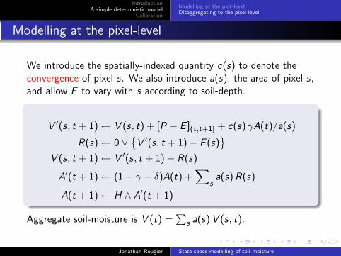
Modelling at the pixel-level
We introduce the spatially-indexed quantity c(s) to denote theconvergence of pixel s. We also introduce a(s), the area of pixel s,and allow F to vary with s according to soil-depth.
V ′(s, t + 1)← V (s, t) + [P − E ](t,t+1] + c(s) γA(t)/a(s)
R(s)← 0 ∨{V ′(s, t + 1)− F (s)
}V (s, t + 1)← V ′(s, t + 1)− R(s)
A′(t + 1)← (1− γ − δ)A(t) +∑
sa(s) R(s)
A(t + 1)← H ∧ A′(t + 1)
Aggregate soil-moisture is V (t) =∑
s a(s) V (s, t).
Jonathan Rougier State-space modelling of soil-moisture

IntroductionA simple deterministic model
Calibration
Modelling at the plot-levelDisaggregating to the pixel-level
Coweeta by pixels
Location of Coweeta measuring stations
Easting
Nor
thin
g
275400 275500 275600 275700 275800 275900 276000
3880
000
3880
200
3880
400
3880
600
3880
800
1
2
3
4
5
6
7
8
Jonathan Rougier State-space modelling of soil-moisture
IntroductionA simple deterministic model
Calibration
Modelling at the plot-levelDisaggregating to the pixel-level
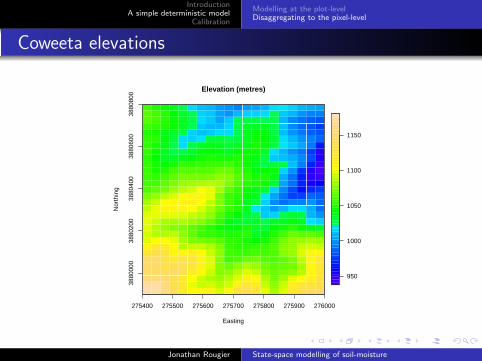
Coweeta elevations
275400 275500 275600 275700 275800 275900 276000
3880
000
3880
200
3880
400
3880
600
3880
800
Elevation (metres)
Easting
Nor
thin
g
950
1000
1050
1100
1150
Jonathan Rougier State-space modelling of soil-moisture

IntroductionA simple deterministic model
Calibration
Modelling at the plot-levelDisaggregating to the pixel-level
Coweeta convergence
275400 275500 275600 275700 275800 275900 276000
3880
000
3880
200
3880
400
3880
600
3880
800
Total Convergence Index
Easting
Nor
thin
g
60
80
100
120
140
33%
34%
6%
4%
5%
2%
4%
13%
Jonathan Rougier State-space modelling of soil-moisture

IntroductionA simple deterministic model
Calibration
Modelling at the plot-levelDisaggregating to the pixel-level
Coweeta soil-depth
275400 275500 275600 275700 275800 275900 276000
3880
000
3880
200
3880
400
3880
600
3880
800
Soil depth (cm)
Easting
Nor
thin
g
130
135
140
145
150
155
160
165
+5%
−3%
+0%
−3%
−1%
+7%
−1%
−4%
Jonathan Rougier State-space modelling of soil-moisture
IntroductionA simple deterministic model
Calibration
Modelling at the plot-levelDisaggregating to the pixel-level
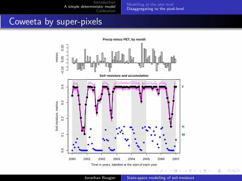
Coweeta by super-pixels
Precip minus PET, by month
met
res
−0.
100.
050.
20
2000 2001 2002 2003 2004 2005 2006 2007
0.0
0.1
0.2
0.3
0.4
Soil−moisture and accumulation
Time in years, labelled at the start of each year
Soi
l moi
stur
e, m
etre
s
W
H
F
●
●●●●
●
●
●
●
●
●
●
●
●●●●
●
●
●
●
●●●
●
●●●●
●
●
●
●
●
●
●●●●●●●
●●●●●●●●●●
●●●
●
●
●●
●●●●●●
●
●●●
●
●
●●●●●●
●
●
●
●
●
●
●●
●
●
●
●
●
●
●●●●●●●
●
●
●
●
●●●●●●●●
●●
●
●●
●
●●●●
●
●
●
●
●●
●
●
●●
●
●
●●
●
●
●
●
●●
●●
●
●
●
●●
●●
●
●
●
●
●
●
●
●
●●
●
●
●
●●●●●●
●
●
Jonathan Rougier State-space modelling of soil-moisture

IntroductionA simple deterministic model
Calibration
Modelling at the plot-levelDisaggregating to the pixel-level
Coweeta by pixels
Precip minus PET, by month
met
res
−0.
100.
050.
20
2000 2001 2002 2003 2004 2005 2006 2007
0.0
0.1
0.2
0.3
0.4
Soil−moisture and accumulation
Time in years, labelled at the start of each year
Soi
l moi
stur
e, m
etre
s
W
H
F
●
●●●●
●
●
●
●
●
●
●
●
●●●●
●
●
●
●
●●●
●
●●●●
●
●
●
●
●
●●●●●●●
●●●●●●
●●●●●●●●
●
●
●●
●●●●●●
●●●●
●
●
●●●●●●
●
●
●
●
●
●
●●
●
●
●
●
●
●
●●●●●●●
●
●
●
●
●●●●●●●●
●●
●
●●
●
●●●●
●
●
●
●
●●
●
●
●●
●
●
●●
●
●
●
●
●●
●●
●
●
●
●●
●●
●
●
●
●
●
●
●
●
●●
●
●
●
●●●●●●
●
●
Jonathan Rougier State-space modelling of soil-moisture

IntroductionA simple deterministic model
Calibration
Modelling at the plot-levelDisaggregating to the pixel-level
Findings so far . . .
Soil-moisture is an example of a fairly simple process subjectto complicated forcing.
Our simple model does a good job of showing how spatialheterogeneity causes variations in soil-moisture evolutionacross a plot, subject to common forcing. It is easy for us tointroduce further spatial factors, e.g., aspect and slope inevapotranspiration.
It’s a puzzle, though, why modelling at different resolutionsdoes not cause more variation in the aggregate quantitiesV (t) and A(t): possibly due to Coweeta being very wet?
If we want to widen the time-stepping, we need a carefultreatment of evapotranspiration and soil-moisture (the wiltingpoint, W , not discussed).
Jonathan Rougier State-space modelling of soil-moisture

IntroductionA simple deterministic model
Calibration
Looking ahead to calibration
We introduce a stochastic term accounting for modelimperfection, as part of the forcing:
V ′(s, t+1)← V (s, t)+[P−E ](t,t+1]+ω(s, t+1)+c(s) γA(t)/a(s)
Putting the uncertainty inside the model means that it doesnot contradict the physics. ω(s, t + 1) accounts mainly for(i) local differences in forcing; and (ii) local effects of run-off.
We can simulate our model forward. With some judiciouschoices we can calibrate using sequential Monte Carlomethods (aka particle filters).
Jonathan Rougier State-space modelling of soil-moisture
IntroductionA simple deterministic model
Calibration
Sequential calibration
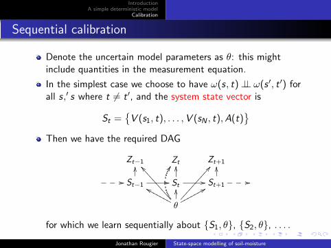
Denote the uncertain model parameters as θ: this mightinclude quantities in the measurement equation.
In the simplest case we choose to have ω(s, t)⊥⊥ ω(s ′, t ′) forall s,′ s where t 6= t ′, and the system state vector is
St ={V (s1, t), . . . ,V (sN , t),A(t)
}Then we have the required DAG
Zt−1 Zt Zt+1
//___ St−1//
OO
St//
OO
St+1
OO
//___
θ
ffNNNNNNN
^^<<<<<<<<<<OO
DD
88ppppppp
AA����������
for which we learn sequentially about {S1, θ}, {S2, θ}, . . . .
Jonathan Rougier State-space modelling of soil-moisture

IntroductionA simple deterministic model
Calibration
More generality
In the more general case where ω(s, t) 6⊥⊥ω(s ′, t ′) we wouldhave to include ω(t) in St , treating ω(t) as approximatelyMarkov.
To account for meter-specific measurement biases (likely to becommon and substantial in our case), we would have toinclude a vector of biases in θ.
For efficient calibration in these more general cases, it isimportant that we keep the number of pixels down (whichmeans we require fewer particles), and that we exploit largetime-steps where possible.
Jonathan Rougier State-space modelling of soil-moisture


