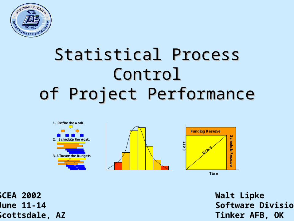
Statistical Process ControlStatistical Process Controlof Project Performanceof Project Performance
1. Define the work.
2. Schedule the work.
3. Allocate the Budgets100
50
80
20
50
10
20
Funding Reserve
Sch
edu
le Reserve
BCWS
Time
Co
st
Walt LipkeSoftware DivisionTinker AFB, OK
SCEA 2002June 11-14Scottsdale, AZ

2
ObjectiveObjective
To discuss the application ofTo discuss the application ofSPC Control Charts to the SPC Control Charts to the
EVM indicators,SPI and CPIEVM indicators,SPI and CPI
EVM
CPI
SPI
ControlCharts
SPC

3
OverviewOverview
• Introduction• SPC applied to Software Development?• Review EVM & SPC• SPC with EVM – Does What?• Problems / Cause• Solution Criteria• Proposed Solutions• Testing / Results• Summary
4
IntroductionIntroduction• Software Division
– SEI CMM Level 2 (1993) – First in Air Force– SEI CMM Level 4 (1996) – First in Federal Service– ISO 9001 / TickIT (1998)– IEEE / SEI Software Process Achievement Award (1999)
• EVM Facilitated the Achievements
5
Why SPC?Why SPC?
• SEI CMM Level 4 – Then & Now
• “Statistically Manage the Sub-process”
• CMM Evaluators “Show me the SPC Control Charts”
• Quality Control vs Performance Management

6
SPC ReviewSPC Review
• Several Methods Control Charts
• Control Charts Several Types
• Individuals and Moving Range
Average23 2 3
Process Behavior
AnomalousBehavior
AnomalousBehavior

7
Control ChartControl Chart
1 2 3 4 5 6 20 21 22 23 24 25
3σ
3σ
xObservedValues
Anomalous(“signal”)
Observations – in sequence

8
EVM ReviewEVM Review
Time
BCWS
ACWP
BCWP
$
Total Allocated Budget
Budget at Completion
Management Reserve
BCWS
BCWPSPI
ACWP
BCWPCPI
ProjectCompletion
Date
NegotiatedCompletion
Date
9
SPC with EVM – Does What?SPC with EVM – Does What?
• Performance Prediction– Probability of Success– EAC & ECD – range
• Project Planning– Historical Data– Risk MR Strategy
• Process Improvement– Plan Execution– Decreasing Variation

10
Planning/Performance/ImprovementPlanning/Performance/Improvement
Time
$$
3σ
3σ-
3σ
3σ-
Cost Distribution
Schedule Distribution
Performance Window (PW)
Negotiated Performance (> 50% PW)
Planned Performance (= 50% PW)
TotalAllocatedBudget
Budgetat
Completion
PlannedProject
Completion
NegotiatedProject
Completion
11
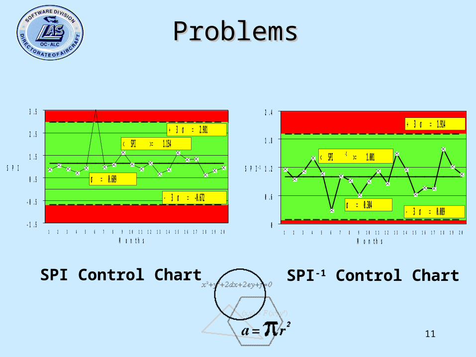
ProblemsProblems
SPI Control Chart SPI-1 Control Chart
- 1 . 5
- 0 . 5
0 . 5
1 . 5
2 . 5
3 . 5
1 2 3 4 5 6 7 8 9 1 0 1 1 1 2 1 3 1 4 1 5 1 6 1 7 1 8 1 9 2 0
2.9813 σ
-0.6723 σ
0.609σ
1.154SPI
S P I
M o n t h s
0
0 . 6
1 . 2
1 . 8
2 . 4
1 2 3 4 5 6 7 8 9 1 0 1 1 1 2 1 3 1 4 1 5 1 6 1 7 1 8 1 9 2 0
1.9143 σ
0.0893 σ 0.304σ
1.001SPI -1 S P I - 1
M o n t h s
12
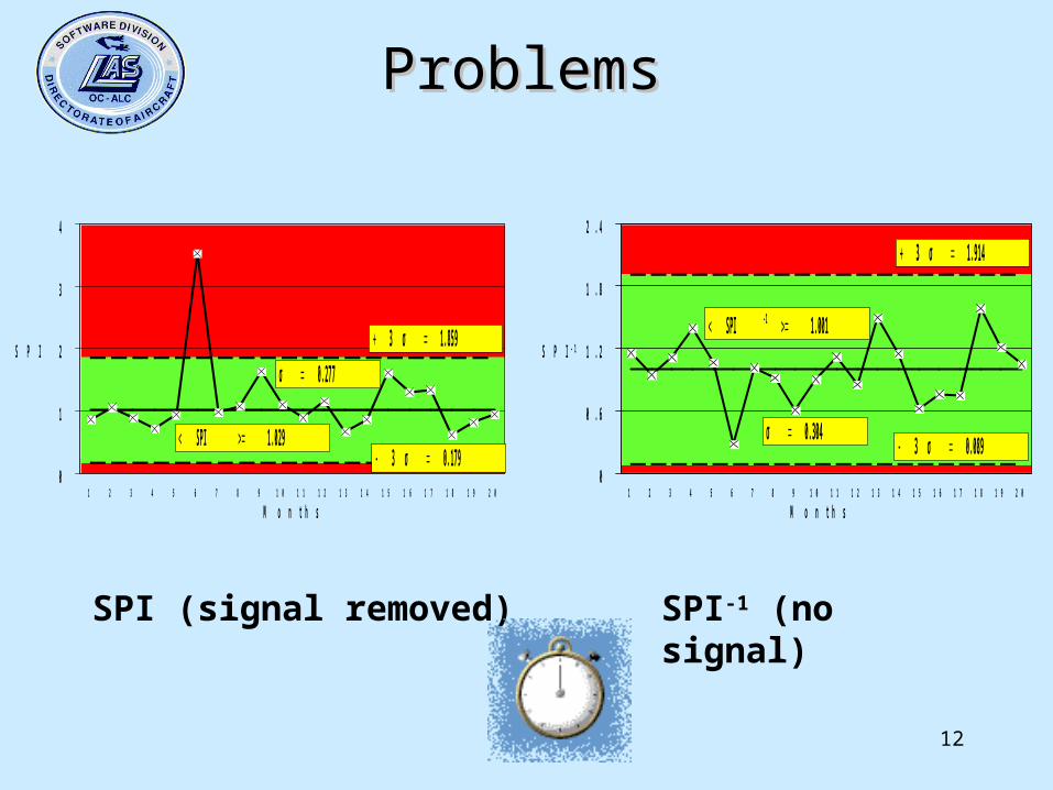
ProblemsProblems
SPI (signal removed) SPI-1 (no signal)
0
1
2
3
4
1 2 3 4 5 6 7 8 9 1 0 1 1 1 2 1 3 1 4 1 5 1 6 1 7 1 8 1 9 2 0
1.8593 σ
0.1793 σ
0.277σ
1.029SPI
S P I
M o n t h s
0
0 . 6
1 . 2
1 . 8
2 . 4
1 2 3 4 5 6 7 8 9 1 0 1 1 1 2 1 3 1 4 1 5 1 6 1 7 1 8 1 9 2 0
1.9143 σ
0.0893 σ 0.304σ
1.001SPI -1 S P I - 1
M o n t h s
13
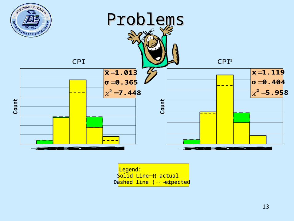
ProblemsProblems
Legend:Solid Line ( ) - actualDashed line ( ) - expected
Legend:Solid Line ( ) - actualDashed line ( ) - expected
7.448
0.365 σ
1.013 x
2
Count
CPI
3σ1.8σ 0.6σ 0.6σ1.8σ3σ
5.958
0.404 σ
1.119 x
2
Count
CPI-1
3σ1.8σ 0.6σ 0.6σ1.8σ3σ
14
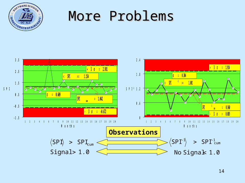
0
0 . 6
1 . 2
1 . 8
2 . 4
1 2 3 4 5 6 7 8 9 1 0 1 1 1 2 1 3 1 4 1 5 1 6 1 7 1 8 1 9 2 0
1.9143 σ
0.0893 σ
0.304σ 1.001SPI -1
S P I - 1
M o n t h s
0.960SPI cum-1
- 1 . 5
- 0 . 5
0 . 5
1 . 5
2 . 5
3 . 5
1 2 3 4 5 6 7 8 9 1 0 1 1 1 2 1 3 1 4 1 5 1 6 1 7 1 8 1 9 2 0
2.9813 σ
-0.6723 σ
0.609σ
1.154SPI
S P I
M o n t h s
1.042SPI cum
More ProblemsMore Problems
1.0 Signal
SPI SPI cum
1.0 Signal No
SPI SPI cum-1-1
Observations

15
Problem ExampleProblem Example
-2
-1
0
1
2
3
4
5
3σ
3σ
SPI
aSPI
bSPI
-2
-1
0
1
2
3
4
5
3σ
3σ
-1SPI
a-1SPI
b-1SPI
SP
I
SP
I-1

16
Problem SummaryProblem Summary
• <PI> > PIcum & <PI-1> > PI-1cum
• <PI>-1 <PI-1> • Signals (nearly always) > 1.0• PI signals PI-1 signals• PI sigma PI-1 sigma• Histograms Normal Distribution
• Without Resolution SPC Application
17
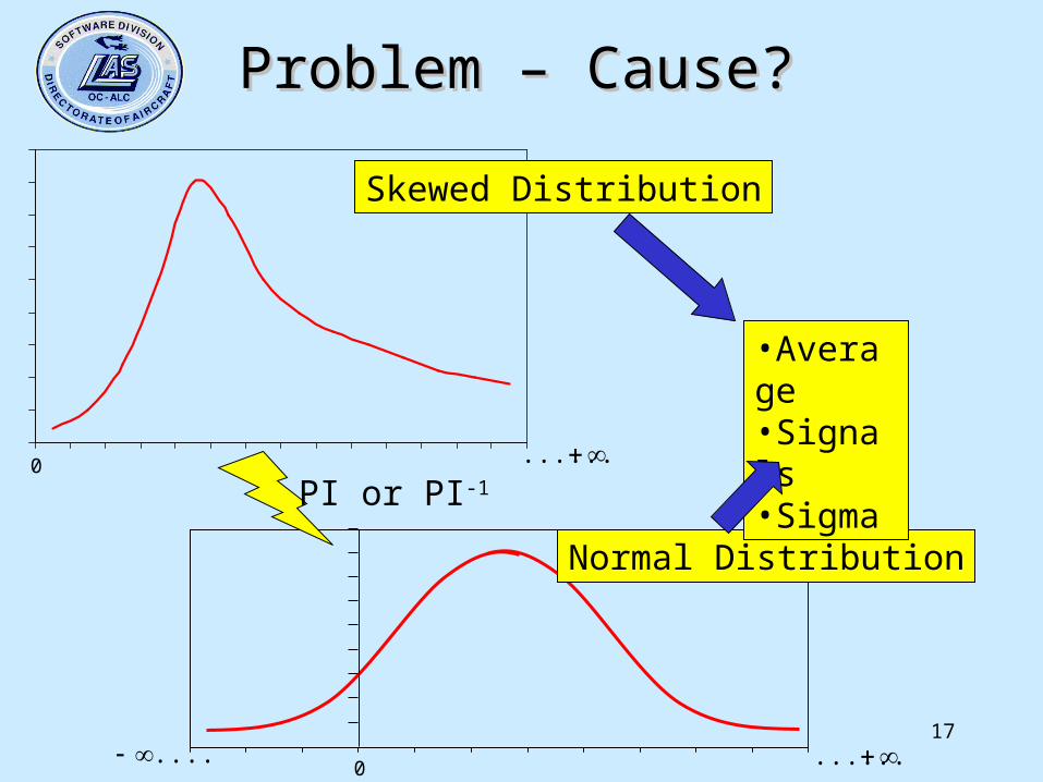
Problem – Cause?Problem – Cause?
......
...............
0
0
PI or PI-1
Skewed Distribution
Normal Distribution
•Average•Signals•Sigma
18
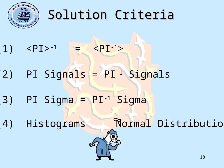
Solution CriteriaSolution Criteria
(1) <PI>-1 = <PI-1>
(2) PI Signals = PI-1 Signals
(3) PI Sigma = PI-1 Sigma
(4) Histograms Normal Distribution
19
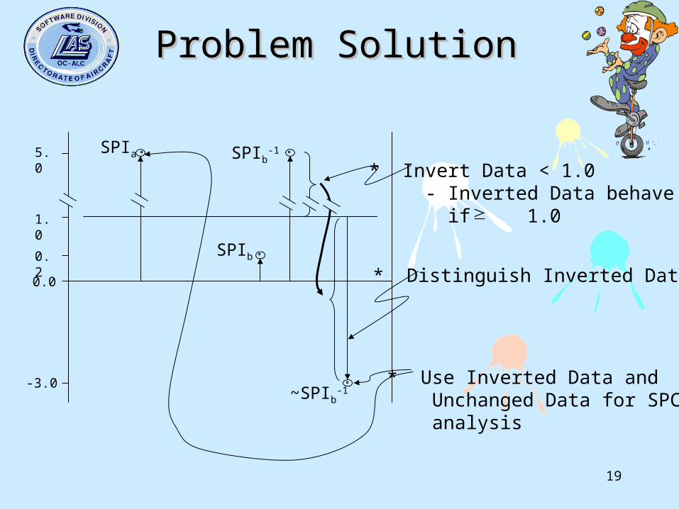
Problem SolutionProblem Solution
0.0
0.2
1.0
5.0
-3.0
* Invert Data < 1.0 - Inverted Data behave as if 1.0
* Distinguish Inverted Data
* Use Inverted Data and Unchanged Data for SPC analysis
SPIa SPIb-1
SPIb
~SPIb-1

20
Data Transform RulesData Transform RulesData Transform RulesData Transform Rules
• If PI 1.0, then ~PI = PI
• If PI < 1.0, then ~PI = 2 - PI-1
• If ~PI 1.0, then PIu = <~PI>
• If ~PI < 1.0, then PIu = (2- ~PI)-1
Perform SPC analysis with Transformed Data

21
Problem Solution -ExampleProblem Solution -Example
-2
-1
0
1
2
3
4
5
2.6SPI
aSPI
bSPI
-3
-2
-1
0
1
2
3
4
5
1.0SPIu
bSPI~
aSPI~
SP
I
~S
PI

22
0
0 . 5
1
1 . 5
2
2 . 5
3
3 . 5
4
1 2 3 4 5 6 7 8 9 1 0 1 1 1 2 1 3 1 4 1 5 1 6 1 7 1 8 1 9 2 0
1.9783 σ
0.0163 σ
0.327σ
0.997SPI~u
~ S P I
M o n t h s
- 2
- 1 . 5
- 1
- 0 . 5
0
0 . 5
1
1 . 5
2
2 . 5
1 2 3 4 5 6 7 8 9 1 0 1 1 1 2 1 3 1 4 1 5 1 6 1 7 1 8 1 9 2 0
1.9843 σ
0.0223 σ
0.327σ
1.003SPI~u
-1
~ S P I - 1
M o n t h s
Proposed Solution EvaluationProposed Solution Evaluation
• Demonstrates meeting criteria 1, 2, and 3• Mathematically meets criteria 1, 2, and 3• Proof enough?

23
Co
un
t
5.9582
0.214)P( 2 4.6432
Co
un
t
0.341)P( 2
Data Transform –Data Transform –Histogram TestHistogram Test
3σ1.8σ 0.6σ 0.6σ1.8σ3σ3σ1.8σ 0.6σ 0.6σ1.8σ3σ3σ1.8σ 0.6σ 0.6σ1.8σ3σ3σ1.8σ 0.6σ 0.6σ1.8σ3σ
CPI-1 Histogram ~CPI-1 Histogram
areas. histogram the of one is i where,
count /expected)count expectedcount (observed ii
2ii
2
24
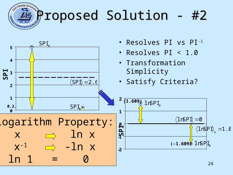
Proposed Solution - #2Proposed Solution - #2
0
1
2
3
4
5
2.6SPI
aSPI
bSPI
-2
-1
0
1
2
1.0SPI lnu
bSPI ln
aSPI ln
SP
I
ln S
PI
0.2
0SPI ln
(1.609)
(-1.609)
• Resolves PI vs PI-1
• Resolves PI < 1.0• Transformation Simplicity• Satisfy Criteria?
Logarithm Property:x ln xx-1 -ln x
ln 1 = 0
25
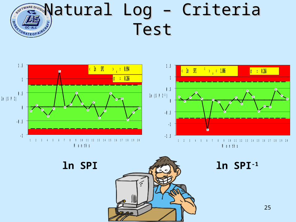
- 1
- 0 . 5
0
0 . 5
1
1 . 5
1 2 3 4 5 6 7 8 9 1 0 1 1 1 2 1 3 1 4 1 5 1 6 1 7 1 8 1 9 2 0
0.266σ 0.994SPI ln u
l n ( S P I )
M o n t h s
- 1 . 5
- 1
- 0 . 5
0
0 . 5
1
1 . 5
1 2 3 4 5 6 7 8 9 1 0 1 1 1 2 1 3 1 4 1 5 1 6 1 7 1 8 1 9 2 0
0.266σ 1.006SPI ln u-1
l n ( S P I - 1 )
M o n t h s
Natural Log – Criteria TestNatural Log – Criteria Test
ln SPI ln SPI-1
26
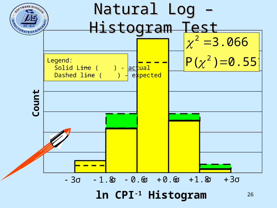
Natural Log – Histogram TestNatural Log – Histogram Test
0.551)P(
3.0662
2
Co
un
t
Legend: Solid Line ( ) - actual Dashed line ( ) - expected
3σ 1.8σ 0.6σ 0.6σ 1.8σ 3σ
ln CPI-1 Histogram

27
Testing SummaryTesting Summary
Test Raw Transformation Logarithm
1. PI-1 = PI-1 No Yes Yes
2. PI Signals = PI-1 Signals No Yes Yes
3.PI Sigma = PI-1 Sigma
No Yes Yes
4. Histograms ~ Normal DistributionVery
UnlikelyUnlikely Likely

28
Sensitivity AnalysisSensitivity Analysis
0
0.02
0.04
0.06
0.08
0.1
0.12
0 0.1 0.2 0.3 0.4 0.5 0.6 0.7
SPIs
(0.284,0.025)
SPI(0.625,0.112)
SPIsu
(0.327,0.007)
SPIu
(0.651,0.082)
lnSPIsu
(0.266,0.01)
lnSPIu
(0.384,0.018)
P
I-
PI c
um
Note: 1. Subscript s indicates the signal is removed from the calculations.2. Subscript u indicates the average value is untransformed from
the average value determined from the SPC analysis

29
SummarySummary
• SPC application to Software Development
• SPC applied to CPI & SPI– Project Execution– Project Planning– Process Improvement
• Problems– Data Representation– SPC Results

30
SummarySummary
• Solutions– Data Transform– Natural logarithm
• Criteria– Results independent from data representation– Results derived from Normal Distribution
• Testing/Results– Data Transform – Good– Natural Logarithm - Better
31
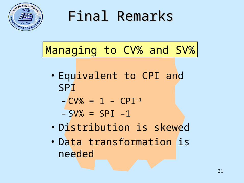
Final RemarksFinal Remarks
• Equivalent to CPI and SPI– CV% = 1 – CPI-1
– SV% = SPI –1
• Distribution is skewed
• Data transformation is needed
Managing to CV% and SV%
32
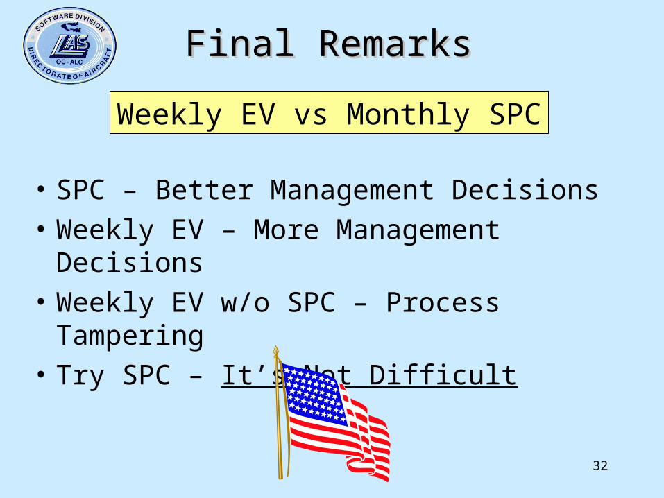
Final RemarksFinal Remarks
• SPC – Better Management Decisions
• Weekly EV – More Management Decisions
• Weekly EV w/o SPC – Process Tampering
• Try SPC – It’s Not Difficult
Weekly EV vs Monthly SPC


