
Stochastic Modeling in Systems Biology and Biophysics
Subhadip Raychaudhuri
Indraprastha Institute of Information Technology Delhi(IIITD)
Fundamentals of Systems BiologyUniversity of Delhi Dec 24 (2014)

Variability in single cell gene expressions elucidates genetic architecture within a tumor
Single cell gene expressions reveal genetic diversity in leukemia
Nature 469:356-361 (2011)Nature 469:362-366 (2011)
Fluorescence in situ hybridization with ERBB2 probes (red) and centromere of chromosome 17 (red)
PLoS One 9:e1079582 copies
> 10 copies

Apoptosis resistance of cancer cells
• Cancer cells are characterized by their remarkable resistance to apoptotic cell death (frequently by expressing apoptotic inhibitors in abundance)
variability in time-to-death
(Apoptosis 15:1223-1233 (2010)Experiments by J. Skommer and T.Brittain

Selective killing of cancer cells under Bcl2 inhibition
Cancer cells under Bcl2 inhibition
Cancer cells without Bcl2 inhibition(Bcl2 / Bax > 1)
Journal of Healthcare Eng. 4:47-66 (2013)S. Raychaudhuri and S.C. Das

Elowitz et al, Science, 297, 1183 (2002)
Noisy gene expression
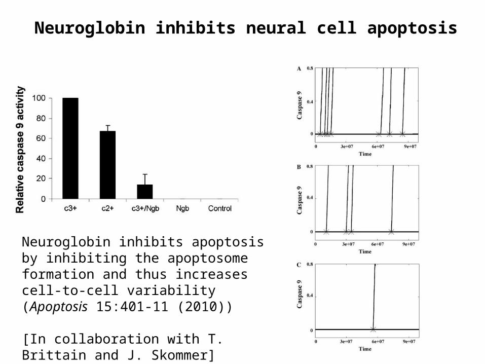
Neuroglobin inhibits neural cell apoptosis
Neuroglobin inhibits apoptosis by inhibiting the apoptosome formation and thus increases cell-to-cell variability (Apoptosis 15:401-11 (2010))
[In collaboration with T. Brittain and J. Skommer]

What is common in all these?
Cell-to-cell stochastic variability (stochastic fluctuation)

Stochastic fluctuations / Stochastic variability / Noise
Some more examples ……..

Analysis of single cell gene expressions can provide insight into cancer and degenerative disorders
Single cell gene expressions provide insight into genetic diversity in a tumor cell population
Single cell study seems to be important in elucidating cancer
stem cells and apoptosis resistance
Single cell gene expressions could elucidate molecular pathogenesis of various neurological diseases
Nature 469:356-361 (2011)Nature 469:362-366 (2011)NeuroRx: 3:302-318 (2006)

Selective killing of cancer cells by targeting the apoptotic pathway
Variability in cell-to-cell stochastic fluctuation in apoptotic activation between cancer and healthy cells can be utilized in selective targeting
In certain cancers, a stochastic to deterministic transition in apoptotic activation might be possible to achieve (such as type 2 type 1 transition)
Healthy cells should mostly remain protected by large cell-to-cell variability in apoptotic activation
Increasing cell-to-cell variability in apoptosis can be a strategy to treat degenerative disorders
Caspase 6 inhibition may lead to type 1 type 2 transition in a large number of neural cells that are undergoing degeneration
Increasing the Bcl2/Bax ratio (to > 1) or lowering the probability of apoptosome formation can also be effective in certain cases
Systems and Synthetic Biology8:83-97 (2014)
PLoS One 5:e13437 (2010)
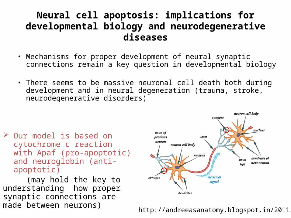
Neural cell apoptosis: implications for developmental biology and neurodegenerative diseases
• Mechanisms for proper development of neural synaptic connections remain a key question in developmental biology
• There seems to be massive neuronal cell death both during development and in neural degeneration (trauma, stroke, neurodegenerative disorders)
http://andreeasanatomy.blogspot.in/2011/04/
Our model is based on cytochrome c reaction with Apaf (pro-apoptotic) and neuroglobin (anti-apoptotic)
(may hold the key to understanding how proper synaptic
connections are made between neurons)

Mechanisms for single cell origin of cancer
Cancer cells seem to originate from a single cell (one single cell out of many healthy cells start clonal expansion of a tumor)
Mutation in a single oncogene (such as Bcl2) may lead to increased cell-to-cell variability (resulting in slow activation) in apoptotic activation
Biology of Cancer, by Weinberg

Mechanisms for single cell origin of neural stem cells
Neural stem cells seem to originate from a single cell (one single cell out of several similar cells)
A simple feed-back activation based model of Notch-Delta signaling can provide insight into single cell mechanisms for origin of neural stem cells
Principles of DevelopmentWolpert & Tickle
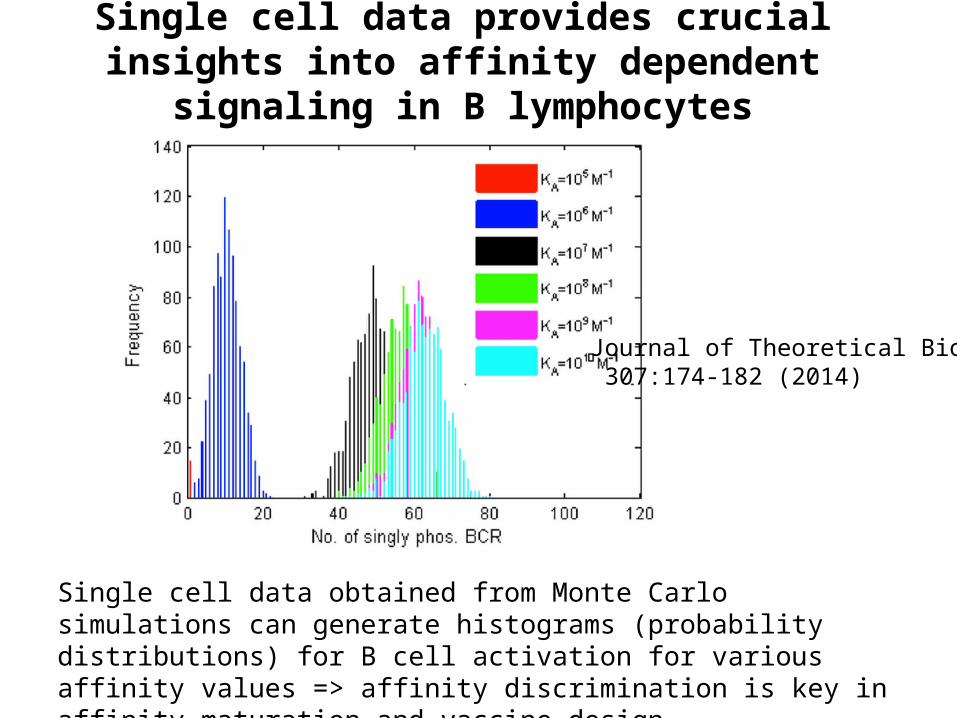
Single cell data provides crucial insights into affinity dependent signaling in B lymphocytes
Single cell data obtained from Monte Carlo simulations can generate histograms (probability distributions) for B cell activation for various affinity values => affinity discrimination is key in affinity maturation and vaccine design
Journal of Theoretical Biology 307:174-182 (2014)

Modeling of stochastic processes:some historical examples
Random walk motion known as Brownian motion (diffusion equation approach by Einstein and stochastic equation of Langevin)
Fluctuations in stock markets (diffusion equation and stochastic equation)
Fluctuations in birth-death processes (such as in population biology)(modeled using Master equations)
Noise in electronic systems (Master equations)
Stochastic Methods by C. Gardiner
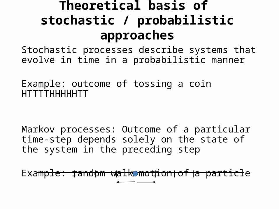
Theoretical basis of stochastic / probabilistic approaches
Stochastic processes describe systems that evolve in time in a probabilistic manner
Example: outcome of tossing a coin HTTTTHHHHHTT
Markov processes: Outcome of a particular time-step depends solely on the state of the system in the preceding step
Example: random walk motion of a particle
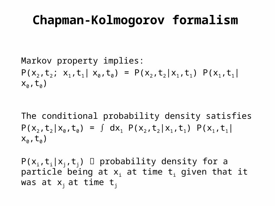
Chapman-Kolmogorov formalism
Markov property implies:P(x2,t2; x1,t1| x0,t0) = P(x2,t2|x1,t1) P(x1,t1|x0,t0)
The conditional probability density satisfies P(x2,t2|x0,t0) = dx1 P(x2,t2|x1,t1) P(x1,t1|x0,t0)
P(xi,ti|xj,tj) probability density for a particle being at xi at time ti given that it was at xj at time tj

Master equation formalism
Pi(t) probability that the system is in state i at time t
Wij(t) transition probability from state j i
Master equation for a simple random walk

Master equation formalism
Master equation for a simple random walk
Continuum limit of the RW Master equation
Known as Fokker-Planck equation(obtained by Taylor expanding P(x l,t))
Can be obtained as (i) Differential form of Chapman-Kolmogorov equation(ii) From the corresponding stochastic equation (Langevin equation)

In Silico approach
• Monte Carlo (stochastic) simulations solving master equations on a computer stochastic simulations can capture dynamics of
biological processes
• Stochastic equations may also provide insight into certain cases (such as in the underlying design principles of a robust functional response)

Stochastic simulation approach
• Gillespie’s stochastic simulation algorithm (SSA)
• Kinetic Monte Carlo simulations Both involve solving master equations on a
computer (in silico)
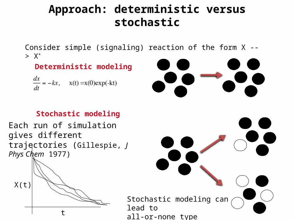
Approach: deterministic versus stochastic
Consider simple (signaling) reaction of the form X --> X*
Deterministic modeling
Stochastic modeling
Each run of simulation gives different trajectories (Gillespie, J Phys Chem 1977)
X(t)
t
Stochastic modeling can lead toall-or-none type behavior

Approach: deterministic versus stochastic
Consider simple (signaling) reaction of the form X --> X*
Deterministic modeling
Above ODE is obtained in the following manner:
When x(t) or k is very small ODE limit is no longer valid=> Instead, kxΔt can be considered as the probability of reaction

Gillespie’s Stochastic simulation approach
Start with Master equation that describes the time-evolution equation for the function P(X1, X2, …XN, t)
P(X1, X2, …XN, t+dt) = P(X1, X2, …XN;t)[1 - aμ dt] + Bμ dt
=> /t P(X1, X2, …XN, t) = [ Bμ - aμ P(X1, X2, …XN, t) ]
Probability that the next reaction will occur after time τP0(τ) = exp (- aν τ)
Probability that the next reaction will be the μth reaction
P(μ) = aν < r a0 ≤ aν a0 = aν
μ-1 μ M

Kinetic Monte Carlo simulation approach
Start with Master equation that describes the time-evolution equation for the function P(X1, X2, …XN, t)
P(X1, X2, …XN, t+dt) = P(X1, X2, …XN;t)[1 - aμ dt] + Bμ dt
=> /t P(X1, X2, …XN, t) = [ Bμ - aμ P(X1, X2, …XN, t) ]
Define a set of probability constants aμ Δt (from state X1, X2, …XN, t)
At each Monte Carlo step carry out moves with r < aμ Δt

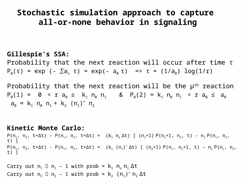
Stochastic simulation approach to capture all-or-none behavior in signaling
Start with Master equation for the function P(X1, X2, …XN, t)
/t P(n1, n2, t) = k no [ (n1+1) P(n1+1, n2, t) - n1 P(n1, n2, t) ] + k (n1)*
[ (n2+1) P(n1, n2+1, t) – n2 P(n1, n2, t) ]
Stochastic simulation approach to capture all-or-none behavior in signaling
Gillespie’s SSA:Probability that the next reaction will occur after time τP0(τ) = exp (- aν τ) = exp(- a0 τ) => τ = (1/a0) log(1/r)
Probability that the next reaction will be the μth reactionP0(1) = 0 < r a0 ≤ k1 n0 n1 & P0(2) = k1 n0 n1 < r a0 ≤ a0 a0 = k1 n0 n1 + k2 (n1)* n2
Kinetic Monte Carlo:P(n1, n2, t+Δt) - P(n1, n2, t+Δt) = (k1 no Δt) [ (n1+1) P(n1+1, n2, t) - n1 P(n1, n2, t) ]P(n1, n2, t+Δt) - P(n1, n2, t+Δt) = (k2 (n1)*
Δt) [ (n2+1) P(n1, n2+1, t) – n2 P(n1, n2, t) ]
Carry out n1 n1 – 1 with prob = k1 no n1 ΔtCarry out n2 n2 – 1 with prob = k2 (n1)*
n2 Δt

Stochastic simulation approach to capture all-or-none behavior in signaling
Kinetic Monte Carlo simulation
Time MC step = 0.1 sec
Gillespie’s SSA
Time (sec)
Activ
ation
of x
2

Implementation of kinetic Monte Carlo (MC)
Simulation is carried out on a cubic lattice Only one molecule per node
Signaling molecules can diffuse in 2D (surface bound) or in 3D (intracellular) with specified probability of diffusion Pdiff
Signaling molecules undergo reactions with specified probabilities Pon, Poff, Pcat.
One simulation run (single cell) takes between ~ minutes to ~ days (using a reduced system size for computationally intensive simulations)
Lattice picture: http://www.mikeblaber.org/oldwine/chm1045/notes/Forces/Solids/lattice.gif
Schematics of the 3D simulation lattice

Kinetic Monte Carlo algorithm
• Pick any molecule at random
• Two different types of move: Diffusion or reaction (determined by unbiased coin toss)
• Diffusion move: Equal probability of moving to any unoccupied neighboring sites (pdiff)
Is selected node unoccupied? pdiff
Kinetic Monte Carlo algorithm
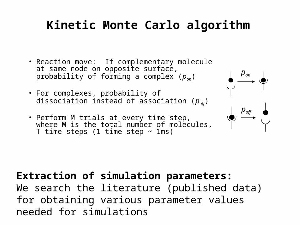
• Reaction move: If complementary molecule at same node on opposite surface, probability of forming a complex (pon)
• For complexes, probability of dissociation
instead of association (poff)
• Perform M trials at every time step, where M is the total number of molecules, T time steps (1 time step ~ 1ms)
pon
poff
Extraction of simulation parameters: We search the literature (published data) for obtaining various parameter values needed for simulations
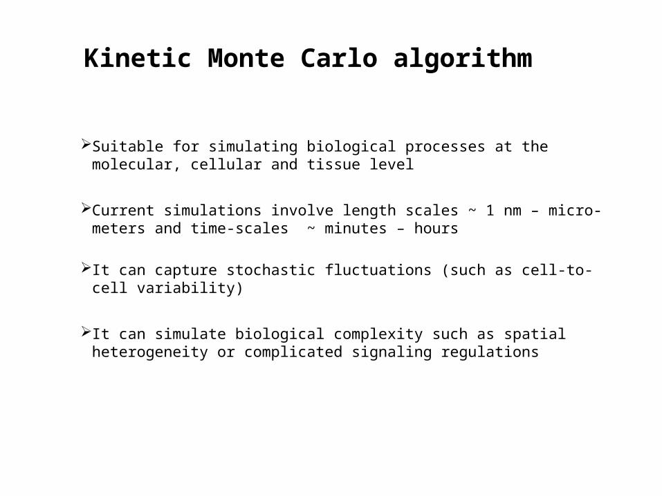
Kinetic Monte Carlo algorithm
Suitable for simulating biological processes at the molecular, cellular and tissue level
Current simulations involve length scales ~ 1 nm – micro-meters and time-scales ~ minutes – hours
It can capture stochastic fluctuations (such as cell-to-cell variability)
It can simulate biological complexity such as spatial heterogeneity or complicated signaling regulations

Hybrid approaches in kinetic Monte Carlo
Suitable for simulating very complex biological processes (Often such simulations span multiple length and time scales)
Hybrid simulation to capture the dynamics of receptor-lipid raft formation involve systems level approach combining:• Diffusion of membrane molecules (receptors and lipids) based on
energetics (thermodynamic free energy and detail balance)• Probabilistic rate constant based kinetic MC for membrane proximal and
intracellular signaling • Membrane shape fluctuations (governed by membrane mechanical
properties surface tension and bending rigidity that will depend on lipid composition of the membrane)

Modeling of stochastic variability in biology: type 1/type 2 choice in apoptotic cell death
and selective killing of cancer cells
Single cell approach is essential in elucidating
the type 1/ type 2 choice in apoptotic cell death (a key problem in the biology of apoptosis)
the mechanisms for selective killing of cancer cells (that would protect healthy cells)

Apoptotic death signaling pathway
Elucidating the systems level mechanisms may answer many important basic questions in the biology of apoptosis
Extrinsic(Type 1)
Intrinsic(Type 2)
Taken from: EMBO reports5:674-678 (2004)

Single cell biology of apoptosis activation in silico
Time 1
Time 2
S. Raychaudhuri, E. Willgohs, T-N. Nguyen, E. Khan, T. Goldkorn
Biophysical Journal 2008
Time (~ minutes) Time (~ hours)
activecaspase-3
Type 1 Type 2
Time (~ minutes) Time (~ hours)
1 1
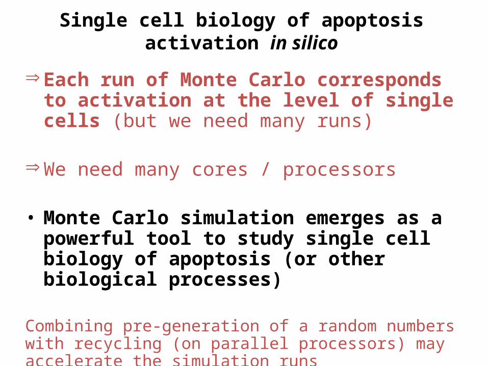
Single cell biology of apoptosis activation in silico
Each run of Monte Carlo corresponds to activation at the level of single cells (but we need many runs)
We need many cores / processors
• Monte Carlo simulation emerges as a powerful tool to study single cell biology of apoptosis (or other biological processes)
Combining pre-generation of a random numbers with recycling (on parallel processors) may accelerate the simulation runs => pre-generated sequence of accept/reject moves

Data analysis for single cell biology of apoptosis activation
• Monte Carlo simulation emerge as a powerful tool to study single cell biology of apoptosis (or other biological processes)
• New challenges involved in data analysis (such as estimating time-to-death)
• Probability distribution based approaches turn out to be insightful
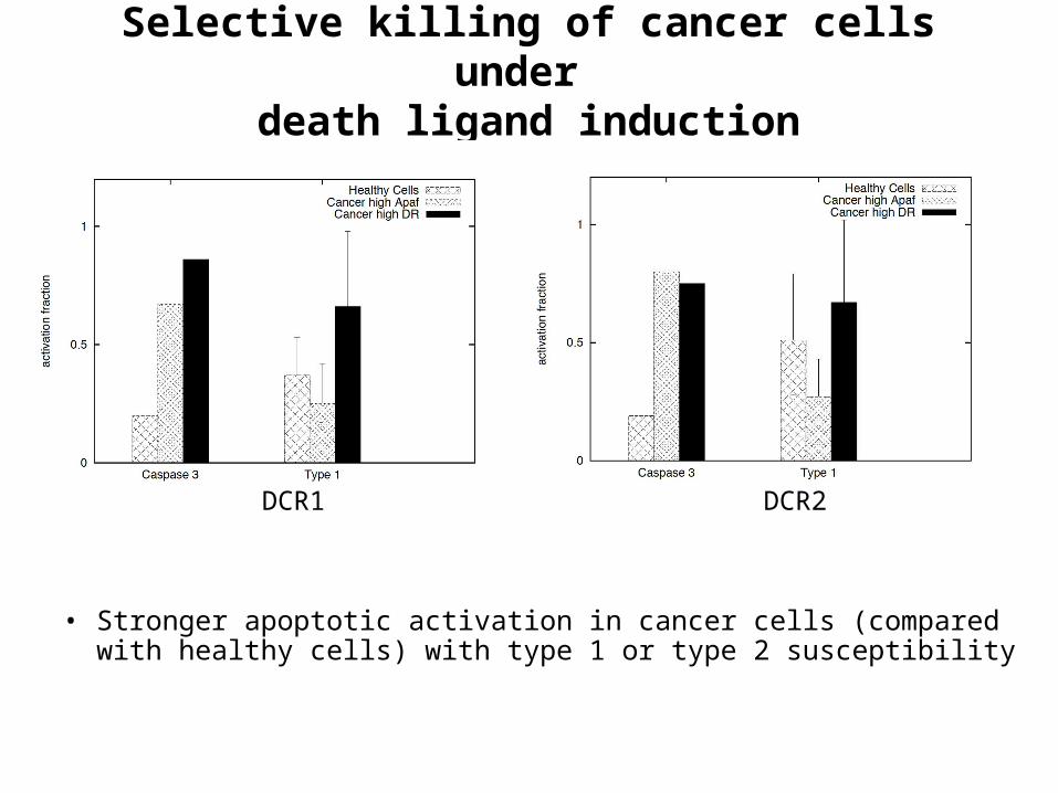
Selective killing of cancer cells under death ligand induction
• Stronger apoptotic activation in cancer cells (compared with healthy cells) with type 1 or type 2 susceptibility
DCR1 DCR2

Selective killing of cancer cells under death ligand induction
• Significant differences in cell-to-cell variability (in apoptosis activation) between healthy and cancer cells
Decoy receptor 1 (DCR1) = 20, DL = 5

Selective killing of cancer cells under death ligand induction
• Significant differences in cell-to-cell variability (in apoptosis activation) between healthy and cancer cells
Decoy receptor 2 (DCR2) = 20, DL = 5

Cell-to-cell variability in biological Processes
Cell-to-cell variability in biological dynamics may arise due to
• Inherent cell-to-cell differences in the genomic and proteomic state
• Inherent fluctuations in signaling reactions (arise when low number of molecules are present, low number of molecules emerge due to inhibition or low probability of reaction is involved)
• Often these two effects are synergistic leading to large cell-to-cell stochastic variability in response
(may result in distinct functional outcomes and signaling phenotypes)


