
Syracuse University Syracuse University
SURFACE SURFACE
Theses - ALL
5-2015
STRESS-STRAIN BEHAVIOR BY IMAGE ANALYSIS, MIX DENSITY STRESS-STRAIN BEHAVIOR BY IMAGE ANALYSIS, MIX DENSITY
AND PRE-STRAIN EFFECTS OF EPS GEOFOAM AND PRE-STRAIN EFFECTS OF EPS GEOFOAM
Chen Liu Syracuse University
Follow this and additional works at: https://surface.syr.edu/thesis
Part of the Civil and Environmental Engineering Commons
Recommended Citation Recommended Citation Liu, Chen, "STRESS-STRAIN BEHAVIOR BY IMAGE ANALYSIS, MIX DENSITY AND PRE-STRAIN EFFECTS OF EPS GEOFOAM" (2015). Theses - ALL. 103. https://surface.syr.edu/thesis/103
This Thesis is brought to you for free and open access by SURFACE. It has been accepted for inclusion in Theses - ALL by an authorized administrator of SURFACE. For more information, please contact [email protected].
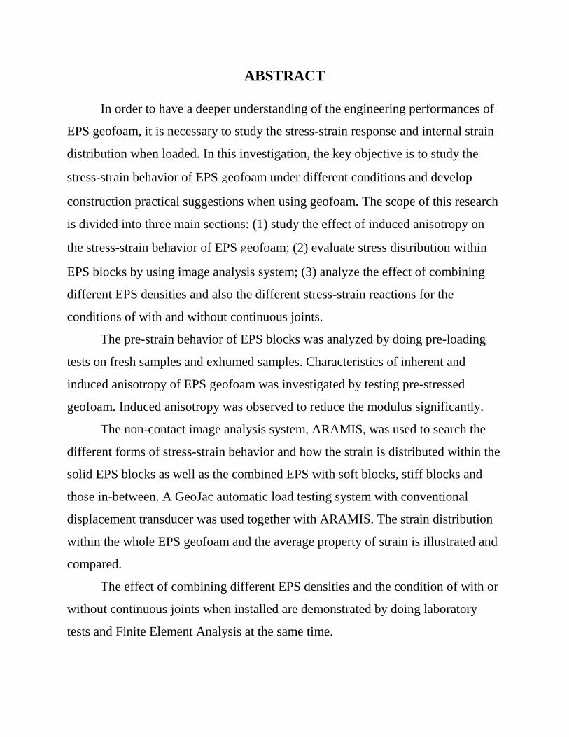
ABSTRACT
In order to have a deeper understanding of the engineering performances of
EPS geofoam, it is necessary to study the stress-strain response and internal strain
distribution when loaded. In this investigation, the key objective is to study the
stress-strain behavior of EPS geofoam under different conditions and develop
construction practical suggestions when using geofoam. The scope of this research
is divided into three main sections: (1) study the effect of induced anisotropy on
the stress-strain behavior of EPS geofoam; (2) evaluate stress distribution within
EPS blocks by using image analysis system; (3) analyze the effect of combining
different EPS densities and also the different stress-strain reactions for the
conditions of with and without continuous joints.
The pre-strain behavior of EPS blocks was analyzed by doing pre-loading
tests on fresh samples and exhumed samples. Characteristics of inherent and
induced anisotropy of EPS geofoam was investigated by testing pre-stressed
geofoam. Induced anisotropy was observed to reduce the modulus significantly.
The non-contact image analysis system, ARAMIS, was used to search the
different forms of stress-strain behavior and how the strain is distributed within the
solid EPS blocks as well as the combined EPS with soft blocks, stiff blocks and
those in-between. A GeoJac automatic load testing system with conventional
displacement transducer was used together with ARAMIS. The strain distribution
within the whole EPS geofoam and the average property of strain is illustrated and
compared.
The effect of combining different EPS densities and the condition of with or
without continuous joints when installed are demonstrated by doing laboratory
tests and Finite Element Analysis at the same time.
STRESS-STRAIN BEHAVIOR BY IMAGE ANALYSIS, MIX DENSITY AND PRE-STRAIN EFFECTS OF EPS GEOFOAM
By
Chen Liu B.S., China University of Geosciences, Beijing, China, 2012
Dissertation submitted in partial fulfillment of the
requirements for the degree of
Master of Science in Civil Engineering
Syracuse University, Syracuse, New York
May 2015

Copy right © Chen Liu, 2015
All Rights Reserved

Acknowledgements
I would like to express my sincere appreciation to my thesis advisor,
Professor Dawit Negussey for the continuous encouragement and guidance of my
master study and research, for his patience, motivation, enthusiasm, and immense
knowledge. His support helped me in all the time of research and writing of this
thesis.
In addition, special thanks to Dr. S.K. Bhatia, Dr. Lui and Dr. H. Ataei for
their valuable suggestions, insightful comments, and hard questions. I am grateful
to all the people who contributed their efforts and time toward the completion of
this research.
My graduate assistantship provided by the Department of Civil and
Environmental Engineering throughout my course of study at Syracuse University
is also appreciated. Thanks to all my friends and fellow graduate students for
making my more than two years of graduate school more pleasant and meaningful.
Last but not the least, I would like to thank my family: my parents Dewei
Liu and Guobi Chen, for giving birth to me at the first place and supporting me
financially and spiritually throughout my life.
iv

Table of Contents
Acknowledgements………………………………………………………….…….iv
Table of Contents ....................................................................................................... v
Figures and Tables ................................................................................................. viii
CHAPTER 1 .............................................................................................................. 1
INTRODUCTION ..................................................................................................... 1
1.1 The History and Development of EPS Geofoam ............................................. 1
1.2 Geofoam - EPS in Geotechnical Applications ................................................. 1
1.3 Area of Study and Purpose of Research .......................................................... 3
CHAPTER 2 .............................................................................................................. 5
GEOFOAM UNCONFINED COMPRESSION TESTS AND PROPERTIES ........ 5
2.1 Unconfined/Uniaxial Compression Test .......................................................... 5
2.1.1 Test Specifications .................................................................................... 6
2.1.2 Test Results ............................................................................................... 8
2.2 EPS Properties................................................................................................10
2.2.1 Young’s Modulus ....................................................................................11
2.2.2 Sample Size and Density ........................................................................12
2.2.3 Compressive Strength and Insulation Property ......................................27
2.2.4 Creep Behavior .......................................................................................28
CHAPTER 3 ............................................................................................................31
PRE-STRAIN INDUCED ANISOTROPY OF EPS GEOFOAM ..........................31
3.1 Background ....................................................................................................31
v
3.2 Test Procedures ..............................................................................................34
3.2.1 Tests on Exhumed Samples from Field ..................................................34
3.2.2 Lab Tests on Different Pre-strain Conditions .........................................38
3.3 Conclusions ....................................................................................................53
CHAPTER 4 ............................................................................................................54
STRESS DISTRIBUTION WITHIN EPS BLOCKS BY USING IMAGE
ANALYSIS ..............................................................................................................54
4.1 Background ....................................................................................................54
4.2 ARAMIS System ...........................................................................................55
4.3 Test Procedure................................................................................................56
4.3.1 ARAMIS Setup .......................................................................................58
4.3.2 EPS Samples ...........................................................................................62
4.3.3 Principles of Operation ...........................................................................64
4.3.4 Test Results .............................................................................................69
4.4 Conclusions ....................................................................................................81
CHAPTER 5 ............................................................................................................83
EFFECTS OF COMBINING DIFFERENT DENSITIES .......................................83
AND LOCATION OF THE EPS BLOCKS ............................................................83
5.1 Background ....................................................................................................83
5.2 Lab Test Setup ...............................................................................................83
5.3 Lab Test Process ............................................................................................84
5.4 Test Results ....................................................................................................87
vi

5.5 FLAC 7.0 Modeling Results ..........................................................................95
5.6 Conclusions ..................................................................................................107
CHAPTER 6 ..........................................................................................................109
CONCLUSIONS AND RECOMMENDATIONS ................................................109
Appendix: Rotation Matrices .................................................................................112
1. Derivation of 2D Rotation Matrix .................................................................112
2. Derivation of 3D Elementary Rotation Matrices ...........................................114
References ..............................................................................................................119
vii
Figures and Tables
List of Figures:
Figure 2.1. GeoJac Load Frame Setup ............................................................... 7
Figure 2.2. GeoJac System Hardware Setup ...................................................... 8
Figure 2.3. Typical Stress-Strain Behavior for EPS Specimen ......................... 9
Figure 2.4. Initial Tangent Moduli of EPS Geofoam from Previous
Investigations ...........................................................................................12
Figure 2.5. EPS Uniaxial Compression Stress-Strain Curves (after Negussey
and Elragi, 2000) ......................................................................................17
Figure 2.6. Strength at 1, 5 and 10% Strain Levels with Increasing Geofoam
Density (after BASF, Corp., 1997) ..........................................................18
Figure 2.7. EPS Samples Used in Tests ...........................................................19
Figure 2.8. GeoJac Loading System ................................................................20
Figure 2.9. Sample Size Effect on Moduli for 2 and 4in Cubes ......................21
Figure 2.10. Load Cell and Top Loading Plate ...............................................23
Figure 2.11. Comparison of Moduli for Different Aspect Ratio .....................23
Figure 2.12. Stress-Strain Distribution Curves from Traditional Testing of 2in
Cube Samples ...........................................................................................25
Figure 2.13. Moduli of EPS with Different Densities .....................................26
Figure 3.1. Dimension and Loading Direction of Tested EPS Blocks ............35
Figure 3.2. Unconfined Compression Results of Virgin Sample and Pre-
loaded Samples ........................................................................................35
Figure 3.3. Unconfined Compression Results for Pre-strained Samples Cut
from the Exhumed Blocks and Virgin Samples ......................................36
Figure 3.4. 1.25pcf (Type VIII) and 2pcf (Type IX) EPS Blocks Used in Tests
..................................................................................................................39
viii
Figure 3.5. Unconfined Compression Test for Load and Unload ...................41
Figure 3.6. Unconfined Compression Test for Post-yield Loading to 30%
Strain ........................................................................................................44
Figure 3.7. Unconfined Compression Test for Post-yield Loading to 30%
Strain ........................................................................................................47
Figure 3.8. Test Results for Loading and Unloading to 40% Working Stress
and Below Yield…….………………………………………………….49
Figure 3.9. Test Results for Loading to Post-yield Stage and Full Unloading
and Reloading Cycles ..............................................................................50
Figure 3.10. Test Results for Loading to Post-yield Stage and Partial
Unloading and Reloading Cycles ............................................................50
Figure 3.11. Stress-Strain Curves for Loading to Post-yield Stage and Full &
Partial Unloading and Reloading for 1.25pcf EPS ..................................52
Figure 4.1. ARAMIS Camera Bar and Computer Setup .................................57
Figure 4.2. ARAMIS Cameras Used in Tests ..................................................60
Figure 4.3. ARAMIS Measure Tracking System ............................................60
Figure 4.4. Final Result of Calibration ............................................................62
Figure 4.5. Tests Setup .....................................................................................63
Figure 4.6. Tracking Facets of 19×19 Pixel Square with Sub-pixel Accuracy
..................................................................................................................64
Figure 4.7. A Random or Regular Pattern with Good Contrast Applied to the
Surface of the Test Object .......................................................................64
Figure 4.8. Coordinate Systems of Transferring 3D Coordinate to 2D ...........66
Figure 4.9. Points Captured with Time ............................................................69
Figure 4.10. Stress-Strain Distribution Curves from Traditional Testing of 2in
Cube Samples ...........................................................................................70
ix
Figure 4.11. Test Results from Detection of Displacements by both LVDT
and ARAMIS during Axial Loading of 2in Cube Samples for 1, 1.25, 1.5
and 2pcf densities .....................................................................................72
Figure 4.12. Images Captured During the Loading Process for the 2in Cube
Samples of 1.5pcf Density .......................................................................74
Figure 4.13. Images of the Strain Distribution at Certain Load Levels of the
2in Cube EPS Blocks for Different Densities ..........................................76
Figure 4.14. Test Results from Both Geojac and Aramis for the 4 by 2 by 4in
Solid EPS Samples with Different Densities ...........................................78
Figure 4.15. Images of the Strain Distribution at almost the Same Strain Level
for 4 by 2 by 4in Solid EPS Samples of Different Densities ...................79
Figure 4.16. Images Captured at the Beginning and End of the Loading
Process for the 4in by 2in by 4in Samples with Combined 1 & 2pcf
Densities ...................................................................................................80
Figure 5.1. GeoJac System Setup ....................................................................84
Figure 5.2. Six 2in Cube Samples with All 1pcf Density Stacked in 2 Layers
with Continuous Vertical Joints ...............................................................85
Figure 5.3. Six 2in Cube Samples with Mixed 1&2pcf EPS Stacked in 2
Layers with Continuous Vertical Joints ...................................................85
Figure 5.4. Five EPS Blocks with All 1pcf Density Stacked in 2 Layers
without Continuous Vertical Joints..........................................................86
Figure 5.5. Five EPS Blocks with Mixed 1&2pcf EPS Stacked in 2 Layers
without Continuous Vertical Joints..........................................................87
Figure 5.6. EPS Blocks with All 1pcf Density ................................................88
Figure 5.7. EPS Blocks with Combined 1pcf&2pcf Density ..........................90
Figure 5.8. Stress-Strain Curves for All the Six EPS Blocks Combined Tests
..................................................................................................................90
x
Figure 5.9. Stress-Strain Curves for All the Five EPS Blocks Combined Tests
..................................................................................................................92
Figure 5.10. Combination of All the Test Results with Uniform Densities EPS
..................................................................................................................93
Figure 5.11. Combination of All the Test Results with Uniform and Mixed
Densities EPS ...........................................................................................94
Figure 5.12. Boundary and Interface Conditions of FLAC Model for Cases of
Mixed Density EPS Blocks with Continuous Joints ...............................98
Figure 5.13. Boundary and Interface Conditions of FLAC Model for Cases of
Mixed Density EPS Blocks without Continuous Joints ..........................99
Figure 5.14. 6 blocks of 1pcf EPS: With Continuous Joints_Uniform Density
................................................................................................................101
Figure 5.15. 6 blocks of 1 & 2pcf: 15mm global displacement @ 130sec ...102
Figure 5.16. 5 blocks of 1pcf EPS: Without Continuous Joints_Uniform
Density ...................................................................................................103
Figure 5.17. 5 blocks of 1 & 2pcf: 27mm global displacement @ 200sec ...104
Figure 5.18. 5 blocks of 1 & 2pcf: 30mm global displacement @ 200sec ...105
Figure 5.19. FLAC Modeling Results of Mixed Densities and with
Continuous Vertical Joints Condition with Flexible Top Loading
Boundary ................................................................................................106
Figure 5.20. FLAC Modeling Results of Mixed Densities and without
Continuous Vertical Joints Condition with Flexible Top Loading
Boundary ................................................................................................107
xi
List of Tables:
Table 2.1. Physical Properties of EPS Geofoam .............................................10
Table 2.2. Heat Insulation Properties of Different EPS Types ........................27
Table 3.1. Test Information for the EPS Samples ...........................................39
Table 3.2. Summary of the Reloading Test Results ........................................40
Table 4.1. Overview of the Main ARAMIS System Families .........................59
Table 5.1. Parameters Used in FLAC Modeling .............................................95
xii
CHAPTER 1
INTRODUCTION
1.1 The History and Development of EPS Geofoam
Geofoam (Expanded Polystyrene, EPS) refers to block or planar rigid
cellular foam polymeric material used in geotechnical engineering applications
(ASTM D 6817). Ever since it was put into use in Norway in 1972 (Coleman,
1974), EPS has been widely applied in geotechnical engineering as lightweight fill.
Nowadays, geofoam is a kind of material that is universally used in many parts of
the world. Compared with XPS (Extruded Polystyrene), EPS is more commonly
used for geotechnical construction (Aabøe, 1981). EPS geofoam is much lighter,
approximately 1% the weight of soil and less than 10% the weight of other
lightweight fill alternatives, and suitable to reduce vertical and lateral stresses.
Since the 1970s, EPS has been used in construction of highways in Europe. EPS
use began in Japan in 1985 (Elragi, 2000) and interest grew rapidly. Geofoam
application in Japan used almost half of the geofoam used worldwide in the mid-
1990s.
1.2 Geofoam - EPS in Geotechnical Applications
EPS geofoam can be easily cut and shaped onsite, which further reduces
jobsite challenges. EPS geofoam is available in up to 7 types that can be selected
by the designer for specific applications (BASF, 1993). Its service life is
1
comparable to other construction materials (Frydenlund and Aabøe, 1996). It
retains its physical properties in service, unaffected by weather conditions.
Geotechnical engineering applications of EPS include road embankments, bridge,
retaining walls, slope stabilization, thermal insulation and innovative foundation on
soft soils. Overall, the usage of EPS for insulation makes up to 70% of the total
production, while packing accounts for 20%, other usages take up 10% (Negussey,
1998; Elragi, 2000; Anasthas, 2001). By using EPS geofoam, the overall cost of
project and time of construction can be reduced (Elragi, 2000).
In Colorado in 1989, a 61m section of US highway 160 failed and resulted in
the closure of the east-bound lane of a heavily traveled highway. In order to
increase the safety, 648m3 EPS geofoam was used to fill in the crest of the slope.
The $160,000 total cost of the project was much less than the estimated cost of
$1,000,000 for an alternative retaining wall solution (Yeh and Gilmore, 1989). In
1994, EPS material played an important role in Hawaii (Mimura and Kimura, 1995)
for construction of a 21m embankment for an emergency truck escape ramp. In
New York, EPS blocks were used to treat an unstable clay soil embankment slope
(Jutkofsky, et al., 2000). When facing the problem of low bearing capabilities
above the ground, EPS geofoam provides a good way for decreasing the settlement
usually associated with heavier fills (Thompsett, 1995). In Issaquah, Washington,
Cole (2000) predicted a settlement of 0.3~0.5m by using conventional bridge fill
2

material. When about1800m³ EPS geofoam was utilized, only 1.25cm settlement
developed after six months. Frydenlund (1996) reported on another application of
EPS as a support foundation for bridge abutments in Norway. Lakkeberg Bridge is
a temporary single lane steel bridge with 36.8m span across road E6 close to the
Swedish border. It was constructed in 1989 directly on top of EPS blocks instead
of pile foundations. Average settlements were slightly higher than 1% of the
overall height of the EPS fill.
1.3 Area of Study and Purpose of Research
In order to expand the usage of EPS geofoam, it is of great importance to
study the engineering stress-strain behavior. In this investigation, engineering
behavior of geofoam as a potential lightweight fill material in geotechnical
engineering is further explored.
Essential engineering properties of geofoam while under cyclic loading
within and outside of the elastic range were studied. Displacement and stress-strain
results derived from conventional global measurements were compared with data
recorded by the ARAMIS system, which is a 3D optical noncontact detection
system. The local strain distributions were obtained using this innovative system.
To investigate the importance of quality assurance and proper installation of EPS
geofoam blocks, lab tests with and without different densities and also with and
3
without vertical continuous joints were performed. Lab tests were also simulated in
FLAC (Finite Difference Model).
This study will enable engineers to understand geofoam better, and assist
them to design and conduct more innovative applications in the future.
4

CHAPTER 2
GEOFOAM UNCONFINED COMPRESSION TESTS AND
PROPERTIES
2.1 Unconfined/Uniaxial Compression Test
There are two qualities of EPS fill material, which are quite important for
geotechnical application, namely the compression loading capacity and interface
shearing strength. The most significant form of loading capacity during
construction of embankments is due to dead load or gravity. Loads coming from
the pavement structure as well as the cover soil and the traffic can demand a high
compressive strength from the EPS. Both short term and long term compressive
strengths of EPS are the main aspects of design. Short term strength of EPS is
essential for live loads and extreme event loads. Long term strength and
deformation performance is important for support of dead load.
ASTM D 1621 standard specifies the test method for rigid cellular
polystyrene geofoam. In this investigation, the compressive properties of EPS
geofoam are obtained by using unconfined/uniaxial compression tests.
Unconfined/Uniaxial compression means there is no confining pressure applied to
the specimen during testing. The dimensions of the sample, the mode of loading as
either load or deformation controlled, the rate of loading and temperature
conditions are additional test considerations.
5
2.1.1 Test Specifications
In Figure 2.1, by using the GeoJac load frame system, the EPS samples are
perpendicularly loaded without confining stress. GeoJac automatic load testing
system is purposely made for geotechnical testing. The test system has several
benefits. Real time plots enable users to make decisions and improvements in the
process of testing. The stress cell mounted on the crossbar of the loading frame
tracks the vertical load applied to the sample. The vertical deformation of the
sample is measured by the LVDT (linear voltage displacement transducer). The
data collection systems is a centrally located data logger and controller to which all
the transducers, power suppliers, A/D and D/A convertors are linked. Values of
load and displacement are recorded at pre-set time intervals. The system setup in
which GeoJac load frame is used is shown in Figure 2.2. In this investigation, most
of the tests were performed at 220C room temperature and a controlled
displacement rate of 10% axial strain per minute.
6

Figure 2.1. GeoJac Load Frame Setup
7
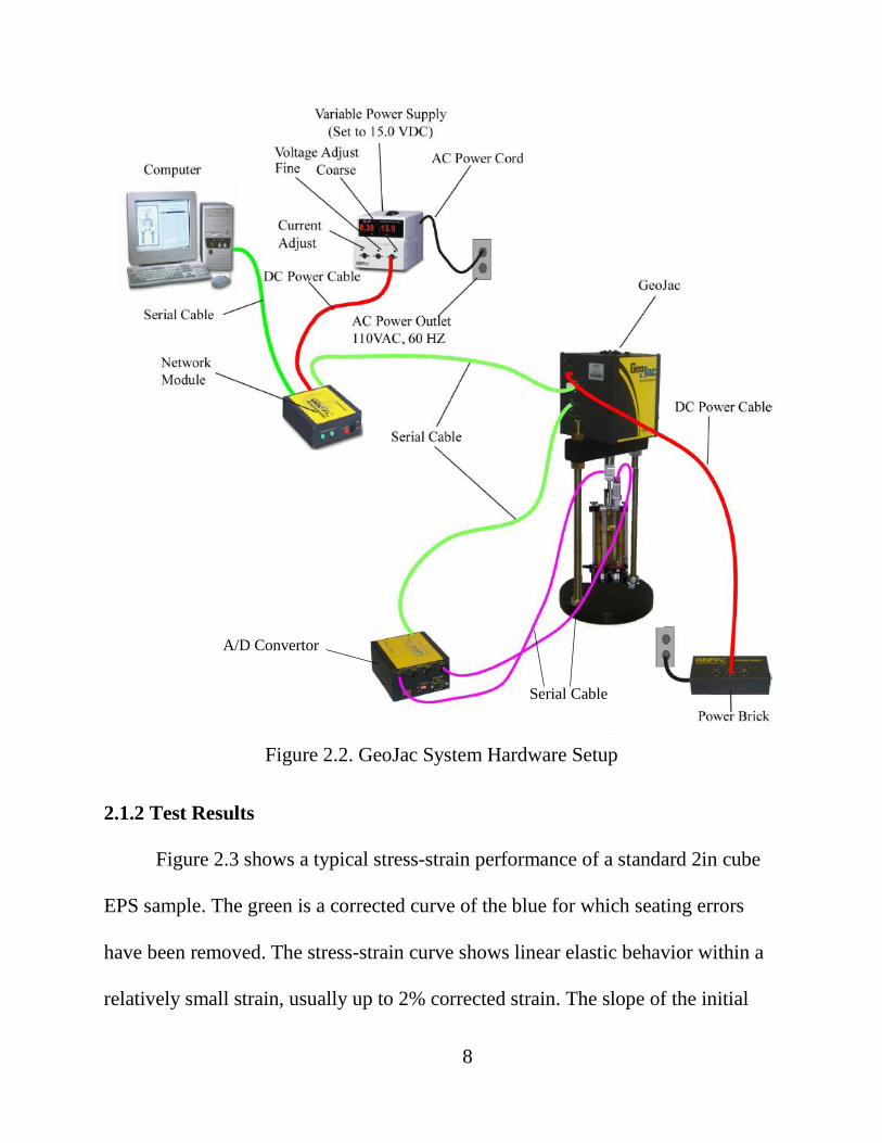
Figure 2.2. GeoJac System Hardware Setup
2.1.2 Test Results
Figure 2.3 shows a typical stress-strain performance of a standard 2in cube
EPS sample. The green is a corrected curve of the blue for which seating errors
have been removed. The stress-strain curve shows linear elastic behavior within a
relatively small strain, usually up to 2% corrected strain. The slope of the initial
A/D Convertor
Serial Cable
8
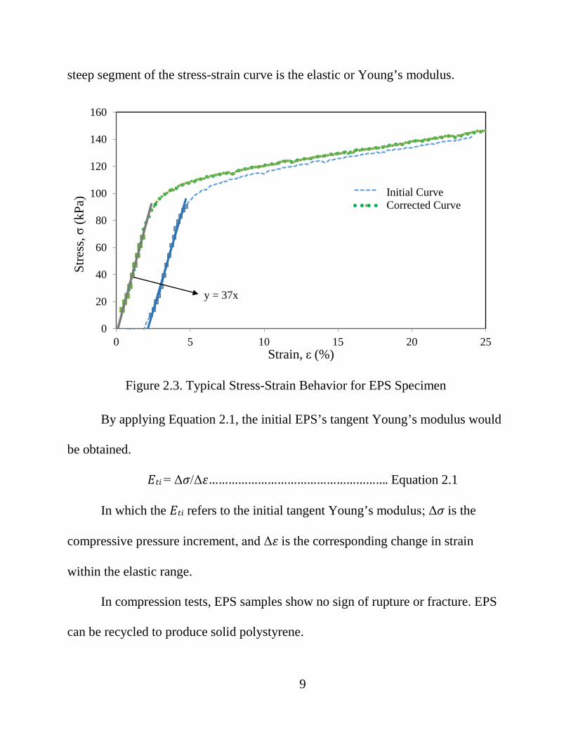
steep segment of the stress-strain curve is the elastic or Young’s modulus.
Figure 2.3. Typical Stress-Strain Behavior for EPS Specimen
By applying Equation 2.1, the initial EPS’s tangent Young’s modulus would
be obtained.
𝐸𝐸𝑡𝑡𝑖𝑖 = Δ𝜎𝜎/Δ𝜀𝜀………………………………………………. Equation 2.1
In which the 𝐸𝐸𝑡𝑡𝑖𝑖 refers to the initial tangent Young’s modulus; Δ𝜎𝜎 is the
compressive pressure increment, and Δ𝜀𝜀 is the corresponding change in strain
within the elastic range.
In compression tests, EPS samples show no sign of rupture or fracture. EPS
can be recycled to produce solid polystyrene.
y = 37x
0
20
40
60
80
100
120
140
160
0 5 10 15 20 25
Stre
ss, σ
(kPa
)
Strain, ε (%)
Series1
Series3Initial Curve Corrected Curve
9
2.2 EPS Properties
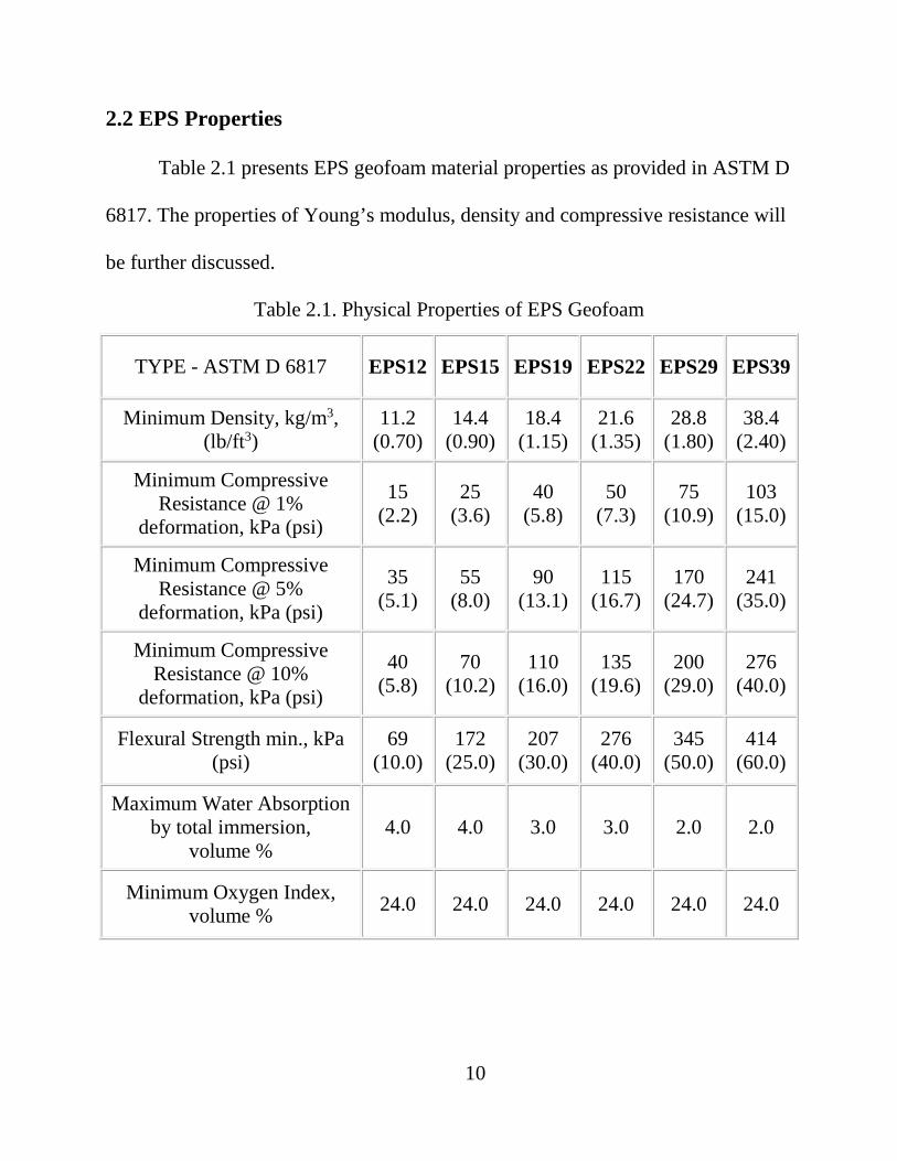
Table 2.1 presents EPS geofoam material properties as provided in ASTM D
6817. The properties of Young’s modulus, density and compressive resistance will
be further discussed.
Table 2.1. Physical Properties of EPS Geofoam
TYPE - ASTM D 6817 EPS12 EPS15 EPS19 EPS22 EPS29 EPS39
Minimum Density, kg/m3, (lb/ft3)
11.2 (0.70)
14.4 (0.90)
18.4 (1.15)
21.6 (1.35)
28.8 (1.80)
38.4 (2.40)
Minimum Compressive Resistance @ 1%
deformation, kPa (psi)
15 (2.2)
25 (3.6)
40 (5.8)
50 (7.3)
75 (10.9)
103 (15.0)
Minimum Compressive Resistance @ 5%
deformation, kPa (psi)
35 (5.1)
55 (8.0)
90 (13.1)
115 (16.7)
170 (24.7)
241 (35.0)
Minimum Compressive Resistance @ 10%
deformation, kPa (psi)
40 (5.8)
70 (10.2)
110 (16.0)
135 (19.6)
200 (29.0)
276 (40.0)
Flexural Strength min., kPa (psi)
69 (10.0)
172 (25.0)
207 (30.0)
276 (40.0)
345 (50.0)
414 (60.0)
Maximum Water Absorption by total immersion,
volume % 4.0 4.0 3.0 3.0 2.0 2.0
Minimum Oxygen Index, volume % 24.0 24.0 24.0 24.0 24.0 24.0
10

2.2.1 Young’s Modulus
Young’s modulus of EPS is important for design with geofoam. The
Young’s modulus of EPS samples is usually obtained from the unconfined
compression testing of cubic or cylindrical specimens. More often, Young’s
modulus values are obtained from unconfined compression tests on 50mm cube
specimens in accordance with ASTM D 1621, C 165, EN 826 or ISO 844.
Duškov (1990) reported back-calculated elastic modulus of EPS geofoam
from impulsive force, was between 13MPa and 34MPa, much higher than 5MPa
achieved from unconfined compression tests. Investigations of 20kg/m³ density
EPS at low temperatures, freezing/thawing cycles and potential moisture
absorption have not shown significant effects on EPS behavior. Srirajan (2001)
reported that both initial Young's modulus and post-yield modulus of EPS blocks
increase with density for traditional 50mm cube specimens. With increasing
ambient stress, the initial Young’s modulus and the post-yield modulus can
decrease. Changes in initial modulus with increasing density reported in previous
investigations are shown in Figure 2.4 (Eriksson and Trank, 1991; Horvath, 1995;
Van Dorp, 1996; BASF, 1997; Sun, 1997; Duskov, 1997; Elragi, 2000; Anasthas,
2001). For design of roads on EPS subgrades, a modulus of 5MPa is commonly
used (Negussey, 2007).
11
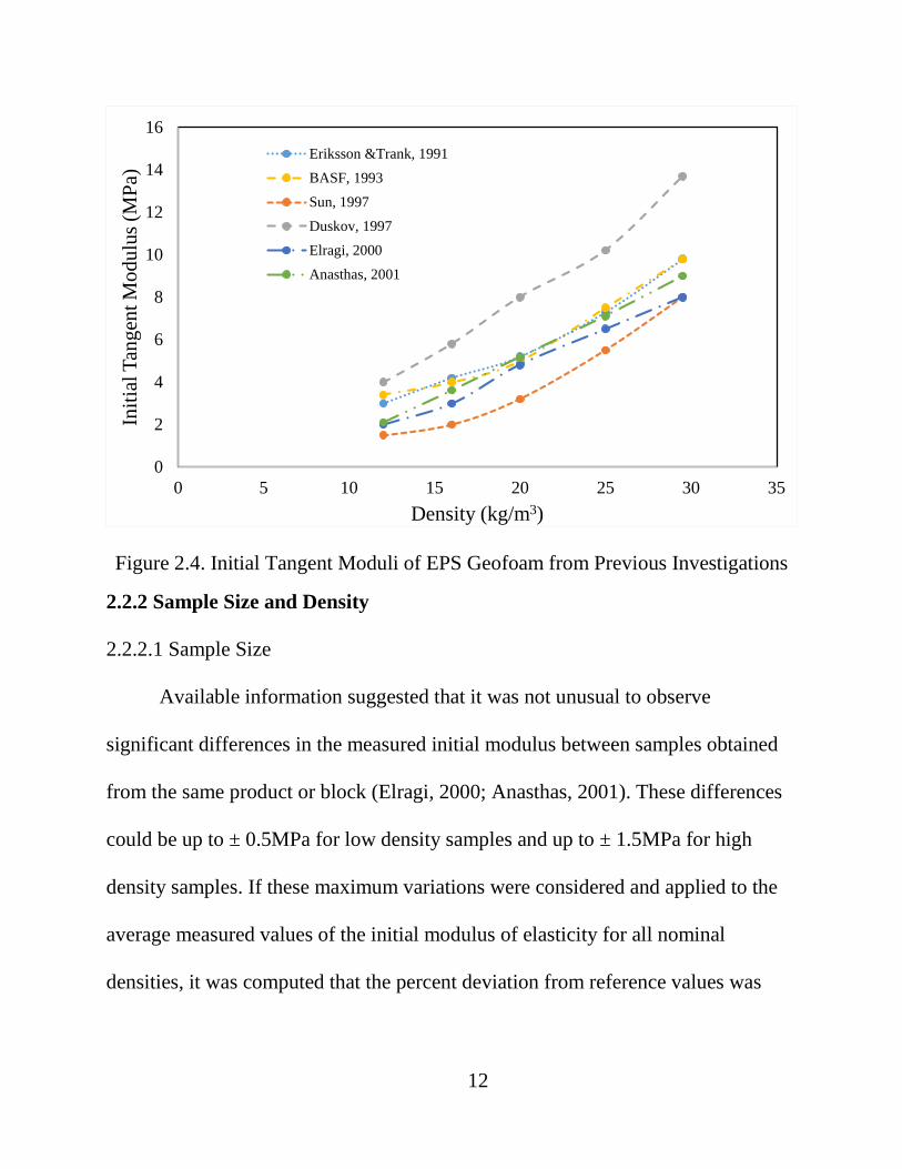
Figure 2.4. Initial Tangent Moduli of EPS Geofoam from Previous Investigations
2.2.2 Sample Size and Density
2.2.2.1 Sample Size
Available information suggested that it was not unusual to observe
significant differences in the measured initial modulus between samples obtained
from the same product or block (Elragi, 2000; Anasthas, 2001). These differences
could be up to ± 0.5MPa for low density samples and up to ± 1.5MPa for high
density samples. If these maximum variations were considered and applied to the
average measured values of the initial modulus of elasticity for all nominal
densities, it was computed that the percent deviation from reference values was
0
2
4
6
8
10
12
14
16
0 5 10 15 20 25 30 35
Initi
al T
ange
nt M
odul
us (M
Pa)
Density (kg/m3)
Eriksson &Trank, 1991BASF, 1993Sun, 1997Duskov, 1997Elragi, 2000Anasthas, 2001
12

between ± 25% and ± 40%. Accordingly, the significant increase in measured
initial modulus values could be attributed to the effect of sample size.
Elragi et al. (2000) evaluated the performance of EPS geofoam under
unconfined compression using traditional 50mm cubes, 600mm cubes and
cylindrical samples of 76mm diameter with density of 15 and 29kg/m3,
respectively. The traditional 50mm cube samples significantly over-estimated
initial deformations and thus underestimated Young’s modulus values for geofoam,
which may have partly resulted from the crushing and damage near the EPS block
and rigid plate loading interfaces. In the large cubic EPS as well as cylindrical
samples, vertical deformation was also observed for gauge length in the middle
third of the height. The results indicated that the distribution of vertical strains over
the height of geofoam block was not uniform. The segment on top of the EPS
block had the lowest modulus of 1.2MPa. The end parts of the specimen were
more severely deformed than the mid-segment of the EPS block. The major reason
of the relatively high deformation of the small scale samples should be attributed to
the seating and the end effects near the geofoam and rigid plate-loading interface.
The values of Poisson’s Ratio of small samples were relatively low compared with
the results from large size blocks. Atmatzidis (2001) tested the EPS blocks with the
transverse section of 100mm×100mm and the various aspect ratio of 0.5, 1.0 and
2.0. According to Atmatzidis (2001), the shape, size and the aspect ratio of EPS
13

geofoam specimens that were checked in the unconfined compression test showed
comparatively little effects on the yield pressure and compression resistance.
However, shape, size and the aspect ratio of EPS geofoam seemed to have some
impacts on the initial elastic modulus. It would achieve comparatively higher
initial modulus when the size of the specimen was larger than the traditional 50mm
cubes. If the test results of 50mm cubes were taken into designing, the developed
strains or deformation would likely be overestimated by a factor of 2. Eriksson and
Trank (1991) suggested a suitable dimension of EPS blocks would be 200×200×t/3
mm, where t/3 is the thickness of the specimen and t is the thickness of the whole
large block.
The size of the specimens also will greatly influence the creep performance
of the EPS blocks. As the specimen size increases, the stiffness of EPS also
increases leading to a decrease in creep. Apart from the size of the samples,
previous results also indicated that the modulus and strength of EPS depend on the
loading rate. The standard loading rate used in ASTM D 6817 is 10% strain per
minute. Awol (2012) indicted that decreasing loading rate has a tendency of
increasing initial tangent modulus.
2.2.2.2 Density
The density of EPS geofoam material is regarded as the major indicator of
behavior. EPS material is mostly made up of air-filled space. The air space of the
14

geofoam material is approximately 98% of the block volume, the density of the
material is low. The densities of EPS geofoam vary between 12 and 30 kg/m3,
among which the 20kg/m3 (1.25pcf) is the most widely used for civil engineering
applications (Lingwall, 2011). According to Negussey (2007), the initial modulus
of EPS samples with 20kg/m3 density is 5MPa, which is in the range normally
associated with very soft to soft clays (Das, 1998) when compared to typical
design values with different types of soil. The performance of EPS geofoam with a
density of 24kg/m3 showed that over 8MPa modulus implied by field data and
were better with stiffer clays (Negussey, 2007). While the modulus of about 8 to
10MPa for bigger samples of 32kg/m3 density geofoam was in better agreement
with the modulus estimates from field observations of 32kg/m3 density EPS. When
used for other purposes, insulation for example, the denser EPS is slightly better
although XPS may be preferred (van Dorp, 1988). EPS geofoam is much lighter
and easier to handle than soil, rock and other fill materials that are widely used in
conventional geotechnical constructions.
According to the survey of Eriksson and Trank (1991), the bulk density may
vary within the EPS blocks. Therefore, the samples tested should be selected from
the EPS blocks by taking the variation in bulk density into consideration. The same
amount of samples should be selected for testing from the upper layer, center layer
15
and lower layer together. There is no evidence that indicates the density of EPS is
affected by the age of EPS material.
The price of resin and then EPS blocks increase with the price of oil and the
EPS density. For large volume use of EPS, more savings can be realized with low
density EPS. Figure 2.4 indicates the initial modulus increase with the increase of
EPS densities from previous investigations. The stress-strain relationships are
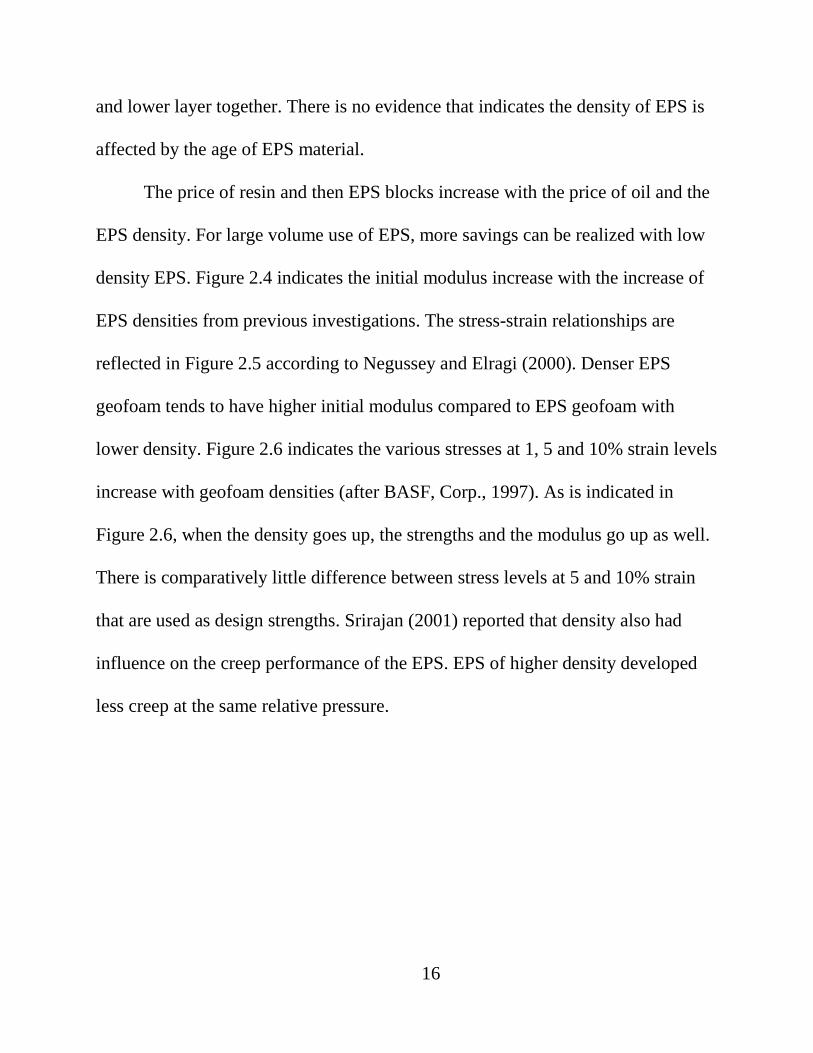
reflected in Figure 2.5 according to Negussey and Elragi (2000). Denser EPS
geofoam tends to have higher initial modulus compared to EPS geofoam with
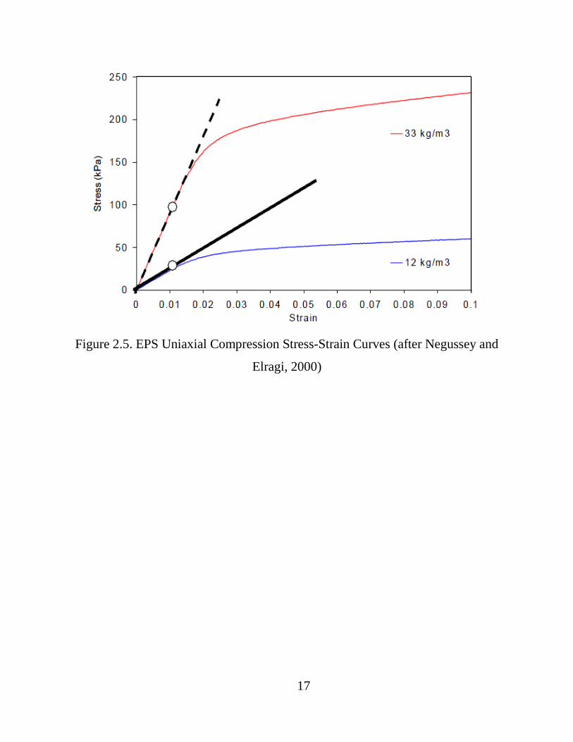
lower density. Figure 2.6 indicates the various stresses at 1, 5 and 10% strain levels
increase with geofoam densities (after BASF, Corp., 1997). As is indicated in
Figure 2.6, when the density goes up, the strengths and the modulus go up as well.
There is comparatively little difference between stress levels at 5 and 10% strain
that are used as design strengths. Srirajan (2001) reported that density also had
influence on the creep performance of the EPS. EPS of higher density developed
less creep at the same relative pressure.
16
Strain
Figure 2.5. EPS Uniaxial Compression Stress-Strain Curves (after Negussey and
Elragi, 2000)
17
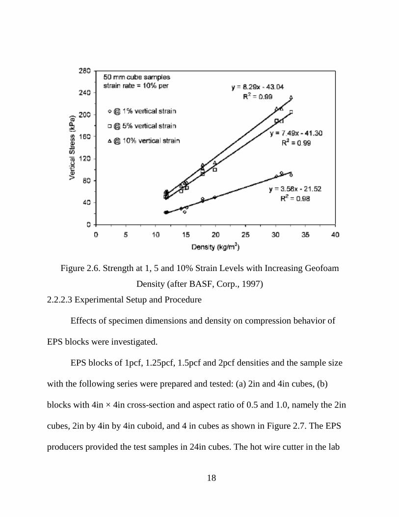
Figure 2.6. Strength at 1, 5 and 10% Strain Levels with Increasing Geofoam
Density (after BASF, Corp., 1997)
2.2.2.3 Experimental Setup and Procedure
Effects of specimen dimensions and density on compression behavior of
EPS blocks were investigated.
EPS blocks of 1pcf, 1.25pcf, 1.5pcf and 2pcf densities and the sample size
with the following series were prepared and tested: (a) 2in and 4in cubes, (b)
blocks with 4in × 4in cross-section and aspect ratio of 0.5 and 1.0, namely the 2in
cubes, 2in by 4in by 4in cuboid, and 4 in cubes as shown in Figure 2.7. The EPS
producers provided the test samples in 24in cubes. The hot wire cutter in the lab
18
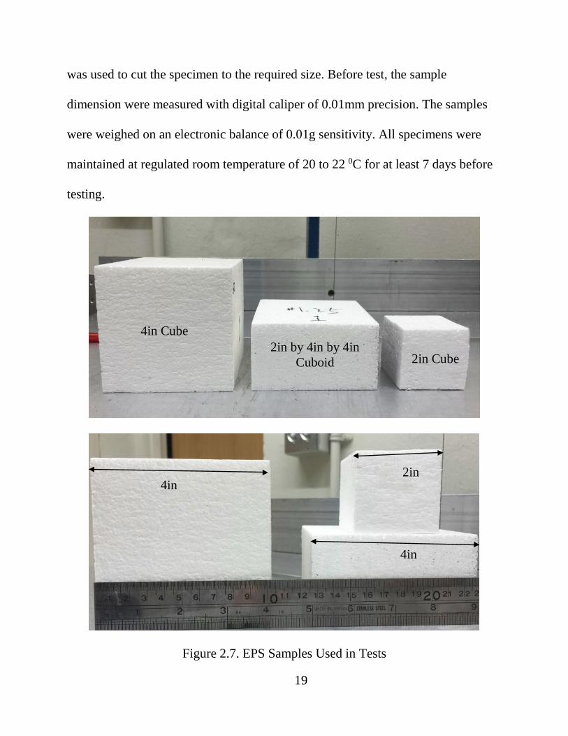
was used to cut the specimen to the required size. Before test, the sample
dimension were measured with digital caliper of 0.01mm precision. The samples
were weighed on an electronic balance of 0.01g sensitivity. All specimens were
maintained at regulated room temperature of 20 to 22 0C for at least 7 days before
testing.
Figure 2.7. EPS Samples Used in Tests
2in by 4in by 4in Cuboid
4in Cube
2in Cube
4in 2in
4in
19
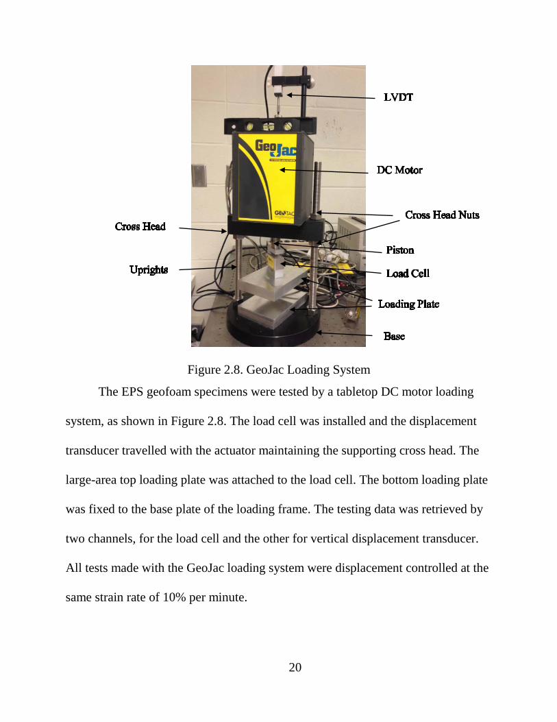
Figure 2.8. GeoJac Loading System
The EPS geofoam specimens were tested by a tabletop DC motor loading
system, as shown in Figure 2.8. The load cell was installed and the displacement
transducer travelled with the actuator maintaining the supporting cross head. The
large-area top loading plate was attached to the load cell. The bottom loading plate
was fixed to the base plate of the loading frame. The testing data was retrieved by
two channels, for the load cell and the other for vertical displacement transducer.
All tests made with the GeoJac loading system were displacement controlled at the
same strain rate of 10% per minute.
20

2.2.2.4 Test Results
Unconfined compression tests were conducted in order to evaluate the effect
of sample geometry and densities on the observed behavior of the EPS geofoam. A
minimum of two samples were tested for each test combination and all the stress-
strain curves and strength values were obtained for each block. The stress-strain
curves were corrected at very low strain levels in order to exclude seating errors.
2.2.2.4.1 Test Results of Sample Size
Figure 2.9. Sample Size Effect on Moduli for 2 and 4in Cubes
According to the lab tests, the strengths of 2in cube EPS geofoam were all
relatively smaller than bigger cubic samples, which means that the size of the
samples affect the strength of EPS regardless of the density. As for the samples
y = 0.005x + 2.9
y = 0.015x + 3.2
y = 0.022x + 4.2
y = 0.012x + 7.1
0
1
2
3
4
5
6
7
8
9
0 10 20 30 40 50 60 70 80
Mod
ulus
(MPa
)
Sample Volume (in3)
1 pcf1.25pcf1.5pcf2pcf
2in Cube Samples 4in Cube Samples
21
with an aspect ratio of 1, namely the 2in cube and 4in cube samples, the initial
modulus of EPS blocks increased with the increase of sample size, as shown in
Figure 2.9. For all nominal densities tested, the 4in cube samples had a 10% higher
initial modulus than the 2in cube samples.
The previous investigations (Eriksson and Trank, 1991; van Dorp, 1996;
Elragi, 2000) showed the large sample based modulus could be almost double that
of the small sample of the same density due to end effects of surface between the
loading plate and the sample. But for the tests that were presented in this
investigation, the variations in the sizes of the samples were not significant, and
this might be one reason that the differences of the modulus of the different size
samples were not obvious. The tests done by Negussey (2007) with a height of
24in cube samples showed that, due to the 24in cube samples were closer to the
thickness of common full size EPS blocks, the modulus of about 10MPa for the
24in cube samples agreed better with the modulus estimated with field observation.
The modulus values derived from laboratory tests on small size samples were too
small or too unrealistic to be used directly in the field design. A possible
explanation is that the end effects would be proportionally more significant for
small-sized samples and could cause large differences in modulus obtained from
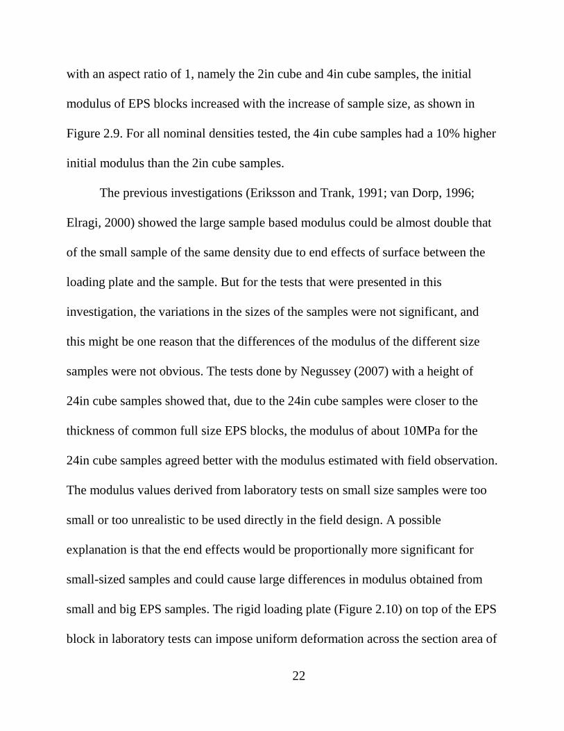
small and big EPS samples. The rigid loading plate (Figure 2.10) on top of the EPS
block in laboratory tests can impose uniform deformation across the section area of
22
test samples. According to Taylor (1948), rigid loading plate would produce higher
stresses toward the edges of samples. The average deformation near the rigid
loading plate was shown to be higher than the deformations across the geofoam to
geofoam interfaces according to Elragi (2000). With development of image
analysis processes, an alternative means for measuring and investigating the
interface pressure distributions becomes possible. This will be discussed in a later
chapter.
Figure 2.10. Load Cell and Top Loading Plate
Figure 2.11. Comparison of Moduli for Different Aspect Ratio
y = 1.4x + 1.7
y = 2.9x + 1.2
y = 3.13x + 1.7
y = 5.2x + 2.4
0
1
2
3
4
5
6
7
8
9
0 0.5 1 1.5
Mod
ulus
(MPa
)
Aspect Ratio
1 pcf1.25pcf1.5pcf2pcf
23

The results obtained from tests on 4in cubes (aspect ratio is 1) and results
obtained from the prisms with 4in×4in cross-section and 2in height for aspect ratio
equal to 0.5 are shown in Figure 2.11. A reduction of the aspect ratio from 1.0 to
0.5 resulted in decrease of elastic modulus by 15% for 1pcf to 60% for 2pcf
density.
2.2.2.4.2 Test Results of Density
The stress-strain curves for different densities of 2in cube samples are shown
in Figure 2.12. The stress-strain behaviors of all the density types are very similar.
It clearly shows that the initial modulus of EPS blocks increases with density, so
does yield. The samples with densities of 2pcf are stiffer than the 1pcf and 1.5pcf
EPS and the 1pcf ones are the softest. All the EPS blocks yield at about the same
strain level, which is around 2.2%.
24

Figure 2.12. Stress-Strain Distribution Curves from Traditional Testing of 2in
Cube Samples
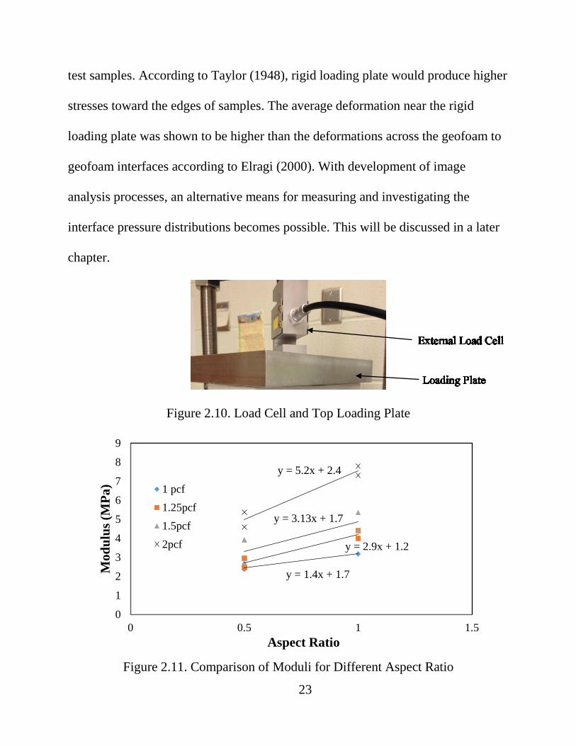
All results obtained from unconfined compression tests on 2in and 4in cubes
and 4in×2in×4in prisms are presented in Figure 2.13. According to Figure 2.13,
the initial modulus of the EPS geofoam increases with the increase of EPS
densities for all the sample sizes. The moduli of 1pcf (16kg/m3), 1.25pcf (20kg/m3),
1.5pcf (24kg/m3) and 2pcf (32kg/m3) density EPS are all relatively lower than the
values obtained from ASTM D 8617.
0
40
80
120
160
200
240
0 3 6 9 12 15
Stre
ss (k
Pa)
Strain (%)
2pcf, E1=7.0MPa1.5pcf, E2=4.4MPa1.25pc, E3=3.5MPa1pcf, E4=2.0MPa
2.2
E1
E2
E4
E3
2pcf, E1=7.0MPa 1.5pcf, E2=4.4MPa 1.25pcf, E3=3.5MPa 1pcf, E4=2.0MPa
25
Figure 2.13. Moduli of EPS with Different Densities
2.2.2.5 Conclusions
1. The sample size and density affect the strength of EPS samples as was
also suggested by (Eriksson and Trank, 1991; Horvath, 1995; van Dorp, 1996;
Elragi, 2000; Atmatzidis, 2001; Awol, 2012). The foregoing information and
observations indicate that, in addition to the anticipated scatter of data due to
density deviation from nominal values, the results of unconfined compression test
are affected by the size as well as by the aspect ratio of the samples tested. The
bigger samples have larger modulus than smaller ones and the EPS with higher
density have higher strength than the EPS with lower density.
y = 0.2497x - 0.9214
y = 0.1537x + 0.1761
y = 0.3224x - 1.9997
0
1
2
3
4
5
6
7
8
9
0 5 10 15 20 25 30 35 40
Mod
ulus
(MPa
)
Density (kg/m3)
2 by 2 by 2
4 by 2 by 4
4 by 4 by 4
26
2. Shape, size and aspect ratio of EPS geofoam samples have relatively
insignificant effects on measured yield stress and compressive strength. However,
size and aspect ratio have a significant effect on the initial modulus of elasticity
which attains higher values (up to 100%) when the sample volume is one order of
magnitude larger than the conventional 2in cubes. When results from testing 2in
cubes are used for design purposes, expected strains or deformations may be
overestimated by a factor of 2.
3. Beyond adjustments for seating error, the reason for the noted significant
difference in modulus obtained from small and large size samples was assumed to
be due to end effects at the loading plate boundaries.
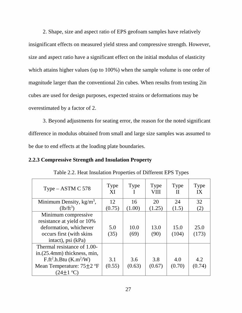
2.2.3 Compressive Strength and Insulation Property
Table 2.2. Heat Insulation Properties of Different EPS Types
Type – ASTM C 578 Type
XI Type
I Type VIII
Type II
Type IX
Minimum Density, kg/m3, (lb/ft3)
12 (0.75)
16 (1.00)
20 (1.25)
24 (1.5)
32 (2)
Minimum compressive resistance at yield or 10% deformation, whichever occurs first (with skins
intact), psi (kPa)
5.0 (35)
10.0 (69)
13.0 (90)
15.0 (104)
25.0 (173)
Thermal resistance of 1.00-in.(25.4mm) thickness, min,
F.ft2.h.Btu (K.m2/W) Mean Temperature: 75±2 oF
(24±1 oC)
3.1 (0.55)
3.6 (0.63)
3.8 (0.67)
4.0 (0.70)
4.2 (0.74)
27

In the US and Canada, ASTM C 578 (Table 2.2) presents EPS heat
insulation, thermal resistance, and the compressive strength for different densities
of EPS geofoam. The classification of EPS types for ASTM C 578 is slightly
different from ASTM D 6187 (Table 2.1).
In order to meet the requirements of the compressive strength that are
required in ASTM C 578, polystyrene heat insulation board offer compressive
resistance with 10% distortion when tested in conformity with the requirements of
ASTM D 1621. ASTM C 578 Type I material whose density is usually 0.9pcf is
the most appropriate material to be used in foundation or the construction of the
wall where the pressure requirements of the insulation values are the least.
According to the creep testing of geofoam specimens at various pressure levels, 50%
of the overall compression resistance was identified as the upper limit of
consideration working stress for designing with geofoam (Srirajan, 2001).
2.2.4 Creep Behavior
Creep is an important consideration for designing with EPS geofoam.
Sun (1997) performed creep tests on 50mm cube of average 18kg/m3 density
EPS geofoam using cantilever static loading system. For sustained pressure of 30%
of 85kPa compressive working strength at 5% strain, creep strain after 461days
were 0.8%, and for 50% strain were 3%, and for 70% the creep strain were 14.4%.
28
Compression loads of 30% or less would have little impact on the creep
deformation performance.
Duskov (1997) also did creep tests and achieved similar results from
cylindrical of geofoam samples. In the first set of experiments, a specimen with a
diameter of 200mm, height of 100mm and density of 20kg/m3 was tested with a
20kPa pressure. After 400days, the strain value was only 0.20% and most of the
strains happened in the very first day. In the second set, however, the specimen
with diameter of 100mm, height of 300mm and density of 15 and 20kg/m3 was
loaded to10kPa and 20kPa respectively. The result of the former (10kPa pressure)
was 0.25% and the later (20kPa pressure) was 0.5% after 400days. The instant
strains under the 20 and 10kPa were 0.3 and 0.15%, respectively. There was little
difference in the creep behavior with the two 15 and 20kg/m3 different specimen
densities.
Sheeley (2000) reported creep test results for 50mm cubes with 21kg/m3
density, and subjected to 30%, 50%, and 70% of compression strength at 5% strain.
The investigation showed that for 30% and 50% loading, the strain mostly
occurred in the first two days. For the sample loaded to 30% of compressive
strength, a total strain of 0.95% occurred in 500 days in which 66% was observed
in the first day. For the sample loaded at 50% compressive strength, a total strain
of 1.35% occurred in 500 days in which 68% was observed in the first day. For the
29
specimen loaded at 70% compression strength, there was much more creep
deformation and about 4% of the strain occurred in the first day. A total of 22%
strain occurred in the following 500days.
Working stress values are selected to limit creep deformations to acceptable
levels over the EPS service life. Creep is negligible if the initial strain does not
exceed 0.5% (Frydenlund and Aabøe 2001). At working stress level of less than 50%
of the yield, geofoam is found to have insignificant creep deformation (Negussey
and Jahanandish 1993).
Creep deformations are minimized or essentially avoided in most design
procedures by limiting allowable loads or surcharge pressures to below the
prescribed compressive strengths of the EPS geofoam (usually 30% of the strength
at 5 or 10% strain). A commonly used design approach developed in Norway is
based on limiting the allowable surcharge load over geofoam to 30% of the
compressive strength at 5% strain. If geofoam is exposed to loads greater than 50%
of the compressive strength at 5% strain, larger creep deformations occur.
30
CHAPTER 3
PRE-STRAIN INDUCED ANISOTROPY OF EPS GEOFOAM
The operation of heavy machinery or trucks during construction may result
in the pre-straining of EPS fills. Pre-straining of the EPS fills may also result from
seismic loading during an earthquake. In addition, improper working loads may
produce strains outside of the elastic range. In most embankment construction, EPS
blocks become subjected to higher level of stress during placement and compaction.
However, the effect of prior pre-stressing has not been closely investigated. It is of
great importance to closely understand the stress-strain behavior of EPS while
under cyclic loading within and outside of the elastic range. In this investigation,
EPS blocks of different densities were tested separately and in combination in
loading and reloading experiments. Comparison between densities and modulus
changes due to pre-strain history are examined.
3.1 Background
Use of EPS as a lightweight alternative material is widespread not only in
the US but also in other parts of the world. EPS geofoam is commonly installed
under pavement structures and over soft and compressible soils to minimize
settlements. However, unanticipated strains may exist either due to machine
operation during construction or confining stress effects. Stresses beyond the
elastic limit of EPS material would induce plastic strains and hence induce
31
anisotropy. Thus, the effect of such stress or strain anisotropy on EPS geofoam
performance should be investigated to appropriately design geofoam fills.
The design of EPS geofoam fill is based on the premise that strain induced
in the fill remains between 1 and 2 %. In addition, EPS geofoam is assumed to be
isotropic inherently. The property of EPS blocks was also found to show
anisotropy (Amsalu, 2014). Anisotropy is the property of being directionally
dependent, as opposed to isotropy which implies identical properties in all
directions. Anisotropy can be defined as a difference when measured along
different axes in the EPS material's physical or mechanical properties. Two
different forms of anisotropy in EPS geofoam can be distinguished, namely
inherent and induced.
Inherent anisotropy is an attribute acquired in the material manufacturing
process. Kutara et al. 1989 reported that specimens loaded perpendicular to the
direction of fabrication showed higher deviator stresses at failure than those loaded
parallel to the direction of fabrication. The compressibility of EPS geofoam is
highly affected by the shape of the cells. Cells close to the mold wall are usually
flattened due to the molding processes. If the compressive loads are applied
perpendicular to the direction of stretching, the flattened cells will be flattened
more and smaller values of compressive strength are obtained (BASF 1998).
Therefore, a higher bearing capacity can be expected if the foam is loaded
32

perpendicular to the direction of fabrication. This can be explained as the effect of
inherent anisotropy of EPS blocks. Isotropy is regardless of material dimension. If
there is inherent anisotropy, it tends to be small. Geofoam is generally considered
to be inherent isotropy.
Induced anisotropy is due to the strain associated with an applied stress. It is
hard to find a relatively easy experimental technique for demonstrating the degree
of anisotropy that exists at any loading level in EPS blocks. A separation of the
effects of inherent and induced anisotropy can be achieved by treating the
anisotropy of the original EPS material as the inherent anisotropy. The stress-strain
behavior of this original EPS sample can then be compared with another EPS
sample subjected to an identical stress path and then reloaded with or without
change in the principal stress direction. Here the effect of an unloading stress path
is not included. Defining the degree of anisotropy which exists on reloading is not
a simple matter of initial stiffness and volume compressibility exhibited on
reloading with different principal stress directions. The variation in modulus during
reloading is complex and indicates a varying persistence in the influence of the
anisotropy existing at the beginning of reloading. The purpose here is not primarily
to be quantitative, but rather to illustrate the effect of pre-loading, which may result
in the induced anisotropy on EPS geofoam. The effect of induced anisotropy on
33
EPS characteristics was investigated by compression tests conducted on pre-
stressed foam. The practical significance of induced anisotropy was also discussed.
3.2 Test Procedures
3.2.1 Tests on Exhumed Samples from Field
The I88 culvert at Carrs Creek in the town of Sydney, Delaware County, NY
collapsed during a flood in June 2006 and was rapidly reconstructed by using EPS
geofoam fill as light weight material. EPS geofoam of 20 kg/m3 (1.25pcf) density
was selected and placed on soil bedding over the culvert in three layers for 2.7m
height on the eastbound embankment and two layers for 1.8m on the westbound
embankment. A total of 3.3m of compacted soil and pavement was placed over the
geofoam in the east bound and 2.4m on the west bound. The settlement of the
reconstructed pavement on the culvert became evident shortly after the completion
of the construction and the EPS geofoam fill was eventually removed.
Laboratory tests were performed on fresh samples (Figure 3.1) with nominal
density of 20 kg/m3 (1.25pcf) provided by the geofoam supplier as well as on the
exhumed blocks recovered on removal of the geofoam fill. From the exhumed big
blocks, which were pre-strained, 2in cube samples were cut from the middle by
noting the orientation of pre-loading. All the unconfined compression tests were
done on 2in cube samples as per ASTM D 1621 maintaining a strain rate of 10%
per minute. Tests were done both in the same and orthogonal direction to the pre-
34
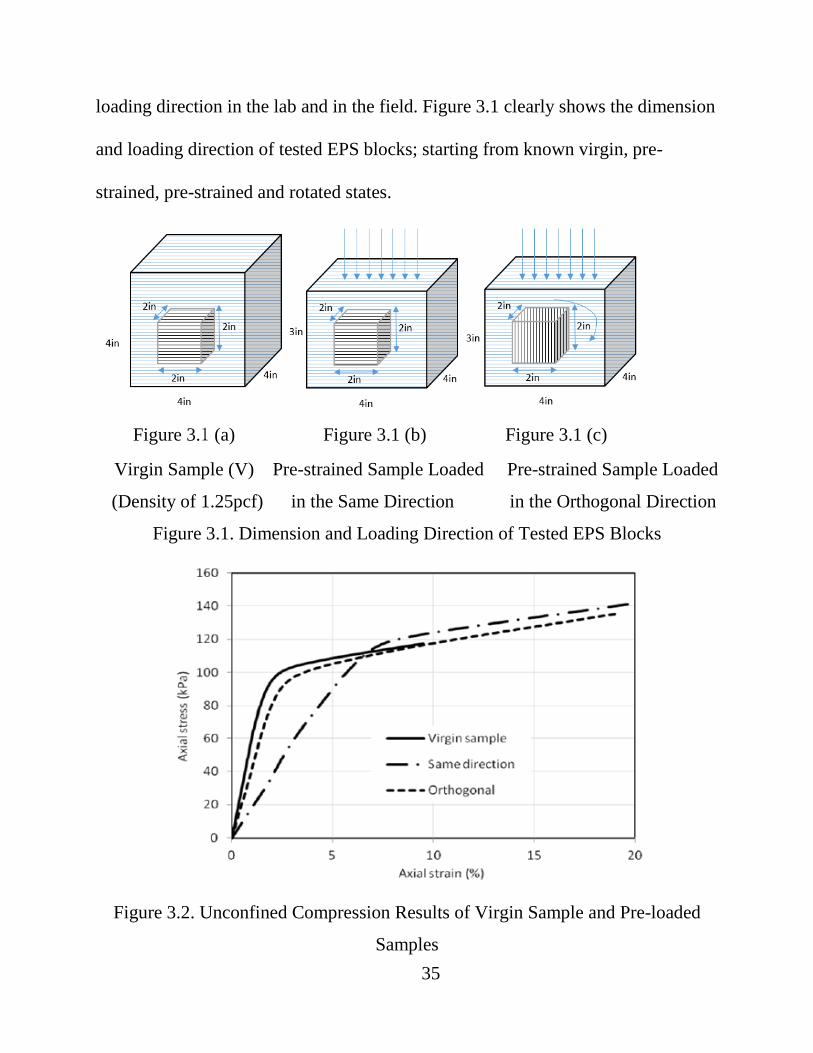
loading direction in the lab and in the field. Figure 3.1 clearly shows the dimension
and loading direction of tested EPS blocks; starting from known virgin, pre-
strained, pre-strained and rotated states.
Figure 3.1 (a) Figure 3.1 (b) Figure 3.1 (c)
Virgin Sample (V) Pre-strained Sample Loaded Pre-strained Sample Loaded
(Density of 1.25pcf) in the Same Direction in the Orthogonal Direction
Figure 3.1. Dimension and Loading Direction of Tested EPS Blocks
Figure 3.2. Unconfined Compression Results of Virgin Sample and Pre-loaded
Samples 35
The practical implications of tests on virgin samples and pre-strained to 10%
samples can be seen in Figure 3.2. The initial modulus of virgin sample and the
pre-strained sample loaded to the orthogonal direction are close. The pre-strain
EPS block has decreased initial modulus and lower work stress when loaded to the
same direction as pre-straining.
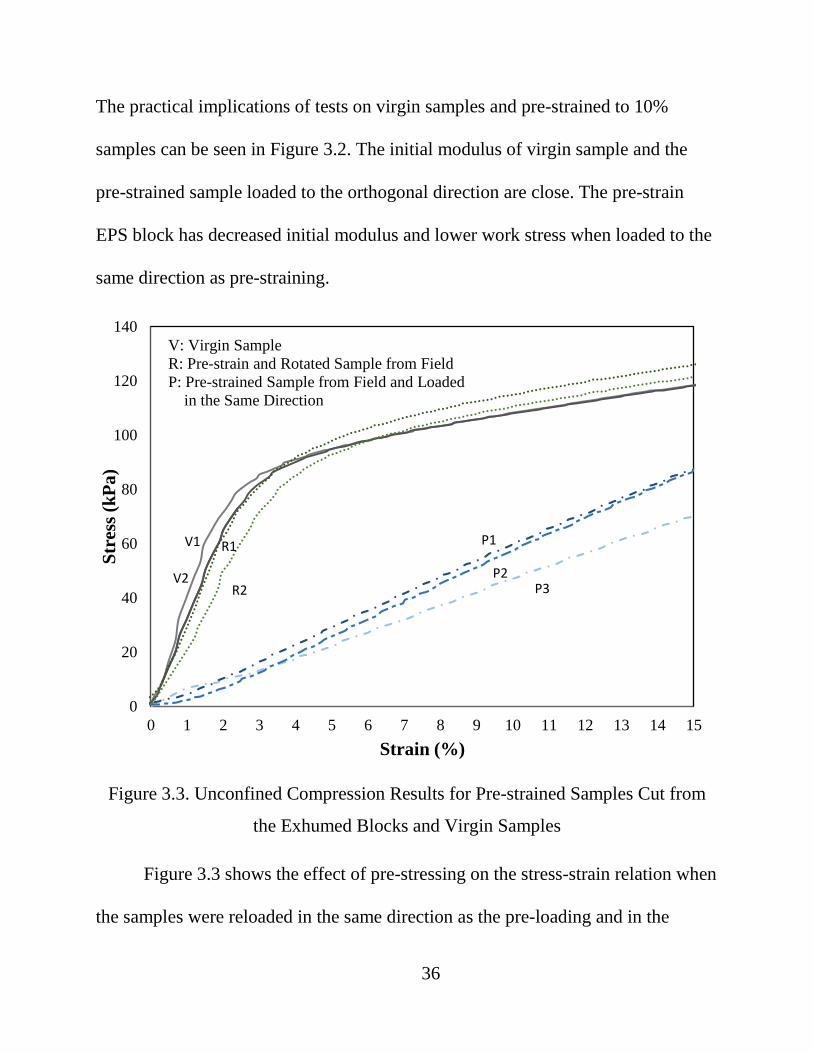
Figure 3.3. Unconfined Compression Results for Pre-strained Samples Cut from
the Exhumed Blocks and Virgin Samples
Figure 3.3 shows the effect of pre-stressing on the stress-strain relation when
the samples were reloaded in the same direction as the pre-loading and in the
0
20
40
60
80
100
120
140
0 1 2 3 4 5 6 7 8 9 10 11 12 13 14 15
Stre
ss (k
Pa)
Strain (%)
V1
V2
R1
R2
P1
P2P3
V: Virgin SampleR: Pre-strain and Rotated Sample from Field P: Pre-strained Sample from Field and Loaded
in the Same Direction
36

orthogonal direction to the pre-straining for the field samples from Carrs Creek.
The modulus ranges of the virgin samples, the pre-strained and rotated field
samples, and the pre-strained field samples who loaded in the same direction are
3.2~3.8MPa, 2.3~3.0MPa and 0.47~0.59MPa respectively. The compression stress
of the virgin samples, the pre-strained and rotated field samples, and the pre-
strained field samples that were loaded in the same direction at 1% strain are
34~41kPa, 21~28kPa and 2~6kPa respectively. The compression stress of the
virgin samples, the pre-strained and rotated field samples, and the pre-strained field
samples that were loaded in the same direction at 10% strain are 108kPa,
112~115kPa and 46~60kPa respectively. The test results reveal that the initial
modulus for loading in the pre-strained direction (P1, P2 and P3) were much lower
than for the samples loaded in the direction transverse (R1 and R2) to the pre-strain
and for virgin loading conditions (V1 and V2). The observation of inferior strengths
at 1% strain and strengths at 10% strain as for the pre-strained samples could be
attributed to the induced anisotropy that were caused by prior loading beyond yield,
and crushing of the EPS microstructure. The stress-strain curves of the tests that
were conducted in the orthogonal direction (R1 and R2) to the pre-straining
direction remained relatively unaffected, with just minor strength degradation
compared to the curves of virgin loading conditions (V1 and V2).
37
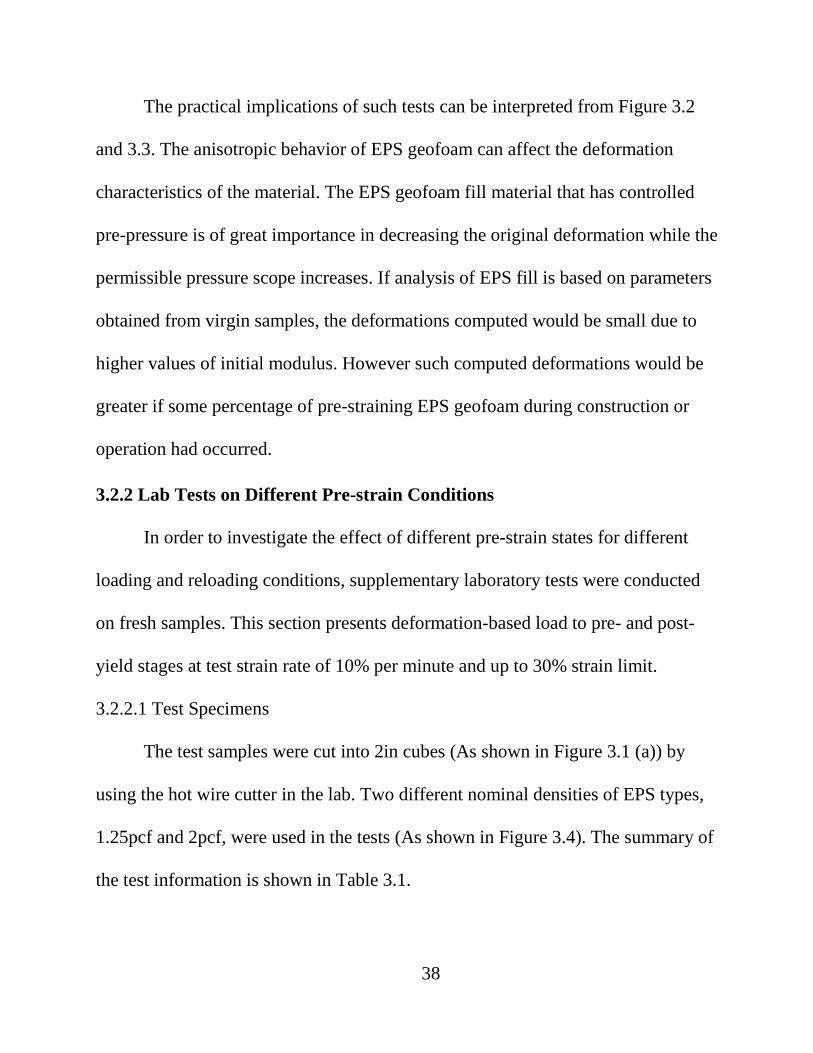
The practical implications of such tests can be interpreted from Figure 3.2
and 3.3. The anisotropic behavior of EPS geofoam can affect the deformation
characteristics of the material. The EPS geofoam fill material that has controlled
pre-pressure is of great importance in decreasing the original deformation while the
permissible pressure scope increases. If analysis of EPS fill is based on parameters
obtained from virgin samples, the deformations computed would be small due to
higher values of initial modulus. However such computed deformations would be
greater if some percentage of pre-straining EPS geofoam during construction or
operation had occurred.
3.2.2 Lab Tests on Different Pre-strain Conditions
In order to investigate the effect of different pre-strain states for different
loading and reloading conditions, supplementary laboratory tests were conducted
on fresh samples. This section presents deformation-based load to pre- and post-
yield stages at test strain rate of 10% per minute and up to 30% strain limit.
3.2.2.1 Test Specimens
The test samples were cut into 2in cubes (As shown in Figure 3.1 (a)) by
using the hot wire cutter in the lab. Two different nominal densities of EPS types,
1.25pcf and 2pcf, were used in the tests (As shown in Figure 3.4). The summary of
the test information is shown in Table 3.1.
38

1.25pcf (Type VIII) 2pcf (Type IX) EPS
Figure 3.4. 1.25pcf (Type VIII) and 2pcf (Type IX) EPS Blocks Used in Tests
Table 3.1. Test Information for the EPS Samples
Test Parameters
Sample Dimension 2in×2in×2in
EPS Type (Density, pcf) VIII (1.25) IX (2)
Test Strain Rate 10%/min
Test Strain Limit 30%
3.2.2.2 Tests Program
Different loading and reloading methods were used to investigate the pre-
strain effects on EPS strength for both 1.25 and 2pcf densities. The test programs
were set as the following three types: 1) Load/Unload and reload cycles were
39
performed in the pre-yield stages; 2) Load post yield to 30% strain before full
unloading and reloading cycles; 3) Load post yield to 30% strain before applying
partial unloading and reloading cycles.
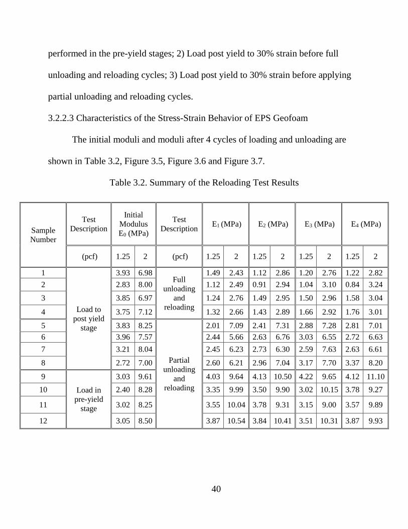
3.2.2.3 Characteristics of the Stress-Strain Behavior of EPS Geofoam
The initial moduli and moduli after 4 cycles of loading and unloading are
shown in Table 3.2, Figure 3.5, Figure 3.6 and Figure 3.7.
Table 3.2. Summary of the Reloading Test Results
Sample Number
Test Description
Initial Modulus E0 (MPa)
Test Description E1 (MPa) E2 (MPa) E3 (MPa) E4 (MPa)
(pcf) 1.25 2 (pcf) 1.25 2 1.25 2 1.25 2 1.25 2
1
Load to post yield
stage
3.93 6.98 Full
unloading and
reloading
1.49 2.43 1.12 2.86 1.20 2.76 1.22 2.82 2 2.83 8.00 1.12 2.49 0.91 2.94 1.04 3.10 0.84 3.24
3 3.85 6.97 1.24 2.76 1.49 2.95 1.50 2.96 1.58 3.04
4 3.75 7.12 1.32 2.66 1.43 2.89 1.66 2.92 1.76 3.01
5 3.83 8.25
Partial unloading
and reloading
2.01 7.09 2.41 7.31 2.88 7.28 2.81 7.01 6 3.96 7.57 2.44 5.66 2.63 6.76 3.03 6.55 2.72 6.63 7 3.21 8.04 2.45 6.23 2.73 6.30 2.59 7.63 2.63 6.61
8 2.72 7.00 2.60 6.21 2.96 7.04 3.17 7.70 3.37 8.20
9
Load in pre-yield
stage
3.03 9.61 4.03 9.64 4.13 10.50 4.22 9.65 4.12 11.10 10 2.40 8.28 3.35 9.99 3.50 9.90 3.02 10.15 3.78 9.27
11 3.02 8.25 3.55 10.04 3.78 9.31 3.15 9.00 3.57 9.89
12 3.05 8.50 3.87 10.54 3.84 10.41 3.51 10.31 3.87 9.93
40

Figure 3.5 (1). Stress-Strain Curves for 1.25pcf EPS
Figure 3.5. Unconfined Compression Test for Load and Unload
In/Near Pre-yield Stages
y = 30.3x y = 40.3x
y = 41.3x
y = 42.2x
y = 41.2x
0
20
40
60
80
100
120
0 0.5 1 1.5 2
Stre
ss (k
Pa)
Strain (%)
y = 23.9x
y = 33.4x
y = 35.0x
y = 30.1xy = 37.8x
0
20
40
60
80
100
120
0 0.5 1 1.5 2 2.5
Stre
ss (k
Pa)
Strain (%)
41
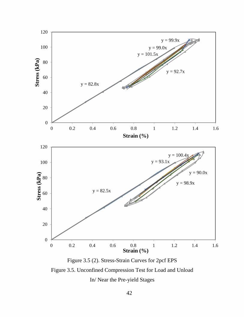
Figure 3.5 (2). Stress-Strain Curves for 2pcf EPS
Figure 3.5. Unconfined Compression Test for Load and Unload
In/ Near the Pre-yield Stages
y = 82.8x
y = 99.9xy = 99.0x
y = 101.5x
y = 92.7x
0
20
40
60
80
100
120
0 0.2 0.4 0.6 0.8 1 1.2 1.4 1.6
Stre
ss (k
Pa)
Strain (%)
y = 82.5x
y = 100.4xy = 93.1x
y = 90.0x
y = 98.9x
0
20
40
60
80
100
120
0 0.2 0.4 0.6 0.8 1 1.2 1.4 1.6
Stre
ss (k
Pa)
Strain (%)
42
Figure 3.5 is the stress-strain plot for four cycles of unloading and reloading
to near yield (1-2%) at strain rate of 10%/minute for both 1.25 and 2pcf geofoam
densities. The load and unload cycles were near yield and in pre-yield stages. The
cyclic loading and unloading did not change the initial modulus of elasticity. This
suggests EPS geofoam behaved elastically when the axial strain limit remained
below 2%. Similar conclusions were obtained from previous researches. Flaate
(1987) reported cyclic loading tests on EPS geofoam withstood an unlimited
number of cyclic loads as long as the loads were below 80% of the compressive
strength. Van Dorp (1988) also reported that there was no change in the initial
tangent modulus when a 20kg/m3 EPS was subjected to 2 million cycles of
straining between 0 and 1% at a cyclic strain rate of 10Hz.
43
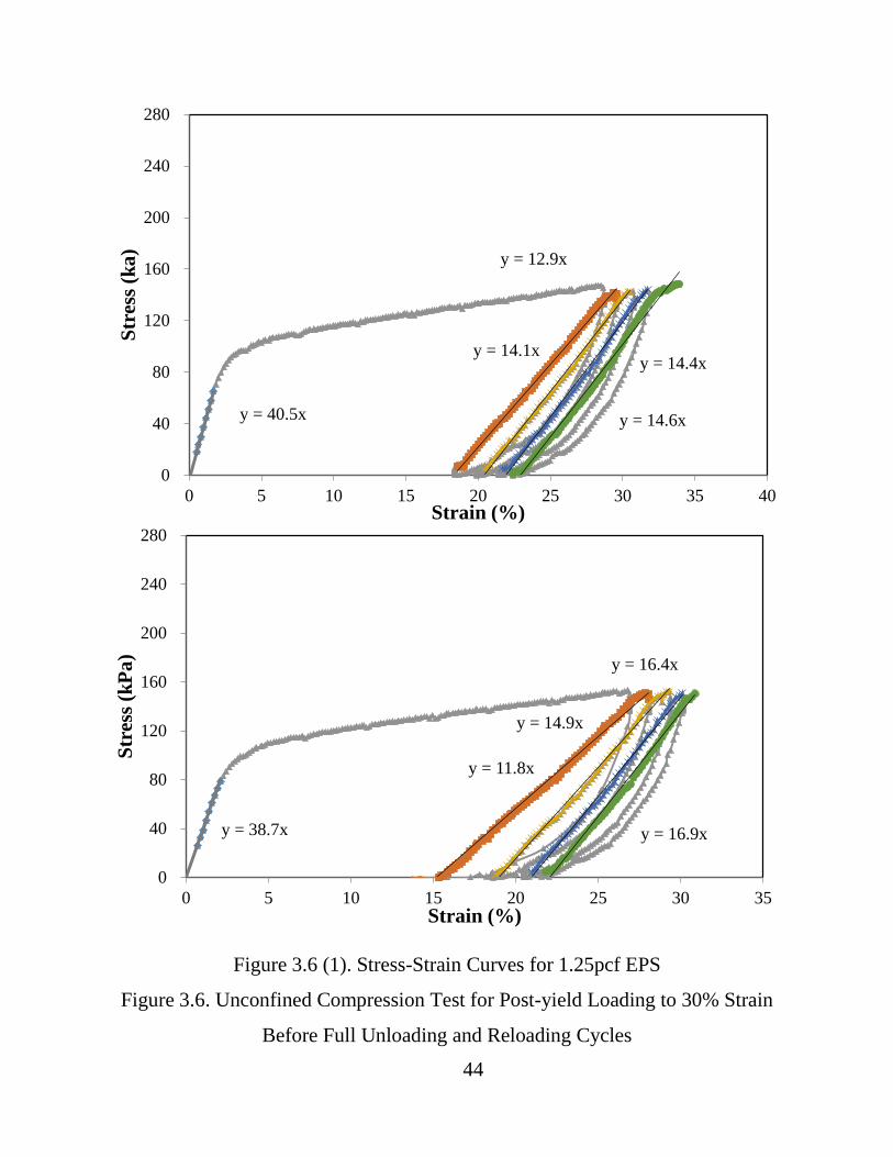
Figure 3.6 (1). Stress-Strain Curves for 1.25pcf EPS
Figure 3.6. Unconfined Compression Test for Post-yield Loading to 30% Strain
Before Full Unloading and Reloading Cycles
y = 40.5x
y = 12.9x
y = 14.1x
y = 14.6x
y = 14.4x
0
40
80
120
160
200
240
280
0 5 10 15 20 25 30 35 40
Stre
ss (k
a)
Strain (%)
y = 38.7x
y = 11.8x
y = 14.9x
y = 16.4x
y = 16.9x
0
40
80
120
160
200
240
280
0 5 10 15 20 25 30 35
Stre
ss (k
Pa)
Strain (%)
44

Figure 3.6 (2). Stress-Strain Curves for 2pcf EPS
Figure 3.6. Unconfined Compression Test for Post-yield Loading to 30% Strain
Before Full Unloading and Reloading Cycles
y = 69.8x
y = 24.3x
y = 28.6x
y = 27.6x
y = 28.2x
0
40
80
120
160
200
240
280
0 5 10 15 20 25 30 35
Stre
ss (k
Pa)
Strain (%)
y = 80.0x
y = 24.9x
y = 29.4x
y = 32.4x
y = 31.0x
0
40
80
120
160
200
240
280
0 5 10 15 20 25 30 35
Stre
ss (k
Pa)
Strain (%)
45
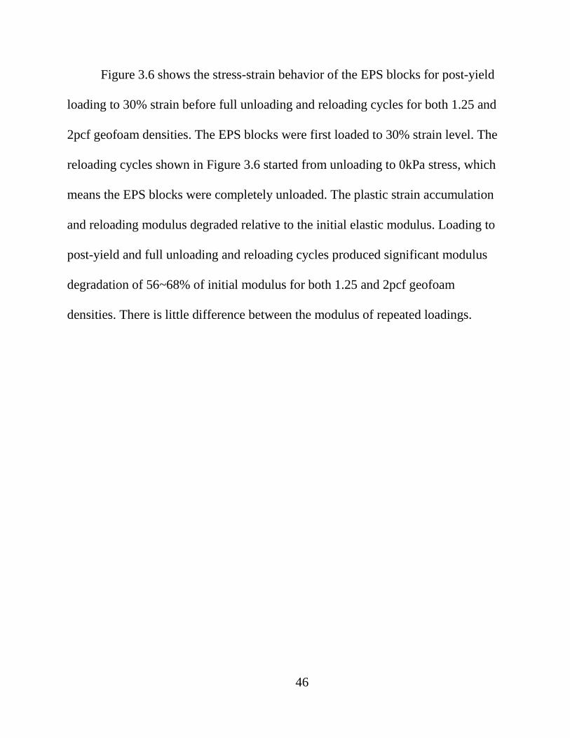
Figure 3.6 shows the stress-strain behavior of the EPS blocks for post-yield
loading to 30% strain before full unloading and reloading cycles for both 1.25 and
2pcf geofoam densities. The EPS blocks were first loaded to 30% strain level. The
reloading cycles shown in Figure 3.6 started from unloading to 0kPa stress, which
means the EPS blocks were completely unloaded. The plastic strain accumulation
and reloading modulus degraded relative to the initial elastic modulus. Loading to
post-yield and full unloading and reloading cycles produced significant modulus
degradation of 56~68% of initial modulus for both 1.25 and 2pcf geofoam
densities. There is little difference between the modulus of repeated loadings.
46

Figure 3.7 (1). Stress-Strain Curves for 1.25pcf EPS
Figure 3.7. Unconfined Compression Test for Post-yield Loading to 30% Strain
Before Partial Unloading and Reloading Cycles
y = 28.8x
y = 28.1x
y = 20.0x
y = 32.1x
0
40
80
120
160
200
240
280
0 5 10 15 20 25 30 35
Stre
ss (k
Pa)
Strain (%)
y = 31.7x
y = 25.9x y = 29.7x
0
40
80
120
160
200
240
280
0 5 10 15 20 25 30 35
Stre
ss (k
Pa)
Strain (%)
y = 24.1
y = 27.2 y = 27.1
47
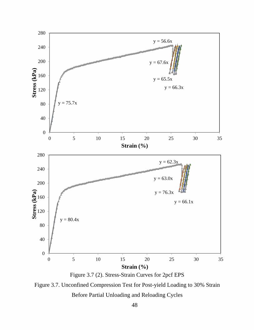
Figure 3.7 (2). Stress-Strain Curves for 2pcf EPS
Figure 3.7. Unconfined Compression Test for Post-yield Loading to 30% Strain
Before Partial Unloading and Reloading Cycles
y = 75.7x
y = 56.6x
y = 67.6x
y = 65.5x
y = 66.3x
0
40
80
120
160
200
240
280
0 5 10 15 20 25 30 35
Stre
ss (k
Pa)
Strain (%)
y = 80.4x
y = 62.3x
y = 63.0x
y = 76.3x
y = 66.1x
0
40
80
120
160
200
240
280
0 5 10 15 20 25 30 35
Stre
ss (k
Pa)
Strain (%)
48
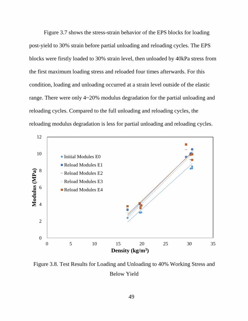
Figure 3.7 shows the stress-strain behavior of the EPS blocks for loading
post-yield to 30% strain before partial unloading and reloading cycles. The EPS
blocks were firstly loaded to 30% strain level, then unloaded by 40kPa stress from
the first maximum loading stress and reloaded four times afterwards. For this
condition, loading and unloading occurred at a strain level outside of the elastic
range. There were only 4~20% modulus degradation for the partial unloading and
reloading cycles. Compared to the full unloading and reloading cycles, the
reloading modulus degradation is less for partial unloading and reloading cycles.
Figure 3.8. Test Results for Loading and Unloading to 40% Working Stress and
Below Yield
0
2
4
6
8
10
12
0 5 10 15 20 25 30 35
Mod
ulus
(MPa
)
Density (kg/m3)
Initial Modules E0
Reload Modules E1
Reload Modules E2
Reload Modules E3
Reload Modules E4
49
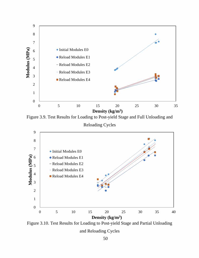
Figure 3.9. Test Results for Loading to Post-yield Stage and Full Unloading and
Reloading Cycles
Figure 3.10. Test Results for Loading to Post-yield Stage and Partial Unloading
and Reloading Cycles
0
1
2
3
4
5
6
7
8
9
0 5 10 15 20 25 30 35
Mod
ulus
(MPa
)
Density (kg/m3)
Initial Modules E0
Reload Modules E1
Reload Modules E2
Reload Modules E3
Reload Modules E4
0
1
2
3
4
5
6
7
8
9
0 5 10 15 20 25 30 35 40
Mod
ulus
(MPa
)
Density (kg/m3)
Initial Modules E0Reload Modules E1Reload Modules E2Reload Modules E3Reload Modules E4
50
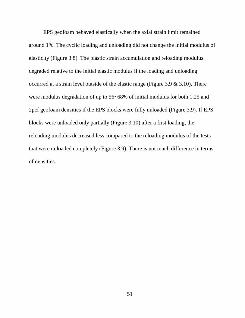
EPS geofoam behaved elastically when the axial strain limit remained
around 1%. The cyclic loading and unloading did not change the initial modulus of
elasticity (Figure 3.8). The plastic strain accumulation and reloading modulus
degraded relative to the initial elastic modulus if the loading and unloading
occurred at a strain level outside of the elastic range (Figure 3.9 & 3.10). There
were modulus degradation of up to 56~68% of initial modulus for both 1.25 and
2pcf geofoam densities if the EPS blocks were fully unloaded (Figure 3.9). If EPS
blocks were unloaded only partially (Figure 3.10) after a first loading, the
reloading modulus decreased less compared to the reloading modulus of the tests
that were unloaded completely (Figure 3.9). There is not much difference in terms
of densities.
51
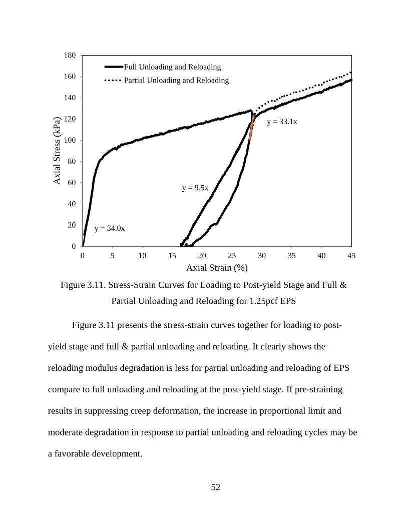
Figure 3.11. Stress-Strain Curves for Loading to Post-yield Stage and Full &
Partial Unloading and Reloading for 1.25pcf EPS
Figure 3.11 presents the stress-strain curves together for loading to post-
yield stage and full & partial unloading and reloading. It clearly shows the
reloading modulus degradation is less for partial unloading and reloading of EPS
compare to full unloading and reloading at the post-yield stage. If pre-straining
results in suppressing creep deformation, the increase in proportional limit and
moderate degradation in response to partial unloading and reloading cycles may be
a favorable development.
y = 34.0x
y = 9.5x
y = 33.1x
0
20
40
60
80
100
120
140
160
180
0 5 10 15 20 25 30 35 40 45
Axi
al S
tress
(kPa
)
Axial Strain (%)
Full Unloading and Reloading
Partial Unloading and Reloading
52
3.3 Conclusions
1. Loading and unloading cycles conducted in the pre-yield stage or near
yield did not produce significant modulus degradation.
2. Loading to post-yield stage and full unloading and reloading cycles
produced significant modulus degradation of up to 56~68% of initial modulus.
3. Loading to post-yield stage and partial unloading and reloading cycles
produced much less modulus degradation than full unloading and reloading cycles.
4. On unloading and reloading, the proportional limit increases with
accumulated strain. The results suggested controlled pre-stressing of geofoam fill
can be beneficial in reducing initial deformations while improving the allowable
working stress range. EPS geofoam tends to develop softer reloading modulus but
continue to strain harden, and stiffen beyond the max load history level.
5. If pre-straining results in suppressing creep deformation, the increase in
proportional limit and moderate degradation in response to partial unloading and
reloading cycles may be a favorable development.
53
CHAPTER 4
STRESS DISTRIBUTION WITHIN EPS BLOCKS BY USING
IMAGE ANALYSIS
Previous laboratory testing of EPS geofoam relied on physical contact and
global deformation monitoring to characterize stress-strain behaviors.
Displacement monitoring in conditions involving submersion in water and
confining pressure or tests in extreme temperature chambers are difficult to
perform with contact detection. ARAMIS is a 3D optical displacement tracking
system for full field or localized non-contact continuous monitoring. A GeoJac
automatic load testing system with a conventional displacement transducer was
used together with ARAMIS. The ARAMIS system consists of two CCD cameras
mounted on a tripod and a track beam. The separation of the cameras and distance
of the tripod can be adjusted to accommodate full field exposure of the test sample.
Displacement and stress-strain results derived from conventional global
measurements were compared with data recorded by the ARAMIS system.
4.1 Background
Determining the deformation response of geofoam under load is important in
developing an in-depth understanding of the engineering behavior. Current strain
determination methods employed as part of compression tests mostly assume that
the strain is uniform throughout the specimen and, hence, are incapable of
54
determining local strains. There is no specified standards for the scattering of the
vertical strains over the height of the EPS specimen. In order to determine the local
deformation and internal strain distribution of EPS specimens, many attempts were
done by previous researchers. The geofoam material was installed with strain
gauges and had occasionally been instrumented with extensometers (Elragi, 2001).
However, these direct contact methods had limitations in fully defining strain
distributions in a test specimen. With the development of technology, a new 3D
optical displacement tracking system for full field or localized continuous
monitoring provide the possibility of developing a more effective way of tracking
deformations without contacting the material.
4.2 ARAMIS System
ARAMIS refers to an optical 3D non-contact deformation measurement
system. Using high resolution digital cameras and advanced techniques of tracking
and distributing the coordinates of pixels, the surface structure of the material is
observed. The observation process starts with calibration of the system with known
distance. Subsequently, segmental images of the test material are determined using
proprietary software. For the materials that do not have surfaces with color or grey
scale contrast, prior application of spray pattern will be necessary. Under live and
dead load conditions, ARAMIS is especially preferable to track dynamic
deformation states as an optical system.
55
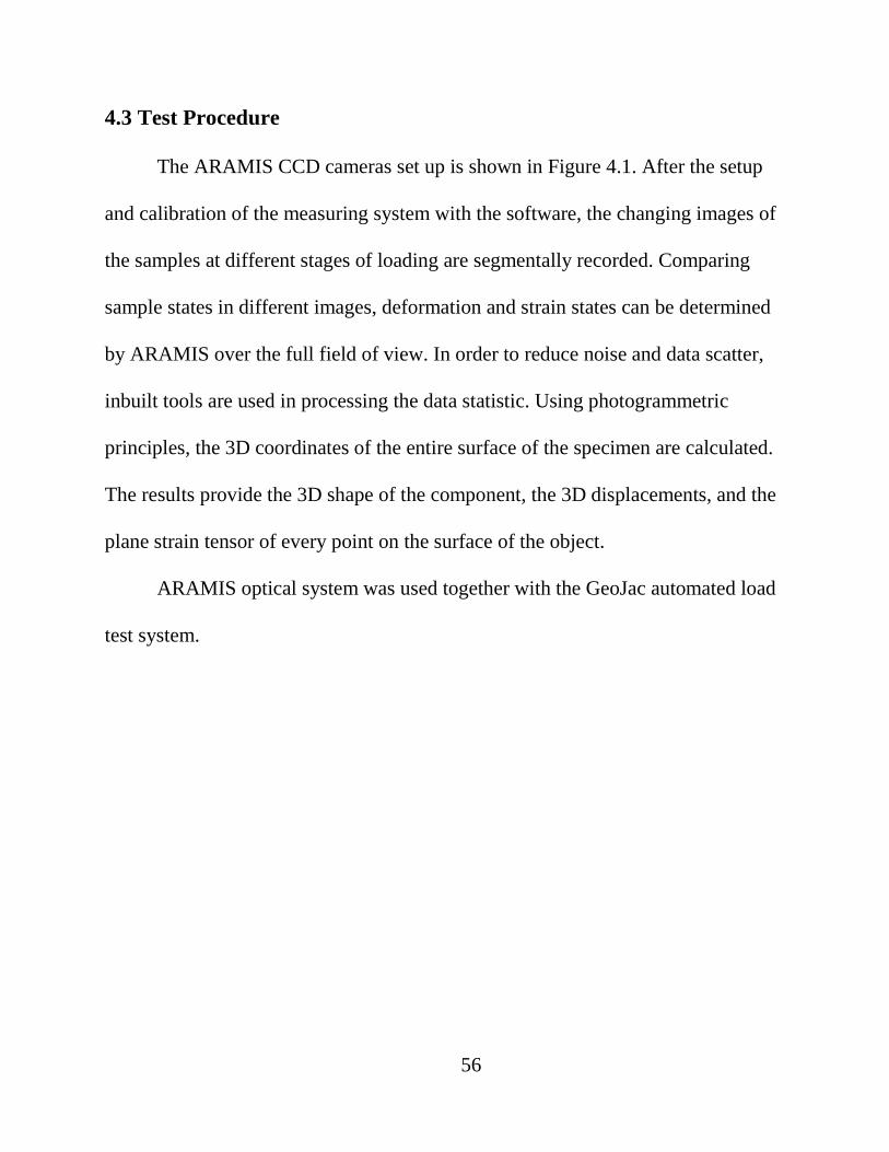
4.3 Test Procedure
The ARAMIS CCD cameras set up is shown in Figure 4.1. After the setup
and calibration of the measuring system with the software, the changing images of
the samples at different stages of loading are segmentally recorded. Comparing
sample states in different images, deformation and strain states can be determined
by ARAMIS over the full field of view. In order to reduce noise and data scatter,
inbuilt tools are used in processing the data statistic. Using photogrammetric
principles, the 3D coordinates of the entire surface of the specimen are calculated.
The results provide the 3D shape of the component, the 3D displacements, and the
plane strain tensor of every point on the surface of the object.
ARAMIS optical system was used together with the GeoJac automated load
test system.
56
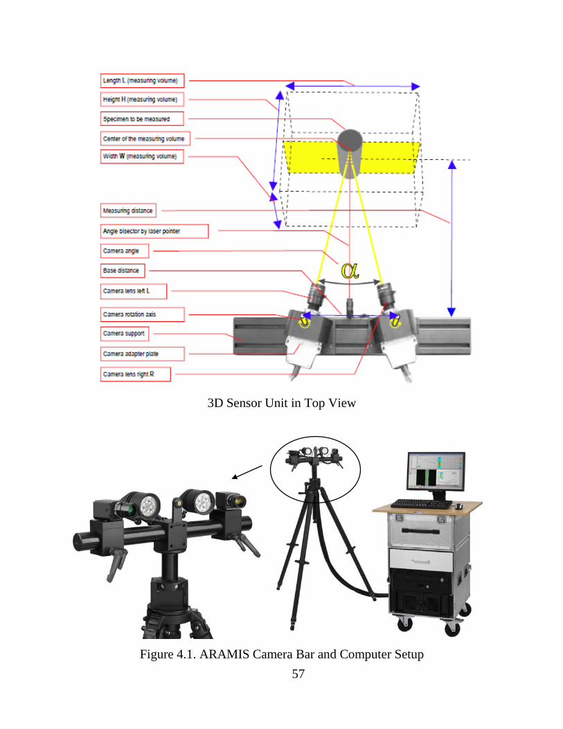
3D Sensor Unit in Top View
Figure 4.1. ARAMIS Camera Bar and Computer Setup
57
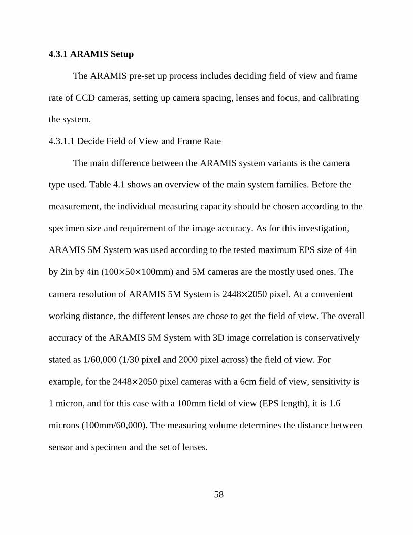
4.3.1 ARAMIS Setup
The ARAMIS pre-set up process includes deciding field of view and frame
rate of CCD cameras, setting up camera spacing, lenses and focus, and calibrating
the system.
4.3.1.1 Decide Field of View and Frame Rate
The main difference between the ARAMIS system variants is the camera
type used. Table 4.1 shows an overview of the main system families. Before the
measurement, the individual measuring capacity should be chosen according to the
specimen size and requirement of the image accuracy. As for this investigation,
ARAMIS 5M System was used according to the tested maximum EPS size of 4in
by 2in by 4in (100×50×100mm) and 5M cameras are the mostly used ones. The
camera resolution of ARAMIS 5M System is 2448×2050 pixel. At a convenient
working distance, the different lenses are chose to get the field of view. The overall
accuracy of the ARAMIS 5M System with 3D image correlation is conservatively
stated as 1/60,000 (1/30 pixel and 2000 pixel across) the field of view. For
example, for the 2448×2050 pixel cameras with a 6cm field of view, sensitivity is
1 micron, and for this case with a 100mm field of view (EPS length), it is 1.6
microns (100mm/60,000). The measuring volume determines the distance between
sensor and specimen and the set of lenses.
58
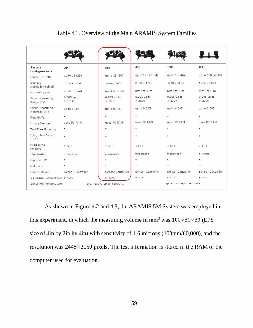
Table 4.1. Overview of the Main ARAMIS System Families
As shown in Figure 4.2 and 4.3, the ARAMIS 5M System was employed in
this experiment, in which the measuring volume in mm3 was 100×80×80 (EPS
size of 4in by 2in by 4in) with sensitivity of 1.6 microns (100mm/60,000), and the
resolution was 2448×2050 pixels. The test information is stored in the RAM of the
computer used for evaluation.
59
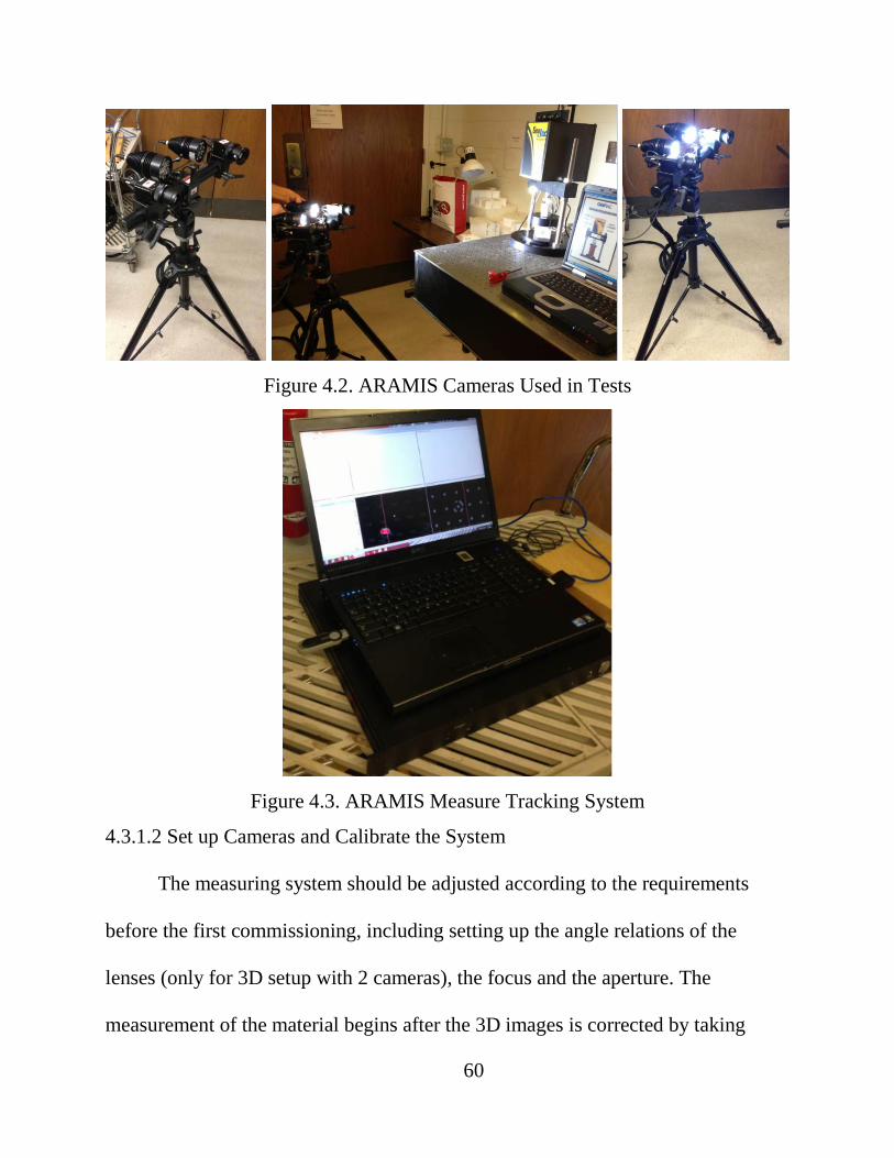
Figure 4.2. ARAMIS Cameras Used in Tests
Figure 4.3. ARAMIS Measure Tracking System
4.3.1.2 Set up Cameras and Calibrate the System
The measuring system should be adjusted according to the requirements
before the first commissioning, including setting up the angle relations of the
lenses (only for 3D setup with 2 cameras), the focus and the aperture. The
measurement of the material begins after the 3D images is corrected by taking
60

calibration readings. The 3D image calibration uses NIST (National Institute of
Standards and Technology) -traceable calibration panels for each field of view. A
sequence of pictures of the panel at different distances and orientations is captured.
Then a photogrammetry process known as bundle adjustment is used to establish
the precise relationship between the two cameras. This is essentially a ray-tracing
process to find unique intersection points, similar to how a GPS system
triangulates coordinates. Each dot on the calibration panel occupies more than 100
pixels on each camera sensor, so dot centers can be interpolated with sub-pixel
accuracy.
For measurements after calibration, the edges of each facet are located based
on local features of the applied pattern. An example final calibration result is
shown in Figure 4.4.
61
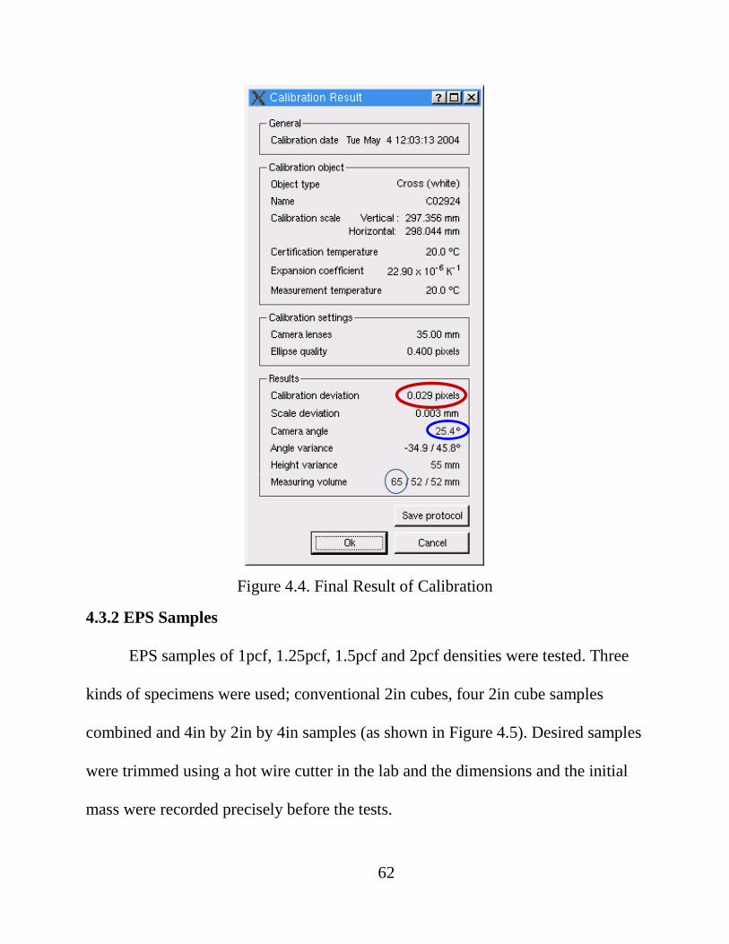
Figure 4.4. Final Result of Calibration
4.3.2 EPS Samples
EPS samples of 1pcf, 1.25pcf, 1.5pcf and 2pcf densities were tested. Three
kinds of specimens were used; conventional 2in cubes, four 2in cube samples
combined and 4in by 2in by 4in samples (as shown in Figure 4.5). Desired samples
were trimmed using a hot wire cutter in the lab and the dimensions and the initial
mass were recorded precisely before the tests.
62

Figure 4.5. Tests Setup
For optical detection of deformation, the material surface structure should be
relatively smooth. There should be a measureable surface pattern so as to clearly
track the target image. Sample preparation consists of applying a regular or random
high contrast dot pattern to the surface, typically with an airbrush. Thousands of
unique correlation areas known as facets (typically up to about 15 pixels in size,
for 5M camera is 19 pixels in size) are defined across the entire imaging area. A
sharp contrast between patterns must exist for the system to work. First of all, the
dimension of the surface traits should be small enough to produce a good raster. 63
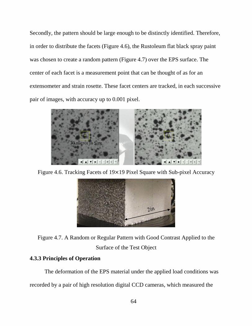
Secondly, the pattern should be large enough to be distinctly identified. Therefore,
in order to distribute the facets (Figure 4.6), the Rustoleum flat black spray paint
was chosen to create a random pattern (Figure 4.7) over the EPS surface. The
center of each facet is a measurement point that can be thought of as for an
extensometer and strain rosette. These facet centers are tracked, in each successive
pair of images, with accuracy up to 0.001 pixel.
Figure 4.6. Tracking Facets of 19×19 Pixel Square with Sub-pixel Accuracy
Figure 4.7. A Random or Regular Pattern with Good Contrast Applied to the
Surface of the Test Object
4.3.3 Principles of Operation
The deformation of the EPS material under the applied load conditions was
recorded by a pair of high resolution digital CCD cameras, which measured the
30 micros in Size
64

sample’s 3D coordinates and the 3D deformations. The initial image processing
defines unique correlation areas known as macro-image facets, typically 5-20
pixels square, across the entire imaging area. Each facet center was a measurement
point.
The key to 3D Image Correlation is that it tracks changes in an applied
micro-pattern (random pattern), rather than a projected pattern, using ordinary
white light. The system tracks this random pattern applied to the measurement
surface with sub-pixel accuracy. This means that as long as the object remains
within the field of view of the cameras, all of the local deformations can be tracked.
Then the strain can be derived once the deformations are tracked. Thus, large
deformations can be analyzed in a single measurement.
As shown in the Figure 4.2, the camera pair was simply placed in front of
the test sample at the calibrated working distance. The recorded results from
ARAMIS system are the 3D shape of the component, the 3D displacements, and
the derived strains. 3D coordinates of each facet determined for each picture set
was recorded by the software. 3D coordinates can be synchronized to 2D by using
photogrammetry technology.
65

(a) Object 3D Coordinate System (b) Image 2D Coordinate System
(c) Rotation Parameters
Figure 4.8. Coordinate Systems of Transferring 3D Coordinate to 2D
The mapping function for transferring 3D coordinates (Figure 4.8 (a)) to 2D
(Figure 4.8 (b)) can be expressed as shown in Equation 4.1 and 4.2.
𝜉𝜉 = 𝜉𝜉0 − 𝑐𝑐𝑘𝑘𝑟𝑟11(𝑋𝑋−𝑋𝑋0)+𝑟𝑟12(𝑌𝑌−𝑌𝑌0)+𝑟𝑟13(𝑍𝑍−𝑍𝑍0)𝑟𝑟31(𝑋𝑋−𝑋𝑋0)+𝑟𝑟32(𝑌𝑌−𝑌𝑌0)+𝑟𝑟33(𝑍𝑍−𝑍𝑍0)
…………….. Equation 4.1
𝜂𝜂 = 𝜂𝜂0 − 𝑐𝑐𝑘𝑘𝑟𝑟21(𝑋𝑋−𝑋𝑋0)+𝑟𝑟22(𝑌𝑌−𝑌𝑌0)+𝑟𝑟32(𝑍𝑍−𝑍𝑍0)𝑟𝑟31(𝑋𝑋−𝑋𝑋0)+𝑟𝑟32(𝑌𝑌−𝑌𝑌0)+𝑟𝑟33(𝑍𝑍−𝑍𝑍0)
…………….. Equation 4.2
Where,
𝜉𝜉, 𝜂𝜂 = Measured Point coordinates of the 2D image;
𝜉𝜉0, 𝜂𝜂0 = Principle Point coordinates of the 2D image;
O´
66
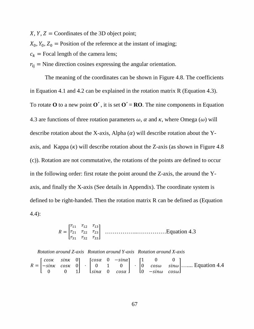
𝑋𝑋, 𝑌𝑌, 𝑍𝑍 = Coordinates of the 3D object point;
𝑋𝑋0, 𝑌𝑌0, 𝑍𝑍0 = Position of the reference at the instant of imaging;
𝑐𝑐𝑘𝑘 = Focal length of the camera lens;
𝑟𝑟ij = Nine direction cosines expressing the angular orientation.
The meaning of the coordinates can be shown in Figure 4.8. The coefficients
in Equation 4.1 and 4.2 can be explained in the rotation matrix R (Equation 4.3).
To rotate O to a new point O´, it is set O´= RO. The nine components in Equation
4.3 are functions of three rotation parameters 𝜔𝜔, 𝛼𝛼 and 𝜅𝜅, where Omega (𝜔𝜔) will
describe rotation about the X-axis, Alpha (𝛼𝛼) will describe rotation about the Y-
axis, and Kappa (𝜅𝜅) will describe rotation about the Z-axis (as shown in Figure 4.8
(c)). Rotation are not commutative, the rotations of the points are defined to occur
in the following order: first rotate the point around the Z-axis, the around the Y-
axis, and finally the X-axis (See details in Appendix). The coordinate system is
defined to be right-handed. Then the rotation matrix R can be defined as (Equation
4.4):
𝑅𝑅 = �𝑟𝑟11 𝑟𝑟12 𝑟𝑟13𝑟𝑟21 𝑟𝑟22 𝑟𝑟23𝑟𝑟31 𝑟𝑟32 𝑟𝑟33
� ……………..……………Equation 4.3
Rotation around Z-axis Rotation around Y-axis Rotation around X-axis
𝑅𝑅 = �𝑐𝑐𝑐𝑐𝑐𝑐𝜅𝜅 𝑐𝑐𝑖𝑖𝑠𝑠𝜅𝜅 0−𝑐𝑐𝑖𝑖𝑠𝑠𝜅𝜅 𝑐𝑐𝑐𝑐𝑐𝑐𝜅𝜅 0
0 0 1� · �
𝑐𝑐𝑐𝑐𝑐𝑐𝛼𝛼 0 −𝑐𝑐𝑖𝑖𝑠𝑠𝛼𝛼0 1 0
𝑐𝑐𝑖𝑖𝑠𝑠𝛼𝛼 0 𝑐𝑐𝑐𝑐𝑐𝑐𝛼𝛼� · �
1 0 00 𝑐𝑐𝑐𝑐𝑐𝑐𝜔𝜔 𝑐𝑐𝑖𝑖𝑠𝑠𝜔𝜔0 −𝑐𝑐𝑖𝑖𝑠𝑠𝜔𝜔 𝑐𝑐𝑐𝑐𝑐𝑐𝜔𝜔
�….... Equation 4.4
67
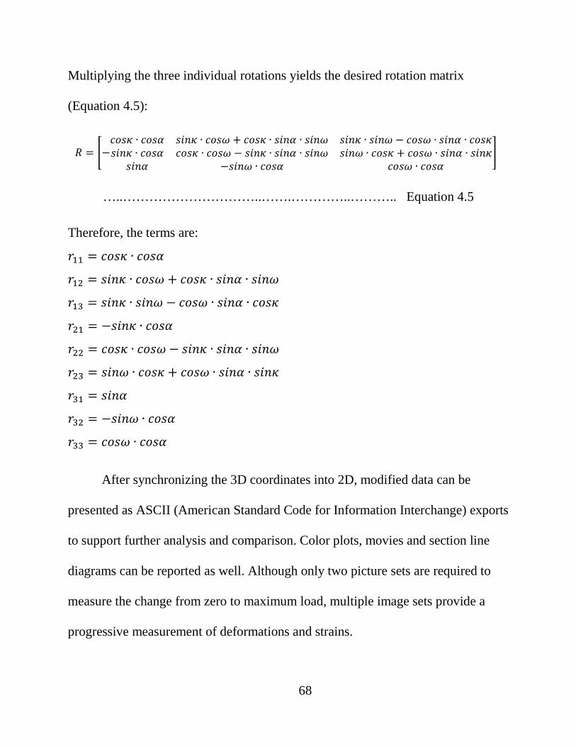
Multiplying the three individual rotations yields the desired rotation matrix
(Equation 4.5):
𝑅𝑅 = �−𝑐𝑐𝑐𝑐𝑐𝑐𝜅𝜅 ∙ 𝑐𝑐𝑐𝑐𝑐𝑐𝛼𝛼 𝑐𝑐𝑖𝑖𝑠𝑠𝜅𝜅 ∙ 𝑐𝑐𝑐𝑐𝑐𝑐𝜔𝜔 + 𝑐𝑐𝑐𝑐𝑐𝑐𝜅𝜅 ∙ 𝑐𝑐𝑖𝑖𝑠𝑠𝛼𝛼 ∙ 𝑐𝑐𝑖𝑖𝑠𝑠𝜔𝜔 𝑐𝑐𝑖𝑖𝑠𝑠𝜅𝜅 ∙ 𝑐𝑐𝑖𝑖𝑠𝑠𝜔𝜔 − 𝑐𝑐𝑐𝑐𝑐𝑐𝜔𝜔 ∙ 𝑐𝑐𝑖𝑖𝑠𝑠𝛼𝛼 ∙ 𝑐𝑐𝑐𝑐𝑐𝑐𝜅𝜅𝑐𝑐𝑖𝑖𝑠𝑠𝜅𝜅 ∙ 𝑐𝑐𝑐𝑐𝑐𝑐𝛼𝛼 𝑐𝑐𝑐𝑐𝑐𝑐𝜅𝜅 ∙ 𝑐𝑐𝑐𝑐𝑐𝑐𝜔𝜔 − 𝑐𝑐𝑖𝑖𝑠𝑠𝜅𝜅 ∙ 𝑐𝑐𝑖𝑖𝑠𝑠𝛼𝛼 ∙ 𝑐𝑐𝑖𝑖𝑠𝑠𝜔𝜔 𝑐𝑐𝑖𝑖𝑠𝑠𝜔𝜔 ∙ 𝑐𝑐𝑐𝑐𝑐𝑐𝜅𝜅 + 𝑐𝑐𝑐𝑐𝑐𝑐𝜔𝜔 ∙ 𝑐𝑐𝑖𝑖𝑠𝑠𝛼𝛼 ∙ 𝑐𝑐𝑖𝑖𝑠𝑠𝜅𝜅
𝑐𝑐𝑖𝑖𝑠𝑠𝛼𝛼 −𝑐𝑐𝑖𝑖𝑠𝑠𝜔𝜔 ∙ 𝑐𝑐𝑐𝑐𝑐𝑐𝛼𝛼 𝑐𝑐𝑐𝑐𝑐𝑐𝜔𝜔 ∙ 𝑐𝑐𝑐𝑐𝑐𝑐𝛼𝛼�
…..…………………………..…….…………..……….. Equation 4.5
Therefore, the terms are:
𝑟𝑟11 = 𝑐𝑐𝑐𝑐𝑐𝑐𝜅𝜅 ∙ 𝑐𝑐𝑐𝑐𝑐𝑐𝛼𝛼
𝑟𝑟12 = 𝑐𝑐𝑖𝑖𝑠𝑠𝜅𝜅 ∙ 𝑐𝑐𝑐𝑐𝑐𝑐𝜔𝜔 + 𝑐𝑐𝑐𝑐𝑐𝑐𝜅𝜅 ∙ 𝑐𝑐𝑖𝑖𝑠𝑠𝛼𝛼 ∙ 𝑐𝑐𝑖𝑖𝑠𝑠𝜔𝜔
𝑟𝑟13 = 𝑐𝑐𝑖𝑖𝑠𝑠𝜅𝜅 ∙ 𝑐𝑐𝑖𝑖𝑠𝑠𝜔𝜔 − 𝑐𝑐𝑐𝑐𝑐𝑐𝜔𝜔 ∙ 𝑐𝑐𝑖𝑖𝑠𝑠𝛼𝛼 ∙ 𝑐𝑐𝑐𝑐𝑐𝑐𝜅𝜅
𝑟𝑟21 = −𝑐𝑐𝑖𝑖𝑠𝑠𝜅𝜅 ∙ 𝑐𝑐𝑐𝑐𝑐𝑐𝛼𝛼
𝑟𝑟22 = 𝑐𝑐𝑐𝑐𝑐𝑐𝜅𝜅 ∙ 𝑐𝑐𝑐𝑐𝑐𝑐𝜔𝜔 − 𝑐𝑐𝑖𝑖𝑠𝑠𝜅𝜅 ∙ 𝑐𝑐𝑖𝑖𝑠𝑠𝛼𝛼 ∙ 𝑐𝑐𝑖𝑖𝑠𝑠𝜔𝜔
𝑟𝑟23 = 𝑐𝑐𝑖𝑖𝑠𝑠𝜔𝜔 ∙ 𝑐𝑐𝑐𝑐𝑐𝑐𝜅𝜅 + 𝑐𝑐𝑐𝑐𝑐𝑐𝜔𝜔 ∙ 𝑐𝑐𝑖𝑖𝑠𝑠𝛼𝛼 ∙ 𝑐𝑐𝑖𝑖𝑠𝑠𝜅𝜅
𝑟𝑟31 = 𝑐𝑐𝑖𝑖𝑠𝑠𝛼𝛼
𝑟𝑟32 = −𝑐𝑐𝑖𝑖𝑠𝑠𝜔𝜔 ∙ 𝑐𝑐𝑐𝑐𝑐𝑐𝛼𝛼
𝑟𝑟33 = 𝑐𝑐𝑐𝑐𝑐𝑐𝜔𝜔 ∙ 𝑐𝑐𝑐𝑐𝑐𝑐𝛼𝛼
After synchronizing the 3D coordinates into 2D, modified data can be
presented as ASCII (American Standard Code for Information Interchange) exports
to support further analysis and comparison. Color plots, movies and section line
diagrams can be reported as well. Although only two picture sets are required to
measure the change from zero to maximum load, multiple image sets provide a
progressive measurement of deformations and strains.
68
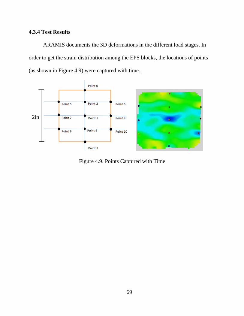
4.3.4 Test Results
ARAMIS documents the 3D deformations in the different load stages. In
order to get the strain distribution among the EPS blocks, the locations of points
(as shown in Figure 4.9) were captured with time.
Figure 4.9. Points Captured with Time
2in
69
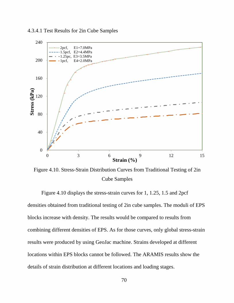
4.3.4.1 Test Results for 2in Cube Samples
Figure 4.10. Stress-Strain Distribution Curves from Traditional Testing of 2in
Cube Samples
Figure 4.10 displays the stress-strain curves for 1, 1.25, 1.5 and 2pcf
densities obtained from traditional testing of 2in cube samples. The moduli of EPS
blocks increase with density. The results would be compared to results from
combining different densities of EPS. As for those curves, only global stress-strain
results were produced by using GeoJac machine. Strains developed at different
locations within EPS blocks cannot be followed. The ARAMIS results show the
details of strain distribution at different locations and loading stages.
0
40
80
120
160
200
240
0 3 6 9 12 15
Stre
ss (k
Pa)
Strain (%)
2pcf, E1=7.0MPa1.5pcf, E2=4.4MPa1.25pc, E3=3.5MPa1pcf, E4=2.0MPa
70

Figure 4.11 (a) Strain Derived from Displacement
71
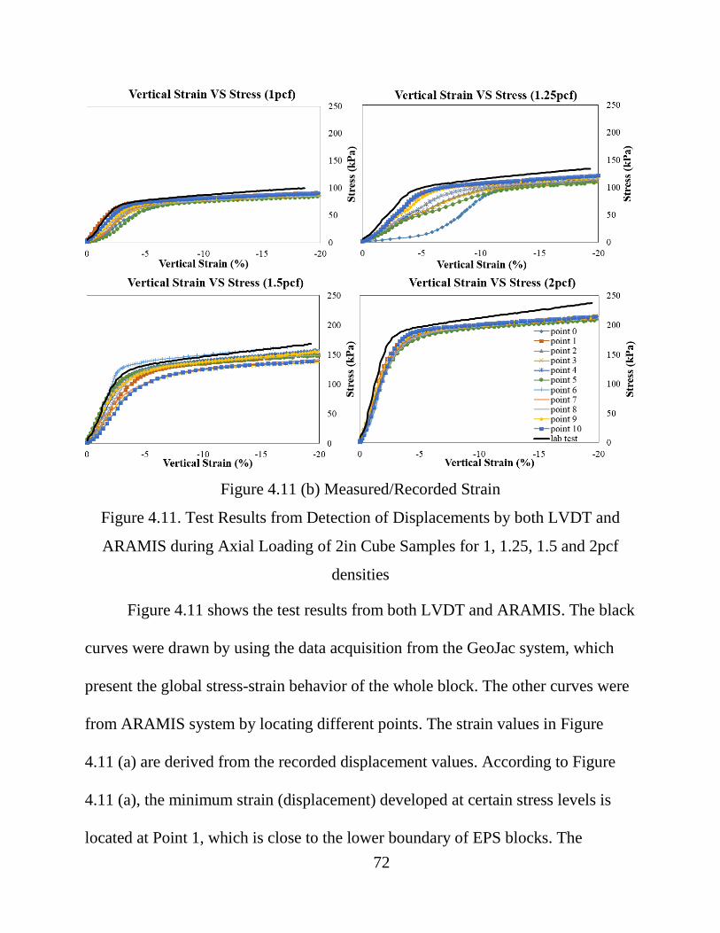
Figure 4.11 (b) Measured/Recorded Strain
Figure 4.11. Test Results from Detection of Displacements by both LVDT and
ARAMIS during Axial Loading of 2in Cube Samples for 1, 1.25, 1.5 and 2pcf
densities
Figure 4.11 shows the test results from both LVDT and ARAMIS. The black
curves were drawn by using the data acquisition from the GeoJac system, which
present the global stress-strain behavior of the whole block. The other curves were
from ARAMIS system by locating different points. The strain values in Figure
4.11 (a) are derived from the recorded displacement values. According to Figure
4.11 (a), the minimum strain (displacement) developed at certain stress levels is
located at Point 1, which is close to the lower boundary of EPS blocks. The 72
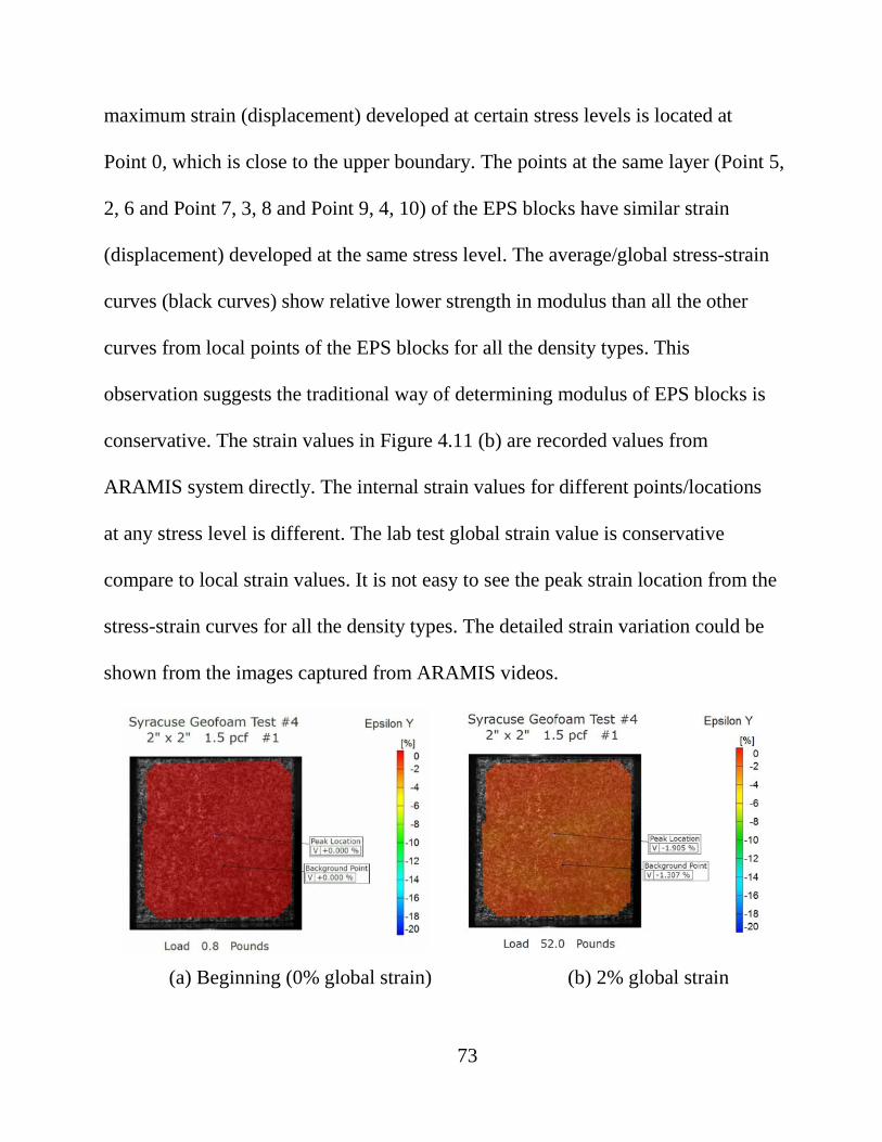
maximum strain (displacement) developed at certain stress levels is located at
Point 0, which is close to the upper boundary. The points at the same layer (Point 5,
2, 6 and Point 7, 3, 8 and Point 9, 4, 10) of the EPS blocks have similar strain
(displacement) developed at the same stress level. The average/global stress-strain
curves (black curves) show relative lower strength in modulus than all the other
curves from local points of the EPS blocks for all the density types. This
observation suggests the traditional way of determining modulus of EPS blocks is
conservative. The strain values in Figure 4.11 (b) are recorded values from
ARAMIS system directly. The internal strain values for different points/locations
at any stress level is different. The lab test global strain value is conservative
compare to local strain values. It is not easy to see the peak strain location from the
stress-strain curves for all the density types. The detailed strain variation could be
shown from the images captured from ARAMIS videos.
(a) Beginning (0% global strain) (b) 2% global strain
73
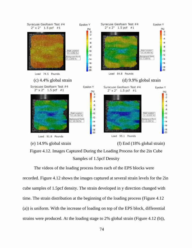
(c) 4.4% global strain (d) 9.9% global strain
(e) 14.9% global strain (f) End (18% global strain)
Figure 4.12. Images Captured During the Loading Process for the 2in Cube
Samples of 1.5pcf Density
The videos of the loading process from each of the EPS blocks were
recorded. Figure 4.12 shows the images captured at several strain levels for the 2in
cube samples of 1.5pcf density. The strain developed in y direction changed with
time. The strain distribution at the beginning of the loading process (Figure 4.12
(a)) is uniform. With the increase of loading on top of the EPS block, differential
strains were produced. At the loading stage to 2% global strain (Figure 4.12 (b)),
74
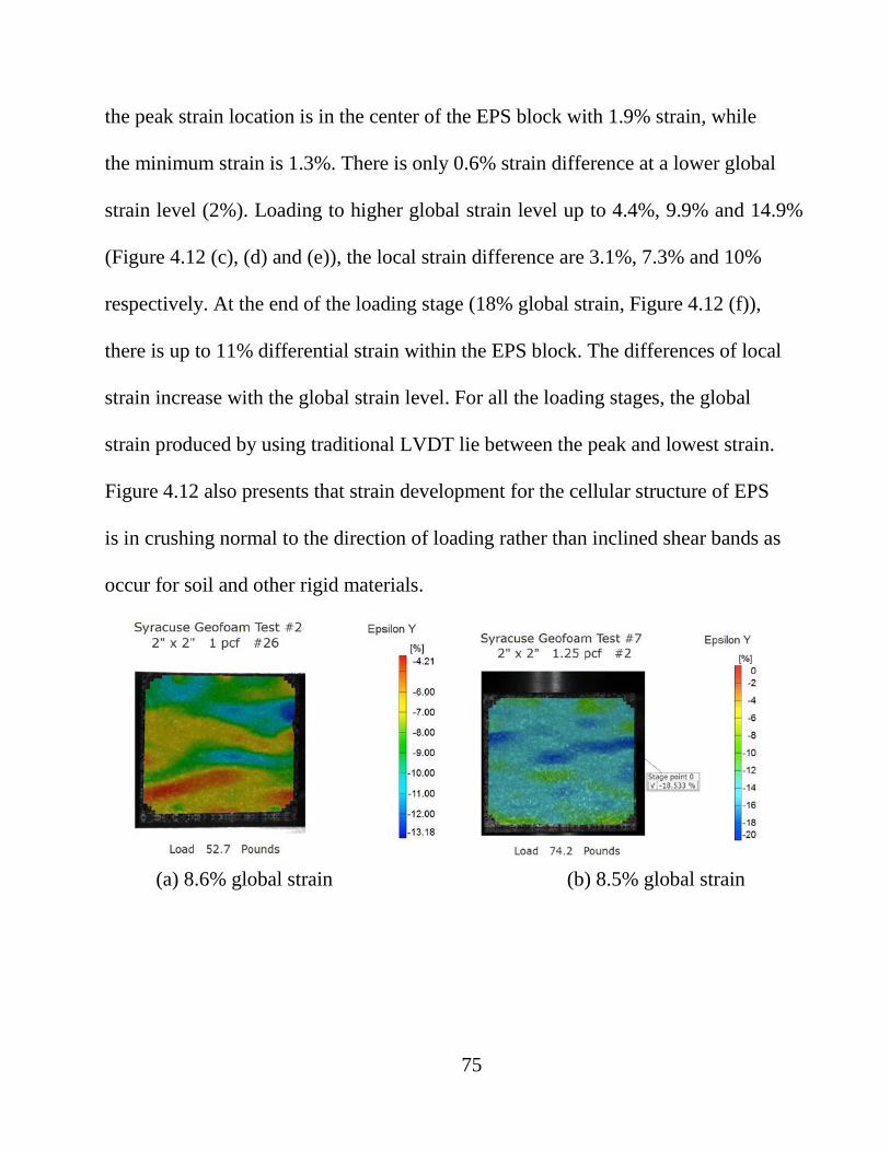
the peak strain location is in the center of the EPS block with 1.9% strain, while
the minimum strain is 1.3%. There is only 0.6% strain difference at a lower global
strain level (2%). Loading to higher global strain level up to 4.4%, 9.9% and 14.9%
(Figure 4.12 (c), (d) and (e)), the local strain difference are 3.1%, 7.3% and 10%
respectively. At the end of the loading stage (18% global strain, Figure 4.12 (f)),
there is up to 11% differential strain within the EPS block. The differences of local
strain increase with the global strain level. For all the loading stages, the global
strain produced by using traditional LVDT lie between the peak and lowest strain.
Figure 4.12 also presents that strain development for the cellular structure of EPS
is in crushing normal to the direction of loading rather than inclined shear bands as
occur for soil and other rigid materials.
(a) 8.6% global strain (b) 8.5% global strain
75
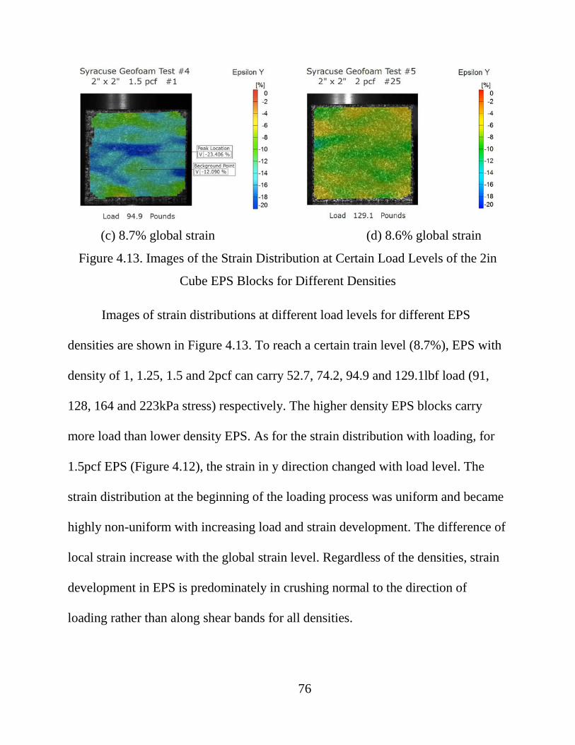
(c) 8.7% global strain (d) 8.6% global strain
Figure 4.13. Images of the Strain Distribution at Certain Load Levels of the 2in
Cube EPS Blocks for Different Densities
Images of strain distributions at different load levels for different EPS
densities are shown in Figure 4.13. To reach a certain train level (8.7%), EPS with
density of 1, 1.25, 1.5 and 2pcf can carry 52.7, 74.2, 94.9 and 129.1lbf load (91,
128, 164 and 223kPa stress) respectively. The higher density EPS blocks carry
more load than lower density EPS. As for the strain distribution with loading, for
1.5pcf EPS (Figure 4.12), the strain in y direction changed with load level. The
strain distribution at the beginning of the loading process was uniform and became
highly non-uniform with increasing load and strain development. The difference of
local strain increase with the global strain level. Regardless of the densities, strain
development in EPS is predominately in crushing normal to the direction of
loading rather than along shear bands for all densities.
76
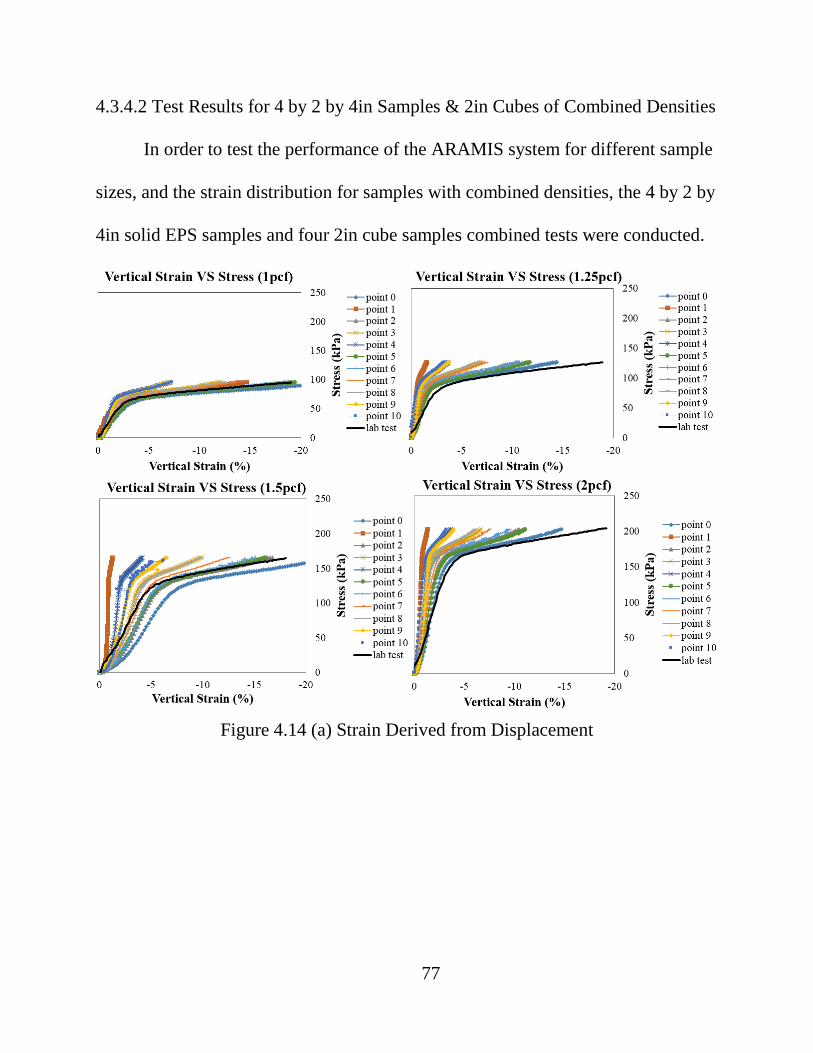
4.3.4.2 Test Results for 4 by 2 by 4in Samples & 2in Cubes of Combined Densities
In order to test the performance of the ARAMIS system for different sample
sizes, and the strain distribution for samples with combined densities, the 4 by 2 by
4in solid EPS samples and four 2in cube samples combined tests were conducted.
Figure 4.14 (a) Strain Derived from Displacement
77
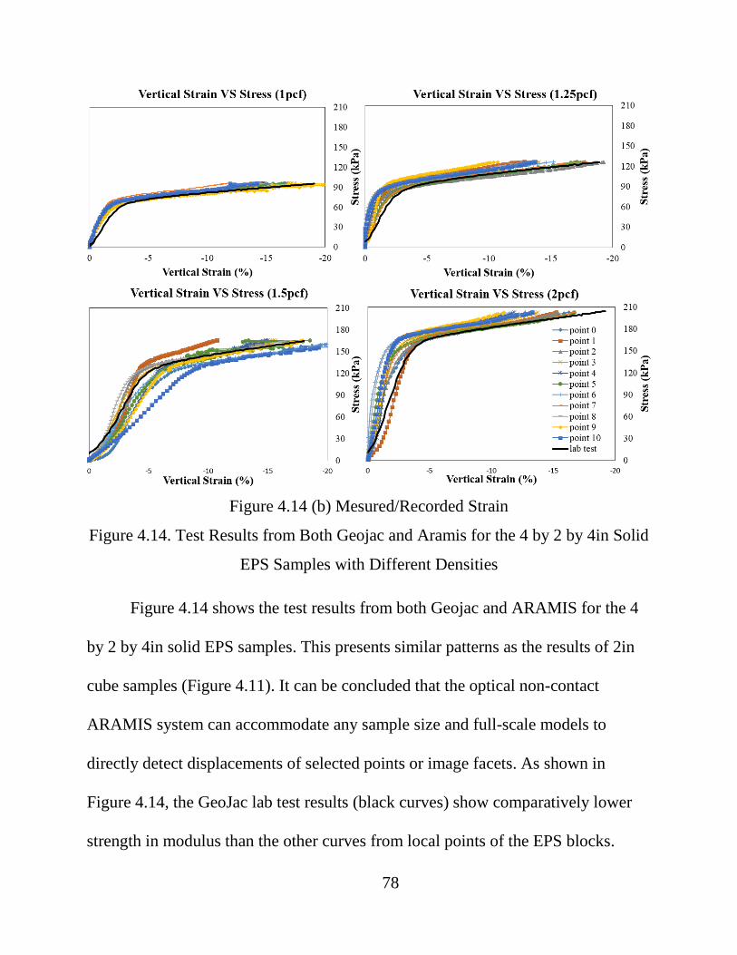
Figure 4.14 (b) Mesured/Recorded Strain
Figure 4.14. Test Results from Both Geojac and Aramis for the 4 by 2 by 4in Solid
EPS Samples with Different Densities
Figure 4.14 shows the test results from both Geojac and ARAMIS for the 4
by 2 by 4in solid EPS samples. This presents similar patterns as the results of 2in
cube samples (Figure 4.11). It can be concluded that the optical non-contact
ARAMIS system can accommodate any sample size and full-scale models to
directly detect displacements of selected points or image facets. As shown in
Figure 4.14, the GeoJac lab test results (black curves) show comparatively lower
strength in modulus than the other curves from local points of the EPS blocks.
78
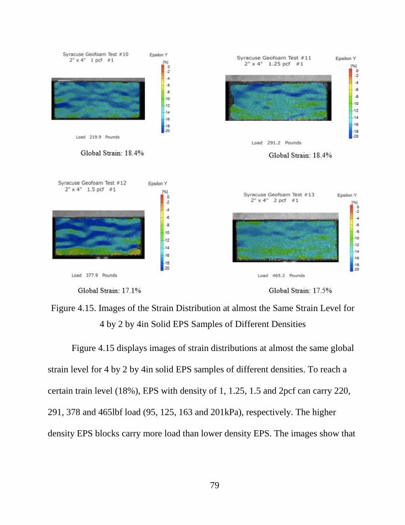
Figure 4.15. Images of the Strain Distribution at almost the Same Strain Level for
4 by 2 by 4in Solid EPS Samples of Different Densities
Figure 4.15 displays images of strain distributions at almost the same global
strain level for 4 by 2 by 4in solid EPS samples of different densities. To reach a
certain train level (18%), EPS with density of 1, 1.25, 1.5 and 2pcf can carry 220,
291, 378 and 465lbf load (95, 125, 163 and 201kPa), respectively. The higher
density EPS blocks carry more load than lower density EPS. The images show that
79

the strain distribution are not uniform and the strain development for the EPS
structure are in crushing normal to the direction of loading.
(a) Beginning (b) End
Figure 4.16. Images Captured at the Beginning and End of the Loading Process for
the 4in by 2in by 4in Samples with Combined 1 & 2pcf Densities
Images captured at the beginning and end of the loading process for the 4in
by 2in by 4in samples with combined 1 & 2pcf densities EPS are shown in Figure
4.16. For this test, the boundary displacement conditions were controlled because
of the rigid loading plate. It is difficult to show the strain distribution at the top and
lower boundary because of the rigid boundary. With mixed EPS densities at a load
level of 432lbf (Figure 4.16 (b), the left 2in cube block, which was with 1pcf
density, had around 12% differential strain. While the right 2 in cube block with
density of 2pcf had 20% differential strain. This indicates the dense (2pcf) had
more differential strain distribution compared to the weak (1pcf) EPS sample.
According to the stress-strain behavior of EPS geofoam, the EPS block with higher
2pcf EPS 1pcf EPS 2pcf EPS 1pcf EPS
80
density carried more load compared to the lower density EPS at the same strain
level. In order to further study the load bearing behavior of mixed density
combination, more tests with flexible boundary were performed as presented in
next chapter.
4.4 Conclusions
1. The optical non-contact system can accommodate any sample size and
full-scale models to directly detect displacements of selected points or image facets
at high resolution and in 3D.
2. Synchronizing force sensing with displacement detection, directional
moduli and Poisson’s Ratios can be determined from one test sample.
3. It was verified that the traditional way of determining modulus of EPS
blocks is conservative.
4. The strain distribution across the face of an EPS sample is initially
uniform and becomes highly non-uniform with increasing load and strain
development. The difference of local strain are small at lower global strain level
and high at higher global strain level. For mixed density tests, the dense (2pcf) EPS
blocks were carrying more loads. As a result, the strain level was in between the
higher level for 1pcf and lower level for 2pcf.
5. Time lapse images and video recordings show progressive strain
development for the cellular structure of EPS is in crushing normal to the direction
81

of loading rather than inclined shear bands as occur for soil and other rigid
materials.
82
CHAPTER 5
EFFECTS OF COMBINING DIFFERENT DENSITIES
AND LOCATION OF THE EPS BLOCKS
5.1 Background
The construction process of geofoam material can be varied. The
performance of geofoam can be affected by factors such as the quality control and
density of the EPS blocks. Sometimes, EPS blocks are placed with mixed densities
due to the poor quality control. Experienced constructors place EPS blocks in
layers of uniform density and with staggered vertical joints. But there was no
previous research or lab tests to validate such guidance.
To investigate the importance of quality assurance and proper installation of
EPS geofoam blocks, lab tests with and without different densities and also with
and without vertical continuous joints were performed. Lab tests were also
simulated in FLAC (Finite Difference Model).
5.2 Lab Test Setup
As shown in Figure 5.1, by using the GeoJac loading frame, the samples can
be perpendicularly loaded without confining stress in accordance with ASTM D
1621. The load cell that is suspended from the crossbar of the loading frame
detects the applied vertical force. The vertical displacement is registered by the
displacement transducer (LVDT). 83

Figure 5.1. GeoJac System Setup
A camera on a tripod was set up in front of the test samples to continually
record the loading process. After the test setup, the images were recorded for
different loading stages. Then the deformation of EPS blocks and loading stages
were observed and compared with the position of EPS blocks before loading.
5.3 Lab Test Process
Experiments were conducted on five or six EPS blocks in 2 layers with
either uniform or mixed densities.
(1) In the first test series, six 2in cube samples were stacked in two layers of
three blocks with continuous vertical joints. Three tests were done by using the six
84
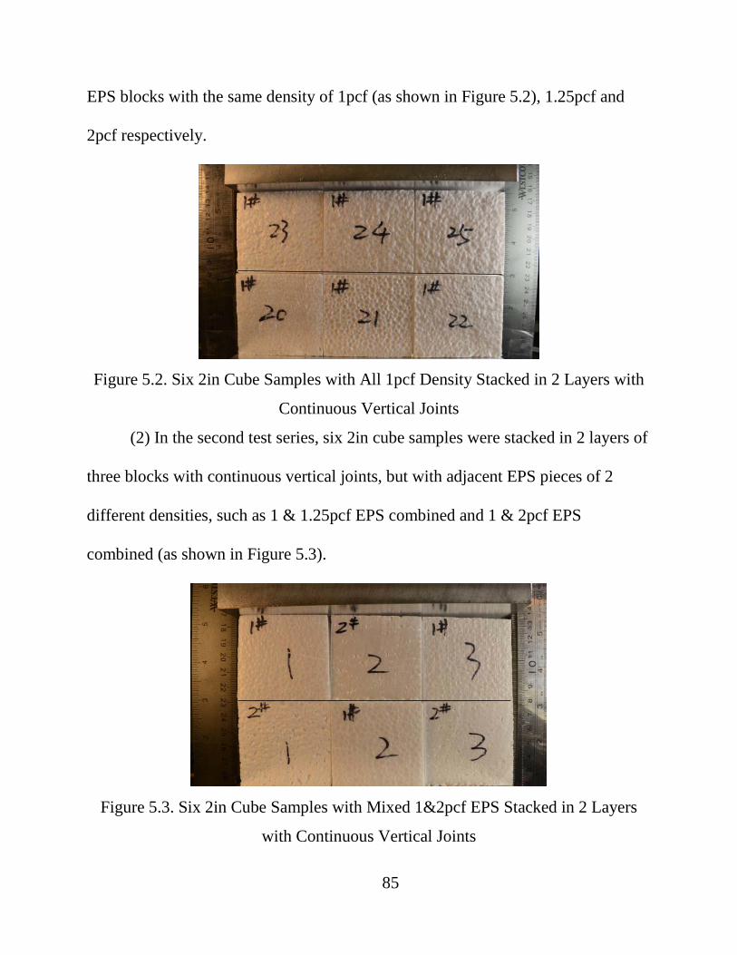
EPS blocks with the same density of 1pcf (as shown in Figure 5.2), 1.25pcf and
2pcf respectively.
Figure 5.2. Six 2in Cube Samples with All 1pcf Density Stacked in 2 Layers with
Continuous Vertical Joints
(2) In the second test series, six 2in cube samples were stacked in 2 layers of
three blocks with continuous vertical joints, but with adjacent EPS pieces of 2
different densities, such as 1 & 1.25pcf EPS combined and 1 & 2pcf EPS
combined (as shown in Figure 5.3).
Figure 5.3. Six 2in Cube Samples with Mixed 1&2pcf EPS Stacked in 2 Layers
with Continuous Vertical Joints
85

(3) In the third test series, five samples were stacked in two layers, replacing
the three 2in cube samples on the top layers with two 3in wide blocks. For these
tests with two upper and three lower blocks, the vertical joints were staggered and
no continuous vertical joints existed across the two layers. Three tests were done
by using the five EPS blocks with the same density of 1pcf (as shown in Figure
5.4), 1.25pcf and 2pcf, respectively.
Figure 5.4. Five EPS Blocks with All 1pcf Density Stacked in 2 Layers without
Continuous Vertical Joints
(4) The fourth test series was the same as the third but with mixed lower and
higher density EPS pieces in the top and lower layers of 1 & 1.25pcf EPS, and 1 &
2pcf EPS combinations (as shown in Figure 5.5). One test was made with three
higher density EPS and two lower density EPS (Figure 5.5), while another was
with three lower density EPS and two higher density EPS.
86

Figure 5.5. Five EPS Blocks with Mixed 1&2pcf EPS Stacked in 2 Layers without
Continuous Vertical Joints
5.4 Test Results
According to the images captured before and after tests (Figure 5.6), samples
deformed equally when the densities were the same. The interface between the
upper and lower blocks remained horizontal, for both cases with and without
continuous vertical joints (6 and 5 EPS samples).
Before Loading After Loading
Figure 5.6 (a). Six 2in Cube Samples with Uniform Density Stacked in 2 Layers
with Continuous Vertical Joints
87

Before Loading After Loading
Figure 5.6 (b). Five 2in Cube Samples with Uniform Density Stacked in 2 Layers
without Continuous Vertical Joints
Figure 5.6. EPS Blocks with All 1pcf Density
In the mixed density tests, the lower density blocks deformed more than the
higher density blocks. The initially horizontal interface between the layers became
uneven (Figure 5.7) for both cases with and without continuous vertical joints. The
unevenness of the interface between the upper and lower blocks was less for the
tests containing five blocks without continuous joints (Figure 5.7 (b) and (c))
compared to the tests using six EPS blocks with continuous vertical joints (Figure
5.7 (a)).
88
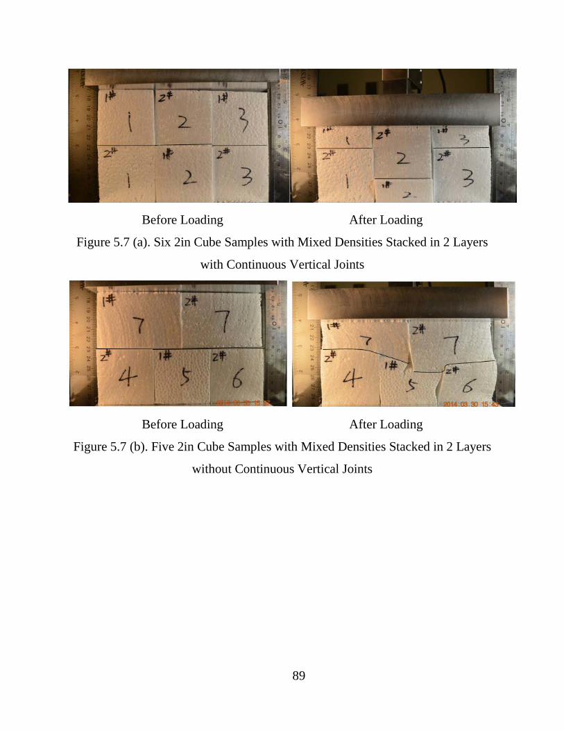
Before Loading After Loading
Figure 5.7 (a). Six 2in Cube Samples with Mixed Densities Stacked in 2 Layers
with Continuous Vertical Joints
Before Loading After Loading
Figure 5.7 (b). Five 2in Cube Samples with Mixed Densities Stacked in 2 Layers
without Continuous Vertical Joints
89
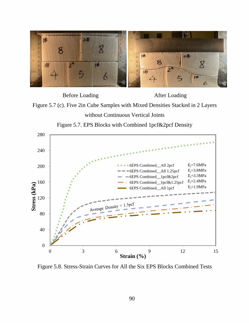
Before Loading After Loading
Figure 5.7 (c). Five 2in Cube Samples with Mixed Densities Stacked in 2 Layers
without Continuous Vertical Joints
Figure 5.7. EPS Blocks with Combined 1pcf&2pcf Density
Figure 5.8. Stress-Strain Curves for All the Six EPS Blocks Combined Tests
0
40
80
120
160
200
240
280
0 3 6 9 12 15
Stre
ss (k
Pa)
Strain (%)
6EPS Combined__All 2pcf6EPS Combined__All 1.25pcf6EPS Combined__1pcf&2pcf6EPS Combined__1pcf&1.25pcf6EPS Combined__All 1pcf Ei=1.9MPa
Ei=7.6MPa
Ei=3.3MPaEi=3.8MPa
Ei=2.4MPa
90
Figure 5.8 shows the stress-strain curves for six EPS blocks of the same and
combined densities. The results indicate EPS blocks with mixed densities had
initial modulus in between the modulus values for the same lower and upper
densities. The strengths at 1, 5 and 10 percent strain for the uniform upper density
set were higher than the corresponding strengths for the mixed density set. The
mixed lower density EPS samples reduced the strength of the higher density EPS
samples. The modulus of the combined density blocks were higher than the
modulus of the lower density EPS. However, a uniform 1.25pcf density set had
higher modulus and strength than a combination of 1 and 2pcf densities; even
though the average densities is 1.5pcf and greater than the uniform set of 1.25pcf
in Figure 5.8.
91

Figure 5.9. Stress-Strain Curves for All the Five EPS Blocks Combined Tests
Figure 5.9 displays the stress-strain curves for five EPS blocks. The general
tendency showed a similar pattern as the six EPS blocks combined tests. The
results demonstrate the initial modulus of EPS blocks with mixed densities are
intermediate between the initial modulus of lower and upper densities. The mixed
lower density EPS samples reduced the strength of the higher density EPS. The
strengths at 1, 5 and 10 percent strain for the uniform upper density set were higher
than the corresponding strengths for the mixed density set. The modulus of the
combined density blocks were higher than the modulus of the lower density EPS.
0
40
80
120
160
200
240
280
0 3 6 9 12 15
Stre
ss (k
Pa)
Strain (%)
5EPS Combined__All 2pcf5EPS Combined__1pcf(2)&2pcf(3)5EPS Combined2__1pcf(3)&2pcf(2)5EPS Combined__All 1.25pcf5EPS Combined__1pcf(2)&1.25pcf(3)5EPS Combined2__1pcf(3)&1.25pcf(2)5EPS Combined__All 1pcf Ei=2.54MPa
Ei=4.20MPaEi=8.41MPa
Ei=3.78MPaEi=3.76MPa
Ei=2.61MPaEi=2.58MPa
92

The EPS blocks with more lower-density EPS tended to have much closer strength
as the blocks with all lower density.
Figure 5.10. Combination of All the Test Results with Uniform Densities EPS
Figure 5.10 characterizes all the test results with single standard size EPS,
and uniform density EPS, including the tests with and without continuous vertical
joints. The strengths at 1, 5 and 10 percent strain, and initial modulus for the
uniform 1.25pcf density EPS sets are almost the same for both cases of with and
without continuous joints. The strengths for the case of without continuous joints at
0
40
80
120
160
200
240
280
0 3 6 9 12 15
Stre
ss (k
Pa)
Strain (%)
5EPS Combined__All 2pcf, E1=8.4MPa6EPS Combined__All 2pcf, E2=7.6MPaSingle 2in cube EPS__2pcf, E1'=7.0MPa6EPS Combined__All 1.25pcf, E3=3.8MPa5EPS Combined__All 1.25pcf, E4=3.7MPaSingle 2in cube EPS__1.25pc, E2'=3.5MPa5EPS Combined__All 1pcf, E5=2.5MPa6EPS Combined__All 1pcf, E6=2.0MPaSingle 2in cube EPS__1pcf, E3'=2.0MPa
93
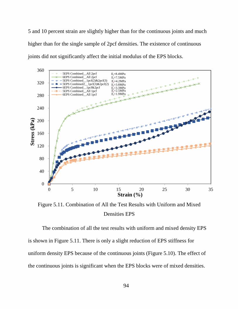
5 and 10 percent strain are slightly higher than for the continuous joints and much
higher than for the single sample of 2pcf densities. The existence of continuous
joints did not significantly affect the initial modulus of the EPS blocks.
Figure 5.11. Combination of All the Test Results with Uniform and Mixed
Densities EPS
The combination of all the test results with uniform and mixed density EPS
is shown in Figure 5.11. There is only a slight reduction of EPS stiffness for
uniform density EPS because of the continuous joints (Figure 5.10). The effect of
the continuous joints is significant when the EPS blocks were of mixed densities.
0
40
80
120
160
200
240
280
320
360
0 5 10 15 20 25 30 35
Stre
ss (k
Pa)
Strain (%)
5EPS Combined__All 2pcf6EPS Combined__All 2pcf5EPS Combined__1pcf(2)&2pcf(3)5EPS Combined2__1pcf(3)&2pcf(2)6EPS Combined__1pcf&2pcf5EPS Combined__All 1pcf6EPS Combined__All 1pcf Ei=1.9MPa
Ei=2.5MPa
Ei=4.2MPaEi=7.5MPaEi=8.4MPa
Ei=3.3MPaEi=3.8MPa
94
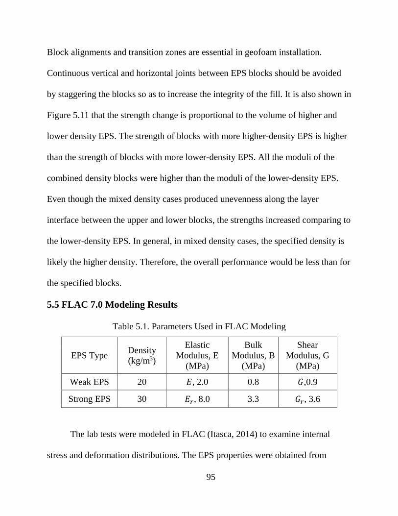
Block alignments and transition zones are essential in geofoam installation.
Continuous vertical and horizontal joints between EPS blocks should be avoided
by staggering the blocks so as to increase the integrity of the fill. It is also shown in
Figure 5.11 that the strength change is proportional to the volume of higher and
lower density EPS. The strength of blocks with more higher-density EPS is higher
than the strength of blocks with more lower-density EPS. All the moduli of the
combined density blocks were higher than the moduli of the lower-density EPS.
Even though the mixed density cases produced unevenness along the layer
interface between the upper and lower blocks, the strengths increased comparing to
the lower-density EPS. In general, in mixed density cases, the specified density is
likely the higher density. Therefore, the overall performance would be less than for
the specified blocks.
5.5 FLAC 7.0 Modeling Results
Table 5.1. Parameters Used in FLAC Modeling
EPS Type Density (kg/m3)
Elastic Modulus, E
(MPa)
Bulk Modulus, B
(MPa)
Shear Modulus, G
(MPa)
Weak EPS 20 𝐸𝐸, 2.0 0.8 𝐺𝐺,0.9
Strong EPS 30 𝐸𝐸𝑟𝑟, 8.0 3.3 𝐺𝐺𝑟𝑟, 3.6
The lab tests were modeled in FLAC (Itasca, 2014) to examine internal
stress and deformation distributions. The EPS properties were obtained from
95
previous lab test results and are shown in Table 5.1. With these parameters, FLAC
was used to model the unconfined compression test response to single and mixed
EPS geofoam density combinations.
(1) Rigid Boundary Condition
The tests conducted in the lab were unconfined compression loading by rigid end
plates that imposed uniform displacement along the plate interfaces. Therefore, to
simulate the rigid end boundary, a constant velocity of -0.000169m/s (10%/min
strain rate) was applied at the top of the sample keeping the bottom fixed. Even
though the real boundary condition applied at the top of EPS blocks was free, the
top boundary was shown fixed only due to the application of constant velocity to
displace the sample downward.
As for the mixed density modeling, interface condition were considered. FLAC
provides interfaces that are characterized by Coulomb sliding and/or tensile
separation. Interfaces have the properties of friction, cohesion, dilation, normal and
shear stiffness, and tensile strength. The normal (𝐾𝐾𝑁𝑁) and shear stiffness (𝐾𝐾𝑆𝑆) of
EPS blocks were separately determined as 1.05 × 10⁴𝑀𝑀𝑀𝑀𝑀𝑀/𝑚𝑚 and 4.7 ×
103𝑀𝑀𝑀𝑀𝑀𝑀/𝑚𝑚 using Equation 5.1 and 5.2. Joint pacing S of 0.01in was used.
Normal Stiffness: 𝐾𝐾𝑁𝑁 = 𝐸𝐸∙𝐸𝐸𝑟𝑟𝑆𝑆(𝐸𝐸𝑟𝑟−𝐸𝐸)
Equation 5.1
Shear Stiffness: 𝐾𝐾𝑆𝑆 = 𝐺𝐺∙𝐺𝐺𝑟𝑟𝑆𝑆(𝐺𝐺𝑟𝑟−𝐺𝐺)
Equation 5.2
96
Figure 5.12 and Figure 5.13 present the boundary and interface conditions of
FLAC model for the cases of mixed density EPS blocks with and without
continuous joints. For field conditions, vertical gaps may be closed in the presence
of confining pressures. The joint spacing S could be very small and even negligible.
The normal and shear stiffness would be very high. Therefore, the interface
element condition may not be important for FLAC Modeling of buried geofoam
with confining pressure.
97
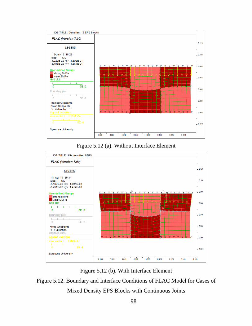
Figure 5.12 (a). Without Interface Element
Figure 5.12 (b). With Interface Element
Figure 5.12. Boundary and Interface Conditions of FLAC Model for Cases of
Mixed Density EPS Blocks with Continuous Joints
98

Figure 5.13 (a). Without Interface Element
Figure 5.13 (b) With Interface Element
Figure 5.13. Boundary and Interface Conditions of FLAC Model for Cases of
Mixed Density EPS Blocks without Continuous Joints 99
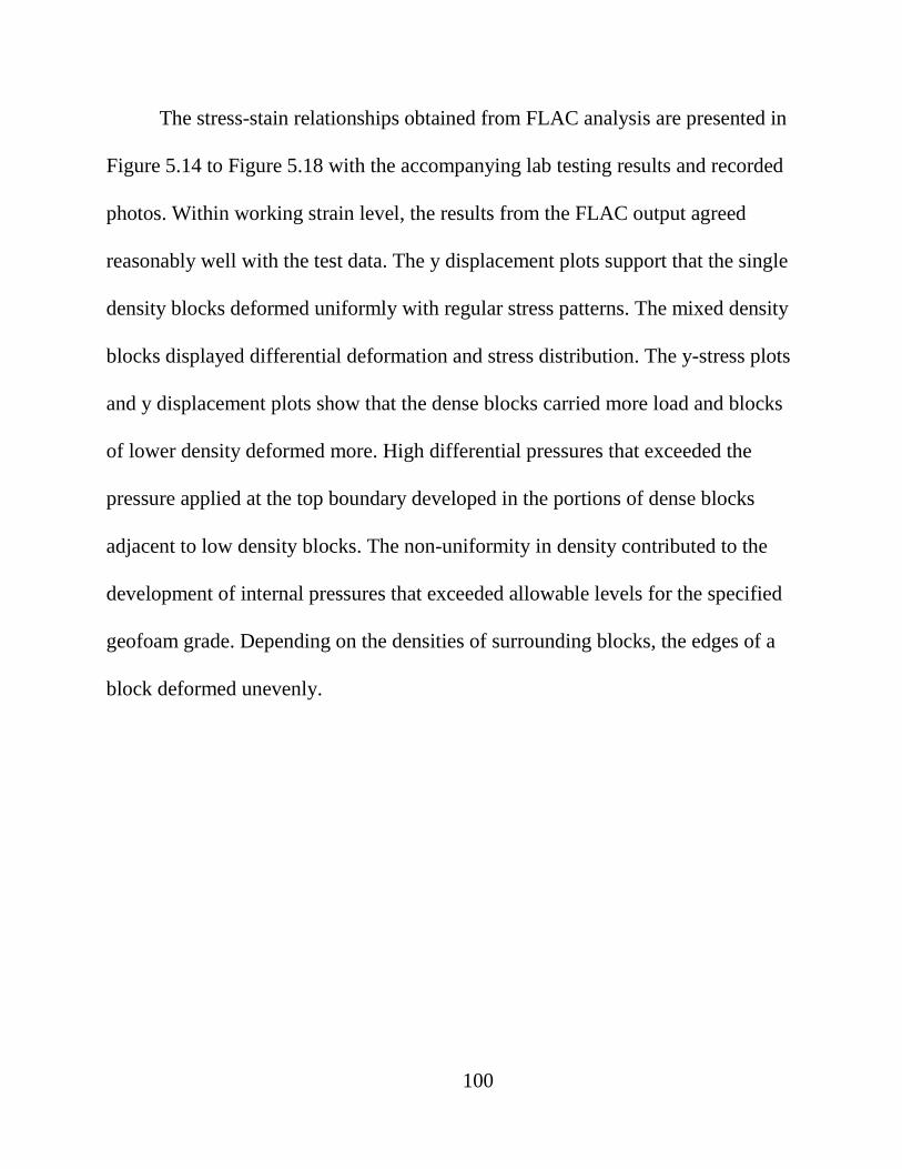
The stress-stain relationships obtained from FLAC analysis are presented in
Figure 5.14 to Figure 5.18 with the accompanying lab testing results and recorded
photos. Within working strain level, the results from the FLAC output agreed
reasonably well with the test data. The y displacement plots support that the single
density blocks deformed uniformly with regular stress patterns. The mixed density
blocks displayed differential deformation and stress distribution. The y-stress plots
and y displacement plots show that the dense blocks carried more load and blocks
of lower density deformed more. High differential pressures that exceeded the
pressure applied at the top boundary developed in the portions of dense blocks
adjacent to low density blocks. The non-uniformity in density contributed to the
development of internal pressures that exceeded allowable levels for the specified
geofoam grade. Depending on the densities of surrounding blocks, the edges of a
block deformed unevenly.
100
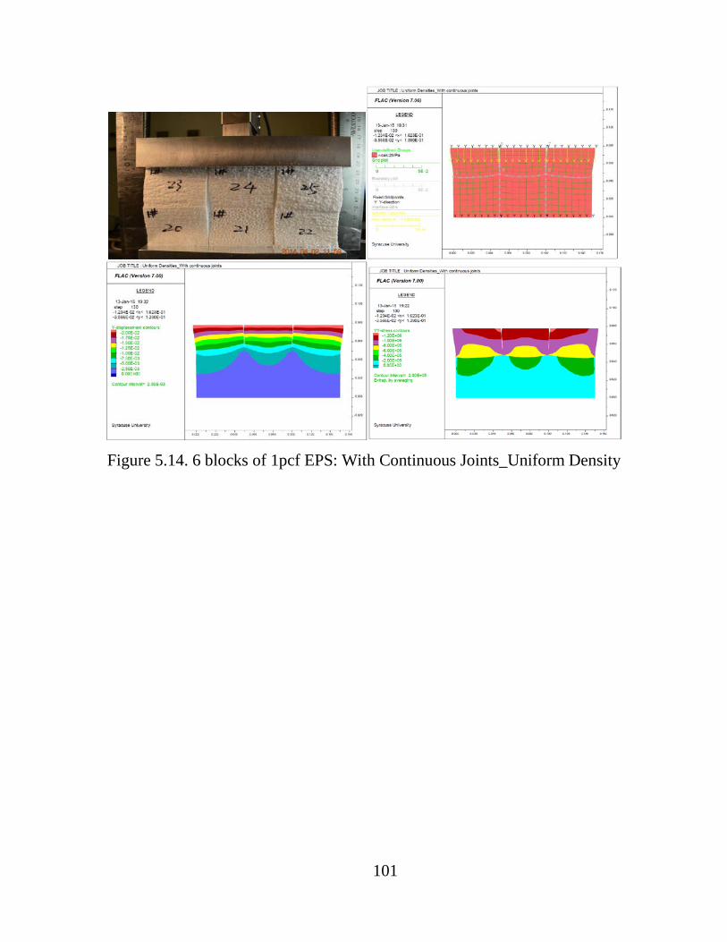
Figure 5.14. 6 blocks of 1pcf EPS: With Continuous Joints_Uniform Density
101
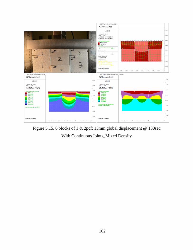
Figure 5.15. 6 blocks of 1 & 2pcf: 15mm global displacement @ 130sec
With Continuous Joints_Mixed Density
102
Figure 5.16. 5 blocks of 1pcf EPS: Without Continuous Joints_Uniform Density
103
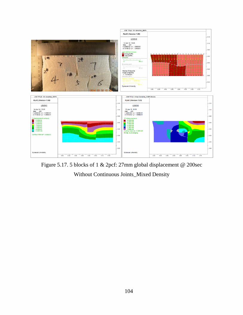
Figure 5.17. 5 blocks of 1 & 2pcf: 27mm global displacement @ 200sec
Without Continuous Joints_Mixed Density
104
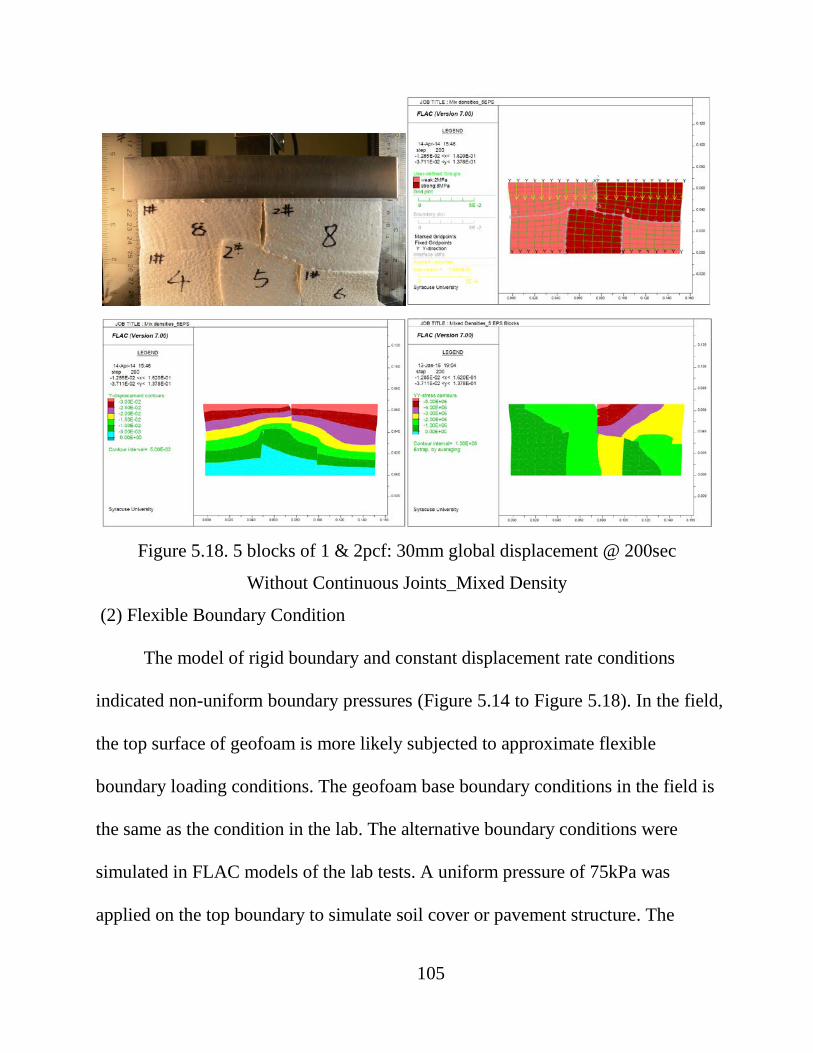
Figure 5.18. 5 blocks of 1 & 2pcf: 30mm global displacement @ 200sec
Without Continuous Joints_Mixed Density
(2) Flexible Boundary Condition
The model of rigid boundary and constant displacement rate conditions
indicated non-uniform boundary pressures (Figure 5.14 to Figure 5.18). In the field,
the top surface of geofoam is more likely subjected to approximate flexible
boundary loading conditions. The geofoam base boundary conditions in the field is
the same as the condition in the lab. The alternative boundary conditions were
simulated in FLAC models of the lab tests. A uniform pressure of 75kPa was
applied on the top boundary to simulate soil cover or pavement structure. The
105

modeling results are shown in Figure 5.19 and Figure 5.20. The modeling results
with a flexible boundary also show the low density blocks deformed more and the
high density blocks carried more load. Installing EPS blocks with mixed densities
and continuous vertical joints (Figure 5.19) result in non-uniform stress and strain
distribution and differential deformation.
Figure 5.19. FLAC Modeling Results of Mixed Densities and with Continuous
Vertical Joints Condition with Flexible Top Loading Boundary
106

Figure 5.20. FLAC Modeling Results of Mixed Densities and without Continuous
Vertical Joints Condition with Flexible Top Loading Boundary
5.6 Conclusions
Based on the lab test and FLAC modeling results, the following conclusions
can be made:
1. Stress-strain curves for combined low and high density EPS blocks lie
between stress-strain curves for all high density and all low density blocks.
107
2. EPS blocks with staggered vertical joints had higher strengths and lower
deformations than EPS blocks separated by continuous vertical joints.
3. The combined density tests show higher density EPS blocks deform much
less than adjacent low density blocks at the same load stage.
4. The lab results suggest it is important not to mix high and low density
EPS blocks in the same layer.
5. EPS blocks should be installed with staggered vertical joints to minimize
differential movements.
6. Even though the mixed density case will cause the unevenness of the
interface between the upper and lower blocks according to the images captured
during loading process, the strength increases. However, in actual cases, the high
density blocks tend to be the specified blocks. Thus the performance of the mixed
blocks would be inferior to the uniform high density specified blocks.
108
CHAPTER 6
CONCLUSIONS AND RECOMMENDATIONS
Engineering performances of EPS geofoam has been presented in this
investigation. The effect of induced anisotropy on the stress-strain behavior of EPS
geofoam, the effect of combining different EPS densities and also the different
stress-strain reactions for the condition of with or without continuous joints are
analyzed by using traditional stress-strain measurement and newly developed
ARAMIS image analysis. The following conclusions and recommendations are
made:
1. Loading and unloading cycles to max of 40% working stress did not
produce significant modulus degradation. Loading to post-yield stage and full
unloading and reloading cycles produced significant modulus degradation of up to
56~68% of initial modulus. Loading to post-yield stage and partial unloading and
reloading cycles produced much less modulus degradation than full unloading and
reloading cycles. On unloading and reloading, the proportional limit increases with
accumulated strain. The results suggested controlled pre-stressing of geofoam fill
can be beneficial in reducing initial deformations while improving the allowable
working stress range. EPS geofoam tends to develop softer reloading modulus but
continue to strain harden, and stiffen beyond the max load history level. If pre-
straining results in suppressing creep deformation, the increase in proportional
109
limit and moderate degradation in response to partial unloading and reloading
cycles may be a favorable development.
2. The optical non-contact system can accommodate any sample size and
full-scale models to directly detect displacements of selected points or image facets
at high resolution and in 3D. Synchronizing force sensing with displacement
detection, directional moduli and Poisson’s ratios can be determined from one test
sample. It was verified that the traditional way of determining modulus of EPS
blocks is conservative. The strain distribution across the face of an EPS sample is
initially uniform and becomes highly non-uniform with increasing load and strain
development. The difference of local strain are small at lower global strain level
and high at higher global strain level. For mixed density tests, the dense (2pcf) EPS
blocks were carrying more loads. As a result, the strain level was in between the
higher level for 1pcf and lower level for 2pcf. Time lapse images and video
recordings show progressive strain development for the cellular structure of EPS is
in crushing normal to the direction of loading rather than inclined shear bands as
occur for soil and other rigid materials.
3. Stress-strain curves for combined low and high density EPS blocks lie
between stress-strain curves for all high density and all low density blocks. EPS
blocks with staggered vertical joints had higher strengths and lower deformations
than EPS blocks separated by continuous vertical joints. The combined density
110

tests show higher density EPS blocks deform much less than adjacent low density
blocks at the same load stage. The lab results suggest it is important not to mix
high and low density EPS blocks in the same layer. EPS blocks should be installed
with staggered vertical joints to minimize differential movements. Even though the
mixed density case will cause the unevenness of the interface between the upper
and lower blocks according to the images captured during loading process, the
strength increases. However, in actual cases, the high density blocks tend to be the
specified blocks. Thus the performance of the mixed blocks would be inferior to
than the uniform high density specified blocks.
111
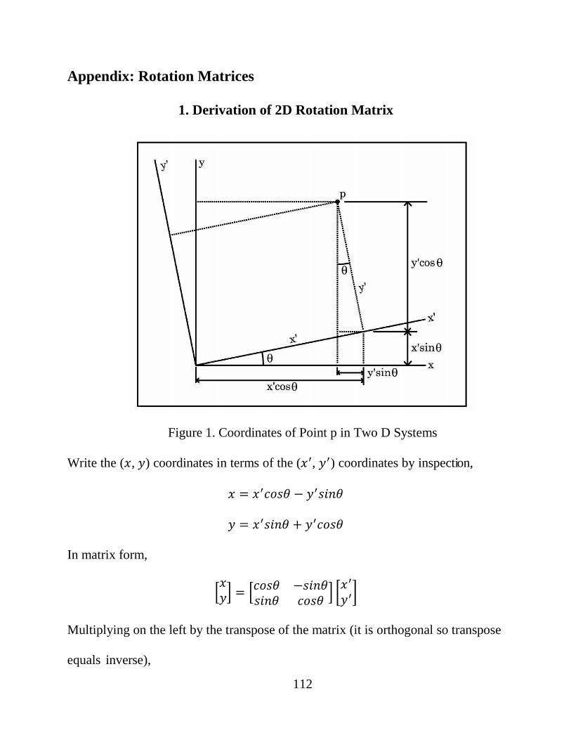
Appendix: Rotation Matrices
1. Derivation of 2D Rotation Matrix
Figure 1. Coordinates of Point p in Two D Systems
Write the (𝑥𝑥, 𝑦𝑦) coordinates in terms of the (𝑥𝑥′, 𝑦𝑦′) coordinates by inspection,
𝑥𝑥 = 𝑥𝑥′𝑐𝑐𝑐𝑐𝑐𝑐𝑐𝑐 − 𝑦𝑦′𝑐𝑐𝑖𝑖𝑠𝑠𝑐𝑐
𝑦𝑦 = 𝑥𝑥′𝑐𝑐𝑖𝑖𝑠𝑠𝑐𝑐 + 𝑦𝑦′𝑐𝑐𝑐𝑐𝑐𝑐𝑐𝑐
In matrix form,
�𝑥𝑥𝑦𝑦� = �𝑐𝑐𝑐𝑐𝑐𝑐𝑐𝑐 −𝑐𝑐𝑖𝑖𝑠𝑠𝑐𝑐
𝑐𝑐𝑖𝑖𝑠𝑠𝑐𝑐 𝑐𝑐𝑐𝑐𝑐𝑐𝑐𝑐 � �𝑥𝑥′𝑦𝑦′�
Multiplying on the left by the transpose of the matrix (it is orthogonal so transpose
equals inverse),
112

�𝑥𝑥′
𝑦𝑦′� = � 𝑐𝑐𝑐𝑐𝑐𝑐𝑐𝑐 𝑐𝑐𝑖𝑖𝑠𝑠𝑐𝑐−𝑐𝑐𝑖𝑖𝑠𝑠𝑐𝑐 𝑐𝑐𝑐𝑐𝑐𝑐𝑐𝑐� �
𝑥𝑥𝑦𝑦�
This represents the basic equation describing 2D rotations. Note that the sense of
the angle 𝑐𝑐 is defined by the right hand rule. A positive rotation means that if the
thumb of the right hand is pointed along the positive direction of the rotation axis
(𝑧𝑧), then the fingers curl in the positive direction, i.e. counterclockwise. We will
adopt the convention that rotation means a rotation of the coordinate axes, not the
point. If the axes are rotated counterclockwise, then the point itself appears to
rotate clockwise, with respect to fixed axes. See Figure 2 below.
Figure 2. Equivalence of Rotating Axes in one Direction, and a Point in the
Opposite Direction
113

2. Derivation of 3D Elementary Rotation Matrices
We can extend the prior development into 3D rotations by constructing
elementary 3D rotation matrices. The elementary 3D rotation matrices are
constructed to perform rotations individually about the three coordinate axes. We
begin with the rotation about the 𝑧𝑧-axis (𝑘𝑘, or kappa), since it is virtually identical
to what was just developed. We keep the same 𝑥𝑥𝑦𝑦 transformation but add an
identity transformation for the 𝑧𝑧-coordinate, since it will not change during a
rotation about the 𝑧𝑧-axis. See Figure 3.
�𝑥𝑥′𝑦𝑦′𝑧𝑧′� = �−
𝑐𝑐𝑐𝑐𝑐𝑐𝜅𝜅 𝑐𝑐𝑖𝑖𝑠𝑠𝜅𝜅 0𝑐𝑐𝑖𝑖𝑠𝑠𝜅𝜅 𝑐𝑐𝑐𝑐𝑐𝑐𝜅𝜅 0
0 0 1� �𝑥𝑥𝑦𝑦𝑧𝑧� = 𝑅𝑅𝑘𝑘 �
𝑥𝑥𝑦𝑦𝑧𝑧�
Figure 3. Rotation about the 𝑧𝑧-axis
114
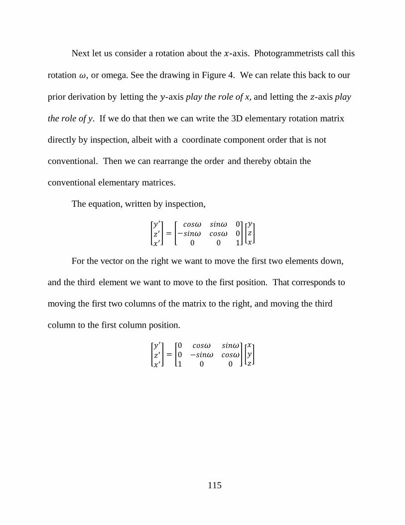
Next let us consider a rotation about the 𝑥𝑥-axis. Photogrammetrists call this
rotation 𝜔𝜔, or omega. See the drawing in Figure 4. We can relate this back to our
prior derivation by letting the 𝑦𝑦-axis play the role of x, and letting the 𝑧𝑧-axis play
the role of y. If we do that then we can write the 3D elementary rotation matrix
directly by inspection, albeit with a coordinate component order that is not
conventional. Then we can rearrange the order and thereby obtain the
conventional elementary matrices.
The equation, written by inspection,
�𝑦𝑦′𝑧𝑧′𝑥𝑥′� = �−
𝑐𝑐𝑐𝑐𝑐𝑐𝜔𝜔 𝑐𝑐𝑖𝑖𝑠𝑠𝜔𝜔 0𝑐𝑐𝑖𝑖𝑠𝑠𝜔𝜔 𝑐𝑐𝑐𝑐𝑐𝑐𝜔𝜔 0
0 0 1� �𝑦𝑦𝑧𝑧𝑥𝑥�
For the vector on the right we want to move the first two elements down,
and the third element we want to move to the first position. That corresponds to
moving the first two columns of the matrix to the right, and moving the third
column to the first column position.
�𝑦𝑦′𝑧𝑧′𝑥𝑥′� = �
0 𝑐𝑐𝑐𝑐𝑐𝑐𝜔𝜔 𝑐𝑐𝑖𝑖𝑠𝑠𝜔𝜔0 −𝑐𝑐𝑖𝑖𝑠𝑠𝜔𝜔 𝑐𝑐𝑐𝑐𝑐𝑐𝜔𝜔1 0 0
� �𝑥𝑥𝑦𝑦𝑧𝑧�
115
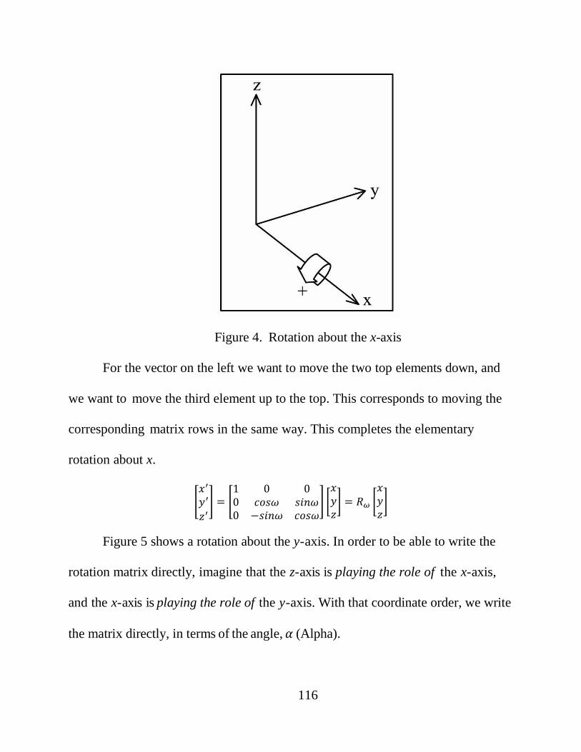
Figure 4. Rotation about the x-axis
For the vector on the left we want to move the two top elements down, and
we want to move the third element up to the top. This corresponds to moving the
corresponding matrix rows in the same way. This completes the elementary
rotation about x.
�𝑥𝑥′𝑦𝑦′𝑧𝑧′� = �
1 0 00 𝑐𝑐𝑐𝑐𝑐𝑐𝜔𝜔 𝑐𝑐𝑖𝑖𝑠𝑠𝜔𝜔0 −𝑐𝑐𝑖𝑖𝑠𝑠𝜔𝜔 𝑐𝑐𝑐𝑐𝑐𝑐𝜔𝜔
� �𝑥𝑥𝑦𝑦𝑧𝑧� = 𝑅𝑅𝜔𝜔 �
𝑥𝑥𝑦𝑦𝑧𝑧�
Figure 5 shows a rotation about the y -axis. In order to be able to write the
rotation matrix directly, imagine that the z-axis is playing the role of the x-axis,
and the x-axis is playing the role of the y -axis. With that coordinate order, we write
the matrix directly, in terms of the angle, 𝛼𝛼 (Alpha).
116

�𝑧𝑧′𝑥𝑥′𝑦𝑦′� = �−
𝑐𝑐𝑐𝑐𝑐𝑐𝛼𝛼 𝑐𝑐𝑖𝑖𝑠𝑠𝛼𝛼 0𝑐𝑐𝑖𝑖𝑠𝑠𝛼𝛼 𝑐𝑐𝑐𝑐𝑐𝑐𝛼𝛼 0
0 0 1� �𝑧𝑧𝑥𝑥𝑦𝑦�
In order to rearrange the order of the vector on the right, we must slide the
last two matrix columns left, and move the leftmost column over to the right.
�𝑧𝑧′𝑥𝑥′𝑦𝑦′� = �
𝑐𝑐𝑖𝑖𝑠𝑠𝛼𝛼 0 𝑐𝑐𝑐𝑐𝑐𝑐𝛼𝛼𝑐𝑐𝑐𝑐𝑐𝑐𝛼𝛼 0 −𝑐𝑐𝑖𝑖𝑠𝑠𝛼𝛼
0 1 0� �𝑥𝑥𝑦𝑦𝑧𝑧�
Figure 5. Rotation about the y-axis
In order to put the elements of the vector on the left into the conventional x
y z order, we must slide the bottom two matrix rows up, and move the top row
down to the bottom.
117

�𝑥𝑥′𝑦𝑦′𝑧𝑧′� = �
𝑐𝑐𝑐𝑐𝑐𝑐𝛼𝛼 0 −𝑐𝑐𝑖𝑖𝑠𝑠𝛼𝛼0 1 0
𝑐𝑐𝑖𝑖𝑠𝑠𝛼𝛼 0 𝑐𝑐𝑐𝑐𝑐𝑐𝛼𝛼� �𝑥𝑥𝑦𝑦𝑧𝑧� = 𝑅𝑅𝛼𝛼 �
𝑥𝑥𝑦𝑦𝑧𝑧�
This completes the elementary rotation about y. These elementary matrices
can be combined to create any 3D rotation. In photogrammetry the usual order of
the rotations is lastly kappa (z) first, then alpha (y), and omega (x). A matrix
applied first is on the right, therefore the general composite rotation is,
𝑅𝑅 = 𝑅𝑅𝑘𝑘𝑅𝑅𝛼𝛼𝑅𝑅𝜔𝜔
Writing out all of the elements of the composite rotation we get,
𝑅𝑅 = �−𝑐𝑐𝑐𝑐𝑐𝑐𝜅𝜅 ∙ 𝑐𝑐𝑐𝑐𝑐𝑐𝛼𝛼 𝑐𝑐𝑖𝑖𝑠𝑠𝜅𝜅 ∙ 𝑐𝑐𝑐𝑐𝑐𝑐𝜔𝜔 + 𝑐𝑐𝑐𝑐𝑐𝑐𝜅𝜅 ∙ 𝑐𝑐𝑖𝑖𝑠𝑠𝛼𝛼 ∙ 𝑐𝑐𝑖𝑖𝑠𝑠𝜔𝜔 𝑐𝑐𝑖𝑖𝑠𝑠𝜅𝜅 ∙ 𝑐𝑐𝑖𝑖𝑠𝑠𝜔𝜔 − 𝑐𝑐𝑐𝑐𝑐𝑐𝜔𝜔 ∙ 𝑐𝑐𝑖𝑖𝑠𝑠𝛼𝛼 ∙ 𝑐𝑐𝑐𝑐𝑐𝑐𝜅𝜅𝑐𝑐𝑖𝑖𝑠𝑠𝜅𝜅 ∙ 𝑐𝑐𝑐𝑐𝑐𝑐𝛼𝛼 𝑐𝑐𝑐𝑐𝑐𝑐𝜅𝜅 ∙ 𝑐𝑐𝑐𝑐𝑐𝑐𝜔𝜔 − 𝑐𝑐𝑖𝑖𝑠𝑠𝜅𝜅 ∙ 𝑐𝑐𝑖𝑖𝑠𝑠𝛼𝛼 ∙ 𝑐𝑐𝑖𝑖𝑠𝑠𝜔𝜔 𝑐𝑐𝑖𝑖𝑠𝑠𝜔𝜔 ∙ 𝑐𝑐𝑐𝑐𝑐𝑐𝜅𝜅 + 𝑐𝑐𝑐𝑐𝑐𝑐𝜔𝜔 ∙ 𝑐𝑐𝑖𝑖𝑠𝑠𝛼𝛼 ∙ 𝑐𝑐𝑖𝑖𝑠𝑠𝜅𝜅
𝑐𝑐𝑖𝑖𝑠𝑠𝛼𝛼 −𝑐𝑐𝑖𝑖𝑠𝑠𝜔𝜔 ∙ 𝑐𝑐𝑐𝑐𝑐𝑐𝛼𝛼 𝑐𝑐𝑐𝑐𝑐𝑐𝜔𝜔 ∙ 𝑐𝑐𝑐𝑐𝑐𝑐𝛼𝛼�
118

References
ASTM D 6817, ASTM D 1621, C 165, EN 826 or ISO 844.
Taylor, D. W. (1948), “Fundamental of Soil Mechanics”, John Wiley and Sons,
Inc., New York, NY.
Coleman, T.A., (1974), “Polystyrene Foam Is Competitive Lightweight Fill”, Civil
Engineering, Vol. 44, No.2, pp. 68-69.
Aabøe, R., (1981), “Plastic Foam in Road Embankments, Norwegian Road
Research Laboratory, Oslo, Norway.
Aabøe, R., (1985), “Plastic Foam in Road Embankments: Experience with
Expanded Polystyrene as a Lightweight Fill Material in Road
Embankments”, Norwegian Road Research Laboratory, Oslo, Norway.
Aabøe, R., (1987), “13 Years of Experience with Expanded Polystyrene as a
lightweight Fill Material in Road Embankments”, Norwegian Road Research
Laboratory, Publication No. 61, Oslo, Norway, pp. 21-27.
van Dorp, T., (1988), “Expanded Polystyrene Foam as Light Fill and Foundation
Material in Road Structures”, International Congress on Expanded
Polystyrene, Pre-print, Milan, Italy, 19p.
Yeh, S., T., and Gilmore, J., B., (1989), “Application of EPS for Slide Correction,
Stability and Performance of Slopes and Embankments II, ASCE
Geotechnical Special Publication, NY, USA, No. 31, pp. 1444-1456.
Eriksson, L., and Trank, R., (1991), “Properties of Expanded Polystyrene,
Laboratory Experiments”, Swedish Geotechnical Institute, Linköping,
Sweden.
BASF Corp., (1993), “Styropor Foam as a Lightweight Construction Material for
Base-Course”, Styropor Technical Information, BASF Corp., Ludwigshafen,
Germany.
119
Mimura, C., S., and Kimura, S., A., (1995), “A Lightweight Solution”, Geosynthet-
ics 95 Conference Proceedings, Vol. 1, Nashville Tennessee, USA, pp. 39-
51.
Thompsett, D., Walker, A., Radley, R., and Grieveson, B., (1995), “Design and
Construction of Expanded Polystyrene Embankments”, Construction and
Building Materials, U.K., Vol. 9, No. 6, pp. 403-411.
Frydenlund, T., E., and Aabøe, R., (1996), “Expanded Polystyrene-The Light
solution”, Proceedings of the International Symposium on EPS Construction
Method, Tokyo, Japan, pp 31-46.
van Dorp, T., (1996), “Building on EPS Geofoam in the “Low-Lands” Experiences
in the Netherlands”, Proceedings of the International Symposium on EPS
Construction Method, Tokyo, Japan, pp. 59-69.
Sun, M.C., (1997), “Engineering Behavior of Geofoam (Expanded Polystyrene)
and Lateral Pressure Reduction in Substructures”, Master’s Thesis, Syracuse
University, New York.
Duškov, M., (1997), “EPS as a Light Weight Sub-Base Material in Pavement
Structures”, Ph.D. Thesis, Delft University of Technology, Delft, the
Netherlands.
Negussey, D., (1997), “Properties & Applications of Geofoam”, Society of the
Plastic Industry, Inc., Washington, D.C., USA.
BASF Corp., (1997), “Styropor Technical Information”, Technical Information,
BASF Corp., Germany.
Horvath, J., (1998), “Mathematical Modeling of the Stress-Strain-Time Behavior
of Geosynthetics Using the Findley Equation: General Theory and
Application to EPS-Block Geofoam”, Manhattan College Research Report
No. CE/GE-98-3, Bronx, N.Y.
120
Negussey, D., (1998), “Putting Polystyrene to Work”, Civil Engineering, American
Society of Civil Engineering, NY, USA, Vol. 68, No. 3, pp. 65-67.
GeoTech, (1998), “Geofoam Compressible Inclusions: A Conceptual Guide to
Analysis and Design”, GeoTech System Corporation, VA, USA.
BASF Corporation (1998), “Styropor Foam as a Lightweight Construction
Material for Road Base-Courses,” Styropor Technical Information,
Ludwigshafen, Germany.
Jutkofsky, W., S., Teh, S., J., and Negussey, D., (2000), “Stabilization of an
Embankment Slope with Geofoam”, Transportation Research Board, 79th
Annual Meeting, Paper No. 00-1315, Washington, D.C., USA.
Cole, B., (2000), “How EPS Foam Saved the City of Issaquah 1.2 Million Dollars
and One Year of Construction Time”, Preprint Paper, Syracuse Geofoam
Seminar, Salt Lake City, Utah, USA.
Elragi, A., (2000), “Selected Engineering Properties and Applications of EPS
Geofoam”, Ph.D. Thesis, State University of New York, Syracuse, N.Y.
Sheeley, M., (2000), “Slope Stabilization Utilizing Geofoam”, Master’s Thesis,
Syracuse University, New York.
Elragi, A., Negussey, D., and Kyanka, G., (2000), “Sample Size Effects on the
Behavior of EPS Geofoam”, Proceedings of the Soft Ground Technology
Conference, ASCE Geotechnical Special Publication 112, Noordwijkerhout,
the Netherlands.
Dimitrios K. Atmatzidis, Emmanuel G. Missirlis and Dimitrios A. Chrysikos,
(2001), “An Investigation of EPS Geofoam Behavior in Compression”, EPS
geofoam 2001 3rd International Conference.
Srirajan, S., (2001), “Recycled Content and Creep Performance of EPS Geofoam
in Slope Stabilization”, Master’s Thesis, Syracuse University, New York.
121
Anasthas, N., (2001), “Young’s Modulus by Bending Tests and Other Engineering
Properties of EPS Geofoam”, Master’s Thesis, Syracuse University,
Syracuse, NY.
Negussey, D. (2007), “Design Parameters for EPS Geofoam”, Soils and
Foundations, Japanese Geotechnical Society, Vol. 47, No. 1, pp. 161 - 170.
Lingwall, B. N. (2011), “Development of an Expanded Polystyrene Geofoam
Cover System for Pipelines at Fault Crossings, Dissertation”, University of
Utah, Department of Civil and Environmental Engineering, Salt Lake City,
Utah.
T Ahmed Awol, (2012), “A Parametric Study of Creep on EPS Embankments”,
Master’s Thesis, Norwegian University of Science and Technology.
GeoJac user manual
ARAMIS user manual
FLAC 7.0 user manual
122


