
Journal of Laboratory Chemical Education 2017, 5(4): 55-66
DOI: 10.5923/j.jlce.20170504.01
Study of UV Filters as an in silico (QSAR) Graduate
Project
D. González-Arjona1,*
, G. López-Pérez1, A. Gustavo González
2, M. M. Domínguez
1, W. H. Mulder
3
1Department of Physical Chemistry, Universidad de Sevilla, Sevilla, Spain 2Department of Analytical Chemistry, Universidad de Sevilla, Sevilla, Spain 3Department of Chemistry, University of the West Indies, Kingston, Jamaica
Abstract A simplified in silico QSAR study, involving more than 50 molecules that are commonly used as UV filters in
sunscreens, is presented. Details of methodology are described and illustrated step by step and the use of available tools is
demonstrated, including data set selection, generation of molecular structure files, selection of computational methods,
assessment of the relative importance of molecular properties, generation of theoretical UV-Vis spectra and construction of a
QSAR model. With the aim of introducing the QSAR methodology at undergraduate level, some simplifications have been
made. Multiple Linear Regression (MLR) has been selected as a modeling strategy to correlate the molecular descriptors and
the sunlight blocking effect. The full area under the UV-Vis spectrum has been used as a simple measure of the protection
factor. Theoretical UV-Vis spectra have been generated by using the configuration interaction (CI) approximation. The
ground state molecular geometry has been optimized by the semi-empirical ZINDO computational method. Inclusion of a
solvent model in the optimization of molecular geometry to account for solvatochromic effects has not been considered. On
the other hand, total number of rings, number of aromatic rings, molecular dipole moment and HOMO/LUMO energy gap,
are considered to be significant parameters in the MRL model. The HOMO/LUMO energy gap is the variable of choice when
optimized single linear regression analysis is carried out separately for each of the functional groups of the compounds. The
great variety of tools and procedures used in building QSAR models has been found to provide ample scope for active
involvement by the students, exposing them to a fairly broad array of modern methods in areas like drug discovery and
toxicology.
Keywords QSAR, Sunscreens, UV-VIS absorption, Graduation projects
1. Introduction
More than half a century has passed since Hansch et al [1]
laid the foundations of the modern methodology of
―Quantitative Structure-Activity Relationships‖ (QSAR),
initially building on the work of Polanyi and subsequently
Hammett who introduced the concept of ―Linear Free
Energy Relationships‖ (LFERs), by correlating the
chemical structure of the phenoxyacetic acids with their
biological activity in plant growth. Since then, QSAR has
evolved to a point where it provides reliable, statistically
predictive models.
Designing a chemical compound that possesses certain
properties is usually very complicated relative to the effort
involved in synthesizing a particular molecular structure.
Although it may be relatively easy to deduce a reaction
mechanism from a knowledge of molecular structure, it is
often far more difficult to predict its properties based on this
* Corresponding author:
[email protected] (D. González-Arjona)
Published online at http://journal.sapub.org/jlce
Copyright © 2017 Scientific & Academic Publishing. All Rights Reserved
structure. Whereas the reactivity appears as an intrinsic
characteristic of the molecule this is not necessarily true for
physicochemical or biological properties. The peculiar
properties and behavior of a compound depend on both its
internal structure and the molecular environment in which it
finds itself. The surroundings interact with the entire
molecule and more strongly so with specific sites. However,
unlike chemical reactions, these interactions are relatively
weak and do not lead to the breaking or formation of
chemical bonds. Therefore, the modeling needed to relate
the structure and a particular activity quantitatively, QSAR,
is not a trivial task.
The use of QSAR models for the screening of
chemical/biological products is a matter of great interest in
both the chemical and pharmaceutical industry, toxicology,
medicine, environmental studies, etc. The QSAR modeling
method appears as one of the most useful tools in the
understanding and prediction of properties and effects of
chemical/biological compounds in the areas of environment
and health. This methodology constitutes an efficient and
operative means of assessing chemical hazards. In addition,
the use of QSAR offers other advantages, such as low cost,
high degree of investment recovery and it may even reduce

56 D. González-Arjona et al.: Study of UV Filters as an in silico (QSAR) Graduate Project
the need for using animals in laboratory testing of new
drugs. All these applications have attracted the growing
interest from government agencies for in silico predictions
[2, 3]. Clearly, QSAR modeling is a multidisciplinary
subject, which combines aspects from computer science,
chemistry, statistics (cheminformatics) and knowledge of
disciplines, particularly toxicology, that explore the activity
of chemicals as it relates to health and environment.
The mechanism underlying the protection by sunscreens
is well known. It primarily involves absorption of UV light
by electrons in a molecule‘s frontier orbital [4]. Thus, the
active compound in sunscreens protects the skin from
sunburn by blocking UV radiation. The extent of this action
can be evaluated experimentally based on the UV-Vis
absorption spectrum. Therefore, a knowledge of the nature
of UV filter action, the straightforward identification of a
target function (UV-Vis spectral area), together with the
relative ease with which molecules of intermediate size can
be modeled, makes the group of molecules that act as UV
filters an ideal object for a QSAR-type study.
With the aim of introducing the QSAR methodology at
undergraduate level, this paper describes a simplified in
silico QSAR study for different UV filters. The model is
developed using calculated numerical molecular descriptors
that encode information about each molecular structure.
From the different modeling strategies, the simple Multiple
Linear Regression (MLR) has been selected to correlate the
molecular descriptors and the sunlight blocking effect, in
this case the full area under the UV-Vis spectrum. In order
to allow completion of the project within a reasonable time,
some simplifications have been made to obtain the
molecular descriptors. Thus, the theoretical method
employed to generate both the molecular descriptors and the
UV-Vis spectral area are based on semi-empirical quantum
chemical methods. Moreover, the solvent effect is not taken
into account [5]. Modeling of the solvatochromic effect is a
complex undertaking and is outside the didactical scope of
the present paper [6]. Therefore, the conclusions that can be
drawn are somewhat limited. Notwithstanding, the basic
steps in QSAR methodology, viz., the building up and
optimization of 3D molecular structures, generation and
selection of descriptors and model construction and
validation are demonstrated and analyzed.
This paper therefore explores the quantitative relationship
between absorption in the UV-Vis region with the chemical
structure of UV filters, without taking into account possible
spectral shifts due to the presence of a solvent.
2. Methodology
The sun protection mechanism using organic chemicals
is based on the strong absorption of UV light by these
molecules. Therefore, the molecular energy gap for the
frontier orbital set close to HOMO-LUMO should have a
value in the UV-Vis range. This energy gap can be realized
with aromatic compounds having conjugated C=C double
bonds and other diverse functional groups. The UV-Vis
absorption interval and strength can be modified by varying
the type and position of molecular substituents. The entire
project can be developed in several stages.
2.1. Data Set Selection
The selection of compounds that constitute the data set
should be the first step of the project. Mainly seven different
classes of organic compounds are commonly employed as
active UV filters, Figure 1, shows their basic schematic
structures. The compound data set for this study was selected
from the globally approved list of UV-Vis filters [7, 8].
Figure 1. Schematics structures of different classes of organic compounds,
containing conjugated double bonds, frequently used as UV filters
The set contains five p aminobenzoate derivatives
(PABAs), twelve benzophenone derivatives, six camphor
derivatives, three dibenzoylmethane derivatives, eleven
cinnamate derivatives, six salicylate derivatives, ten
N-heterocyclic derivatives (imidazole, triazine,
benzotriazole, …), one anthranilate and two miscellaneous
compounds (beta-carotene and melanin). The table of data
can be obtained from the authors upon request.
2.2. Molecular Computer File Generation
For each compound, a computer file containing the
molecular structure readable by computational molecular
programs should be generated. Common molecular files read
by the majority of the computational chemistry programs are
the mol file, MDL and structure data file, SDF [9].
Computational Chemistry for Chemistry Educators [10],
offers information and resources for molecular modeling,
with systematic instructions for molecular modeling with
different softwares. From the name of each organic
compound, a computer file was generated containing the 3D
initial molecular structure. Different web resources can be
employed to obtain the text file containing the molecular
structure, from the IUPAC name and/or using the ―simplified
molecular-input line-entry system‖, SMILES [11]. To avoid
issues arising from different nomenclature and/or isotopes,
each compound is identified by its unique CAS registration
number [12]. This registry can be obtained from CACTUS
(CADD Group Chemoinformatics Tools and User Services)
[13]. From CAS a standard molecular file can be exported
using the ChemSpider [14], ChemCell [15], now also
available on Google Spreadsheets, or Chemicalize [16] web

Journal of Laboratory Chemical Education 2017, 5(4): 55-66 57
resources. Among them, ChemSpider, Chemicalize and
PubChem are recommended, they offer web links that give
access to estimates of assorted molecular properties, or
descriptors in QSAR nomenclature, from its structure:
ACD/Labs [17], EPISuite [18], ChemAxon [19] and Mcule
[20].
2.3. Theoretical UV-Vis Spectra and Selection of
Computational Method
The sunblock protection efficiency is usually
characterized by a test in vivo. Estimation of the sun
protection factor, SPF, is based on the ratio of the minimum
erythematic dose between protected and unprotected skin.
The comparable parameter used in vitro does not have a
unique and widely accepted definition. In this paper, the
modified parameter defined by UV area per unit of
wavelength [21], recommended based on FDA regulations
[7], is used:
2
1
2 1
UV area per unit of
( )
λ (L/(mol cm)
d
(1)
where () is the extinction coefficient and is the
wavelength. This target parameter can be easily estimated
from experimental or theoretically generated UV-Vis
spectra.
The theoretical UV-spectrum can be generated by
computational methods using the approximation known as
configuration interaction, CI, [22]. The transition energy
between the ground and the excited states are computed for
the same geometry, that of the ground state. This energy is
given usually as a wavelength for each allowed electronic
transition. The relative intensity for each transition is related
to the change in the dipolar moment strength and is reported
as the oscillator strength for each electronic transition [23].
Forbidden transitions have an oscillator strength value close
to zero. For each active transition (i), the extinction
coefficient is produced as a Gaussian band shape, with a
constant half-width (approx. 0.4 eV) by using the method
proposed in Gaussian Tech Notes [24]:
2max, max,8
-1
-1 7 -1 3 1
1 1 (nm)( ) 1.3062974 10 exp
(cm )
0.4eV=1 3099.6nm 10 3099.6 cm 3.22622 10 cm
i ii
f
(2)
where fmax,i and max,i are the oscillator strength and the
wavelength (nm) of the electronic state i, respectively.
The full spectrum can be easily convoluted by adding all
active transitions in the UV-Vis energy interval:
( ) ( )i ii
(3)
Finally, the UV area is obtained from the
spreadsheet-generated spectra by integration using the
trapezoid rule.
The ground state molecular geometry can be optimized by
several computational methods: molecular mechanical,
semi-empirical [25] and by Density Functional Theory (DFT)
[26].
Additionally, the solvatochromic effect is an experimental
complication in vitro when we want to compare the sunblock
effectiveness in vivo [5]. A deeper theoretical study should
be performed in order to obtain UV-Vis spectra closer to
those obtained experimentally. Nevertheless, this
consideration is outside the scope of the present paper, which
is meant to be an introduction to the QSAR methodology at
the undergraduate level.
2.4. Estimating Molecular Properties
The ability to predict properties depends strongly on an
appropriate choice of descriptors. There is a variety of
molecular properties that can be used in QSAR. They can be
classified as physicochemical [27, 28] and topological [29],
so that in turn they can be divided into groups [30-32]:
• Constitutional (number and type of atoms, rings,
MW, ...)
• Topological (indices that represent the structure using
graphs)
• Geometric (Areas, volumes, ...)
• Mechanical (moments of inertia, …)
• Electrostatic (polarizability, partial charge, dipole
moment, ...)
• Quantum (frontier molecular orbitals, free valence,
bond order, electronic energy, electrostatic
interaction, ...)
• Thermodynamic (heat of formation, heat capacity, ...)
Nevertheless, there is a wide variety of software
applications to obtain molecular descriptors: Codessa Pro
[33], Dragon 6 [34], CORINA Symphony [35], and
Molecular Operating Environment [36]. Most of them
provide more than 1000 descriptors for any molecule.
However, the use of a large number of descriptors in the
construction of the model has, in addition to increasing
computing time, two disadvantages: increase of ‗noise‘, due
to the use of some correlated descriptors, and model
‗over-training‘. The latter tend to produce models with
low predictive power. Nevertheless, most of the
above-mentioned software provides tools for fast data
screening to obtain the most significant descriptors,
minimizing the above-mentioned adverse effects.
2.5. QSAR Model Construction
The first stage in the model building process will be the
selection of variables (properties) that could contribute
significantly to the model as well as the estimation of their
level of importance.
These properties can be grouped in matrix form, where
each column is associated with a specific property and each
row corresponds to a chemical compound. These properties
are considered as independent variables, termed an X matrix.
An additional column is incorporated containing the
dependent variable: a molecular property (experimentally

58 D. González-Arjona et al.: Study of UV Filters as an in silico (QSAR) Graduate Project
determined or theoretically calculated) to be replicated by
the model, the Y matrix. The analysis of this matrix equation
is performed depending on the types of variables and their
mathematical relationship. Thus, the following types of
fundamental modeling strategies have been considered in the
chemometric literature [37, 38]:
• MLR, Multiple Linear Regression
• PCR, Principal Component Regression
• PLS, Partial Least Squares
• TFA, Target Factor Analysis
• ANN, Artificial Neural Networks
• SVM, Support Vector Machines
If it can be assumed that the selected independent
properties mainly contribute linearly to the model, the
multiple linear regression (MLR) based on the least squares
method should be the model technique of choice. This model
can only be applied when the variables have low synergy
among them, and no quadratic terms need to be considered.
With a view to the pedagogical scope of the project,
students mainly employed MLR which can also be easily
handled by Excel. Therefore, the MLR model equation, in
matrix format, will be:
Y X B E (4)
where Y is the dependent variable matrix, in this case, the UV
area per unit of wavelength; X is the independent variable
matrix, containing molecular properties; B corresponds to
the regression coefficient matrix, and E is associated to the
residual error matrix.
The regression coefficient matrix, B , the response
matrix Y and residual error matrix can be estimated by
least squares analysis:
1T T T T
1T T
Y X B X Y X X B B X X X Y
Y X B X X X X Y H Y E Y Y
(5)
where the superscript T stands for the transposed matrix and
the superscript -1 for the inverse matrix operation,
respectively. The tests for degrees of significance for the
linear model and for the coefficients are performed by the
statistics Snedecor‘s F and Student's t, respectively [39].
Additionally, application of the MLR model has some
statistical prerequisites: the residuals should be normally
distributed, with a constant variance and not show any trends
when plotted against any independent variable. These
prerequisites can be checked by any statistical software, like
SPSS [40] or Statistica [41]. These statistical tools can also
assist in the model building by including or dropping
variables by stepping forward or backward in the model,
respectively.
Furthermore, a severe problem in using the MLR
procedure occurs if there is a degree of measurable
correlation between some of the supposedly independent
selected variables. In particular, difficulties arise in the
calculation of the inverse of the correlation matrix:
TC X X (6)
Each element in the correlation matrix indicates the degree
of correlation between the two variables. All diagonal
elements are equal to unity, expressing the complete
correlation for each variable with itself. Entries of the
correlation matrix that are close to zero is an indication that
the corresponding two variables are uncorrelated. Several
strategies can be employed to minimize the correlation issues.
The correlation matrix analysis is the simplest way, selecting
one variable from each group that is highly correlated
(absolute values higher than 0.6) and dropping the rest of the
group. Nevertheless, this strategy can lead to the loss of some
information contained in the correlated variables. Therefore,
more complex strategies of modelling should be performed
such as principal component regression or partial least
squares.
3. Results and Discussion
After compound selection, the molecular file with the
molecular structure was generated from the web facilities
described above.
In the present project the CAChe 7.5 software as
―all-in-one‖ [42] has been employed. CAChe,
computer-aided chemistry, is a 3D molecular modeling tool
environment capable to build up molecules. The program
performs molecular calculations, named ―experiments‖,
using classical and quantum mechanical theories providing
electronic properties of the optimized molecular geometry.
Moreover, the software provides a separate ―ProjectLeader‖,
as spreadsheet interface to perform batch-processing
calculations for several chemical samples at the same time
(structures, properties, statistical analyses, multiple linear
regression, calculations based on customizable equations …).
This separate tool is specially adequate and comfortable to
perform QSAR studies. Using this spreadsheet interface the
table with the molecular properties for each molecule can be
built up.
Table 1. Selected molecular properties for the Sunscreens. Procedures and literature from [42]
Molecular Weight
Count: Atoms (Nitrogen, Oxygen); Bonds (Double bonds); Ring
(All rings, Aromatic)
Dipole Moment (Debye)
Polarizability (Å 3)
HOMO Energy (eV)
LUMO Energy (eV)
Energy gap LUMO-HOMO (eV)
Lambda Max UV-Visible (nm)
Connectivity Index (order 0, 1, and 2)
Valence Connectivity Index (order 0, 1 and 2)
Log P (Partition Octanol/Water)
Heat of Formation (kcal/mole)
Total Energy (Hartree)

Journal of Laboratory Chemical Education 2017, 5(4): 55-66 59
The generation of the UV-Vis spectrum was performed by
the technique of configuration interaction, CI, described
above, selecting ―the experiment‖ UV-visible transitions.
This experiment can be performed using different
computational methods, in our case ZINDO and PM5.
A simplified flow diagram showing the step by step
procedure and tools employed to generate the data matrix X,
target matrix Y and the model building, is showed in
Appendix I. A complete file in Excel format can be obtained
from the authors upon request.
Figure 2. Oxybenzone experimental UV-Vis spectrum in n-Hexane
compared with that theoretically calculated using different computational
methods ZINDO and PM5 in vacuum and DFT in cyclohexane, modelled as
a continuum with uniform dielectric constant
From the sunscreen chemicals essayed, Oxybenzone
shows a very low experimental solvatochromic shift [21].
Thus, it has been selected as a suitable prototype compound
to compare different theoretical computational methods. The
solvent effect has been simulated in the literature by using
the self-consistent reaction field (SCRF), where the solvent
is considered a dielectric continuum with constant
permittivity and refractive index [43]. Figure 2 shows the
Oxybenzone experimental UV-Vis spectrum obtained in
n-Hexane compared with some theoretically estimated
spectra by using different computational methods. The
experimental spectrum is different from all those obtained
with the computational methods tested. Moreover, the
sunscreen‘s solvatochromic shift, between experimental and
computed, agree only in sign but not in magnitude.
INDO and PM5 were the semi-empirical computational
methods selected for both the ground state molecular
geometry and properties estimation. ZINDO [44] developed
from INDO/S semi-empirical method has a specific
parameterization for electronic (UV-Visible) spectra,
producing good results at low computational cost and has
been selected for the UV-Vis spectra generation. DFT
methods have a high ‗computational cost‘ when compared
with semi-empirical calculations (500 to 1000 times). This
aspect, use of DFT methodology, and the solvent influence
could be applied to developing post-graduate projects (at
Masters level).
As was stated before, the solvent model inclusion is a
complex task and the solvent effect is different for the
different molecules, the various solvents, and their properties.
Solute-solvent interactions are a complex matter even form
the empirical point of view [45]. Performing the calculations
―in vacuum‖, simplifies and speeds up the calculation and, in
a way, focalizes on how the intrinsic molecule structure
influences the UV-Vis area. Thus, all the molecular
calculations for the analysis have been carried out in
vacuum.
Most of the theoretical UV-Vis spectra (250 nm- 400 nm,
0.5nm step) obtained are shifted to higher energies when
compared with the experimental spectra obtained in
non-polar solvents such as n-hexane or cyclohexane [21].
From the theoretical generated UV-Vis spectra, a
spreadsheet has been used to estimate the UV area for each
compound by the well-known trapezoid rule after selecting
the appropriate wavelength interval (290-400 nm).
The PM5 method shifts the absorption peaks to higher
energies, pushing the compound spectra to the UVC zone
and therefore, lowering the area and the magnitude of the
target function, the area under UVA and UVB, see Figure 3.
The model analysis could be done by selecting a broader
wavelength interval (250 nm to 400 nm) so as to obtain
substantial differences among compounds of the same group.
After trying this approach, i.e. widening the wavelength
interval, no significant improvements were achieved.

60 D. González-Arjona et al.: Study of UV Filters as an in silico (QSAR) Graduate Project
Figure 3. UV-Vis spectra of Benzophenones (Benz) and Cinnamates (Cinna) obtained with different semi-empirical computational methods: left ZINDO,
right PM5. Each compound is identified by the CAS #
Figure 4. UV-Vis spectra for salicylates obtained by ZINDO with different geometry. Left, spectra with intramolecular H-bond between the oxygen of the
carbonyl group and the hydrogen of the phenol group. Right, spectra without intramolecular H-bond
Figure 5. Frontier orbitals shown as electron isodensity surfaces (HOMO
(blue-green), LUMO (red-yellow)) for 2-hydroxyethyl salicylate with and
without intramolecular H bond, _C=O···H—O_
No conformational study was done to obtain the
conformer configuration with lower energy. The initial
molecular geometry optimization was generated from
molecular mechanics considerations. However, the structure
of some compounds could have a tendency to form
intramolecular H-bonds, especially in nonpolar solvents.
Two different molecular structures for salicylates were
optimized by ZINDO. Figure 4 shows the differences in the
UV-Vis spectra optimized with and without H-bond between
the hydrogen of the phenol group and the oxygen of carbonyl
group. The spectra generated from the structure with the
intramolecular H-bond shows behavior that more closely
agrees with that found experimentally [46]. Consequently,
the molecular geometries of these compounds have been
optimized in a conformation capable to form an
intramolecular H-bond.
Figure 5 shows the small differences in the frontier
orbitals for the two structures of 2-hydroxyethyl salicylate
(CAS# 87-28-5). The energy gap between HOMO and
LUMO is smaller for the molecule with intramolecular
H-bond, 7.631eV, compared with 8.342eV for the other
conformer without H-bond.
Moreover, the molecular geometry optimization of the
benzophenones group was re-checked. In some cases, the
optimal molecular structure is non-planar. The dihedral
angle between the aromatics rings can be larger than 40
degrees to avoid the steric effect from the aromatics rings.
Nevertheless, it is possible to attain an optimal planar
configuration if the angle formed between the carbon atom
of the carbonyl group and the two adjacent carbons, usually

Journal of Laboratory Chemical Education 2017, 5(4): 55-66 61
120 degrees with classical molecular mechanics, is a bit
larger than 120 degrees. In this case, a near-planar
benzophenone molecular structure can be optimized. This
planar structure gives lower energy values for the LUMO
virtual orbital, shifting the HOMO/LUMO gap to larger
wavelengths.
Thus, two different groups of molecular geometries have
been employed in the modeling, salicylates with and without
intramolecular hydrogen bonds and benzophenones with and
without planar geometry.
3.1. MLR Model Building
Before starting the modeling, close data scrutiny will have
to be the first step. Simple statistical analysis (number of
valid data, mean, standard deviation…) can help to detect
possible codification errors and outliers. The use of the ―box
and whisker‖ plots is recommended for discovering spurious
and suspicious values, ultimately simplifying and improving
the analysis.
Thus, in the actual statistical analysis of a data set, when
considering the property molecular weight (MW),
compounds with values exceeding 500 Daltons should be
considered as suspicious outliers. Additionally, those
molecular properties that have a close relationship with the
MW will also have suspicious values for this group of
compounds. However, this group should not be removed
from the data set because they represent the new generation
of sunscreen compounds. Compounds obeying the 500 Da
rule have lower skin absorption and toxicity level [47], and
so, they are preferred in the sunscreen formulation.
Another important preliminary and necessary analysis is
the inspection of the correlation matrix, Eqn. 6. This matrix
can be easily obtained from the spreadsheet matrix multiply
function between the transposed matrix of molecular
properties and the original molecular properties matrix.
Table 2, gathers the correlation values for some molecular
properties. To facilitate their analysis, cells with a correlation
level greater than 0.6 have been given different colors. Thus,
some molecular properties show a moderate degree of
correlation with several other: MW, Log P, #Nitrogen,
#Oxygen, Connectivity Index 1, Heat of formation...
The usual recommendation, to minimize errors in the
modeling, should be the selection of just one property of the
group of properties that is highly correlated. The use of
principal component analysis, PCA, can help to classify the
different properties observing their values in the principal
component space [48]. Moreover, PCA can also detect
hidden phenomena by reducing the number of properties to
be used in finding the most important ones. The reduction of
variables and their analysis were not performed by the
students in the development of the project.
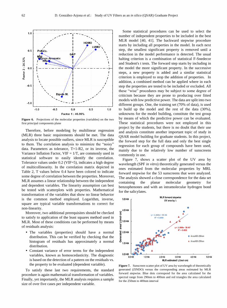
Figure 6 shows some molecular properties projected in the
plane corresponding to the two first principal components. It
is observed that the properties related to frontier orbitals and
the dipole moment are not grouped in the same quadrant. The
rest of molecular properties seem to have similar coordinates
(loadings), indicating their comparable contribution to the
factors. In view of this plot analysis, the molecular properties
that are not directly related with the electronic distribution
seem to provide nearly the same information, and they
should be treated as a single property.
Table 2. Correlation matrix for some selected molecular properties. Colored cells indicate a correlation higher than 0.6
ΔHf HOMO Dipo. Lamb. GAP #N #Rng LogP VC2 #ARng #2Bnd #O VC1 Polar. VC0 CI1 MW
ΔHf 1.0 -0.3 0.2 0.3 0.2 0.8 0.2 0.6 0.5 -0.5 -0.5 0.9 -0.7 0.5 -0.2 0.6 0.7
HOMO -0.3 1.0 -0.4 -0.4 0.3 -0.3 -0.4 -0.4 0.0 0.0 0.4 -0.3 -0.1 0.0 0.0 -0.4 -0.1
Dipole 0.2 -0.4 1.0 -0.1 -0.5 0.1 -0.1 0.3 0.2 -0.3 -0.1 0.1 -0.1 0.1 -0.3 0.3 0.2
Lambda 0.3 -0.4 -0.1 1.0 0.4 0.3 0.5 0.5 0.0 0.2 -0.4 0.5 0.0 0.0 0.2 0.4 0.0
GAP 0.2 0.3 -0.5 0.4 1.0 0.2 0.2 0.1 -0.1 0.3 -0.1 0.3 -0.1 0.3 0.3 -0.2 0.1
#N 0.8 -0.3 0.1 0.3 0.2 1.0 0.5 0.8 0.4 -0.6 -0.1 0.9 -0.3 0.4 0.1 0.6 0.3
#Ring 0.2 -0.4 -0.1 0.5 0.2 0.5 1.0 0.5 -0.4 0.0 -0.1 0.5 0.4 0.0 0.5 0.2 -0.3
Log P 0.6 -0.4 0.3 0.5 0.1 0.8 0.5 1.0 0.3 -0.5 -0.2 0.8 -0.2 0.1 0.0 0.6 0.2
VC2 0.5 0.0 0.2 0.0 -0.1 0.4 -0.4 0.3 1.0 -0.6 0.0 0.3 -0.9 0.3 -0.4 0.6 0.4
#ARing -0.5 0.0 -0.3 0.2 0.3 -0.6 0.0 -0.5 -0.6 1.0 -0.3 -0.5 0.4 -0.3 0.2 -0.5 -0.3
#2Bond -0.5 0.4 -0.1 -0.4 -0.1 -0.1 -0.1 -0.2 0.0 -0.3 1.0 -0.2 0.3 -0.1 0.4 -0.2 -0.7
#O 0.9 -0.3 0.1 0.5 0.3 0.9 0.5 0.8 0.3 -0.5 -0.2 1.0 -0.4 0.5 0.1 0.6 0.3
VC1 -0.7 -0.1 -0.1 0.0 -0.1 -0.3 0.4 -0.2 -0.9 0.4 0.3 -0.4 1.0 -0.4 0.4 -0.4 -0.7
Polariz 0.5 0.0 0.1 0.0 0.3 0.4 0.0 0.1 0.3 -0.3 -0.1 0.5 -0.4 1.0 -0.3 -0.1 0.4
VC0 -0.2 0.0 -0.3 0.2 0.3 0.1 0.5 0.0 -0.4 0.2 0.4 0.1 0.4 -0.3 1.0 0.0 -0.7
CI1 0.6 -0.4 0.3 0.4 -0.2 0.6 0.2 0.6 0.6 -0.5 -0.2 0.6 -0.4 -0.1 0.0 1.0 0.2
MW 0.7 -0.1 0.2 0.0 0.1 0.3 -0.3 0.2 0.4 -0.3 -0.7 0.3 -0.7 0.4 -0.7 0.2 1.0
62 D. González-Arjona et al.: Study of UV Filters as an in silico (QSAR) Graduate Project
Figure 6. Projections of the molecular properties (variables) on the two
first principal components plane
Therefore, before modeling by multilinear regression
(MLR) three basic requirements should be met. The data
analysis to locate possible outliers, since MLR is susceptible
to them. The correlation analysis to minimize the ―noisy‖
data. Parameters as tolerance, T=1-R2, or its inverse, the
Variance Inflation Factor, VIF = 1/T, are commonly used in
statistical software to easily identify the correlation.
Tolerance values under 0.2 (VIF=5), indicates a high degree
of multicollinearity. In the correlation matrix depicted in
Table 2, T values below 0.4 have been colored to indicate
some degree of correlation between the properties. Moreover,
MLR assumes a linear relationship between the independent
and dependent variables. The linearity assumption can best
be tested with scatterplots with properties. Mathematical
transformation of the variables that show no linear behavior
is the common method employed. Logarithm, inverse,
square are typical variable transformations to correct for
non-linearity.
Moreover, two additional prerequisites should be checked
to satisfy to application of the least squares method used in
MLR. Most of these conditions can be performed by means
of residuals analysis:
The variables (properties) should have a normal
distribution. This can be verified by checking that the
histogram of residuals has approximately a normal
distribution.
Constant variance of error terms for the independent
variables, known as homoscedasticity. The diagnostic
is based on the detection of a pattern on the residuals vs.
the property to be evaluated (dependent variable).
To satisfy these last two requirements, the standard
procedure is again mathematical transformation of variables.
Finally, yet importantly, the MLR analysis requires a sample
size of over five cases per independent variable.
Some statistical procedures can be used to select the
number of independent properties to be included in the best
MLR model [40, 41]. The backward stepwise procedure
starts by including all properties in the model. In each next
step, the smallest significant property is removed until a
reduction in the model performance is detected. The usual
halting criterion is a combination of statistical F-Snedecor
and Student's t tests. The forward step starts by including in
the model the more significant property. In the successive
steps, a new property is added and a similar statistical
criterion is employed to stop the addition of properties. In
addition, a combined method can be applied where in each
step the properties are tested to be included or excluded. All
these ―wise‖ procedures may be subject to some degree of
criticism because they are prone to producing over fitted
models with low predictive power. The data are split into two
different groups. One, the training set (70% of data), is used
to build up the model and the rest of the data (30%),
unknowns for the model building, constitute the test group
by means of which the predictive power can be evaluated.
These statistical procedures were not employed in this
project by the students, but there is no doubt that their use
and analysis constitute another important topic of study in
QSAR model building for graduate students. In this project,
the forward step for the full data and only the best single
regression for each group of compounds have been used,
mainly due to the relatively low number of sunscreens
commonly in use.
Figure 7, shows a scatter plot of the UV area by
wavelength (SPF in vitro) theoretically generated versus the
ones estimated from the molecular properties by MRL
forward stepwise for the 53 sunscreens that were analyzed.
The analysis showed a close correspondence for the data set
containing the planar molecular geometry for
benzophenones and with an intramolecular hydrogen bond
for the salicylates.
Figure 7. Sunscreen scatter plot of UV area by wavelength of theoretically
generated (ZINDO) versus the corresponding areas estimated by MLR
forward stepwise. Blue dots correspond for the area calculated for the
spectral range from 290nm to 400nm and red triangles the area calculated
for the 250nm to 400nm interval

Journal of Laboratory Chemical Education 2017, 5(4): 55-66 63
As was stated before, theoretical semi-empirical methods
employed (PM5 and INDO) tend to shift the absorption
peaks to shorter wavelength, into the UVC zone, if the
spectra are compared with those obtained experimentally in
nonpolar solvents. Thus, a lower sensitivity of the area under
the UVA and UVB zones is obtained. This is especially true
for the PM5 method, where the UV peaks are localized
below 280nm. Nevertheless, in order to compensate for this
theoretical spectral shift, the spectral area was also estimated
for a broader wavelength interval (250nm to 400nm) using
the ZINDO method. This area estimation provides larger
areas and therefore an increase in the sensitivity in the
variability among the compounds when part of the UVC
spectra is included in the generated area.
The relevant molecular properties that contribute
significantly to the MLR model, for the reduced wavelength
interval (290-400nm) are the total number of rings (#Rng),
the number of aromatic rings (#ARng), the dipole moment
(Dipole) and the HOMO/LUMO energy gap (GAP):
2 2
3 3(290-400nm)
2 4 5
Area/ 1.02 10 * ( Rng) 2.17 10 * ( ARng)
6.76 10 * (Dipole) 1.38 10 * (GAP) 1.03 10
RCV 0.839 0.890
# #
R
(7)
Figure 7 reveals a lack of significant differences, in terms
of correlation coefficient, when the wider UV interval is
employed. Nevertheless, except for variable HOMO/LUMO
energy gaps, the type of variables involved in the model
changes. Now, the number of nitrogen atoms, the valence
connectivity index 2, the heat of formation and the GAP are
significant:
(250 400 )
f
2 2
3 3
2 4
Area / 1.42 10 * (#N) 6.88 10 * (GAP)
3.62 10 * (VC 2) 58* ( H ) 5.64 10
RCV = 0.833 R = 0.853
nm
(8)
Thus, for the sake of simplicity, only the reduced
wavelength interval, (290nm-400nm) data set will be
analyzed.
When the whole data set is built up using the
benzophenones molecular group without necessarily
considering their planar molecular structure, slightly lower
regression coefficients (R2) are obtained (approx. 0.85), but
basically the same set of properties describe the MLR model:
number of all rings (#Rng), number of aromatic rings
(#ARng) and HOMO/LUMO energy gap (GAP).
When the entire data set is built up without considering the
possibility of intramolecular hydrogen bonding for the group
of salicylates, the regression coefficients decrease
significantly down to 0.6 if the same number of molecular
properties is included in the MLR model.
Table 3 collects a summary of the best single linear
regression analysis for the different groups of compounds.
There is no sense to apply the MLR model methodology to
each group of compounds considering the low number of
items in each group.
The correlation coefficient and RCV2 for salicylates group
without considering the intramolecular H bond is a
projection of the observed right spectra in Figure 4. The
spectral areas for the 290nm to 400nm interval are small and
very similar for the entire molecular group. Nevertheless,
this group of molecules with the intramolecular H bond
produces larger area values in the UVA spectral zone and
with some differences among the salicylates molecules.
These facts are reflected in better linear regression
parameters R2 and RCV2 obtained when considering the
intramolecular H bond.
Table 3. Best simple linear regression parameters for each molecular group
Compound group # items Property R2 RCV2
PABAs 5 GAP 0.832 0.632
Benzophenones (Planar) 12 GAP 0.941 0.853
Benzophenones 12 GAP 0.931 0.784
Camphors 6 GAP 0.912 0.802
Cinnamates 11 HOMO 0.843 0.800
Salicylates (H Bond) 6 #Double
bonds 0.908 0.747
Salicylates 6 Valence
Conn.2 0.486
No
variance
N-Heterocycles (Mix) 10 #ARing 0.566 0.510
On the other hand, the molecular property listed in Table 3
as having high significant linear correlation coefficients
seems to be different for the various molecular groups. Thus,
for p aminobenzoic acid, benzophenone and camphor
derivatives the HOMO/LUMO energy gap (GAP) is the
optimal molecular property that describes the linear
relationship. The best linear molecular property is not the
same one for rest of the molecular groups. A possible
explanation could be found if an extensive analysis of UV
spectra theoretically computed for each molecular group is
done. The position of the maximum wavelength and its
corresponding area for the HOMO/LUMO transition are
decisive in determining the contribution to the GAP
parameter. Thus, for benzophenones derivatives the
HOMO/LUMO transitions have maxima at wavelengths
over 340nm with a large extinction coefficient, so the GAP
parameter mainly contributes to the UV area. The salicylates
group also has maxima at wavelengths over 330nm, but their
extinction coefficients are approximately four times lower as
compared with the benzophenones group. Therefore, the
contribution to the UV area of the GAP parameter is lower.
Cinnamates derivatives have large extinction coefficients,
but the wavelengths at maxima are close to the UVB
limit (290nm). Finally, the N-heterocycles is a group of
compounds of a very different nature, (imidazole,
benzodiazole, triazin, …) with very diverse parameter values
for maximum wavelengths and extinction coefficients and
could be expected to have low linear correlation coefficients.
64 D. González-Arjona et al.: Study of UV Filters as an in silico (QSAR) Graduate Project
One step forward in the results analysis, not carried out by
the students in the project, is the Principal Component
Regression. This method combines the Principal Component
Analysis with MLR avoiding the multicollinearity issues.
PCR has been performed gradually using SPSS [40],
following the example reported by Liu et al. [49] Moreover,
none of the possible concerns expressed by Hadi and Ling in
[50] about their use are applicable in this study. In the first
step, the variables are statistically analyzed to fulfill the
MRL requirements and the correlated variables are dropped.
The factor analysis step indicates that seven principal
components are necessary to obtain nearly 100% of the
explained variance. This could be an indication that some
extra variables are needed in the model. The best model PCR
obtained provides a R2=0.883. The significant variables in
this model in order of their importance are, HOMO/LUMO
gap, wavelength with higher extinction coefficient, dipole
moment, number of molecular rings, number of double
bonds and number of oxygen atoms. Thus, a very similar
model is obtained with this more sophisticated procedure.
Finally, taken into account the undergraduate framework
in question, some remarks are in order regarding the present
study. The number of molecules has been limited to the
chemicals that have been internationally approved for use as
sun blockers. The undergraduate character of the project, as
well as time constraints, limited the level of quantum
calculations and the inclusion of solvent effects. Moreover, a
deeper analysis of the obtained area under the UV-Vis
(dependent variable) indicates that in some compounds there
are important contributions to this area by UV-Vis
transitions different from those associated with the
HOMO-LUMO gap. Thus, these facts will likely have a
negative impact on simple linear model building.
Notwithstanding these limitations, the various tools and
procedures used by the students in building the QSAR model
have provided a useful experience by showing them how
different tools and areas of chemistry can be combined to
obtain a near quantitative prediction of activities of
compounds from their chemical structure.
4. Conclusions
Modeling in silico UV-Vis spectra can be performed by
the configuration interaction singles (CI-s), a relatively
low-level computational method for computing excited
states. The project ambit, graduate level, simple organic
molecules, together with the possible computational
limitations, motivated the selection of a semi-empirical
theoretical method for molecular modeling.
Moreover, the UV-Vis spectrum is not influenced only by
the compound itself but also by its environment, such as the
solvent, solution pH, etc. These facts introduce some degree
of difficulty that have prevented QSAR studies from being
more widely used in chemical education.
Nevertheless, among the various semi-empirical methods,
ZINDO has parameters designed to match the UV-Vis
spectra. Despite the shift of the maxima in the case of some
spectra, the correct overall trend for the full UV-Vis spectra
of simple organic molecules can be obtained.
Additionally, the 2D-QSAR study is mainly concerned
with the correlation between the simple molecular structure
descriptors and the UV-Vis spectral area. Thus, in spite of
using approximate molecular modeling, the application of
this methodology has a reasonable basis. QSAR analysis
compares relative contributions and it is expected that the
method employed provides approximately the same shifts
for all molecules studied.
Therefore, this in silico QSAR study of sunscreens can be
a good starting point to introduce the QSAR methodology at
the final year undergraduate level. Nevertheless, limitations
of its applicability should be clearly pointed out.
ACKNOWLEDGEMENTS
The authors are very grateful to Prof. R. Rodríguez
Pappalardo for his helpful comments and suggestions. We
also thank to students of Chemistry: A. Martínez Pascual and
A. Palacios Morillo for their dedication in developing part of
the ―Sunscreen Project‖.
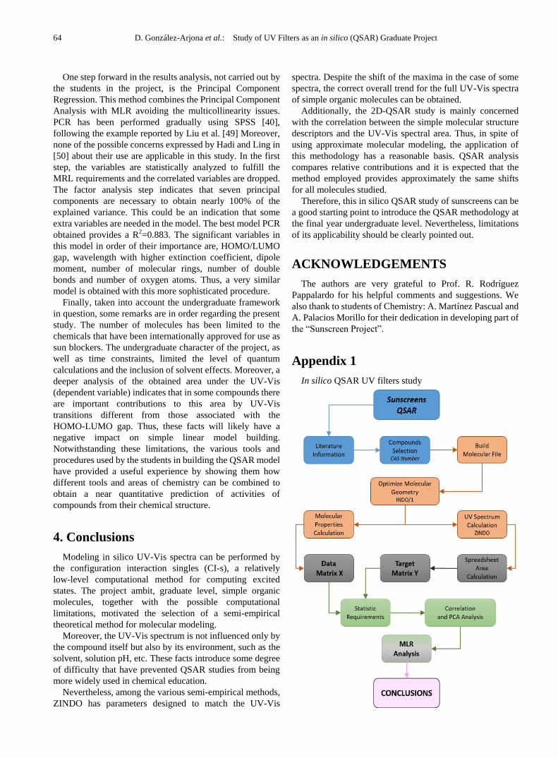
Appendix 1
In silico QSAR UV filters study

Journal of Laboratory Chemical Education 2017, 5(4): 55-66 65
QSAR topic selection (Blue section).
Update literature, SciFinder, Google scholar,…
Compounds collection, ref. 21 and literature cited
therein, FDA regulations,…
Unequivocally identification by CAS Registry
Number, ref 12.
Molecular modeling tool. CAChe, ref 42 (Orange section).
Molecular structure file generation.
From CAS registry #, the references 14 and 16 provide
an initial molecular file to be read by CAChe.
Ground state molecular geometry is optimized by
semi-empirical method INDO/1.
Estimation of molecular properties (Data matrix X),
using CAChe ProjectLeader. Export to Excel format.
UV spectra generation.
Generate UV spectrum using Configuration
Interaction, ref 22, and ZINDO, ref. 44.
Export a text file containing the UV-Vis spectrum at
1nm interval for each compound.
Spreadsheet calculations (Grey section).
Estimation of the UV area per unit of wavelength, eq. 1.
The integral is estimated by using the trapezoidal rule
(Target matrix Y).
Statistical calculations (Excel or statistical package,
references 40 and 41) (Green section).
Initial matrix data scrutiny: codification errors, outliers
values,…
Correlation matrix inspection, drop highly correlated
molecular properties.
Principal Component Analysis, projection of molecular
properties on factors space and estimation of maximum
number of variables.
Modeling strategy selection: Multi Linear Regression
(MLR).
Checking variable (molecular properties) for normal
distribution and homoscedasticity.
Molecular properties selection in the model by using
MRL forward stepwise.
Model cross-validation (not performed in this study).
Best simple linear regression for each class of organic
UV filter.
Conclusions (Pink section)
Advantages and disadvantages of QSAR.
REFERENCES
[1] Hansch, C., Maloney, P.P., Fujita, T. and Muir, R., Correlation of Biological Activity of Phenoxyacetic Acids with Hammett Substituent Constants and Partition Coefficients, 1962, Nature, 194, 178-180. doi:10.1038/194178b0.
[2] Food and Drug Administration (FDA). Critical Path Initiative. US Department of Health and Human Services, Rockville,
MD; 2010. https://www.fda.gov/ScienceResearch/SpecialTopics/CriticalPathInitiative/ucm204289.htm (Accessed March, 2017).
[3] European Chemicals Agency (ECHA), ―QSAR Toolbox‖, https://echa.europa.eu/support/oecd-qsar-toolbox (Accessed March, 2017).
[4] Shaath, N.A., On the theory of ultraviolet absorption by sunscreen chemicals, 1987, J. Soc. Cosmet. Chem., 82, 193-207.
[5] Agrapidis-Paloympis, L. E., Nash R.A. and Shaath N.A., The effect of solvents on the ultraviolet absorbance of sunscreens, 1987, J. Soc. Cosmet. Chem., 38, 209-221.
[6] Reichardt, C., Solvents and Solvent Effects: An introduction, 2007, Organic Process Research & Development, 11, 105–113.
[7] FDA, Sunscreen drug products for over-the-counter human use; final monograph, 2011. Federal Register 76/117, 35620-35665, USA. (Accessed March, 2017).
[8] Stiefel C. and Schwack W., Photoprotection in changing times – UV filter efficacy and safety, sensitization processes and regulatory aspects, 2015, Int. J. Cosmet. Sci., 37, 2–30.
[9] Dalby, A., Nourse, J. G., Hounshell, W. D., Gushurst, A. K. I., Grier, D. L., Leland, B. A. and Laufer, J., Description of several chemical structure file formats used by computer programs developed at Molecular Design Limited, 1992, Journal of Chemical Information and Modeling 32 (3), 244-255.
[10] National Computational Science Institute, ―Software Comparison Chart‖,http://www.computationalscience.org/ccce/about/whats_new/SoftwareComparison%20Lab1.pdf and http://www.computationalscience.org/ccce/about/whats_new/summary.pdf (Accessed March, 2017).
[11] Weininger D., SMILES, a chemical language and information system. 1. Intro-duction to methodology and encoding rules, 1988, Journal of Chemical Information and Modeling 28 (1), 31–6.
[12] CAS Registry. http://www.cas.org/content/chemical-substances (Accessed March, 2017)
[13] CACTUS. https://cactus.nci.nih.gov/chemical/structure. (Accessed March, 2017)
[14] ChemSpider. http://www.chemspider.com/Search.aspx. (Accessed March, 2017)
[15] ChemCell. https://github.com/cdd/chemcell. (Accessed March, 2017)
[16] Chemicalize. http://www.chemicalize.org/. (Accessed March, 2017).
[17] ACD/Labs. http://www.acdlabs.com/products/percepta/predictors.php (Accessed March, 2017).
[18] EPI Suite. https://www.epa.gov/tsca-screening-tools/epi-suitetm-estimation-program-interface. (Accessed March, 2017)
[19] ChemAxon. https://www.chemaxon.com/. (Accessed March, 2017).
[20] Mcule. https://mcule.com/. (Accessed March, 2017).

66 D. González-Arjona et al.: Study of UV Filters as an in silico (QSAR) Graduate Project
[21] González-Arjona, D., López-Pérez, G., Domínguez, M. M. and Cuesta van Looken, S., Study of Sunscreen Lotions, a Modular Chemistry Project, 2015, Journal of Lab-oratory Chemical Education, Vol. 3 No. 3, 44-52. doi:10.5923/j.jlce.20150303.02.
[22] J. B. Foresman and H. B. Schlegel, Application of the CI-Singles method in pre-dicting the energy, properties and reactivity of molecules in their excited states. Recent experimental and computational advances in molecular spectroscopy, Ed. R. Fausto and J. M. Hollas, Kluwer Academic: The Netherlands, 1993.
[23] Stephens, P. J. and Harada, N., ECD Cotton Effect Approximated by the Gaussian Curve and Other Methods, 2010, Chirality 22, 229-233.
[24] Plotting UV/Vis Spectra from Oscillator & Dipole Strengths, Gaussian Tech Notes, Feb 2016. http://gaussian.com/uvvisplot/ (Accessed March, 2017)
[25] Ridley, .J and Zerner, M., An intermediate neglect of differential overlap technique for spectroscopy: Pyrrole and the azines, 1973, Theor. Chim. Acta, 32, 111-134.
[26] Jacquemin D., Adamo C., Computational Molecular Electronic Spectroscopy with TD-DFT, Top Curr Chem. 2016; Vol. 368: 347-75. doi: 10.1007/128_2015_638.
[27] Lipinski C.A., Lombardo F., Dominy B.W. and Feeney P.J., ―Experimental and computational approaches to estimate solubility and permeability in drug discovery and development settings‖, Adv. Drug Deliv. Rev., 23, 3–25, (1997).
[28] Kamlet, M.J., Doherty, R.M., Abboud, J.L.M., Abraham, M.H. and Taft, R.W., Linear solvation energy relationships: 36. Molecular properties governing solubilities of organic nonelectrolytes in water, 1986, J. Pharmaceutical Sci. 75, 338-349.
[29] Mandloi M., Sikarwar A., Sapre NS., Karmarkar S. and Khadikar PV., A comparative QSAR study using Wiener, Szeged, and molecular connectivity indices, 2000, J. Chem. Inf. Comput. Sci., 40, 57-62.
[30] Gasteiger, J. and Marsili, M., Iterative partial equalization of orbital electronegativity—a rapid access to atomic charges, 1980, Tetrahedron, 36, 3219-3228.
[31] Stanton, D.T., Egolf, L.M., Jurs, P.C. and Hicks, M.G., Computer-assisted prediction of normal boiling points of pyrans and pyrroles, 1992, J. Chem. Inf. Comput. Sci., 32, 306-316.
[32] Sanniraghi, A.B., Ab initio Molecular Orbital Calculations of Bond Index and Valency, 1992, Adv. Quant. Chem., 23, 301-351.
[33] CODESSA Pro, http://www.codessa-pro.com/descriptors/ (Accessed March, 2017).
[34] Dragon 6, http://www.talete.mi.it/products/dragon_molecular_descriptors.htm (Accessed March, 2017)
[35] CORINA Symphony,https://www.mn-am.com/products/corinasymphony (Accessed March, 2017).
[36] Molecular Operating Environment, https://www.chemcomp.com/MOE-Molecular_Operating_Environment.htm (Accessed March, 2017).
[37] K. Varmuza and P. Filzmoser, Introduction to Multivariate Statistical Analysis in Chemometrics, Boca Raton, FL., CRC Press Taylor & Francis Group, 2009.
[38] A. Gustavo González, in Chemometrics in Practical Applications, K. Varmuza, (Ed.), 2012, InTech Pub., Rijeka, Croatia, pp 19-40.
[39] T.W. Anderson, An Introduction to Multivariate Statistical Analysis, 3rd Ed., pp. 291-458, John Wiley and Sons, New Jersey, 2003.
[40] SPSS Statistics, http://www-03.ibm.com/software/products/es/spss-statistics (Accessed March, 2017).
[41] Statsoft Statistica, https://www.statsoft.com/Products/STATISTICA-Features (Accessed March, 2017).
[42] Fujitsu CAChe Work System Pro 7.5.0.85, 2006, http://www.fqs.pl/chemistry_materials_life_science/products/scigress (Accessed March, 2017) and Teaching with CAChe: Molecular Modeling in Chemistry, C. Wong and J. Currie, Eds., 2002, New York, Fujitsu Limited.
[43] Miertus, S. and Tomasi, J., Approximate evaluations of the electrostatic free energy and internal energy changes in solution processes, 1982, Chem. Phys. 65, 239-245. doi:10.1016/0301-0104(82)85072-6.
[44] Zerner, M. C., Semiempirical Molecular Orbital Methods, in Reviews in Computational Chemistry, Volume 2 (Eds. K. B. Lipkowitz and D. B. Boyd), John Wiley & Sons, Inc., Hoboken, NJ, USA, 1991. doi: 10.1002/9780470125793.ch8.
[45] González-Arjona, D., López-Pérez, G., Domínguez, M. M. and González, A. G., Solvatochromism: A Comprehensive Project for the Final Year Undergraduate Chemistry Laboratory, 2016, J. Lab. Chem. Edu., 4(3), 45-52.
[46] Sugiyama, K., Tsuchiya, T., Kikuchi, A. and Yagi, M., Optical and electron paramagnetic resonance studies of the excited triplet states of UV-B absorbers: 2-ethylhexyl salicylate and homomenthyl salicylate, 2015, Photochem. Photobiol. Sci., 14, 1651-1659.
[47] Bos, J.D. and Meinardi, M.M., The 500 Dalton rule for the skin penetration of chemical compounds and drugs, 2000, Exp. Dermatol. 9, 165–169.
[48] Abdi H. and Williams, L.J., Principal component analysis, 2010, WIREs Comp. Stat. 2, 433-459. doi: 10.1002/wics.101.
[49] Liu, R.X., Kuang, J., Gong, Q. and Hou, X.L., Principal component regression analysis with SPSS, 2003, 71, 141-147.
[50] Hadi A.S. and Ling, R. F., Some Cautionary Notes on the Use of Principal Components Regression, 1998, American Statistician, 52, 15-19.


