Czech Technical University in Prague
Faculty of Electrical Engineering
Department of Control Engineering
Subspace Identification Methods
Technical Report
Ing. Pavel Trnka
Supervisor: Prof. Ing. Vladimır Havlena, CSc.
Prague, September 2005

Acknowledgement
First, I would like to thank to my supervisor Vladimır Havlena for his very good
guidance, his support and for sharing his ideas with me.
I would like to thank to my friends for letting me spend pleasant time with them
far away from the school and science, giving me new energy for my further work.
And finally I have to thank to my parents for their continuous support in anything
I do.
II

Abstract
This technical report shows the recent advances in Subspace Identification Methods
(4SID) and describes the reasons making these methods attractive to the industry.
The 4SID methods are used for the identification of the linear time-invariant models
in a state space form from the input/output data. On the contrary to the other
methods, they are based on the different principles, like the geometrical projections
and numerical linear algebra. Therefore the stress is laid on the interpretations
of these methods in the well known frameworks of Kalman filter, Prediction error
minimization and Instrumental variable methods. Recently proposed 4SID algo-
rithms, improvements and open problems are discussed and finally a new available
research direction in subspace identification is presented. The new idea would allow
to incorporate prior information into 4SID while recursifying the algorithm.
III
Contents
1 Introduction 1
1.1 Properties of 4SID methods . . . . . . . . . . . . . . . . . . . . . . . 1
2 Geometric Tools 4
2.1 Matrices with Hankel structure . . . . . . . . . . . . . . . . . . . . . 4
2.2 Matrix Row/Column Space . . . . . . . . . . . . . . . . . . . . . . . 5
2.3 Projections . . . . . . . . . . . . . . . . . . . . . . . . . . . . . . . . 5
2.4 Notes . . . . . . . . . . . . . . . . . . . . . . . . . . . . . . . . . . . . 8
3 Subspace Identification Methods 9
3.1 State Space Model . . . . . . . . . . . . . . . . . . . . . . . . . . . . 9
3.2 Notations and Definitions . . . . . . . . . . . . . . . . . . . . . . . . 10
3.3 Problem formulation . . . . . . . . . . . . . . . . . . . . . . . . . . . 12
3.4 Basic Idea . . . . . . . . . . . . . . . . . . . . . . . . . . . . . . . . . 13
3.5 Single equation formulation of SS model . . . . . . . . . . . . . . . . 14
3.6 Estimating subspaces . . . . . . . . . . . . . . . . . . . . . . . . . . 14
3.7 Estimating SS model parameters . . . . . . . . . . . . . . . . . . . . 18
3.8 N4SID algorithm summary . . . . . . . . . . . . . . . . . . . . . . . 20
3.9 Other 4SID algorithms . . . . . . . . . . . . . . . . . . . . . . . . . . 22
3.10 Historical note . . . . . . . . . . . . . . . . . . . . . . . . . . . . . . . 25
3.11 Notes . . . . . . . . . . . . . . . . . . . . . . . . . . . . . . . . . . . . 27
4 Interpretations and Relations 28
4.1 Multi-step Predictions Optimization . . . . . . . . . . . . . . . . . . 28
4.2 Kalman Filter Relation . . . . . . . . . . . . . . . . . . . . . . . . . . 33
4.3 Instrumental Variable Methods Relation . . . . . . . . . . . . . . . . 35
4.4 Notes . . . . . . . . . . . . . . . . . . . . . . . . . . . . . . . . . . . . 36
5 New Trends and Open Problems 37
5.1 Recursive 4SID . . . . . . . . . . . . . . . . . . . . . . . . . . . . . . 37
5.2 Closed-loop Identification . . . . . . . . . . . . . . . . . . . . . . . . 40
IV

6 Our Contribution and Future Research Direction 42
6.1 Our Contribution . . . . . . . . . . . . . . . . . . . . . . . . . . . . . 42
6.2 Prior knowledge incorporation . . . . . . . . . . . . . . . . . . . . . . 42
Abbreviations 45
References 48
My Publications 49
V


Chapter 1
Introduction
”The results of realization theory and the application of subspace identi-
fication algorithms form an example of what has been called the ‘unrea-
sonable effectiveness’ of mathematics.”
Jan H. van Schuppen, Vrije University, Amsterdam
Our research deals with relatively new methods in linear system identification, which
are generally entitled Subspace Identification Methods or more accurately 4SID
methods (Subspace State Space Systems IDentification). They are used for iden-
tification of LTI state space models directly from the input/output data. 4SID
methods are an alternative to the regression methods like ARX or ARMAX. How-
ever, they are based on a very different approach of the geometric projections and
linear algebra.
The basic ideas of these methods were developed about 20 years ago and they are
quite well accepted in the control engineering community, however the applications
of these methods in the systems identification are still rather exceptional, which
is mainly due to their complex theoretical backgrounds, until recently problematic
recursification and the problems with the closed-loop identification.
Up-to-date algorithms of 4SID methods are competing Prediction Error Methods
(PEM) in their performance and have shown several good properties, which make
them favorable candidate for the industrial applications.
1.1 Properties of 4SID methods
The following list shows the most important positive and negative properties of 4SID
methods.
Positive properties
MIMO systems identification. The complexity of the identification for large
MIMO (Multiple Inputs Multiple Outputs) systems is the same as for SISO
1

2 CHAPTER 1. INTRODUCTION
(Single Input Single Output) systems. There is no need for an extensive MIMO
structure parametrization, which is a very appealing property.
Numerical robustness. 4SID methods can be implemented with QR and SVD
factorizations, which have well known properties and very good numerical
robustness.
Few user parameters. In fact there is only one parameter and that is the system
order. There is no need for the complex parametrization even for MIMO
systems, because 4SID methods are identifying a state space model. Therefore
4SID methods are suitable for automatic multi-variable system identification.
Model order reduction. The algorithms of 4SID incorporates implicit model or-
der reduction, which is useful especially for the real-world data, where noises
and disturbances play important role and increase the order of estimated
model.
Negative properties
Need a large set of input/output data. The statistical properties of geometri-
cal methods used in 4SID are the reason for the fact, that they need large
amount of input/output data samples. That limits the application in some
areas, where data are rather rare, such as economic modelling.
Theoretically complex background. The algorithms are built on the geometri-
cal projections in the high dimensional row or column spaces of certain ma-
trices. This makes them uneasy to understand, however, as will be shown
(Chapter 4), they can be interpreted in the other well known frameworks.
Difficult recursification. The basic algorithms were developed to identify the sys-
tem parameters from off-line data, i.e. identification from given complete se-
quence of input/output data. However, the industrial applications need the
recursive algorithm to identify in the real-time from on-line data. This is still
rather problem for 4SID methods, but recent articles have shown promising
results.
Prior knowledge can not be easily incorporated into 4SID methods. These meth-
ods have black-box approach to the identified system, however there is often a
priori information, which should be exploited to increase the quality and the
robustness of the identification.
Recent articles showed, that subspace methods can be modified to perform well
even in the closed-loop identification [11, 12] and the new effective algorithms for
an on-line recursive identification [9, 10] were also proposed.

1.1. PROPERTIES OF 4SID METHODS 3
The usual description of a deterministic identification, which is rather academ-
ical, will be skipped in this work and the stochastic systems will be treated right
from the beginning.
This work is organized as follows. First an overview of the geometric tools, used
in 4SID, is presented in chapter 2. Chapter 3 shows the principles of 4SID methods
and describes the mostly used algorithms and their properties. Chapter 4 interprets
4SID methods in the well known frameworks of least-squares, Kalman filter and
instrumental variable methods. Chapter 5 summarizes the recent advances in the
field of 4SID, followed by chapter 6 proposing new research direction for our further
work, dealing with the prior information incorporation and 4SID recursification.
Several chapters are supplied with a section ’Notes’, usually giving the less formal
comments about the principles and the inner nature of the described methods.

Chapter 2
Geometric Tools
This chapter shows an overview of main geometric tools used in 4SID methods and
some necessary algebraic background. The main tools are the orthogonal and the
oblique projections.
2.1 Matrices with Hankel structure
The matrices with Hankel structure play important role in 4SID methods, because
the signals (the input/output data and the noises) appear in the algorithms in the
form of Hankel matrices. The first step of each algorithm is therefore to arrange the
available data into Hankel matrices.
A square or non-square matrix A ∈ Rm×n with Hankel structure is a matrix
with constant skew diagonals (anti-diagonals). In other words, in Hankel matrix,
the value of (i, j)th entry depends only on the sum i+ j. The matrix A with Hankel
structure can be created from a vector a =(
a1 . . . am+n−1
)with m + n − 1
elements
A =
a1 a2 a3 · · · an
a2 a3 a4 · · · an+1
a3 a4 a5 · · · an+2
......
.... . .
...
am am+1 am+2 · · · am+n−1
.
Each entry of Hankel matrix can be also a matrix. This composition is than called
Block Hankel matrix.
The matrices with Hankel structure are usually denoted shortly as Hankel ma-
trices, as it will be also used in this work. However, that can be confusing, because
Hankel matrix is also a special square matrix H ∈ Rn×n defined as
hi,j =
0 if i + j − 1 > n
i + j − 1 otherwise
4

2.2. MATRIX ROW/COLUMN SPACE 5
2.2 Matrix Row/Column Space
The row space of an m × n matrix A, denoted by row(A) is the set of all linear
combinations of the row vectors of A.
Similarly the column space of an m × n matrix A, denoted by col(A) is the set
of all linear combinations of the column vectors of A.
2.3 Projections
In this section the definitions of the orthogonal and the oblique projection will be
shown. General matrices A ∈ Rp×j, B ∈ Rq×j and C ∈ Rr×j will be considered.
Orthogonal Projection
The orthogonal projection of the row space A on the row space of B is defined as
A/B = ABT(BBT
)†B = AΠB, (2.1)
where •† is Moore-Penrose pseudo-inverse [14] of the matrix •. Similarly the pro-
jection of the row space A on the orthogonal space to the row space of B is defined
as
A/B⊥ = A (I − ΠB) = A(I −BT
(BBT
)†B
)= AΠ⊥
B, (2.2)
The projections A/B and A/B⊥ decompose the matrix A into two matrices,
whose row spaces are mutually orthogonal (Figure 2.1)
A = A/B + A/B⊥.
A/B⊥
B⊥
A/B B
A
Figure 2.1: Orthogonal projection.

6 CHAPTER 2. GEOMETRIC TOOLS
A numerically efficient and robust computation of the orthogonal projection can
be done by LQ decomposition1
(B
A
)= LQ =
(L11 0
L21 L22
)(Q1
Q2
).
Then, the the orthogonal projections can be written as
A/B = L21Q1, (2.3)
A/B⊥ = L22Q2. (2.4)
Oblique Projection
The oblique projection of the row space A along the row space of B on the row space
of C is defined as
A /B
C = A(CT BT
)[((
C
B
)(CT BT
))†]
first rcolumns
C. (2.5)
This result can be derived from an orthogonal projection of the row space A to the
row space of
(B
C
). A more effective way is to use LQ decomposition again
B
C
A
=
L11 0 0
L21 L22 0
L31 L32 L33
Q1
Q2
Q3
.
Then, the the orthogonal projections can be written as
A /B
C = L32L−122 C = L32L
−122
(L21 L22
) (Q1
Q2
). (2.6)
The oblique projection decomposes the matrix A into three matrices (Figure 2.2)
A = A /B
C + A /C
B + A/
(B
C
).
Statistical Properties of Projections
Assume two general sequences uk ∈ Rnu and ek ∈ Rne , k = 1, 2, . . . , j, where ek is
zero mean and independent of yk
E (ek) = 0,
E(uke
Tk
)= 0. (2.7)
1The LQ factorization of A is essentially the same as the QR factorization of AT . That isA = (AT )T = (QR)T = LQT

2.3. PROJECTIONS 7
A
B
CA /BC
A/CB A/
(BC)
Figure 2.2: Oblique projection.
For the long series of data (j → ∞) usual in 4SID and assuming ergodicity, the
expectation operator E can be replaced by an average over one, infinitely long
experiment
E(uke
Tk
)= lim
j→∞1
j
j∑i=1
uieTi . (2.8)
Putting the sequences into the row matrices
u =(
u1 u2 . . . uj
),
e =(
e1 e2 . . . ej
),
the sum in (2.8) can be rewritten to
E(uke
Tk
)= lim
j→∞1
jueT .
Considering independency (2.7) we find that
ueT = 0,
which implies that the signal u is perpendicular to the signal e.
Assume that y is a vector of the inputs and e is a vector of the additive distur-
bances. In the geometrical sense and for j →∞, the row vectors of the disturbances
are perpendicular to the row vectors of the inputs. Using an orthogonal projection
of the disturbance on the input, the noise is asymptotically eliminated
e/u = 0, (for j →∞).
This property is used in 4SID to eliminate the noise influence and is among basic
concepts of 4SID methods.

8 CHAPTER 2. GEOMETRIC TOOLS
2.4 Notes
The following notes may become more clear after reading the next chapter.
• An effect of the projections can be simplified into an ability to separate the
subspaces, which were joined together by a linear combination. The projec-
tions are able to eliminate the independent stochastic inputs, and to eliminate
the influence of measurable deterministic inputs.
• In the next chapter the deterministic inputs, disturbances and response from
the states will be shown to generate certain high-dimensional subspaces (spanned
by the rows of appropriate Hankel matrices). The output of LTI system will be
shown to generate similar subspace as a linear combination of these subspaces.
The power of projections is in their ability to separate this linear combination
from the knowledge of the inputs and outputs.
• The orthogonal projection is used to asymptotically eliminate the influence of
the disturbances from the joint space. This can be viewed as a separation of
an effective signal from the noise.
• The more capable oblique projection is also able to simultaneously eliminate
the influence of the disturbances and moreover to eliminate the influence of
the deterministic measurable signal (the input). This is mainly used in 4SID
methods to obtain the subspace generated only by the state sequence, which
is later used to obtain the model parameters.

Chapter 3
Subspace Identification Methods
Subspace identification methods are used to identify the parameters (matrices) of
LTI state space model from the input/output data. In this chapter the basics of
4SID methods will be given and three main algorithms (N4SID, MEOSP and CVA)
will be described.
The name ’subspace’ denotes the fact, that the model parameters of identified
linear system are obtained from the row or the column subspace of a certain matrix,
which is formed from the input/output data. Typically the column space is used to
extract information about the model and the row space is used to get Kalman filter
states sequence for the model.
3.1 State Space Model
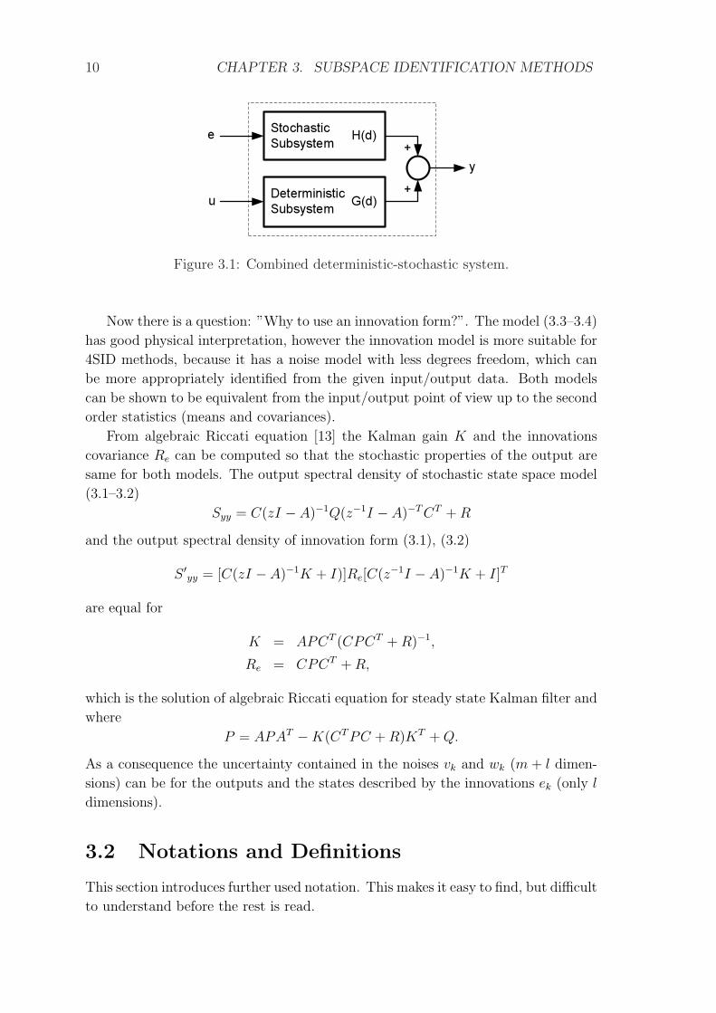
In this work we will consider a state space model of combined deterministic-stochastic
system (Figure 3.1) in an innovation form [7]
xk+1 = Axk + Buk + Kek, (3.1)
yk = Cxk + Duk + ek, (3.2)
where uk ∈ Rm is the m-dimensional input, xk ∈ Rn is the n-dimensional state,
yk ∈ Rl is the l-dimensional output, K is the steady state Kalman gain and ek ∈ Rl
is an unknown innovation with covariance matrix E[eke
Tk
]= Re. This model has
close relation with widely used stochastic state space model
xk+1 = Axk + Buk + vk, (3.3)
yk = Cxk + Duk + wk, (3.4)
where vk ∈ Rm and wk ∈ Rl are the process and the measurement noise with
covariance matrices E[vkv
Tk
]= Q, E
[wkw
Tk
]= R and E
[vkw
Tk
]= S. The process
noise represents the disturbances entering the system and the measurement noise
represent the uncertainty in the system observations.
9
10 CHAPTER 3. SUBSPACE IDENTIFICATION METHODS
StochasticSubsystem
DeterministicSubsystem
e
u
+
+y
H(d)
G(d)
Figure 3.1: Combined deterministic-stochastic system.
Now there is a question: ”Why to use an innovation form?”. The model (3.3–3.4)
has good physical interpretation, however the innovation model is more suitable for
4SID methods, because it has a noise model with less degrees freedom, which can
be more appropriately identified from the given input/output data. Both models
can be shown to be equivalent from the input/output point of view up to the second
order statistics (means and covariances).
From algebraic Riccati equation [13] the Kalman gain K and the innovations
covariance Re can be computed so that the stochastic properties of the output are
same for both models. The output spectral density of stochastic state space model
(3.1–3.2)
Syy = C(zI − A)−1Q(z−1I − A)−T CT + R
and the output spectral density of innovation form (3.1), (3.2)
S ′yy = [C(zI − A)−1K + I)]Re[C(z−1I − A)−1K + I]T
are equal for
K = APCT (CPCT + R)−1,
Re = CPCT + R,
which is the solution of algebraic Riccati equation for steady state Kalman filter and
where
P = APAT −K(CT PC + R)KT + Q.
As a consequence the uncertainty contained in the noises vk and wk (m + l dimen-
sions) can be for the outputs and the states described by the innovations ek (only l
dimensions).
3.2 Notations and Definitions
This section introduces further used notation. This makes it easy to find, but difficult
to understand before the rest is read.

3.2. NOTATIONS AND DEFINITIONS 11
One of the principaly new ideas in 4SID methods, is to combine the recursive
state space model into single linear matrix equation, relating the signal matrices
with the parameters matrices (Section 3.5). Prior to do this some definitions are
necessary.
Signal Related Matrices
For the use in 4SID algorithms, all signals (inputs, outputs and noises) are arranged
into the Hankel matrices. Assume known set of input/output data samples uk,yk for
k ∈ 〈0, 1, . . . , i + h + j − 2〉. These samples can be arranged into Hankel matrices
with i and h block rows and j columns as follows
(Up
Uf
)=
u0 u1 . . . uj−1
u1 u2 . . . uj
......
. . ....
ui−1 ui . . . ui+j−2
ui ui+1 . . . ui+j−1
ui+1 ui+2 . . . ui+j
......
. . ....
ui+h−1 ui+h . . . ui+h+j−2
=
(U+
p
U−f
)=
u0 u1 . . . uj−1
u1 u2 . . . uj
......
. . ....
ui−1 ui . . . ui+j−2
ui ui+1 . . . ui+j−1
ui+1 ui+2 . . . ui+j
......
. . ....
ui+h−1 ui+h . . . ui+h+j−2
,
where Up is the matrix of past inputs and Uf is the matrix of future inputs. Although
most data samples can be found in both matrices, the notation past/feature is
appropriate, because corresponding columns of Up and Uf are subsequent without
any common data samples and therefore have the meaning of the past and the future.
The distinction between the past and the future is important for Kalman filter and
Instrumental variables concepts used in 4SID.
Notice that the entries of Hankel matrices can be the vectors uk ∈ Rm, therefore
they are called block Hankel matrices with the dimensions Up ∈ Rim×j, Uf ∈ Rhm×j,
U+p ∈ R(i+1)m×j, U−
f ∈ R(h−1)m×j. The parameters i and h allow for the different
number of block rows for past Up and Uf future. This is different to some sources,
where both parameters are assumed equal.
The values of the coefficients i and h are usually selected slightly larger then the
upper bound of expected system order and the coefficient j is approximately equal
to the number of measured data at disposal (j À i, j À h). From i and h to j ratio
it is obvious that Hankel matrices Up and Uf have a structure with long rows.
Matrices U+p and U−
f are created from Up and Uf by moving the first block row
from Uf to the end of Up. This variation is later used to retrieve the system matrices.
For the outputs yk and the noises ek similar Hankel matrices Yp, Yf and Ep, Ef
can be constructed. A combination of Up and Yp denoted as Wp is used as a regressor
Wp =
(Up
Yp
)
12 CHAPTER 3. SUBSPACE IDENTIFICATION METHODS
System state sequence is also used in a matrix form with the following structure
Xp = (x0 x1 . . . xj−1) , Xf = (xi xi+1 . . . xi+j−1) .
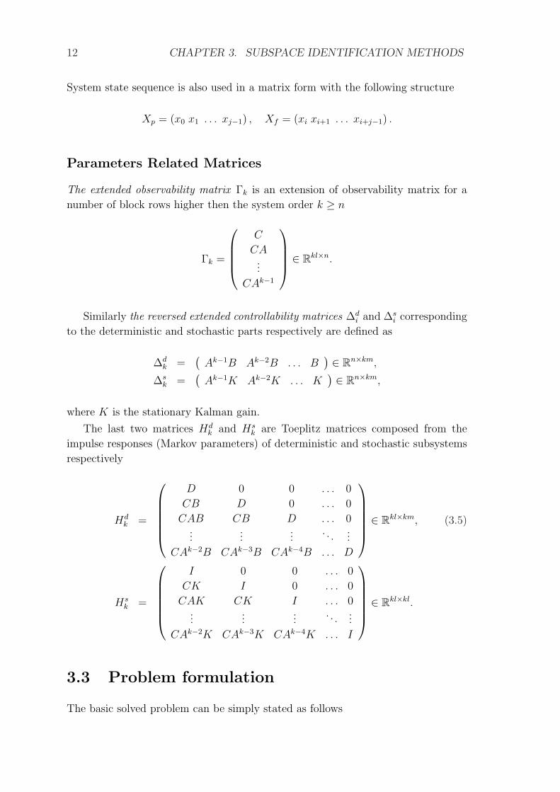
Parameters Related Matrices
The extended observability matrix Γk is an extension of observability matrix for a
number of block rows higher then the system order k ≥ n
Γk =
C
CA...
CAk−1
∈ Rkl×n.
Similarly the reversed extended controllability matrices ∆di and ∆s
i corresponding
to the deterministic and stochastic parts respectively are defined as
∆dk =
(Ak−1B Ak−2B . . . B
) ∈ Rn×km,
∆sk =
(Ak−1K Ak−2K . . . K
) ∈ Rn×km,
where K is the stationary Kalman gain.
The last two matrices Hdk and Hs
k are Toeplitz matrices composed from the
impulse responses (Markov parameters) of deterministic and stochastic subsystems
respectively
Hdk =
D 0 0 . . . 0
CB D 0 . . . 0
CAB CB D . . . 0...
......
. . ....
CAk−2B CAk−3B CAk−4B . . . D
∈ Rkl×km, (3.5)
Hsk =
I 0 0 . . . 0
CK I 0 . . . 0
CAK CK I . . . 0...
......
. . ....
CAk−2K CAk−3K CAk−4K . . . I
∈ Rkl×kl.
3.3 Problem formulation
The basic solved problem can be simply stated as follows
3.4. BASIC IDEA 13
Given
s samples of the input sequence u(0), . . . , u(s− 1) and the output
sequence y(0), . . . , y(s− 1)
Estimate
the parameters of the combined deterministic-stochastic model in the
innovation form (3.1–3.2). It means to estimate the system order n and to
obtain system matrices A, B, C, D, K and covariance matrix Re of the
noise ek.
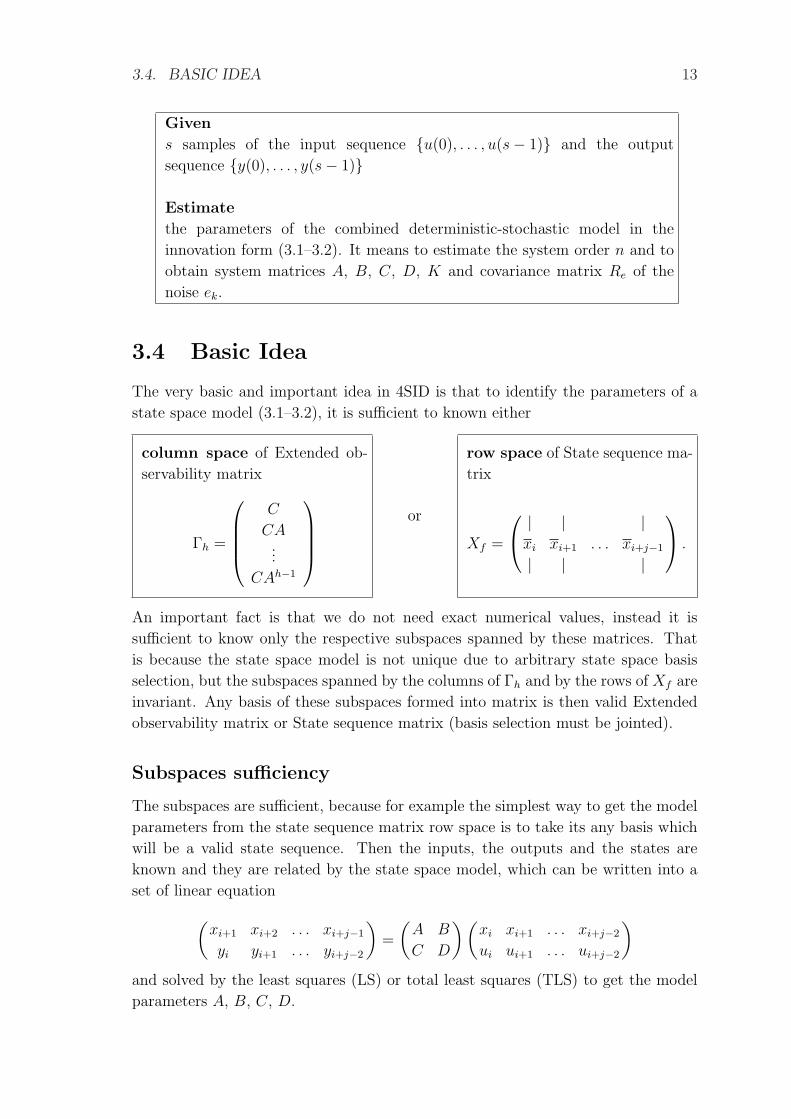
3.4 Basic Idea
The very basic and important idea in 4SID is that to identify the parameters of a
state space model (3.1–3.2), it is sufficient to known either
column space of Extended ob-
servability matrix
Γh =
C
CA...
CAh−1
or
row space of State sequence ma-
trix
Xf =
| | |xi xi+1 . . . xi+j−1
| | |
.
An important fact is that we do not need exact numerical values, instead it is
sufficient to know only the respective subspaces spanned by these matrices. That
is because the state space model is not unique due to arbitrary state space basis
selection, but the subspaces spanned by the columns of Γh and by the rows of Xf are
invariant. Any basis of these subspaces formed into matrix is then valid Extended
observability matrix or State sequence matrix (basis selection must be jointed).
Subspaces sufficiency
The subspaces are sufficient, because for example the simplest way to get the model
parameters from the state sequence matrix row space is to take its any basis which
will be a valid state sequence. Then the inputs, the outputs and the states are
known and they are related by the state space model, which can be written into a
set of linear equation
(xi+1 xi+2 . . . xi+j−1
yi yi+1 . . . yi+j−2
)=
(A B
C D
)(xi xi+1 . . . xi+j−2
ui ui+1 . . . ui+j−2
)
and solved by the least squares (LS) or total least squares (TLS) to get the model
parameters A, B, C, D.
14 CHAPTER 3. SUBSPACE IDENTIFICATION METHODS
3.5 Single equation formulation of SS model
As already mentioned before, the starting point of 4SID methods is a combination
of the recursive state space innovation model (3.1–3.2) into one single linear matrix
equation. This can be done with Hankel matrices by recursively substituting (3.1)
into (3.2)
Yp = ΓiXp + Hdi Up + Hs
i Ep, (3.6)
Yf = ΓhXf + HdhUf + Hs
hEf , (3.7)
Xf = AiXp + ∆di Up + ∆s
iEp. (3.8)
The equations (3.6) and (3.7) are similarly defining outputs as a linear combination
of previous states by the extended observability matrix Γ• (response from the states)
and a linear combination of previous inputs and noises by their respective impulse
responses Hd• and Hs
• . The equation (3.8) is relating the future and the past states
under the influence of the inputs and the noises.
3.6 Estimating subspaces
Assuming the sufficiency of the subspaces for SS model identification, now the prob-
lem of estimating invariant subspaces of the extended observability matrix Γh and
the state sequence matrix Xf from the input/output data will be treated. This
estimation is also related to the determination of the system order.
The important observation is that to obtain these subspaces, only the term ΓhXf
is needed and its estimate can be obtained from data by the projections. This term
is usually denoted as a matrix Oh
Oh = ΓhXf .
and it can be split into the required subspaces by singular value decomposition
(SVD).
Description of the matrix Oh content is usually avoided, but each column can
be seen as a response of the system to the nonzero initial state from an appropriate
column of the matrix Xf , without any deterministic or stochastic inputs.
The corollary is that Oh is numerically invariant to the changes of the state
space basis, although matrices Γh and Xf have invariant only the respective column
and row space.
Deterministic Oh splitting
For the pure deterministic system it is a simple task, because the matrix Oh has the
rank equal to the system order with the following SVD factorization
Oh = USV T =(
U1 U2
) (S1 0
0 0
)(V T
1
V T2
),
3.6. ESTIMATING SUBSPACES 15
where S1 is n× n sub-matrix of S containing nonzero singular values of Oh and U1
and V T1 are the appropriate parts of the matrices U and V T . The number of nonzero
singular values is equal to the order of the system and the required subspaces can
be obtained as
Γh = U1S1/21 , Xf = S
1/21 V T
1 ,
where a square root of S1 is simple, because S1 is a diagonal matrix. Notice that
multiplication by S1/21 can be omitted, because we are interested only in the spanned
spaces, but it is present for the equality Oh = ΓhXf to hold.
Stochastic Oh splitting
In the presence of the noise, the matrix Oh will be of the full rank. Thus all singular
values of Oh will be nonzero, i.e. the diagonal of the matrix S will have nonzero
entries in nonincreasing order. The rank of the identified system has to be chosen
from the number of significant singular values. This can be tricky task, for which few
theoretical guidelines are available. Assuming the system order to be determined,
the SVD matrices are partitioned into the ’signal’ and ’noise’ parts
Oh =(
Us Un
) (Ss 0
0 Sn
)(V T
s
V Tn
),
where Us and V Ts contain n principal singular vectors, whose corresponding singular
values are collected in the n× n diagonal matrix Ss. The ’cleaned’ estimates of the
extended observability matrix and state sequence matrix are then
Γh = UsS1/2s , Xf = S1/2
s V Ts . (3.9)
Estimating Oh from the I/O data
In this section the term ΓhXf will be obtained from the I/O data in the signal
matrices by an oblique projection. It will be obtained from the equation (3.7),
where the last two terms on the right side will be eliminated by a projection and
later it will be used as an approximation of Oh.= ΓhXf , where Xf is the Kalman
filter estimate of Xf from the available past data Wp.
Let’s try an orthogonal projection of the future output Yf onto the subspace of
past data Wp and future inputs Uf
Yf /
(Wp
Uf
)= Γh Xf + Hd
h Uf .
The orthogonal projection eliminated the noise term, because the estimated state
sequence Xf and the future inputs Uf lies in the joint row space of Wp and Uf ,
but the future noise Ef is perpendicular to this subspace for the number of samples
going to infinity (Figure 3.2).
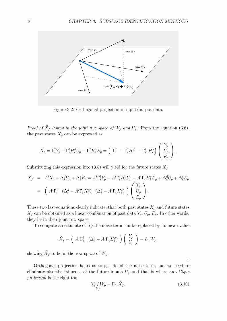
16 CHAPTER 3. SUBSPACE IDENTIFICATION METHODS
Figure 3.2: Orthogonal projection of input/output data.
Proof of Xf laying in the joint row space of Wp and Uf : From the equation (3.6),
the past states Xp can be expressed as
Xp = Γ†iYp − Γ†iHdi Up − Γ†iH
si Ep =
(Γ†i −Γ†iH
di −Γ†i Hs
i
)
Yp
Up
Ep
.
Substituting this expression into (3.8) will yield for the future states Xf
Xf = AiXp + ∆di Up + ∆s
iEp = AiΓ†iYp − AiΓ†iHdi Up − AiΓ†iH
si Ep + ∆d
i Up + ∆siEp
=(
AiΓ†i (∆di − AiΓ†iH
di ) (∆s
i − AiΓ†iHsi )
)
Yp
Up
Ep
.
These two last equations clearly indicate, that both past states Xp and future states
Xf can be obtained as a linear combination of past data Yp, Up, Ep. In other words,
they lie in their joint row space.
To compute an estimate of Xf the noise term can be replaced by its mean value
Xf =(
AiΓ†i (∆di − AiΓ†iH
di )
) (Yp
Up
)= LwWp,
showing Xf to lie in the row space of Wp.
¤Orthogonal projection helps us to get rid of the noise term, but we need to
eliminate also the influence of the future inputs Uf and that is where an oblique
projection is the right tool
Yf /Uf
Wp = Γh Xf . (3.10)
3.6. ESTIMATING SUBSPACES 17
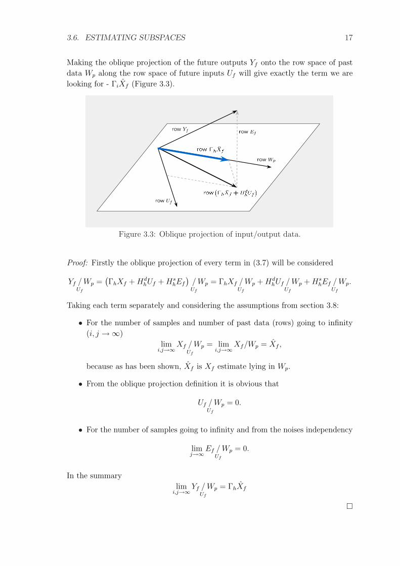
Making the oblique projection of the future outputs Yf onto the row space of past
data Wp along the row space of future inputs Uf will give exactly the term we are
looking for - ΓiXf (Figure 3.3).
Figure 3.3: Oblique projection of input/output data.
Proof: Firstly the oblique projection of every term in (3.7) will be considered
Yf /Uf
Wp =(ΓhXf + Hd
hUf + HshEf
)/Uf
Wp = ΓhXf /Uf
Wp + HdhUf /
Uf
Wp + HshEf /
Uf
Wp.
Taking each term separately and considering the assumptions from section 3.8:
• For the number of samples and number of past data (rows) going to infinity
(i, j →∞)
limi,j→∞
Xf /Uf
Wp = limi,j→∞
Xf/Wp = Xf ,
because as has been shown, Xf is Xf estimate lying in Wp.
• From the oblique projection definition it is obvious that
Uf /Uf
Wp = 0.
• For the number of samples going to infinity and from the noises independency
limj→∞
Ef /Uf
Wp = 0.
In the summary
limi,j→∞
Yf /Uf
Wp = ΓhXf
¤
18 CHAPTER 3. SUBSPACE IDENTIFICATION METHODS
All these projection equalities are exact for the number of data approaching
infinity (i, j →∞). To summarize the effect of the projections
Yf = Γh Xf + Hdh Uf + Hs
h Ef ,
Yf /
(Wp
Uf
)= Γh Xf + Hd
h Uf ,
Yf /Uf
Wp = Γh Xf .
3.7 Estimating SS model parameters
Assume that the matrix Oh is already known. Now it can be used to get the state
space model parameters by splitting it into the required subspaces by SVD as was
shown in the previous section. The parameters can be basically obtained from the
extended observability column space col(Γh) or the state sequence matrix row space
row(Xf ).
Estimating parameters from row(Xf)
Assume the inputs, the outputs and the state sequences are now available (the basis
for the state sequence row space was chosen)
Xi =(
xi, . . . , xi+j−1
), Xi+1 =
(xi+1, . . . , xi+j
),
Ui =(
ui, . . . , ui+j−1
), Yi =
(yi, . . . , yi+j−1
).
Then in the presence of no feedback the parameters of the innovation model can be
consistently estimated from the following matrix equation relating all data by the
state space model (Xi+1
Yi
)=
(A B
C D
) (Xi
Ui
)+ ε.
The solution can be obtained by least squares or total least squares. Denoting
Θ =
(A B
C D
), X =
(Xi
Ui
), Y =
(Xi+1
Yi
),
the least squares solution can be obtained as
Θ = YX † = YX T(XX T
)−1,
and the stochastic parameters as
Re = Σ22, K = Σ12Σ−122 ,
where
Σ =
(Σ11 Σ12
Σ21 Σ22
)=
1
j − (n + m)(Y −ΘX ) (Y −ΘX )T .
The consistency of solution requires j →∞.
3.7. ESTIMATING SS MODEL PARAMETERS 19
Estimating parameters from col(Γh)
First the extended observability matrix Γh is obtained as a basis of col(Γh) or it is
obtained directly from SVD of ΓhXf (3.9). Then the matrices A, B, C and D are
determined in two steps.
Determination of A and C
The matrix C can be read directly from the first block row of Γh. The matrix A is
determined from the shift structure of Γh. Denoting
Γh =
C...
CAk−2
∈ Rl(h−1)×n, Γh =
CA...
CAk−1
∈ Rl(h−1)×n,
where Γh is Γh without the last block row and Γh is Γh without the first block row,
the shift structure implies that
ΓhA = Γh.
This equation is linear in A and can be solved by LS or TLS.
Determination of B and D
Obtaining B and D is more laborious. Multiplying the I/O equation (3.7) from the
left by Γ⊥h and from the right by U †f yields to
Γ⊥h YfU†f = Γ⊥h ΓhXfU
†f + Γ⊥h Hd
hUfU†f + Γ⊥h Hs
hEfU†f ,
where Γ⊥h ∈ R(lh−n)×lh is a full row rank matrix satisfying Γ⊥h Γh = 0. The equation
can be simplified to
Γ⊥h YfU†f = Γ⊥h . Hd
h.
Denote i-th column of LHS as Mi and i-th column of Γ⊥h as Li, then
(M1 M2 . . . Mh
)=
(L1 L2 . . . Lh
)
D 0 0 · · · 0
CB D 0 · · · 0
CAB CB D · · · 0...
......
. . ....
CAh−2B CAh−3B CAh−4B · · · D
.
As shown in [1], this can be rewritten to
M1
M2
...
Mh
=
L1 L2 · · · Lh−1 Lh
L2 L3 · · · Lh 0
L3 L4 · · · 0 0...
.... . .
......
Lh 0 0 · · · 0
(Il 0
0 Γh
) (D
B
),
which is an overdetermined set of linear equations in the unknowns B and D and it
can be solved by LS or TLS.
20 CHAPTER 3. SUBSPACE IDENTIFICATION METHODS
3.8 N4SID algorithm summary
Here the complete 4SID algorithm [1] will be shown
Assumptions
1. The process noise wk and measurement noise vk are not correlated with the
input uk (open-loop identification).
2. The input u(t) is assumed to be persistently exciting [7] of the order i + h. It
means that the spectrum Θu(ω) is different from zero in at least i + h points
on the interval −π < ω < +π or that for multiple-input system the input
covariance matrix
Ruu =
(Up
Uf
)(Up
Uf
)T
has full rank which is m(i + h).
3. The number of measurements goes to infinity j →∞.
4. The user-defined weighting matrices W1 ∈ Rlh×lh and W2 ∈ Rj×j are such that
W1 is of full rank and W2 obeys: rank(Wp) = rank(WpW2).
Algorithm
1. Firstly arrange the I/O data into Hankel signal matrices Up, Uf , Yp, Yf and
their respective +/- modifications.
2. Calculate the oblique projections
Oh = Yf /Uf
Wp,
Oh+1 = Y −f /
U−f
W+p .
3. Compute SVD of the weighted oblique projection
W1OhW2 = USV T
4. Determine the system order by inspecting the singular values of S and partition
the SVD accordingly to obtain U1 and S1
Oh = USV T =(
U1 U2
) (S1 0
0 S2
)(V T
1
V T2
).

3.8. N4SID ALGORITHM SUMMARY 21
5. Determine Γh and Γh as
Γh = W−11 U1S
1/21 ,
Γh = Γh(1 : h− 1, :). (Matlab like notation)
6. Determine the state sequences
Xi = Γ†hOh,
Xi+1 = Γh†Oh+1.
7. Estimate the parameters A, B, C and D form a set of linear equations(
Xi+1
Yi
)=
(A B
C D
) (Xi
Ui
)+ ε.
8. Estimate the stochastic parameters Re and K from the covariance estimate of
the residuals as (Σ11 Σ12
Σ21 Σ22
)=
1
j − (n + m)εεT
Re = Σ22
K = Σ12Σ−122
There are several more sophisticated modification improving robustness and
eliminating bias.
Weighting matrices
The weighting matrices W1 and W2 were introduced to integrate several formerly
separate 4SID algorithms, which will be described later, into this single one [6].
W1 W2
N4SID Ili Ij
MOESP Ili Π⊥Uf
CVA((Yf/U
⊥f )(Yf/U
⊥f )T
)−1/2Π⊥
Uf
However there are some other interpretations of weighting matrices. 4SID meth-
ods determine Γh and Xf up to within a non-singular similarity transformation
T ∈ Rn×n
Γ′h = ΓhT
X ′f = T−1Xf .
This ambiguity raises the following question: In which state space basis are Γh
and Xf determined when a subspace method is used to estimate them? And that is
where the weighting matrices play the key role. The matrices W1 and W2 determines
the basis of estimates. By a proper choice of weighting matrices, the identification
result can be also influenced in a frequency specific way [7].
22 CHAPTER 3. SUBSPACE IDENTIFICATION METHODS
3.9 Other 4SID algorithms
The algorithm described in a previous section is called N4SID (Numerical algorithm
for 4SID) [1]. There are several others (PI-MOESP, PO-MOESP, CVA), which will
be described in this section. It is good to be aware, that all these advanced 4SID
algorithms share several fundamental steps. Early 4SID algorithms will be omitted,
because they work well for deterministic data, but struggle under the noise burden.
The idea is to correlate both sides of the basic matrix equation(3.11) with quantities
that eliminate the term with Uf and make the noise influence term with Ef disappear
asymptotically. In more details:
1. They all start with a single equation matrix formulation of SS model
Yf = ΓhXf + HdhUf︸ ︷︷ ︸
input term
+ HshEf︸ ︷︷ ︸
noise term
(3.11)
and try to use different projections to estimate the term ΓhXf out of Yf or at
least to get the column space of the extended observability matrix Γh. This
incorporates the elimination of the last two terms - the effect of the input and
the effect of the noise.
2. Removing the input term. The straightforward idea is to orthogonally
project (3.11) onto the row space orthogonal to Uf . The projection matrix
Π⊥Uf
= I − UTf
(UfU
Tf
)†Uf ,
will eliminate the input influence
UfΠ⊥Uf
= Uf − UfUTf
(UfU
Tf
)†Uf = 0,
but the noise term Ef will be left intact, because it is uncorrelated with the
deterministic input.
YfΠ⊥Uf
= ΓhXfΠ⊥Uf
+ Hsi EfΠ
⊥Uf
. (3.12)
The oblique projection used in N4SID combines this and the next step.
3. Removing the noise term. To eliminate the effect of the noise, the algo-
rithms use instrumental variable methods (IVM) with different instruments
selection. In some methods the IV principles are not obvious at the first sight
and will be discussed in Section 4.3.
Shortly it consists of finding good instruments ξ(t), which are uncorrelated
with the noise, sufficiently correlated with the state and which are orthogonal
to the inputs Uf . These instruments are usually created from the past inputs
and outputs Up, Yp to decorrelate the noise term from (3.12):
YfΠ⊥Uf
ξT = ΓhXfΠ⊥Uf
ξT ,
Hsi EfΠ
⊥Uf
ξT → 0 as j →∞.
3.9. OTHER 4SID ALGORITHMS 23
4. Finally they use the estimates of extended observable matrix Γh or state se-
quence matrix Xf or extended controllability matrix ∆h or their combination
to compute SS model parameters.
It is obvious, that there are several design variables in general 4SID algorithm,
which differentiate the particular algorithms. The reason for many 4SID algorithms
is the different selection of these design variables, because at present it is not
fully understood how to choose them optimally [7].
MOESP
The acronym MOESP [8, 16] stands for ”Multivariable Output Error State sPace”.
These methods are based on the combination of the projections and explicit instru-
mental variable methods. SS model parameters are recovered from the estimated
extended observability matrix.
For noise free data, the subspace identification reduces to the orthogonal projec-
tion of the equation (3.11) onto the row space of U⊥f , resulting in numerically exact
term ΓhXf . However in the presence of noise, the geometrical properties of (3.11)
are lost. Therefore the IVs are used as the instruments for removing the effect of the
noise term. The informative part of the signal term must, however, be left intact.
Let ξ(t) denote the vector of instruments. The instrumental variables must satisfy
the following requirements
1. IVs ξ(t) must be uncorrelated with the noise
E[e(t)ξ(t)T
]= 0.
2. IVs ξ(t) must be sufficiently correlated with the state to allow recovery of the
estimated Γh column space
rank(E
[x(t)ξ(t)T
])= n. (3.13)
3. IVs ξ(t) must be orthogonal to the input Uf (to leave the informative part
undisrupted).
The first two requirements (usual in IVM) suggest the input signal as a candidate
instrument. Clearly, this is incompatible with the third requirement. A solution
is the very partitioning of data into the past and the future parts. Afterwards the
feasible instrument is the past input Up.
For simultaneously removing the Uf term and decorrelating the noise, Verhaegen
[16] proposed to consider the following quantity (the equation 3.11 multiplied by
Π⊥Uf
UTp from the right side)
YfΠ⊥Uf
UTp = ΓhXfΠ
⊥Uf
UTp + Hs
hEfΠ⊥Uf
UTp . (3.14)
24 CHAPTER 3. SUBSPACE IDENTIFICATION METHODS
It is not difficult to see that the input term was eliminated Hdi UfΠ
⊥Uf
UTp = 0 and
the noise term is asymptotically disappearing with the number of samples going to
infinity
limj→∞
EfΠ⊥Uf
UTp = 0.
The rank condition (3.13) of the matrix
XfΠ⊥Uf
UTp
is shown in [16] to be equal to the number of purely deterministic states. In other
words, with only past inputs as IVs, only the deterministic subsystem can be iden-
tified. Any additional dynamics due to the colored disturbances are lost in the IVs
correlation. The algorithm based on this choice of IVs is called PI-MOESP (Past
Inputs MOESP) and it consists of applying SVD to LHS of (3.14) and taking its left
singular vectors as an estimate of the extended observability matrix, which is later
used for retrieving the system parameters.
If a complete state space model is desired, incorporating both the deterministic
and the stochastic subsystem, then IVs must be extended with the past outputs
Yp as an additional instrument. The algorithm is then called PO-MOESP (Past
Outputs MOESP). Similarly to (3.14) of PI-MOESP, with extended IVs we get
YfΠ⊥Uf
(UT
p
Y Tp
)= ΓhXfΠ
⊥Uf
(UT
p
Y Tp
)+ Hs
hEfΠ⊥Uf
(UT
p
Y Tp
). (3.15)
The matrix on the left side can be used as in PI-MOESP, but PO-MOESP usually
works differently. Firstly computing the following QR factorization
Uf
Up
Yp
Yf
=
L11 0 0 0
L21 L22 0 0
L31 L32 L33 0
L41 L42 L43 L44
Q,
where the Lii are lower triangular. The next step is to compute truncated SVD
(R42 R43
)= UsSsV
Ts + UnSnV
Tn .
The extended observability matrix is then estimated by Us, and A and C are ex-
tracted in the usual way. For finding B and D, Verhaegen argues [16] that the
least-squares solution to the overdetermined system of equations
(R31 R42
) ≈ Hdh
(R11 R22
)
provides a consistent estimate of Hdh, from which B and D are easily calculated.

3.10. HISTORICAL NOTE 25
CVA
CVA [22] is a class of algorithms, which stands for ”Canonical Variate Analysis”.
They are based on the concept of principal angles between subspaces.
The considered subspaces are the row space of conditional past data Wp/U⊥f
and the row space of conditional future outputs Yf/U⊥f . In [6] it is shown that
the number of principal angels between those subspaces[Wp/U
⊥f ^Yf/U
⊥f
]different
from π/2 is equal to the model order. Actually selecting non-perpendicular angles
for the noisy data is the same problem as selecting non-zero singular numbers of Oh
SVD in N4SID algorithm.
The fundamental idea of CVA is that the estimate of the future states Xf can be
found from the principal directions between past and future data[Wp/U⊥
f ^Yf/U⊥f
].
More precisely not the states, but their projection
[Wp/U⊥
f ^Yf/U⊥f
]= Xf/U
⊥f .
These methods, although they are based on the principal angles and directions, can
be also implemented by N4SID with appropriate weighting matrices (Section 3.8).
Larimore claims [22] that the weighting used for this method is optimal for the state
order determination from finite samples sizes. This has been shown by example, but
has never been proven. A last remark concerns the sensitivity to scaling. While the
algorithms N4SID and MOESP are sensitive to scaling of the inputs and/or out-
puts, the CVA algorithm is insensitive. This is because only angles and normalized
directions are considered in the CVA algorithm.
3.10 Historical note
The subspace methods have their origin in state-space realization theory as devel-
oped in the 1960s. A classical contribution is by Ho and Kalman (1966), where a
scheme for recovering the system matrices from the impulse response is outlined.
A problem with realization theory is the difficulty of obtaining a reliable non-
parametric estimate of the impulse response. A number of algorithms require special
inputs, such as impulse or white noise signals. An alternative approach is to extract
the desired information directly from the input/output data, without explicitly form-
ing impulse response and that is the case of 4SID methods.
Realization theory
Realization theory allows to get the system matrices of state space model from
a discrete impulse response of a system. Assume a state space description of a
deterministic system
x(t + 1) = Ax(t) + Bu(t), (3.16)
y(t) = Cx(t) + Du(t). (3.17)

26 CHAPTER 3. SUBSPACE IDENTIFICATION METHODS
This description is not unique due to arbitrary state space basis selection. For
any nonsingular matrix T ∈ Rn×n the state x(t) can be transformed to the new
state x(t) = T x(t) giving the following model
x(t + 1) = T−1ATx(t) + T−1Bu(t),
y(t) = CT x(t) + Du(t),
which is equivalent with (3.16),(3.17). However the impulse responses are the same
in any state space basis
H(z) = CT(zI − T−1AT
)−1T−1B + D = C (zI − A)−1 B + D = H(z)
The impulse sequence of the deterministic model can be easily computed from
(3.16–3.17) as
h(t) =
0 t < 0
D t = 0
CAt−1B t > 0
(3.18)
Consider the finite impulse sequence is known. The matrix D can be read directly
from h(0). To obtain other matrices the elements of impulse response are arranged
into Hankel matrix as follows
H =
h(1) h(2) h(3) . . . h(n + 1)
h(2) h(3) h(4) . . . h(n + 2)
h(3) h(4) h(5) . . . h(n + 2)...
.... . .
......
h(n + 1) h(n + 2) h(n + 3) . . . h(2n + 1)
.
Using (3.18) it is straightforward to verify that H can be factorized as
H = Γn+1∆n+1,
where
∆i =(
B AB . . . Ai−1B)
is the extended controllability matrix. For a minimal realization, the matrices Γn+1
and ∆n+1 have full rank, and hence H has rank n, equal to the system order. The
algorithm of Ho and Kalman is based on the above observations.
In the first step the matrix H is factorized by SVD to get Γn+1 and ∆n+1. In
the next step, the matrices B and C can be read directly from the first m columns
of ∆n+1 and l rows of Γn+1 respectively. The remaining matrix A is computed using
shift invariance structure of Γi:
Γn+1 = Γn+1A.
This property of extended observability matrix can be exploited by the use of least
squares or total least squares to get the system matrix A.
3.11. NOTES 27
The disadvantage of the realization methods is their need for the impulse re-
sponse. Several non-parametric methods can be used to estimate it, e.g. Correlation
analysis or Inverse discrete Fourier transformation, but the results are not satisfac-
tory. 4SID methods are in principal similar, but they do not need the impulse
response of the system.
The similarity is in the matrix Oh, which can be seen as ’an impulse response
from the states’. And it is shown to be equal to the multiplication of the extended
observability matrix and the state sequence matrix, just like H = Γn+1∆n+1. The
advantage is that Oh can be obtained directly from the I/O data.
3.11 Notes
• One has to keep in mind that 4SID consider signal matrices (Up, Uf , Yp, Yf ,
Ep, Ef ) as a definition of subspaces spanned by their rows. In other words the
exact numerical values of the row vectors are of lower importance.
• The very simple observation allowing us to work with the signal matrices row
spaces, is that in the single matrix SS equations (3.6-3.8), they are always
multiplied by the parameters matrices from the left. This means, that the
multiplication result and the result on the RHS is only a linear combination
of the signal matrix rows.
• The basic reasons allowing 4SID methods to work are simply non-uniqueness of
the state space model description and asymptotic properties of the projections
allowing to eliminate the noise and to project out the known input signal.
• Several proposed 4SID algorithms are basically same and they differ only in
the projection and instrumental variable selection and in the way of obtaining
the model parameters from the estimated subspaces of Γh or Xf . The N4SID
algorithm with the weighting matrices unifies the others, because its middle
product of the estimation, the matrix Oh, is independent of the state basis
selection.

Chapter 4
Interpretations and Relations
In this chapter, several interpretations of 4SID methods in the well known frame-
works will be shown in one integral form. The connections and the similarities with
other methods will be emphasized.
4.1 Multi-step Predictions Optimization
There is a natural question to ask about 4SID methods. Is there any criterion that is
minimized in the process of identification as it is usual for the other methods (ARX,
ARMAX)? Even the very recent articles [15] state, that there is no such suitable
minimization criterion:
”The available methods (4SID methods) are algebraic in nature as they
are not based on a suitable identification criterion minimization.”
However we have shown [21] that it is possible to find such criterion and by its
minimization, the pivotal oblique projection of N4SID can be obtained. In the
following, it will be shown, that 4SID methods are minimizing multi-step predictions
error of the model.
Multi-step Predictor Form
Assume the state space model (3.1–3.2) is known, and at time k, the system state
xk and the sequence of future inputs uk, uk+1, . . . , uk+h−1 are also known. Then
from the state equations (3.1–3.2) we can compute the predictions of the outputs
from 0 to h− 1 steps ahead (unknown innovations are replaced by their mean value
ek = 0)
yk+m =
Cxk + Duk m = 0,
CAmxk + Duk+m +m−1∑n=0
CAm−n−1Buk+n m ∈ 〈1, h− 1〉 .
28

4.1. MULTI-STEP PREDICTIONS OPTIMIZATION 29
This expression can be rewritten utilizing matrices defined in Section 3.2 as
yk
yk+1
...
yk+h−1
= Γhxk + Hd
h
uk
uk+1
...
uk+h−1
. (4.1)
In this way we get the sequence of output predictions from time k to k + h− 1 for
one initial time k. Additionally, the output predictions for j subsequent initial time
instants can be written in a compact form using Hankel matrix notation
yi . . . yi+j−1
yi+1 . . . yi+j
.... . .
...
yi+h−1 . . . yi+h+j−2
= Γh (xi . . . xi+j−1) + Hd
h
ui . . . ui+j−1
ui+1 . . . ui+j
.... . .
...
ui+h−1 . . . ui+h+j−2
,
which can be shortened to
Yf = ΓhXf + HdhUf . (4.2)
Note that every column of Yf represents the sequence of linear output predictions
(for the initial time determined by the index of the first element in the column) based
on the initial state x and the sequence of successive inputs u from the corresponding
columns.
An important property of the equation (4.2) is that for i, j → ∞ it can be
rewritten as
Yf = LwWp + HdhUf ,
where the future states Xf were replaced by a linear combination of past inputs
and outputs Wp =(
Yp
Up
)(as it was shown in Section 3.6). It correspond to the fact,
that the system states can be obtained from the Kalman filter running over infinite
set of historical input/output data Wp. System states are thus representing system
history.
In the real case, the condition i, j → ∞ is not satisfied (only a finite data set
is available) and thus the Kalman filter will give only the best possible linear state
estimate Xf based on available data. Then similarly like before it can be shown
that the following replacement can be made
Yf = ΓiXf + HdhUf ∼ Yf = LwWp + Hd
hUf , (4.3)
where Yf is the best output linear estimate using the limited available data set.
Estimated system states Xf are the same as we can obtain from the bank of
parallel non-stationary Kalman filters running over the columns of the matrix Wp
with the following initial conditions [1]
X0 = Xp /Uf
Up,
P0 = cov(Xp) =1
jXpX
Tp .
30 CHAPTER 4. INTERPRETATIONS AND RELATIONS
Deriving 4SID oblique projection from multi-step predictions
optimization
We will try to find a linear state space model of a certain order, that will most
accurately predict the behavior of the real process according to the measured data.
Firstly we will show how to derive the oblique projection (3.10) from the multi-step
predictor optimization and then we will reveal the intuition behind.
In other words we would like to find matrices Lw and Hi such that the predictions
according to the equation (4.3) will correspond with the measured data. The quality
of the predictions will be measured by Frobenius matrix norm
minLw,Hi
∥∥∥Yf − Yf
∥∥∥2
F= min
Lw,Hi
∥∥∥∥Yf −(
Lw Hi
) (Wp
Uf
)∥∥∥∥2
F
. (4.4)
Minimizing (4.4) means finding the best linear predictor in the sense of the least
squares. The optimal values of Lw and Hi can be found from matrix pseudo-inverse
(Lw Hi
)= Yf
(Wp
Uf
)†.
Denoting D =(
Wp
Uf
), the pseudo-inversion can be written as
(Lw Hi
)= YfDT
(DDT)−1
, (4.5)
multiplying both sides by the matrix D from the right yields to
(Lw Hi
)D︸ ︷︷ ︸Yf
= Yf DT(DDT
)−1D︸ ︷︷ ︸ΠD
. (4.6)
We obtained an expression
Yf = Yf
/(Wp
Uf
),
which represents the best linear prediction of Yf based on the available data. From
Yf we need to get only the part coming from the term LwWp, because it is equal to
ΓiXi, which is an estimate of the matrix Oi necessary for further identification using
SVD (Section 3.6). To get it separately from (4.6) it is sufficient to use the right
side of (4.5) and take only the first 2i columns and multiply them by the matrix Wp
alone
LwWp = YfDT[(DDT
)−1]first 2icolumns
Wp.
On the right side we obtained an expression for the oblique projection (2.5)
LwWp = Yf /Uf
Wp,

4.1. MULTI-STEP PREDICTIONS OPTIMIZATION 31
which can be rewritten using (4.3) as
Yf /Uf
Wp = ΓiXf (= Oi),
yielding to the fundamental equation of subspace identification algorithm (3.10).
If the following conditions are satisfied
• the deterministic inputs uk are not correlated with the stochastic inputs ek
(open-loop identification),
• the inputs uk and ek are persistently exciting (i.e. all modes of the system are
excited either by the inputs or by the noises),
• the number of measurements goes to infinity j →∞,
then the identification will be consistent.
ARMAX vs. 4SID
The interpretation showed in the previous section revealed that 4SID and ARMAX
have closer relation than it may seems on the first sight. Both can be interpreted
to identify the models, which are the optimal predictors, but with the different
optimality criterion.
Regression methods give a model, which is a single-step optimal predictor and
4SID methods give a model which is a multi-step optimal predictor.
ARMAX 4SID
minθ‖y − Zθ‖F min
∥∥∥Yf − Yf
∥∥∥F
= minLw,Hi
∥∥∥∥Yf −(
Lw Hi
) (Wp
Uf
)∥∥∥∥F
Consequences
• ARMAX is a single-step optimal predictor and it can be shown that by cyclic
application of this single-step optimal predictor we can get multi-step optimal
predictor.
• However, this is true, but only for the data generated by ideal linear system.
For the real-world data the multi-step predictions will not be optimal. And
that is where 4SIM comes. Their models give multi-step optimal predictions
even for the real-world data. Especially for the models with a reduced order
and for the colored noises.

32 CHAPTER 4. INTERPRETATIONS AND RELATIONS
Simulations
This section shows a comparison of the prediction abilities of ARMAX and 4SID
for non-ideal data and different model order reductions. The test input/output
sequences were generated by the 4th order state space model
xt+1 =
0.603 0.603 0 0
−0.603 0.603 0 0
0 0 −0.603 −0.603
0 0 0.603 −0.603
xt +
0.924
2.755
4.317
−2.644
ut +
−0.021
0.11
0.071
−0.103
et
yt =( −0.575 1.075 −0.523 0.183
)xt + (−0.714) ut + et
The quality of the models is estimated by the ability to predict, which is quite
different from the ability to accurately simulate the identified system, because for
predicting we need also a good description of the stochastic subsystem. Simulations
were done with 100 Monte-Carlo iterations using the following inputs:
Deterministic inputs: 1000 samples of Pseudo-Random Binary Signal (PRBS).
Stochastic inputs: white noise filtered with a low pass filter.
0 5 10 150
200
400
600
800
1000
1200
0 5 10 150
200
400
600
800
1000
1200
Prediction steps
4 →→→→ 2
4 →→→→ 3
4 →→→→ 4
4 →→→→ 2
4 →→→→ 3
4 →→→→ 4
0 5 10 150
200
400
600
800
1000
1200
Prediction steps
Su
m o
f pr
edic
tio
n er
ror
squa
res
4 →→→→ 44 →→→→ 34 →→→→ 2
ARMAX SIM
rank reduction
rank reduction
4 →→→→ 2
4 →→→→ 3
4 →→→→ 4
4 →→→→ 2
4 →→→→ 3
4 →→→→ 4
Figure 4.1: Prediction Error vs. Model Order.
Figure 4.1 shows two graphs relating the prediction error sum of squares to the
number of predictions steps for ARMAX and 4SID identification. Different line
colors represent different model order reductions and correspond for both graphs.
The blue lines represent identification without order reduction (not considerring
stochastic subsystem) and both methods give similar results. The green lines are
one order reduction from the 4th order to the 3rd order, where the difference is
4.2. KALMAN FILTER RELATION 33
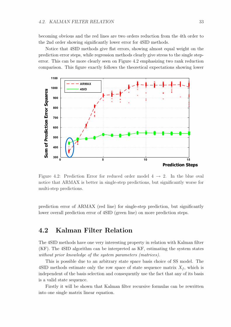
becoming obvious and the red lines are two orders reduction from the 4th order to
the 2nd order showing significantly lower error for 4SID methods.
Notice that 4SID methods give flat errors, showing almost equal weight on the
prediction error steps, while regression methods clearly give stress to the single step-
error. This can be more clearly seen on Figure 4.2 emphasizing two rank reduction
comparison. This figure exactly follows the theoretical expectations showing lower
0 5 10 15300
400
500
600
700
800
900
1000
1100
ARMAX4SID
Prediction Steps
Figure 4.2: Prediction Error for reduced order model 4 → 2. In the blue oval
notice that ARMAX is better in single-step predictions, but significantly worse for
multi-step predictions.
prediction error of ARMAX (red line) for single-step prediction, but significantly
lower overall prediction error of 4SID (green line) on more prediction steps.
4.2 Kalman Filter Relation
The 4SID methods have one very interesting property in relation with Kalman filter
(KF). The 4SID algorithm can be interpreted as KF, estimating the system states
without prior knowledge of the system parameters (matrices).
This is possible due to an arbitrary state space basis choice of SS model. The
4SID methods estimate only the row space of state sequence matrix Xf , which is
independent of the basis selection and consequently use the fact that any of its basis
is a valid state sequence.
Firstly it will be shown that Kalman filter recursive formulas can be rewritten
into one single matrix linear equation.
34 CHAPTER 4. INTERPRETATIONS AND RELATIONS
Non-steady state Kalman filter
Given:
• the initial state estimate x0,
• the initial estimate of the matrix P0,
• the input and output measurements u0, y0, . . . , uk−1, yk−1,
then the non-steady state Kalman filter state estimate xk is defined by the following
recursive formulas:
xk = Axk+1 + Buk + Kk−1 (yk−1 − Cxk−1 −Duk−1) , (4.7)
Kk−1 =(G− APk−1C
T) (
Λ0 − CPk−1CT)−1
, (4.8)
Pk = APk−1AT +
(G−APk−1C
T)(
Λ0− CPk−1CT)−1(
G−APk−1CT)T
,(4.9)
where G is state to output covariance matrix and Λ0 is the output covariance matrix,
defined as
G = AΣCT + S, Λ0 = CΣCT + R,
where Σ is the state covariance matrix E[xkx
Tk
]= Σ given by the solution of the
Lyapunov equation
Σ = AΣAT + Q.
In [1] it is shown and proved that the recursive KF formula (4.7 - 4.9) can be
rewritten into one single linear matrix equation as
xk =(
Ak − ΩkΓk ∆dk − ΩkH
dk Ωk
)
x0
u0
...
uk−1
y0
...
yk−1
,
where
Ωk =(∆c
k − AkP0ΓTk
) (Lk − ΓkP0Γ
Tk
)−1.
The significance of KF matrix form is that it indicates how the Kalman filter
state estimate xk can be written as a linear combination of the past input and output
measurements u0, y0, . . . , uk−1, yk−1.

4.3. INSTRUMENTAL VARIABLE METHODS RELATION 35
This allows the definition of the state sequence that is recovered by 4SID methods
with X0 as initial states
Xf =(
xi xi+1 . . . xi+j−1
)
=(
Ak − ΩiΓi ∆di − ΩiH
di Ωi
)
X0
Up
Yp
=(
Ak − ΩiΓi
(∆d
i − ΩiHdi Ωi
) ) (X0
Wp
). (4.10)
This state sequence is generated by a bank of non-steady state Kalman filters, work-
ing in parallel on each of the columns of the block Hankel matrix of past inputs and
outputs Wp. As can be seen, each state is filtered only from the limited length of
past input/output information (i samples), which is contained in one column of Wp.
Therefore the initial state estimate
X0 =(
x00 x0
1 x02 . . . x0
j−1
)
plays important role and advanced 4SID methods are shown to use nonzero initial
estimates. For example the described N4SID method uses
X0 = Xdp /
Uf
Up, (4.11)
where Xdp is the deterministic component of the state sequence matrix Xp.
One has to keep in mind, that this is only an interpretation of 4SID methods
from the Kalman filter point of view. For example the prior estimate (4.11) is
never computed in 4SID algorithm, but it can be shown that a bank of non-steady
state KF with this prior estimate and working with the input/output data from Wp
columns will give the same state sequence estimate as N4SID algorithm. The prior
estimate (4.11) can not be even explicitly computed, because for example Xdp is of
course a priori unknown.
The major observation in the subspace algorithms is that the system matrices
A, B, C, D, Q, R and S do not have to be known to determine the state sequence
Xf . It can be determined directly from the input/output data.
4.3 Instrumental Variable Methods Relation
Some 4SID methods can be interpreted to directly use the tools of Instrumental
variable methods (PI-MOESP, PO-MOESP), but in the others (N4SID, CVA), the
principles of IVMs are hidden. In this section, the methods will be compared from
IVMs point of view.
IVMs are traditionally used and well understood in PEM framework, the ex-
tension of IVMs to state space models is less obvious. It was shown in [8], that
36 CHAPTER 4. INTERPRETATIONS AND RELATIONS
subspace-based methods can be viewed as one way of generalizing IVMs in a nu-
merically reliable way for SS model identification.
The IVM approach in MOESP methods was described in Section 3.9. All meth-
ods are summarized in the following table:
Method Instrumental Variable Oh estimate
PI-MOESP Up YfΠ⊥Uf
PO-MOESP
(Up
Yp
)(Yf/Wp) Π⊥
Uf
N4SID
(Up
Yp
)Yf /
Uf
Wp
PO-MOESP and N4SID methods use identical instruments, but different weight-
ing matrices [8]. The resulting subspace estimates should therefore have very similar
properties. However, the schemes for unravelling the system matrices in MOESP
and 4SID are quite different.
Writing both estimate of Oh in the similar notation
ON4SID = YfΠ⊥Uf
W Tp (WpΠ
⊥Uf
W Tp )−1Wp,
OPO-MOESP = YfΠ⊥Uf
W Tp (WpΠ
⊥Uf
W Tp )−1WpΠ
⊥Uf
,
the difference is clear. It is only an extra projection Π⊥Uf
in PO-MOESP estimate.
4.4 Notes
As it has been illustrated in this chapter, 4SID methods are not so distant from the
traditional approaches, as it may seem at the first sight. They should be viewed
from two different view points:
1. As implicit implementation of Kalman filter. More precisely as a bank of
non stationary Kalman filters, estimating each state separately from i (chosen
parameter) historical I/O data and certain prior estimate. The important
property is that the system parameters (A,B,C,D,Q,R,S) are a priori unknown
and it is still possible to estimate systems states, but without particular basis
selection. This property of KF is less known.
2. Second view point is that by using 4SID methods for identification, we will get
the model with the optimal predictions for 1 to h (chosen parameter) steps.
More precisely the sum of squares for the sum of 1 to h predictions steps will
be minimal among all linear models of the same dimension. In other words,
4SID methods can be seen as a very elegant way how to specify and solve a
problem of identifying a model, which is optimal for multi-step predictions.
Chapter 5
New Trends and Open Problems
In this chapter some recent advances will be shown to complete the state-of-the-art
of 4SID. Nowadays, there are several open or only partially solved problems:
• Efficient recursive 4SID algorithm,
• Closed-loop identification,
• Prior knowledge incorporation,
• Optimal choice of the design variables for the general algorithm (weight ma-
trices W1, W2),
• Consistency, convergence and error analysis.
Here we will treat the first two problems, because their solution is in our industrially
motivated interest and several notable advances in these topics has been recently
made. The third problem of prior knowledge incorporation seems also to be very
interesting and in the next chapter, we will share some ideas, we have about our
further research in this direction.
5.1 Recursive 4SID
The main 4SID methods (N4SID, PI/PO-MOESP, CVA) are dedicated for identi-
fication from off-line data. Their good properties are appreciated, but for the real
industrial applications, especially in the control engineering, the efficient on-line re-
cursive identification algorithm is necessary. Great effort was recently devoted to
this field with many interesting results, but it seems that the goal is still far from
reached.
The off-line 4SID algorithms are directly unusable for on-line identification due
to the computationally burdensome steps such as singular value decomposition of
large matrices, which is the main bottleneck in recursification. Therefore it was
necessary to find SVD alternative algorithms in order to apply the subspace concept
in a recursive framework.
37
38 CHAPTER 5. NEW TRENDS AND OPEN PROBLEMS
The first attempts [18, 19], similarly compresses given I/O data recursively into
a matrix with a fixed size. An estimate of the extended observability matrix is not
updated directly, but in order to obtain the estimate, it is necessary to perform SVD
on the data-compressed matrix at every update step.
The recent advances [10, 9] took inspiration mainly from the methods used in
the field of Array Signal Processing, where a similar problem of Recursive Subspace
Tracking can be found and it is solved by Propagator method.
Recursive Subspace Tracking
A similar problem from the sensor array signal processing is following:
Assume we have an array with multiple antennas in configuration, where each
antenna has different directional sensitivity. The array is receiving several signals
as planar waveforms coming from the different directions (the distance between
antennas can be neglected). The considered problem is to recursively determine:
1. the number of incoming signals,
2. the direction of arrival for each signal,
3. reconstruct each waveform.
Mathematically the output from the general sensor array can be described as
follows
z(t) = Γ(θ)s(t) + b(t), (5.1)
where z is the output of nz sensors (antennas), s is the vector of ns signal waveforms
an b is the additive noise. The matrix Γ(θ) is the array propagation matrix. Each
column Γ(θ) =(
a(θ1) . . . a(θns))
represents the sensitivity of each sensor to the
respective waveform and it is a function of the direction of waveform arrival.
We can see that the problem 1 corresponds to the model order determination,
problem 2 is related to system modelling and problem 3 is Kalman filtering.
When studying the main techniques developed in both fields, it is interesting to
notice that the mathematical problem is the same: to track some eigencomponents
of particular matrices by adapting specific subspaces with the last observation. In
array signal processing, notable algorithms have been developed to avoid the use of
eigenvalue decomposition. Thus, it seems to be interesting to adapt some of these
SVD alternatives to recursive subspace identification.
The first step is to rewrite a state space model (3.1–3.2) into an equivalent form
to (5.1). Before it is necessary to introduce a temporal window
y+f (t) =
(yT (t) . . . yT (t + f − 1)
)T ∈ Rlf×1.
Then the state space model can be rewritten as
5.1. RECURSIVE 4SID 39
y+f (t) = Γfx(t) + Hd
f u+f (t) + Hs
fe+f (t)︸ ︷︷ ︸
=b+f (t)
.
The connection between subspace identification and array signal processing becomes
apparent by writing
z+f (t) = y+
f (t)−Hdf u+
f (t) = Γfx(t) + b+f (t).
The recursive algorithm is then made of two stages:
1. The update of the ”observation vector” z+f from the noisy input/output mea-
surements
z+f (t) = y+
f (t)−Hdf u+
f (t).
The matrix Hdf is unknown at time t since it is constructed from SS model
parameters. However, the observation vector z+f (t) can be obtained by the
projections.
2. The estimation of a basis of Γf from the observation vector
z+f (t) = Γfx(t) + b+
f (t). (5.2)
This step is carried out by Propagator method.
Propagator method
Assume that the system is observable. Then the extended observability matrix
Γ′f ∈ Rlf×n with lf > n, can be reorganized to Γf containing n linearly independent
vectors in the first rows, forming a submatrix Γf1 . Then, the complement Γf2 of Γf1
can be epxressed as a linear combination of this submatrix. So, there is a unique
linear operator Pf ∈ Rn×(fl−n) named propagator defined as
Γf2 = P Tf Γf2 .
It can be verified that
Γf =
(Γf1
Γf2
)=
(In
P Tf
)Γf1 .
Since rank(Γif
)= n
col (Γf ) = col
(In
P Tf
).
This last expression implies that it is possible to get an expression of the observability
matrix in a particular basis by determining the propagator. This operator can be
estimated from the equation (5.2). After having applied a data reorganization so

40 CHAPTER 5. NEW TRENDS AND OPEN PROBLEMS
that the first n rows of Γf are linearly independent, the following partition can be
introduced
z+f (t) =
(z+
f1(t)
z+f2
(t)
)=
(In
P Tf
)Γf1x(t) +
(b+f1
b+f2
).
In the noise free case it is easy to show that
z+f2
= P Tf z+
f1,
but in the presence of noise, the equality is lost. However, an estimate of P Tf can
be obtained by minimizing the following cost function
J(P Tf ) = E
∥∥z+f2− P T
f z+f1
∥∥2,
which leads to LS solution. Unfortunately this solution is biased even if the noise
is spatially and temporally white. Better solutions, circumventing this difficulty,
based on the correlations are proposed in [10].
Subspace prediction for time-varying systems
A new interesting 4SID algorithm for predicting linear time-varying systems has
been recently proposed in [9]. It uses a concept of principal angles [14] between
subspaces, spanned by the past and current extended observability matrix.
The future subspace is then predicted by rotating the current subspace in the
geometrical sense by the angles obtained from an extrapolation of the principal
angles development trend.
The proposed algorithm is recursive and it is suitable for identifying slowly time-
varying linear systems. Most existing systems show time-varying and/or nonlinear
behavior, and the nonlinear systems are sometimes treated as high order linear time-
varying systems from the practical point of view. Therefore this algorithm could be
used with an advantage for adaptive controllers or MPC.
5.2 Closed-loop Identification
The closed-loop identification is of special interest for a large number of engineer-
ing applications. For safety reasons or quality restrictions, it is desirable that the
identification experiments are carried out under the closed-loop conditions. The
fundamental problem with closed-loop data is the correlation between the unmea-
surable disturbances and the input caused by an effort of the controller to eliminate
the influence of disturbances [7].
It is well known, that the most traditional 4SID methods (N4SID, MOESP,
CVA) are not applicable to the systems operating under the closed-loop conditions
without special treatments [11]. Most of them can not provide consistent estimates
from the closed-loop I/O data.
5.2. CLOSED-LOOP IDENTIFICATION 41
However, the recent advances have shown that the modified 4SID algorithms can
work even under the closed-loop conditions [11, 12, 20]. The names of interested
people, such as Lennart Ljung show, that this research direction is promising. There
are recently two main approaches, which will be only sketched here:
Innovation Estimation Method (IEM) [20, 11] This method pre-estimates the
innovations e(t) and then use them as known, to decouple the noise and the
controlled input. The pre-estimation is usually done by a high order ARX or by
decomposing matrix equation (3.11) into i block rows, and use the estimated
innovations from the previous block rows to further estimate model parameters
of the next block row sequentially.
The basic idea is that under certain assumptions, the consistency estima-
tion with 4SID methods can be achieved if the innovation sequence is already
known.
Whitening Filter Approach (WFA) This approach claims not to require any ex-
tra data and not to be sensible to the instability in the deterministic subsystem
[12]. It is based on the idea of looking at the inverse system generating the
innovations e(t) from the joint process y(t) and u(t), namely the ”whitening
filter realization”
x(t + 1) = Ax(t) + Bu(t) + Ky(t),
e(t) = −Cx(t)−Du(y) + y(t),
where A = A − KC and B = B − KD. The state x(t) of this model is the
same as for the innovation model (3.1–3.2), therefore both models have the
same state space row(Xf ). The whitening filter can be rewritten into single
equation matrix form
Yf = ΓfXk + HfUf + GfYf + Ef .
The next difference to the standard algorithms is that the projections are car-
ried out on the model row by row (multi-stage projections). No pre-estimation
is involved, but the projections have to be done block-row wise to decouple
noise from control input.

Chapter 6
Our Contribution and Future
Research Direction
The reason of our interest in 4SID methods is their ability to identify large MIMO
systems without structural parametrization, their good numerical properties, and
because they also proved [23] to be beneficial in the industrially successful model
predictive control (MPC).
6.1 Our Contribution
So far, our main contribution to the field of Subspace identification was that 4SID
methods can be interpreted to identify the model as an optimal multi-step predictor
[21]. Our contribution is that we have mathematically derived that oblique projec-
tions used in Subspace identification can be obtained by minimizing the multi-step
prediction error criterium (4.4). Some results were shown in section 4.1. This also
showed 4SID methods in the well known framework of the least-squares and proved,
that even 4SID methods, with their geometrical identification approach, hide inside
a criterion, which is minimized during the identification process. As we have shown
this criterion was not expected to exist, as it was stated in some recent articles.
We are also very interested in the recursification, because it is an essential as-
sumption for the identification methods to be used in on-line industrial application.
Several algorithms have been proposed. The best one seems to be the subspace
tracking by propagator methods. Recusrification of 4SID would allow to create
adaptive MPC.
6.2 Prior knowledge incorporation
Our derivation of 4SID methods in the least-squares framework, showed new op-
portunity to incorporate prior knowledge, which is a persistent problem of 4SID
methods and as far as we know, no solution has been proposed yet.
42

6.2. PRIOR KNOWLEDGE INCORPORATION 43
To incorporate prior knowledge into the algorithm of 4SID identification would
be very beneficial. So far, 4SID methods have black-box approach to the identified
system. This is good for ’automatic identification’, where no additional information
about the identified system is available, but the I/O data may be corrupted and the
pure black-box approach may lead to a model, which is significantly deviated from
the real system.
However, there is often a priori information, which should be exploited to increase
the quality of the identification and to ensure that the identified model is close to
some expectations (lies within some boundaries). The following list shows some a
priori information, which would be useful to incorporated:
• known steady gain,
• known time constants range of step response,
• enforcing impulse (step) response smoothness - by specifying prior values of
impulse response second differences (useful to keep the model from fitting on
the high-frequency noise in data),
• Limit the step response to a funnel shaped region (Figure 6.1). This would
allow to constrain the time constants, model gain, over-shots and under-shots,
which would be very useful and versatile.
t
A
AmaxA0
0.9 A0
tmin tmax
Figure 6.1: A priory information as a funnel limiting model step response.
To incorporate prior information, we expect, that we will be able to minimize
the multi-step criterion
minLw,Hd
i
∥∥∥Yf − Yf
∥∥∥2
F= min
Lw,Hdi
∥∥∥∥Yf −(
Lw Hdi
) (Wp
Uf
)∥∥∥∥2
F
, (6.1)
while considering prior knowledge. This will involve to combine information from
the I/O measurements and a priori information, which can be done by covariance
matrix shaping and recursive least squares.
The expected main problems will be

44CHAPTER 6. OUR CONTRIBUTION AND FUTURE RESEARCH DIRECTION
1. The reformulation of some types of a priori information described above to
the prior information on the parameters, which are optimized in the multi-
step criterion (6.1), i.e. Lw and Hdi or maybe only on the matrix Oh. We hope
to take advantage of the fact, that these parameters are not dependent on the
state space basis selection, because they are related to the impulse responses
from the states and the inputs.
2. The recursification - we expect that the least squares approach would allow
straightforward recursification of 4SID algorithm. The stress would be on the
combination of the information from the input/output data and from a priori
information on the model which have to be combined in each step.
The preliminary idea of the complete recursive algorithm is following:
1. Transformation of a priori information about the identified system to the co-
variance matrices of Lw and Hdi , which are minimized in the criterion (and
maybe to their prior mean values).
2. Recursive least squares minimization of (6.1) while combining the information
from the previous step with the new information from the measured data and
a priori information. Some type of forgetting should be incorporated, but we
have to assure that a priori information about the system is not completely
forgotten. Usual recursive minimization is possible, because the equation
Yf =(
Lw Hdi
) (Wp
Uf
)+ ε,
is linear in the parameters Lw and Hdi , and the sizes of Lw and Hd
i are inde-
pendent on the amount of measured data.
3. Finally Lw can be used to estimate the system order and to estimate sys-
tem matrices A and C, because it has the same column space as extended
observability matrix Γi, since
LwWp = ΓiXf .
This fact should be exploited by SVD or Propagator method. Matrices B and
D can be for example obtained from Hdi .
Note that the matrix Hdi , with the deterministic impulse response in the Toeplitz
form, has lower triangular form (3.5). Obtaining Hdi with large nonzero entries above
the main diagonal means badly conditioned I/O data.

Abbreviations
4SID Subspace State Space System Identification
ARX Auto-Regressive with eXogenous inputs
ARMAX Auto-Regressive Moving Average with eXogenous inputs
CVA Canonical Variate Analysis
IV Instrumental Variable
LTI Linear Time Invariant
LS Least Squares
IEM Innovation Estimation Method
IVM Instrumental Variable Methods
KF Kalman Filter
LHS Left Hand Side
MOESP Multivariable Output Error State sPace
MPC Model Predictive Control
N4SID Numerical Subspace State Space System Identification
PEM Prediction Error Methods
PI-MOESP Past Inputs Multivariable Output Error State sPace
PO-MOESP Past Outputs Multivariable Output Error State sPace
RHS Right Hand Side
SS State Space
TLS Total Least Squares
WFA Whitening Filter Approach
45

Bibliography
[1] Peter Van Overschee and Bart De Moor. Subspace Identification for Linear
Systems: Theory-Implementation-Applications. Kluwer Academic Publishers,
1996.
[2] Hiroshi Oku and Hidenori Kimura. Recursive 4SID algorithms using gradient
type subspace tracking. Automatica, 38:1035–1043, June 2002.
[3] Wouter Favoreel, Bart De Moor, and Peter Van Overschee. Subspace state
space system identification for industrial processes. Journal of Process Control,
10:149–155, 2000.
[4] Anders Lindquist and Giorgio Picci. Geometric Methods for State Space Iden-
tification (unpublished).
[5] W. Favoreel, B. De Moor, M. Gevers, and P. Van Overschee. Closed loop
model-free subspace-based LQG-design (unpublished). 1998.
[6] Peter Van Overschee and Bart De Moor. A Unifying Theorem for Three Sub-
space System Identification. Automatica, Special Issue on Trends in System
Identification, 31(12):1853–1864, 1995.
[7] Lennart Ljung. System Identification: Theory for the User (2nd Edition). Pren-
tice Hall PTR, 1998.
[8] Mats Viberg. Subspace-based Methods for the Identification of Linear Time-
invariant Systems. Automatica, 31(12):1835–1851, 1995.
[9] Kentaro Kameyama and Akira Ohsumi. Recursive Subspace Prediction of Lin-
ear Time-Vayring Stochasti Systems. In Proceedings of the 16th IFAC World
Congress. Kidlington, Oxford, GB, Elsevier, 2005. ISBN 0-08-144130-1.
[10] Guillaume Mercere, Stephane Lecæuche, and Christian Vasseur. Sequential
Correlation Based Propagator Algorithm for Recursive Subspace Identification.
In Proceedings of the 16th IFAC World Congress. Kidlington, Oxford, GB,
Elsevier, 2005. ISBN 0-08-144130-1.
46
BIBLIOGRAPHY 47
[11] Weilu Lin, S. Joe Qin, and Lennart Ljung. Comparison of Subspace Identifi-
action Methods for Systems Operating on Closed-loop. In Proceedings of the
16th IFAC World Congress. Kidlington, Oxford, GB, Elsevier, 2005. ISBN
0-08-144130-1.
[12] Alessandro Chiuso and Giorgio Picci. Prediction Error vs. Subspace Methods
in Closed Loop Identification. In Proceedings of the 16th IFAC World Congress.
Kidlington, Oxford, GB, Elsevier, 2005. ISBN 0-08-144130-1.
[13] Mohinder S. Grewal and Angus P. Andrews. Kalman Filtering: Theory and
Practise, Second Edition. John Wiley & Sons, 2001. ISBN 0-471-39254-5.
[14] David A. Harville. Matrix Algebra From a Statistician’s Perspective. Springer,
1997. ISBN 038794978X.
[15] Pouliquen Mathieu and M’Saad Mohammed. An Interpretation of Subspace
Identification Methods. In Proceedings of the 16th IFAC World Congress.
Kidlington, Oxford, GB, Elsevier, 2005. ISBN 0-08-144130-1.
[16] M. Verhaegen. Identification of the deterministic part of MIMO state space
models given in innovations form from input-output data. Automatica, 30:61–
74, 1994.
[17] Peter Van Overschee and Bart DeMoor. N4SID: Subspace Algorithms for
the Identification of Combined Deterministic-Stochasti Systems. Automatica,
30:75–93, 1994.
[18] Hiroshi Oku and Hidenori Kimura. A Recursive 4SID from the Input-Output
Point of View. Asian Journal of Control, 1(4):258–269, 1999.
[19] Y. M. Cho, G. Xu, and T. Kailath. Fast Recursive Identification of State Space
Models via Exploitation of Dispalcement Structure. Automatica, 30(1):45–59,
1994.
[20] Weilu Lin, S. Joe Qin, and Lennart Ljung. A Framework for Closed-loop Sub-
space Identification with Innovation Estimation. Technical Report 2004-07,
Texas-Wisconsin Modeling and Control Consorcium, February 2004.
[21] Pavel Trnka and Valdimır Havlena. Subspace Identification as Multi-step Pre-
dictions Optimization. In Proceedings of the Fifth IASTED International Con-
ference on Modelling, Simulation and Optimization, pages 223–228. Anaheim:
ACTA Press, 2005. ISBN: 0-88986-524-8.
[22] W. E. Larimore. Canonical variate analysis in identification, filtering and adap-
tive control. In Proceedings of 29th Conference on Decision and Control, Hawai,
USA, pages 596–604, 1990.

48 BIBLIOGRAPHY
[23] Ramesh Kadali, Biao Huang, and Anthony Rossiter. A Data Driven Sub-
space Approach to Predictive Controller Design. Control Engineering Practise,
11:261–278, 2002.
My Publications
[1] Pavel Trnka and Petr Smolık. Profibus DP Master for PC. In Proceedings of
8th International Student Conference on Electrical Engineering POSTER 2004
[CD-ROM]. Prague: CTU FEE Prague, 2004.
[2] Jirı Roubal, Vladimır Havlena, Jaroslav Neuhauser, and Pavel Trnka. MPC Con-
troller for Two-Dimensional Systems. In Proceedings of the 15th International
Conference on Systems Science, pages 132–140. Wroclaw: Oficyna Wydawnicza
Politechniki Wroclawskiej, 2004. ISBN 83-7085-804-X.
[3] Jirı Roubal, Vladimır Havlena, and Pavel Trnka. Simulation of Two-Dimensional
Distributed Parameters Systems. In Proceedings of Matlab 2004 Conference,
volume 1-2, pages 500–504. Prague: Institute of Chemical Technology, 2004.
ISBN 80-7080-550-1.
[4] Pavel Trnka and Hana Pytelova. Czech Economy Model Estimation by the
Bootstrap Filter. In Proceedings of 9th International Student Conference on
Electrical Engineering POSTER 2005 [CD-ROM]. Prague: CTU FEE Prague,
2005.
[5] Pavel Trnka, Vladimır Havlena, and Jan Stecha. Bootstrap Filtering for Czech
Macro-economic Model Estimation. In Proceedings of 15th International Con-
ference on Process Control 05 [CD-ROM]. Bratislava: Slovak University of Tech-
nology, 2005. ISBN 80-227-2235-9.
[6] Pavel Trnka and Valdimır Havlena. Subspace Identification as Multi-step Pre-
dictions Optimization. In Proceedings of the Fifth IASTED International Con-
ference on Modelling, Simulation and Optimization, pages 223–228. Anaheim:
ACTA Press, 2005. ISBN: 0-88986-524-8.
49


![Visual Attention Framework: Application to Event Analysishomepages.inf.ed.ac.uk/rbf/CVonline/LOCAL_COPIES/... · and Selective Attention for Identiflcation Model (SAIM) [20]. A formal](https://cdn.vdocument.in/doc/165x107/5f2ade966d7e5a40d671f90c/visual-attention-framework-application-to-event-and-selective-attention-for-identiication.jpg)


