
Supervised Learning Decision Trees
Road Map
1. Basic Concepts of Classification
2. Decision Tree Induction
3. Attribute Selection Measures
4. Pruning Strategies

Definition
¤ Supervised Learning is also called Classification (or Prediction)
¤ Principle ¤ Construct models (functions) based on training data
¤ The training data are labeled data
¤ New data (unlabeled) are classified using the training data
Model
Class label
Numeric value Unlabeled data
Age Income 29 25K
[Budget Spender]
[Budget Spender (0.8)]
Age Income Class label
27 28K Budget-Spenders
35 36K Big-Spenders
65 45K Budget-Spenders
Training data

Classification vs Prediction
¤ Classification predicts categorical class labels (discrete or nominal)
¤ Prediction models continuous-valued functions, i.e., predicts unknown or missing values (ordered values)
¤ Regression analysis is used for prediction
Customer profile
Classifier Budget Spender
Numeric Prediction 150 Euro
Customer profile

Entropy: Bits
http://www.cs.cmu.edu/~guestrin/Class/10701-S06/Handouts/recitations/recitation-decision_trees-adaboost-02-09-2006.ppt
¤ You are watching a set of independent random samples of X
¤ X has 4 possible values: A, B, C, and D
¤ The probabilities of generating each value are given by:
P(X=A)=1/4, P(X=B)=1/4, P(X=C)=1/4, P(X=D)=1/4
¤ You get a string of symbols ACBABBCDADDC…
¤ To transmit the data over binary link you can encode each symbol with bits (A=00, B=01, C=10, D=11)

Entropy: Bits
http://www.cs.cmu.edu/~guestrin/Class/10701-S06/Handouts/recitations/recitation-decision_trees-adaboost-02-09-2006.ppt
¤ Now someone tells you the probabilities are not equal
P(X=A)=1/2, P(X=B)=1/4, P(X=C)=1/8, P(X=D)=1/8
¤ In this case, it is possible to find coding that uses only 1.75 bits on the average
¤ E.g., Huffman coding
¤ Compute the average number of bits needed per symbol

Entropy: General Case
http://www.cs.cmu.edu/~guestrin/Class/10701-S06/Handouts/recitations/recitation-decision_trees-adaboost-02-09-2006.ppt
¤ Suppose X takes n values, V1, V2,… Vn, and
P(X=V1)=p1, P(X=V2)=p2, … P(X=Vn)=pn
¤ The smallest number of bits, on average, per symbol, needed to transmit the symbols drawn from distribution of X is given by:
¤ H(X) = the entropy of X
)(log)( 21
i
m
ii ppXH ∑
=
−=
Entropy Definition
http://www.cs.cmu.edu/~guestrin/Class/10701-S06/Handouts/recitations/recitation-decision_trees-adaboost-02-09-2006.ppt
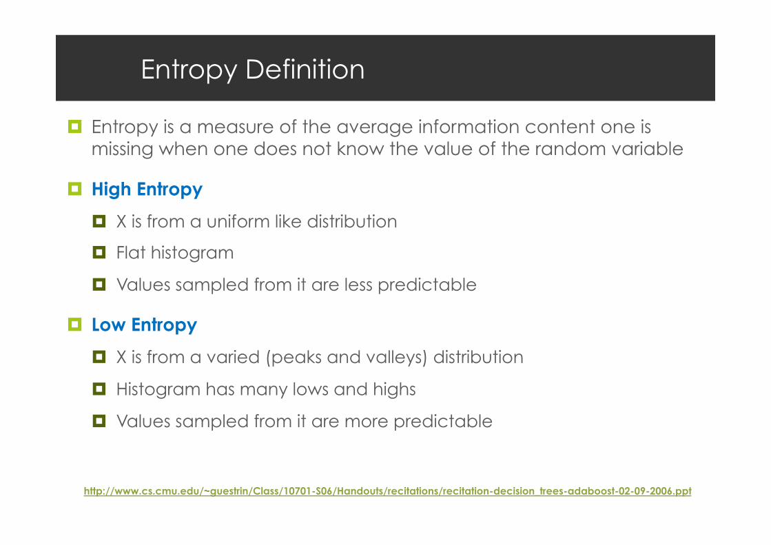
¤ Entropy is a measure of the average information content one is missing when one does not know the value of the random variable
¤ High Entropy
¤ X is from a uniform like distribution
¤ Flat histogram
¤ Values sampled from it are less predictable
¤ Low Entropy
¤ X is from a varied (peaks and valleys) distribution
¤ Histogram has many lows and highs
¤ Values sampled from it are more predictable

Road Map
1. Basic Concepts of Classification
2. Decision Tree Induction
3. Attribute Selection Measures
4. Pruning Strategies
Decision Tree Induction
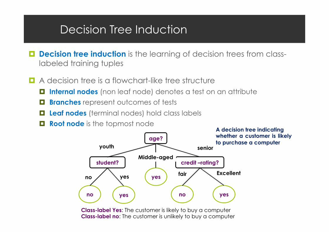
¤ Decision tree induction is the learning of decision trees from class-labeled training tuples
¤ A decision tree is a flowchart-like tree structure ¤ Internal nodes (non leaf node) denotes a test on an attribute
¤ Branches represent outcomes of tests
¤ Leaf nodes (terminal nodes) hold class labels
¤ Root node is the topmost node
age?
student? credit –rating?
no yes yes no
yes
youth
Middle-aged
senior
yes no fair Excellent
A decision tree indicating whether a customer is likely to purchase a computer
Class-label Yes: The customer is likely to buy a computer Class-label no: The customer is unlikely to buy a computer

Decision Tree Induction
¤ How are decision trees used for classification? ¤ The attributes of a tuple are tested against the decision tree
¤ A path is traced from the root to a leaf node which holds the prediction for that tuple
¤ Example
¤ Test on age: youth
¤ Test of student: no
¤ Reach leaf node
¤ Class NO: the customer
Is unlikely to buy a
computer
age?
student? credit –rating?
no yes yes no
yes
youth
Middle-aged senior
yes no fair Excellent
A decision tree indicating whether a customer is likely to purchase a computer
RID age income student credit-rating Class 1 youth high no fair ?

Decision Tree Induction
¤ Why decision trees classifiers are so popular? ¤ The construction of a decision tree does not require any domain
knowledge or parameter setting ¤ They can handle high dimensional data ¤ Intuitive representation that is easily understood by humans ¤ Learning and classification are simple and fast ¤ They have a good accuracy
¤ Note ¤ Decision trees may perform Differently depending on the data set
¤ Applications ¤ Medicine, astronomy ¤ Financial analysis, manufacturing ¤ Many other applications
age?
student? credit –rating?
no yes yes no
yes
youth
Middle-aged
senior
yes no fair Excellent
A decision tree indicating whether a customer is likely to purchase a computer

The Algorithm
Principle ¤ Basic algorithm (adopted by ID3, C4.5 and CART): a greedy algorithm
¤ Tree is constructed in a top-down recursive divide-and-conquer manner
¤ Iterations
¤ At start, all the training tuples are at the root
¤ Tuples are partitioned recursively based on selected attributes
¤ Test attributes are selected on the basis of a heuristic or statistical measure (e.g., information gain)
¤ Stopping conditions
¤ All samples for a given node belong to the same class
¤ There are no remaining attributes for further partitioning – majority voting is employed for classifying the leaf
¤ There are no samples left

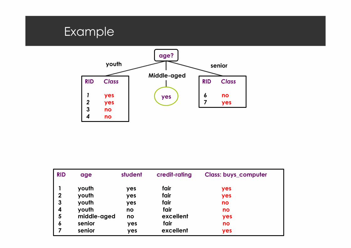
Example
age? youth
Middle-aged
senior
RID Class 1 yes 2 yes 3 no 4 no
RID Class 5 yes
RID Class 6 no 7 yes
RID age student credit-rating Class: buys_computer 1 youth yes fair yes 2 youth yes fair yes 3 youth yes fair no 4 youth no fair no 5 middle-aged no excellent yes 6 senior yes fair no 7 senior yes excellent yes
Example
age? youth
Middle-aged
senior
RID Class 1 yes 2 yes 3 no 4 no
RID Class 6 no 7 yes
RID age student credit-rating Class: buys_computer 1 youth yes fair yes 2 youth yes fair yes 3 youth yes fair no 4 youth no fair no 5 middle-aged no excellent yes 6 senior yes fair no 7 senior yes excellent yes
yes

Example
age? youth
Middle-aged
senior
RID Class 4 no
RID Class 6 no 7 yes
student?
yes no yes
RID Class 1 yes 2 yes 3 no
RID age student credit-rating Class: buys_computer 1 youth yes fair yes 2 youth yes fair yes 3 youth yes fair no 4 youth no fair no 5 middle-aged no excellent yes 6 senior yes fair no 7 senior yes excellent yes

Example
age? youth
Middle-aged
senior
RID Class 6 no 7 yes
student?
yes no yes
RID Class 1 yes 2 yes 3 no
no
Majority voting
RID age student credit-rating Class: buys_computer 1 youth yes fair yes 2 youth yes fair yes 3 youth yes fair no 4 youth no fair no 5 middle-aged no excellent yes 6 senior yes fair no 7 senior yes excellent yes

Example
age? youth
Middle-aged
senior
RID Class 6 no 7 yes
student?
yes no yes
no
RID age student credit-rating Class: buys_computer 1 youth yes fair yes 2 youth yes fair yes 3 youth yes fair no 4 youth no fair no 5 middle-aged no excellent yes 6 senior yes fair no 7 senior yes excellent yes
yes

Example
age? youth
Middle-aged
senior
RID Class 7 yes
student?
yes no yes
no yes
RID age student credit-rating Class: buys_computer 1 youth yes fair yes 2 youth yes fair yes 3 youth yes fair no 4 youth no fair no 5 middle-aged no excellent yes 6 senior yes fair no 7 senior yes excellent yes
credit –rating?
fair Excellent
RID Class 6 no

Example
age? youth
Middle-aged
senior
student?
yes no yes
no yes
RID age student credit-rating Class: buys_computer 1 youth yes fair yes 2 youth yes fair yes 3 youth yes fair no 4 youth no fair no 5 middle-aged no excellent yes 6 senior yes fair yes 7 senior yes excellent no
credit –rating?
fair Excellent
yes no

Three Possible Partition Scenarios
Partitioning scenarios
Examples
A?
a1 a2
…av
Discrete-valued
Continuous-valued
Discrete-valued+ binary tree
A?
A<=split-point A>split-point
A∈SA
yes no
Color?
red green bleu pink
orange
income?
low medium high
income?
<=42,000 >42,000
Color ∈{red, green}
yes no

Road Map
1. Basic Concepts of Classification
2. Decision Tree Induction
3. Attribute Selection Measures
4. Pruning Strategies

Attribute Selection Measures
¤ An attribute selection measure is a heuristic for selecting the splitting criterion that “best” separates a given data partition D
Ideally ¤ Each resulting partition would be pure ¤ A pure partition is a partition containing tuples that all belong to the same
class
¤ Attribute selection measures (splitting rules) ¤ Determine how the tuples at a given node are to be split ¤ Provide ranking for each attribute describing the tuples ¤ The attribute with highest score is chosen ¤ Determine a split point or a splitting subset
¤ Methods ¤ Information gain ¤ Gain ratio ¤ Gini Index

Quiz
¤ In both pictures A and B the child is eating a soup
¤ Which situation (A or B) has a high/low entropy in terms of the locations of the soup?
From: http://www.autonlab.org/tutorials/infogain11.pdf
A B
The values (locations of
the soup) sampled
entirely from within the soup ball The values (locations of the soup)
almost unpredictable…almost uniformly sampled throughout the living room
High Entropy Low Entropy

Information Gain Approach
¤ D: the current partition
¤ N: represent the tuples of partition D
¤ Select the attribute with the highest information gain (based on the work by Shannon on information theory)
¤ This attribute ¤ minimizes the information needed to classify the tuples in the resulting
partitions ¤ reflects the least randomness or “impurity” in these partitions
¤ Information gain approach minimizes the expected number of tests needed to classify a given tuple and guarantee a simple tree
First Step
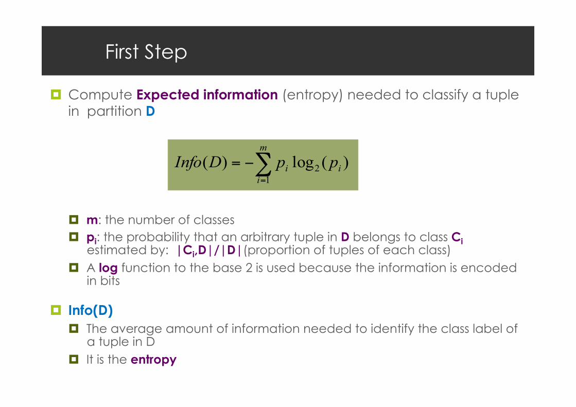
¤ Compute Expected information (entropy) needed to classify a tuple in partition D
¤ m: the number of classes ¤ pi: the probability that an arbitrary tuple in D belongs to class Ci
estimated by: |Ci,D|/|D|(proportion of tuples of each class) ¤ A log function to the base 2 is used because the information is encoded
in bits
¤ Info(D) ¤ The average amount of information needed to identify the class label of
a tuple in D ¤ It is the entropy
)(log)( 21
i
m
ii ppDInfo ∑
=
−=

Example
m=2 (the number of classes) 9 tuples in class yes N= 14 (number of tuples) 5 tuples in class no
RID age income student credit-rating class:buy_computer 1 youth high no fair no 2 youth high no excellent no 3 middle-aged high no fair yes 4 senior medium no fair yes 5 senior low yes fair yes 6 senior low yes excellent no 7 middle-aged low yes excellent yes 8 youth medium no fair no 9 youth low yes fair yes 10 senior medium yes fair yes 11 youth medium yes excellent yes 12 middle-aged medium no excellent yes 13 middle-aged high yes fair yes 14 senior medium no excellent no
bits 940.0)145(log
145)
149(log
149)( 22 =−−=DInfo
In partition D

Second Step
¤ For each attribute, compute the amount of information needed to arrive at an exact classification after portioning using that attribute
¤ Suppose that we were to partition the tuples in D on some attribute A {a1…,av} ¤ Split D into v partitions {D1,D2,…Dv} ¤ Ideally Di partitions are pure but it is unlikely
¤ The amount of information needed to arrive at an exact classification is measured by:
¤ |Dj|/|D|: the weight of the jth partition ¤ Info(Dj): the entropy of partition Dj ¤ The smaller the expected information still required, the greater the
purity of the partitions
)(||||
)(1
j
v
j
jA DInfo
DD
DInfo ×=∑=

Example
RID age income student credit-rating class:buy_computer 1 youth high no fair no 2 youth high no excellent no 3 middle-aged high no fair yes 4 senior medium no fair yes 5 senior low yes fair yes 6 senior low yes excellent no 7 middle-aged low yes excellent yes 8 youth medium no fair no 9 youth low yes fair yes 10 senior medium yes fair yes 11 youth medium yes excellent yes 12 middle-aged medium no excellent yes 13 middle-aged high yes fair yes 14 senior medium no excellent no
Infoage(D) =514Info(D1)+
414Info(D2 )+
514Info(D3) = 0.694
Part1(youth) D1 has 2 yes and 3 no Part2(middle-aged) D2 has 4 yes and 0 no Part3(senior) D3 has 3 yes and 2 no
Using attribute age

Third Step
¤ Compute Information Gain
¤ Information gain by branching on A is:
¤ Information gain is the expected reduction in the information requirements caused by knowing the value of A
¤ The attribute A with the highest information gain (Gain(A)), is chosen as the splitting attribute at node N
Gain(A) = Info(D)− InfoA (D)

Example
RID age income student credit-rating class:buy_computer 1 youth high no fair no 2 youth high no excellent no 3 middle-aged high no fair yes 4 senior medium no fair yes 5 senior low yes fair yes 6 senior low yes excellent no 7 middle-aged low yes excellent yes 8 youth medium no fair no 9 youth low yes fair yes 10 senior medium yes fair yes 11 youth medium yes excellent yes 12 middle-aged medium no excellent yes 13 middle-aged high yes fair yes 14 senior medium no excellent no
Gain(age) = Info(D)− Infoage(D) = 0.246
Gain(income)=0.029, Gain(student)=0.151 Gain(credit_rating)=0.048
“Age” has the highest gain ⇒ It is chosen as the splitting attribute

Note on Continuous Valued Attributes
¤ Let attribute A be a continuous-valued attribute
¤ Must determine the best split point for A ¤ Sort the values of A in increasing order
¤ Typically, the midpoint between each pair of adjacent values is considered as a possible split point
¤ (ai+ai+1)/2 is the midpoint between the values of ai and ai+1
¤ The point with the minimum expected information requirement for A is selected as the split point
¤ Split
¤ D1 is the set of tuples in D satisfying A ≤ split-point
¤ D2 is the set of tuples in D satisfying A > split-point

Gain Ratio Approach
¤ Problem of Information Gain ¤ Biased towards tests with many outcomes (attributes having a large
number of values)
¤ E.g: attribute acting as a unique identifier ¤ Produce a large number of partitions (1 tuple per partition)
¤ Each resulting partition D is pure Info(D)=0
¤ The information gain is maximized
¤ Extension to Information Gain ¤ Use gain ratio
¤ Overcomes the bias of Information gain
¤ Applies a kind of normalization to information gain using a split information value

Split Information
¤ The split information value represents the potential information generated by splitting the training data set D into v partitions, corresponding to v outcomes on attribute A
¤ High split Info: partitions have more or less the same size (uniform)
¤ Low split Info: few partitions hold most of the tuples (peaks)
¤ The gain ratio is defined as:
¤ The attribute with the maximum gain ratio is selected as the splitting attribute
SplitInfoA (D) = −|Dj ||D |j=1
v
∑ × log2(|Dj ||D |
)
)()()(ASplitInfoAGainAGainRatio =

Example
RID age income student credit-rating class:buy_computer 1 youth high no fair no 2 youth high no excellent no 3 middle-aged high no fair yes 4 senior medium no fair yes 5 senior low yes fair yes 6 senior low yes excellent no 7 middle-aged low yes excellent yes 8 youth medium no fair no 9 youth low yes fair yes 10 senior medium yes fair yes 11 youth medium yes excellent yes 12 middle-aged medium no excellent yes 13 middle-aged high yes fair yes 14 senior medium no excellent no
SplitInfoincome(D) = −414log2(
414)− 614log2(
614)− 414log2(
414) = 0.926
Part1 (low) : 4 tuples , Part2 (medium): 6 tuples, Part3 (high): 4 tuples Using attribute income
GainRatio(income) = 0.0290.926
= 0.031Gain(income) = 0.029

Gini Index Approach
¤ Measures the impurity of a data partition D
¤ m: the number of classes ¤ pi: the probability that a tuple in D belongs to class Ci
¤ The Gini Index considers a binary split for each attribute A, say D1 and D2. The Gini index of D given that partitioning is:
¤ The reduction in impurity is given by:
¤ The attribute that maximizes the reduction in impurity is chosen as the splitting attribute
∑=
−=m
iipDGini
1
21)(
GiniA (D) =|D1 ||D |
Gini(D1)+|D2 ||D |
Gini(D2 )
)()()( DGiniDGiniAGini A−=Δ

Binary Split
¤ Continuous Values Attributes ¤ Examine each possible split point. The midpoint between each pair of
(sorted) adjacent values is taken as a possible split-point
¤ For each split-point, compute the weighted sum of the impurity of each of the two resulting partitions (D1: A<=split-point, D2: A> split-point)
¤ The point that gives the minimum Gini index for attribute A is selected as its split-point
¤ Discrete Attributes ¤ Examine the partitions resulting from all possible subsets of {a1…,av}
¤ Each subset SA is a binary test of attribute A of the form “A∈SA?” ¤ 2v possible subsets. We exclude the power set and the empty set, then
we have 2v-2 subsets
¤ The subset that gives the minimum Gini index for attribute A is selected as its splitting subset

Example
RID age income student credit-rating class:buy_computer 1 youth high no fair no 2 youth high no excellent no 3 middle-aged high no fair yes 4 senior medium no fair yes 5 senior low yes fair yes 6 senior low yes excellent no 7 middle-aged low yes excellent yes 8 youth medium no fair no 9 youth low yes fair yes 10 senior medium yes fair yes 11 youth medium yes excellent yes 12 middle-aged medium no excellent yes 13 middle-aged high yes fair yes 14 senior medium no excellent no
Compute the Gini index of the training set D: 9 tuples in class yes and 5 in class no
Using attribute income: there are three values: low, medium and high Choosing the subset {low, medium} results in two partitions: D1 (income ∈ {low, medium} ): 10 tuples D2 (income ∈ {high} ): 4 tuples
Gini(D) =1− 914"
#$
%
&'2
+514"
#$
%
&'2(
)**
+
,--= 0.459

Example
The Gini Index measures of the remaining partitions are:
The best binary split for attribute income is on {medium, high} and {low}
300.0)(
315.0)(
}{},{
}{},{
=
=
DGiniDGini
lowandhighmedium
mediumandhighlow
Giniincome∈{low,medium}(D) = 1014Gini(D1)+ 4
14Gini(D2 )
= 1014
1− 610#
$%
&
'(
2
−4
10#
$%
&
'(
2#
$%%
&
'((+
414
1− 14#
$%&
'(
2
−34#
$%&
'(
2#
$%%
&
'((
= 0.450 =Giniincome∈{high}(D)

Comparing Attribute Selection Measures
¤ Information Gain ¤ Biased towards multivalued attributes
¤ Gain Ratio ¤ Tends to prefer unbalanced splits in which one partition is much smaller
than the other
¤ Gini Index ¤ Biased towards multivalued attributes
¤ Has difficulties when the number of classes is large
¤ Tends to favor tests that result in equal-sized partitions and purity in both partitions
Road Map
1. Basic Concepts of Classification
2. Decision Tree Induction
3. Attribute Selection Measures
4. Pruning Strategies

Overfitting
¤ Many branches of the decision tree will reflect anomalies in the training data due to noise or outliers
¤ Poor accuracy for unseen samples
¤ Solution: Pruning
¤ Remove the least reliable branches
A1?
A2? A3?
A4? Class A
Class B Class A
A5? Class B
Class A Class B
yes no
yes no
yes no
yes no
yes no
A1?
A2?
A4? Class A
Class B Class A
Class B
yes no
yes
yes
no
no
Before Pruning After Pruning

Tree Pruning Strategies
¤ Prepruning
¤ Halt tree construction early—do not split a node if this would result in the goodness measure falling below a threshold
¤ Statistical significance, information gain, Gini index are used to assess the goodness of a split
¤ Upon halting, the node becomes a leaf
¤ The leaf may hold the most frequent class among the subset tuples
¤ Postpruning
¤ Remove branches from a “fully grown” tree:
¤ A subtree at a given node is pruned by replacing it by a leaf
¤ The leaf is labeled with the most frequent class

Cost Complexity Pruning Algorithm
¤ Cost complexity of a tree is a function of the the number of leaves and the error rate (percentage of tuples misclassified by the tree)
¤ At each node N compute
¤ The cost complexity of the subtree at N
¤ The cost complexity of the subtree at N if it were to be pruned
¤ If pruning results in smaller cost, then prune the subtree at N
¤ Use a set of data different from the training data to decide which is the “best pruned tree”
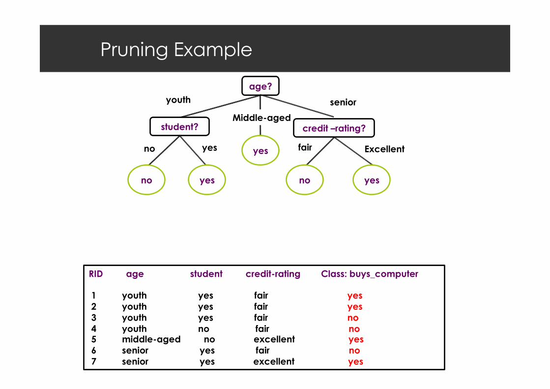
Pruning Example
age? youth
Middle-aged
senior
student?
yes no yes
no yes
RID age student credit-rating Class: buys_computer 1 youth yes fair yes 2 youth yes fair yes 3 youth yes fair no 4 youth no fair no 5 middle-aged no excellent yes 6 senior yes fair no 7 senior yes excellent yes
credit –rating?
fair Excellent
yes no
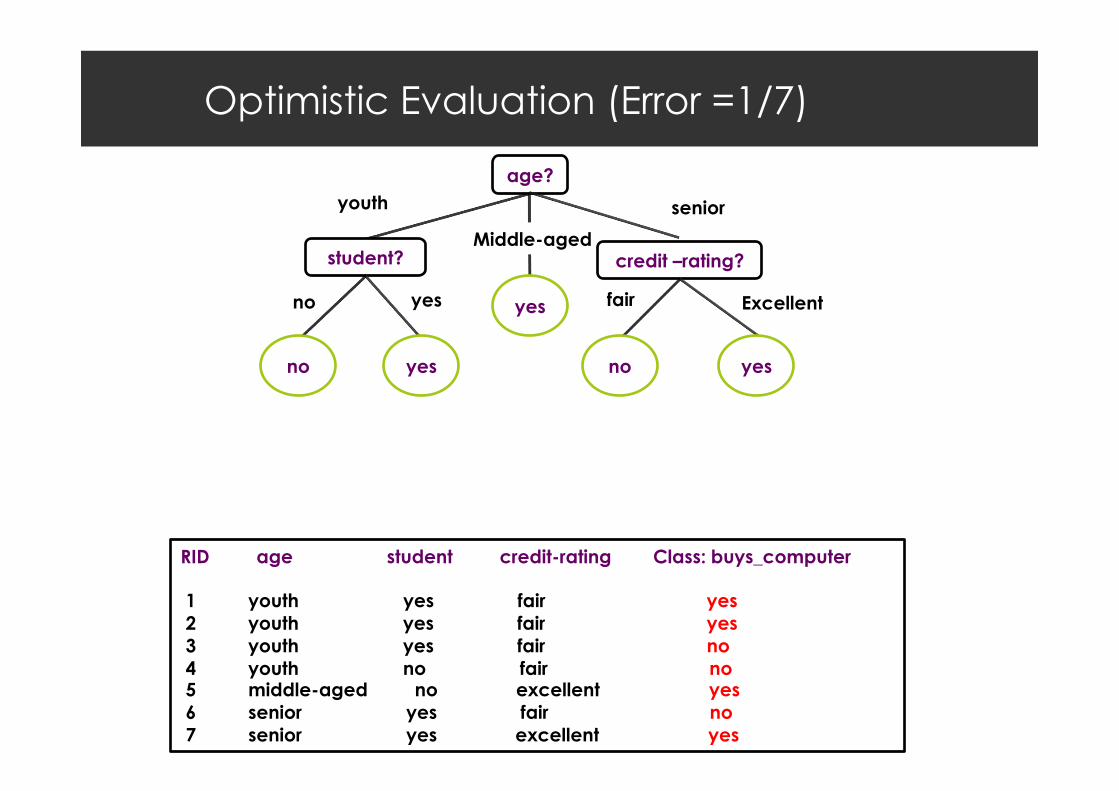
Optimistic Evaluation (Error =1/7)
age? youth
Middle-aged
senior
student?
yes no yes
no yes
RID age student credit-rating Class: buys_computer 1 youth yes fair yes 2 youth yes fair yes 3 youth yes fair no 4 youth no fair no 5 middle-aged no excellent yes 6 senior yes fair no 7 senior yes excellent yes
credit –rating?
fair Excellent
yes no

Evaluation using Validation Set (Error=3/7 )
age? youth
Middle-aged
senior
student?
yes no yes
no yes
RID age student credit-rating Class: buys_computer 1 youth no excellent yes 2 youth yes fair yes 3 youth yes fair no 4 youth no fair yes 5 youth no fair yes 6 middle-aged no excellent yes 7 senior yes excellent no
credit –rating?
fair Excellent
yes no

Pruning
age? youth
Middle-aged
senior
student?
yes no yes
no yes
credit –rating?
fair Excellent
yes no
RID age student credit-rating Class: buys_computer 1 youth no excellent yes 2 youth yes fair yes 3 youth yes fair no 4 youth no fair yes 5 youth no fair yes 6 middle-aged no excellent yes 7 senior yes excellent no

After Pruning (Error=1/7)
age? youth
Middle-aged
senior
yes
yes credit –rating?
fair Excellent
yes no
RID age student credit-rating Class: buys_computer 1 youth no excellent yes 2 youth yes fair yes 3 youth yes fair no 4 youth no fair yes 5 youth no fair yes 6 middle-aged no excellent yes 7 senior yes excellent no

Summary
¤ Decision Trees have relatively faster learning speed than other methods
¤ Conversable to simple and easy to understand classification rules
¤ Information Gain, Ratio Gain and Gini Index are the most common methods of attribute selection
¤ Tree pruning is necessary to remove unreliable branches

Question
Given dataset D and the number of attributes n, show that the computational cost of growing a binary decision tree is at most
n× |D |× log(|D |)


