Surface Rupture in KinematicRuptures Models for Hayward Fault
Scenario Earthquakes
Brad Aagaard
May 21, 2009
Surface Rupture from Kinematic Rupture Models
Holistic approach to calculating surface slip
• Objective
• Calculate surface slip from kinematic rupture models for largescenario earthquakes on the Hayward fault
• Use Monte Carlo technique to turn assemble probability densityfunction for surface slip from deterministic rupture models
• Constraints
• Spectral content of radiated seismic waves match observations• Reduce coseismic slip in regions with aseismic creep• Explicitly include constraints on surface slip (in progress)• Include estimates of afterslip (in progress)
1

Deterministic Kinematic Rupture Models
Complete description of spatial and temporal evolution of slip
• Spatial description of slip
• Background slip distribution (if imposing rupture dimensions)• Spatial variation of slip (slip heterogeneity)
• Temporal evolution of slip
• Hypocenter• Rupture speed• Slip time function
2

Rupture Lengths and Epicenters
We often impose a rupture length and epicenter in scenarios
Hayward South Hayward South + North
-123˚ -122.5˚ -122˚
37.5˚
38˚
0 50km
-123˚ -122.5˚ -122˚
37.5˚
38˚
0 50km
3
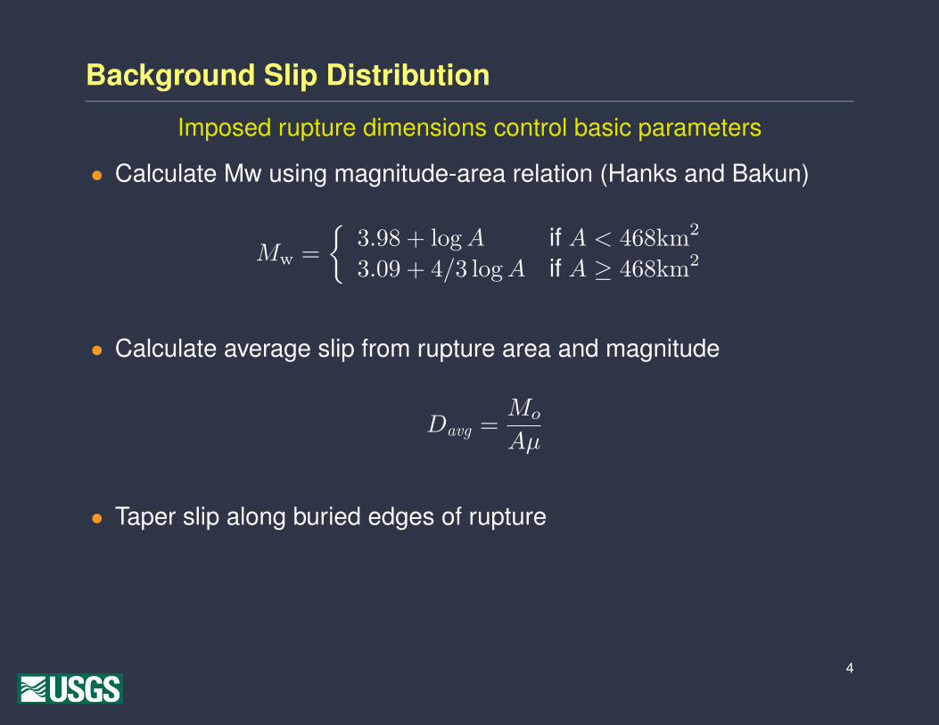
Background Slip Distribution
Imposed rupture dimensions control basic parameters
• Calculate Mw using magnitude-area relation (Hanks and Bakun)
Mw ={
3.98 + logA if A < 468km2
3.09 + 4/3 logA if A ≥ 468km2
• Calculate average slip from rupture area and magnitude
Davg =Mo
Aµ
• Taper slip along buried edges of rupture
4

Example of Background Slip Distribution
Hayward South + North, Mw 7.05
(NW) San Pablo Bay San Jose (SE)
5

Spatial Variation in Slip
Wavenumber spectra characterized by source inversions
• Somerville et al., 1999
P (kx, ky) =1
1 +(a2
xk2x + a2
yk2y
)2
log ax = −1.72 + 1/2Mw
log ay = −1.93 + 1/2Mw
• Mai and Beroza, 2002
P (kx, ky) =axay
(1 + a2xk
2x + a2
yk2y)H+1
, H ≈ 0.75
log ax = −2.5 + 1/2Mw
log ay = −1.5 + 1/3Mw
6
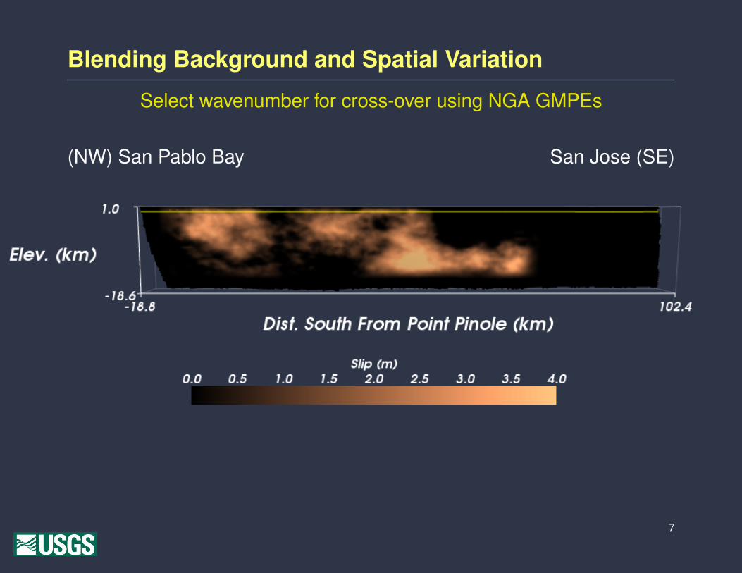
Blending Background and Spatial Variation
Select wavenumber for cross-over using NGA GMPEs
(NW) San Pablo Bay San Jose (SE)
7
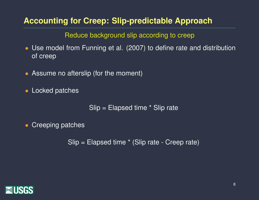
Accounting for Creep: Slip-predictable Approach
Reduce background slip according to creep
• Use model from Funning et al. (2007) to define rate and distributionof creep
• Assume no afterslip (for the moment)
• Locked patches
Slip = Elapsed time * Slip rate
• Creeping patches
Slip = Elapsed time * (Slip rate - Creep rate)
8

Creep on Hayward Fault: Funning et al. Model
Rate and distribution of creep constrained by geodetic data
9

Slip-predictable Approach: Background Slip
(NW) San Pablo Bay San Jose (SE)
10
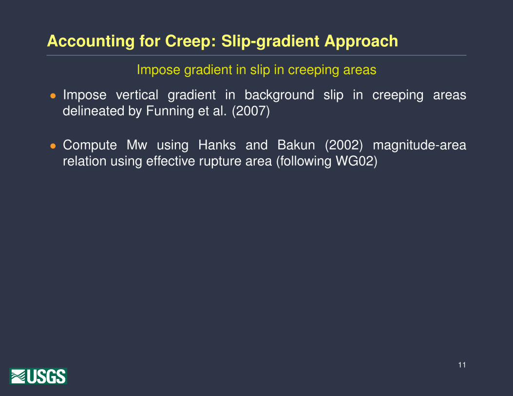
Accounting for Creep: Slip-gradient Approach
Impose gradient in slip in creeping areas
• Impose vertical gradient in background slip in creeping areasdelineated by Funning et al. (2007)
• Compute Mw using Hanks and Bakun (2002) magnitude-arearelation using effective rupture area (following WG02)
11

Accounting for Creep: Slip-gradient Approach
Impose gradient in slip in creeping areas
• Impose vertical gradient in background slip in creeping areasdelineated by Funning et al. (2007)
• Compute Mw using Hanks and Bakun (2002) magnitude-arearelation using effective rupture area (following WG02)
• Features
• Slip more likely to reach surface in larger events• More of the creeping areas rupture coseismically in larger events• Assume no afterslip (for the moment)
11

Slip-gradient Approach: Background Slip
(NW) San Pablo Bay San Jose (SE)
12

Hayward South + North Rupture Model
Slip distribution with 1 s rupture time contours
(NW) San Pablo Bay San Jose (SE)
13

Constraining Surface Slip
Wells and Coppersmith, 1994
• Maximum slip (strike-slip)
logDmax = −7.03 + 1.03Mw
• Average slip (strike-slip)
logDavg = −6.32 + 0.90Mw
• Empirical relation for coseismic slip without creep or afterslip
14

Surface Slip: Accounting for creep and afterslip
• Effect of creep on coseismic rupture
• Reduced magnitude for given rupture area (WG02 effective area)• Use reduced magnitude in slip/magnitude relation
• Incorporating afterslip (some assumptions)
• Afterslip releases stress concentrations following rupture• Near-surface slip driven by greater slip at depth
15

Coseismic Slip from Scenario Rupture Models
Fine-tune stochastic parameters and blending for better match
W&C, 1994 Max. Slip. (m) Avg. Slip (m)
Mw 6.76 0.86 0.58
Mw 7.05 1.7 1.1
Hayward South, Mw 6.76
-20 -10 0 10 20 30 40 50 60 70Distance south along strike from Pt Pinole (km)
0
1
2
Slip
Mag. (m
)
Hayward - Calaveras
Hayward South + North, Mw 7.05
-20 -10 0 10 20 30 40 50 60 70Distance south along strike from Pt Pinole (km)
0
1
2
Slip
Mag. (m
)
Hayward - Calaveras
16
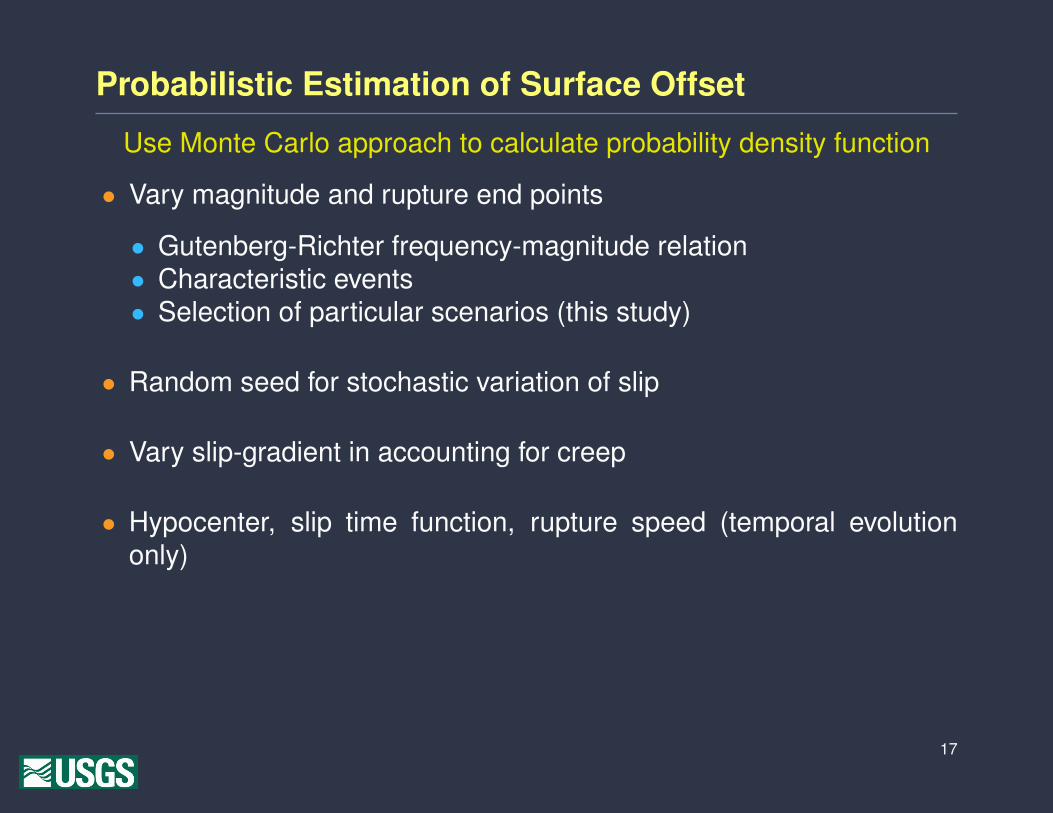
Probabilistic Estimation of Surface Offset
Use Monte Carlo approach to calculate probability density function
• Vary magnitude and rupture end points
• Gutenberg-Richter frequency-magnitude relation• Characteristic events• Selection of particular scenarios (this study)
• Random seed for stochastic variation of slip
• Vary slip-gradient in accounting for creep
• Hypocenter, slip time function, rupture speed (temporal evolutiononly)
17

Long-Term Research Issues
Incorporate more physics into rupture modelsSpontaneous dynamic rupture models include fault constitutive behavior(but are currently poorly constrained)
• Do fault constitutive model parameters vary in the near surface?
• Stable sliding at shallow depths instead of unstable sliding• Variation in friction (cohesion and overburden pressure)
• Does coseismic slip decrease at shallow depths?
• Does surface slip have the same spatial variation as deep slip?
• Is surface coseismic slip slower/faster than slip at depth?
• How does creep affect slip?
• Does effect of creep vary with earthquake magnitude?• Correlation of afterslip with creep?
18


