1
Survey protocol for fisher denning season: methods for informing
denning protection measures
Jody Tucker1, Rebecca Green2, Kathryn Purcell2, and David Green3
1 U.S. Forest Service, Pacific Southwest Region 5 2 U.S. Forest Service, Pacific Southwest Research Station 3 Institute for Natural Resources, Oregon State University
Protocol Overview
The intent of this protocol is to provide a means to assess whether fisher (Pekania
pennanti) occupy an area during the denning (i.e., reproductive) period. In areas within a pre-
existing Limited Operation Period (LOP) designation, this protocol can be used to determine
with high confidence whether or not a project area is occupied by fisher during the denning
season and, if found unoccupied, could potentially shorten the LOP. Conversely, in areas
without a current LOP but with potentially suitable fisher denning habitat, this survey protocol
can inform at a broad scale whether an LOP may need to be implemented. Unlike some other
wildlife protocols, the methods described here cannot be used to identify a specific den site that
can then be protected; the cryptic behavior of denning female fishers using tree cavities to care
for kits makes identifying the location of an active den nearly impossible without use of radio
telemetry. Instead, this protocol is designed to detect a highly mobile carnivore within a home
range that supports fisher resource needs during reproduction. Consequently, the methods are
geared towards confirming with high confidence that a denning female is not present in a project
area. In cases where a this protocol is used to detect fisher during breeding season to implement
an LOP in a project area, an effective buffer would need to be quite large (comparable to a
female home range in size).
The behavioral characteristics of fishers during the reproductive period reduces the
likelihood of detecting them quickly even when present. As a result, the survey period described
in this protocol is a minimum of 35 days (and will thus take sufficient planning to get an early
start) and the LOP may only be shortened (i.e., not completely waived). For managers that wish
to shorten an LOP, this protocol will be most useful in areas with low suitability for fisher and
with a high benefit associated with early access to conduct management activities. Conversely,
for managers that wish to better protect denning females in areas where data are lacking, this
protocol provides a tool to assess with a high degree of certainty whether or not fisher are present
during the denning season, and may reflect reproduction.
Surveying during the denning season introduces unknown risks by potentially altering
fisher behavior or by attracting other carnivores, including potential predators (e.g., bobcat,
mountain lion), to the bait and lure used in the surveys. Therefore, surveys to document fisher
occurrence that are not related to LOP considerations should be conducted outside of the
reproductive season. Also, to minimize potential negative consequences of bait and lure in a
2
denning area, we recommend discontinuing use of these attractants at cameras once a fisher is
detected until denning season has concluded.
Fisher reproductive ecology background
Fishers are elusive carnivores that are difficult to observe throughout the year, but they
are arguably even more secretive during the reproductive period. Females initially give birth
(i.e., parturition) and care for their young kits (usually 1-3) at a natal den (a live tree or snag with
a cavity). In the southern Sierra Nevada, female fishers typically give birth between mid-March
and the second week of April (Green et al. 2018). Although there is some variation in timing of
parturition across the range of fisher in North America, data indicate a relatively limited and
consistent window between early March and mid-April (Green et al. 2018). Mating occurs
within 1-2 weeks after birth; during this time males actively seek out females at natal dens and
other locations. After a few weeks or more in a natal den, females typically move their kits to a
series of maternal dens (e.g., live trees, snags, occasionally logs with cavities). Female fishers
on the Sierra National Forest used an average of 3.5 structures in a reproductive season (Green et
al. 2018). Female fishers leave little to no visible sign of their presence at den sites, tend to
remain quiet and hidden when in or near the den, and come and go infrequently to forage; as a
result, there is no easy way to identify a particular tree as an active den or follow a fisher to a den
(as might occur when locating an owl nest) unless individuals are fit with radio transmitters.
Protocol development
To specifically assess female detectability during the denning season, we implemented a field
study using systematic camera surveys across the Pacific Southwest Research Station’s (PSW)
Kings River Fisher Project (KRFP) in the Sierra National Forest where an on-going fisher study
was using GPS radio collars to track individual fishers and locate dens. We analyzed fisher
detections from these camera surveys in combination with spatial data from individual radio-
collared fishers (i.e., den locations, GPS points) to evaluate whether female fishers could be
reliably detected using remote cameras during the reproductive period. This study provided the
data to determine 1) detection probabilities for denning females, 2) detection distance to inform
camera spacing, and 3) length of time needed for an effective survey. A brief description of this
study is provided below. Additional details are included in Appendix A.
Summary: Female fisher LOP detectability study
PSW personnel captured and attached GPS collars to 34 fishers (20 females and 14
males) in the KRFP study area between Oct 2017 - Feb 2018 (see Green et al. 2018 for trapping
and handling protocol). By early March 2018, there were working GPS collars on 8 females
known or estimated to be of reproductive age (≥ 2 years); 7 of these females initiated natal dens,
6 appeared to den successfully, and 1 did not den. Between March and June of 2018 we located
fisher reproductive dens using the VHF signal from the GPS collars combined with ground
3
telemetry; during spring of 2018, the 6 successful reproductive females used an average of 4.2
den structures (range of 3 to 5).
Although we did not know in advance where collared females might den, all collared
adult females were known individuals with known home range and den site data from prior
years. This information was used to inform the camera survey area so cameras could be
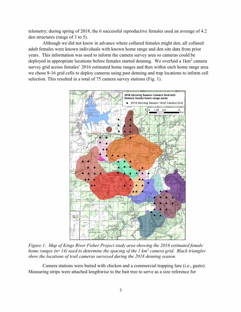
deployed in appropriate locations before females started denning. We overlaid a 1km2 camera
survey grid across females’ 2016 estimated home ranges and then within each home range area
we chose 8-16 grid cells to deploy cameras using past denning and trap locations to inform cell
selection. This resulted in a total of 75 camera survey stations (Fig. 1).
Figure 1. Map of Kings River Fisher Project study area showing the 2016 estimated female
home ranges (n=14) used to determine the spacing of the 1 km2 camera grid. Black triangles
show the locations of trail cameras surveyed during the 2018 denning season.
Camera stations were baited with chicken and a commercial trapping lure (i.e., gusto).
Measuring strips were attached lengthwise to the bait tree to serve as a size reference for
4
morphological measurements and sex identification. Hair snares were deployed to collect
genetic samples for both individual and sex identification of visiting fishers.
For each camera station that detected a fisher via photograph(s), we attempted to assign
both sex and individual identifications using three successive methods 1) genetics from hair
samples, 2) morphological measurements from the measuring strip, and 3) expert opinion
informed by physiological characteristics and GPS collar location information. We used
detection/non detection data for each of the 7 denning females at the camera array to model the
probability of detecting each individual female fisher on trail cameras as a function of 1) the
distance between their den centroid and each trail camera, 2) the number of days the camera was
operating, and 3) the camera type (i.e., whether the camera was a Bushnell Aggressor).
We found female detectability was significantly affected by both survey length and
camera model, with the minimum survey length required to reliably detect a female fisher to be >
35 days. Camera model results also indicated that the choice of camera model is critical in
effectively detecting females; consequently, camera models used in protocol surveys must meet
certain defined minimum specifications. We used detection probability estimates as a function
of camera distance to determine the required grid spacing to achieve a high detection probability
for fisher (>0.95 mean detection probability). Grid spacing varied with the number of cameras
that are deployed. Based on our findings, a 700 m camera spacing and >3 cameras is required
for small project areas (<250 acres) whereas >4 cameras and a 1000 m spacing is sufficient for
large project areas (>250 acres). A detailed description of the full study methods and results are
described in Appendix A.
Fisher denning season survey protocol
This protocol can be used to:
a) potentially shorten the LOP in an area with a pre-designated fisher denning LOP (i.e.,
predicted suitable fisher denning habitat in the Southern Sierra Nevada (SSN), but where
it is unknown if females are currently denning) or
b) designate an LOP* in an area where fisher denning status is unknown and no current
management restrictions exist, but which has potential to contain dens based on habitat
characteristics and/or geographic location relative to known or predicted occurrence.
If a fisher is detected during a spring survey (female or male), we advise that survey
efforts conclude immediately after detection to minimize any possible impacts to reproductive
females in the area. Other fisher surveys not associated with informing an LOP are best
implemented outside of the denning season (i.e., July to September) to minimize potential
impacts of surveys during the denning season (e.g., bait or lure altering fisher behavior or
attracting predators to occupied areas).
Protecting reproductive females is one of the most critical factors for species
conservation, so we have designed this protocol to detect fishers during denning season with a
high degree of certainty (>95% detection probability). It is crucial to follow these instructions

5
carefully to ensure fishers are detected effectively as even seemingly minor changes to the
protocol (i.e. battery type, camera model) can have a significant impact on detection rates.
* This protocol is designed to detect a fisher home range during the denning season. This is not
a detection protocol that identifies a specific den location. Consequently, any LOP area
designated as a result of a detection from this protocol should approximate the size of a female
fisher home range in the local survey area.
Establishing the area to be surveyed
1) Identifying the project area:
The project area is defined as all lands delineated for the proposed project that
may be subject to activities potentially impacting fisher denning habitat (e.g.,
modification, direct injury, repetitive or extended noise disturbance, or any other
means). Management activities subject to LOP restrictions are listed in Table 7 of the
SSN Fisher Conservation Strategy (Spencer et al. 2016). The project area is(are) the
polygon(s) that forms the footprint of the proposed project.
2) Delineating the survey area:
The survey area is defined as the project area buffered by an additional 200 m
from the outside perimeter of the project area. The 200 m buffer ensures denning
locations adjacent to or just outside project boundaries that may be impacted by project
level disturbances are included in the survey area. This distance corresponds to
approximately half of the mean distance females moved between dens during the
denning season (Green 2017).
Camera spacing
Camera spacing requirements for small project areas (i.e., small number of cameras) and
large project areas (i.e., larger number of cameras) are different because detectability improves
as the number of cameras deployed in an area increases. Larger survey areas can space cameras
farther apart due to the overall greater number of cameras compared to a smaller survey area.
1) For small project areas <250 acres, cameras should be spaced a maximum of ~700 m
apart (+/- 50 m to allow for finding the best available habitat/site characteristics for
camera installation). A minimum of 3 cameras is required for 700 m spacing.
2) For large project areas >250m acres that inherently will use a greater number of
cameras – spacing between cameras can be increased to a maximum of 1000 m (+/- 100
m) with a minimum of 5 cameras in the survey area.
While data indicated that small and large project areas could potentially be
surveyed with only 2 and 4 cameras respectively, this protocol requires an
6
additional camera to compensate for likely non-functional days and thus help
ensure achieving a valid survey effort within a 35-day period. Cameras often
malfunction or become inoperable for a variety of reasons (e.g., bears and
other wildlife can alter the camera view or render cameras inoperable in other
ways, heavy rain or snow may block or fog camera view). Cameras may also
be less effective if checks and rebaiting are not regularly completed.
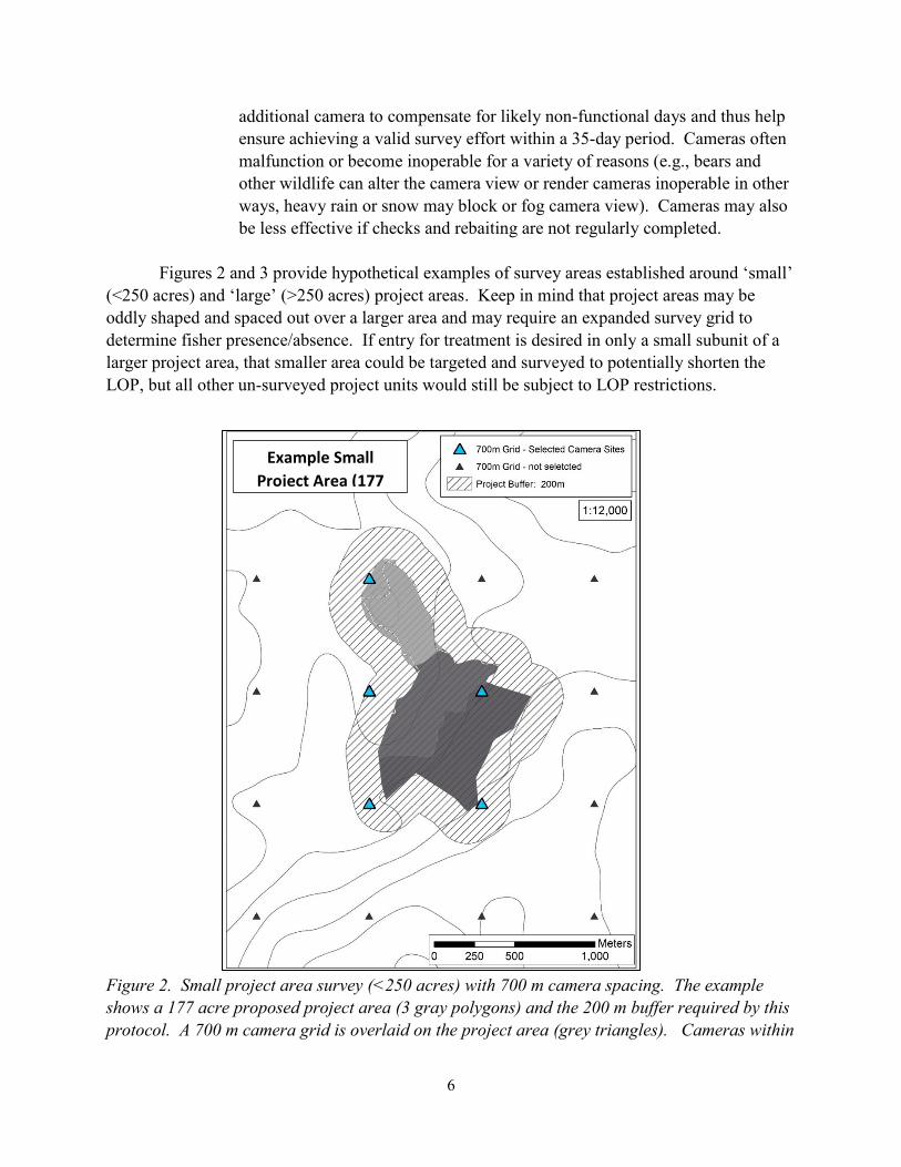
Figures 2 and 3 provide hypothetical examples of survey areas established around ‘small’
(<250 acres) and ‘large’ (>250 acres) project areas. Keep in mind that project areas may be
oddly shaped and spaced out over a larger area and may require an expanded survey grid to
determine fisher presence/absence. If entry for treatment is desired in only a small subunit of a
larger project area, that smaller area could be targeted and surveyed to potentially shorten the
LOP, but all other un-surveyed project units would still be subject to LOP restrictions.
Figure 2. Small project area survey (<250 acres) with 700 m camera spacing. The example
shows a 177 acre proposed project area (3 gray polygons) and the 200 m buffer required by this
protocol. A 700 m camera grid is overlaid on the project area (grey triangles). Cameras within
Example Small
Project Area (177
acres)
7
200 m of the project perimeter are selected for the fisher denning surveys (larger blue triangles).
In this example, 5 cameras would be required to survey this project area.
Habitat and camera station placement
Cameras should be placed in areas where habitat elements or features commonly
associated with fisher are present to the extent possible because detectability of fishers can be
significantly influenced by habitat characteristics at the survey site (Tucker, Green and
Matthews, pers. com.). Cameras can be moved within a specified range from the prescribed grid
spacing to find the best available habitat in which to install the cameras (up to +/- 50 m for the
smaller 700 m grid or +/- 100 m for the larger 1000 m grid).
Preferred habitat characteristics of female fisher home ranges in the southern Sierra
Nevada include: moderate to high canopy cover (≥60%), high basal area, presence of mature or
large diameter trees, contiguous patches of dense and mature forests, moderate to steep slopes,
mixed conifer-hardwood forests containing mature California black oaks, and proximity to
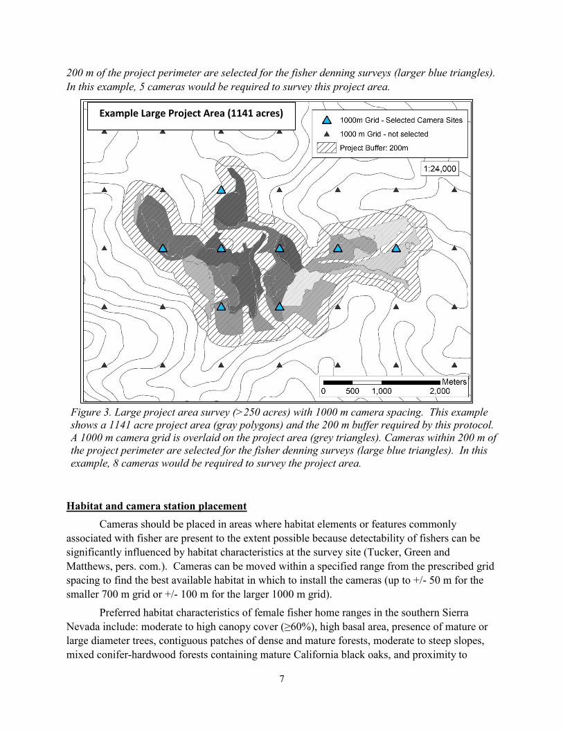
Figure 3. Large project area survey (>250 acres) with 1000 m camera spacing. This example
shows a 1141 acre project area (gray polygons) and the 200 m buffer required by this protocol.
A 1000 m camera grid is overlaid on the project area (grey triangles). Cameras within 200 m of
the project perimeter are selected for the fisher denning surveys (large blue triangles). In this
example, 8 cameras would be required to survey the project area.
Example Large Project Area (1141 acres)
8
permanent streams (Zielinski et al. 2004, Popescu et al. 2014, Spencer et al 2015, Green 2017).
At the scale of the individual structure (e.g., tree, log) or microsite (e.g., cavity, platform),
denning and resting fishers in the southern Sierra Nevada often use large diameter hardwoods
with cavities and large limbs as well as large diameter conifers (i.e., live trees and snags) with
cavities, platforms, or other signs of decay (see Green et al. 2019 for a range of dbh
measurements and example photos). For additional details on fisher habitat characteristics in the
SSN refer to section 4 of the southern Sierra fisher Conservation Assessment (Spencer et al.
2015). If implementing this protocol outside of the SSN, alternate habitat characteristics may be
relevant to local conditions. A summary of fisher habitat characteristics across western states is
detailed in Chapter 7 of the western states fisher Conservation Assessment (Lofroth et al. 2010).
Survey Period
1) Based on the timing of fisher reproduction, the earliest start date for these surveys is
March 15
2) Minimum length of survey: 35 functional days.
3) Functional days must account for inoperable days due to camera malfunction. *If a
camera becomes inoperable during the survey those days do not count toward minimum
survey length. Inoperable cameras days may include, but are not limited to:
a) Bears or other wildlife knocked the camera such that the bait is no longer in the
photo frame or caused other malfunction (e.g., opened camera)
b) Camera stopped functioning between visits (i.e., the bait is gone but no photos of
animals are on the camera)
c) SD card error such that images are not recorded, card is corrupted, or card is lost
with no backup
d) A technician forgot to turn on a camera after servicing
4) Cameras should be checked, rebaited, and lure reapplied every ~7 days (details on checks
provided in a subsequent section) such that there is a minimum of 5 checks for each
camera (6 visits total including the initial set-up).
Fisher detections
Trail camera photos should be reviewed for species detections in an office setting on a
laptop or desktop computer. Viewing photos in the field on the trail camera or photo viewer can
be helpful to ensure that the camera is working properly and that the field of view is appropriate,
but these options are generally inadequate to evaluate detection of species. Animals are often
difficult to spot, partially obscured, or only present briefly or at night in dark conditions in the
photo. As a result, fishers can be easily missed during field review due to a combination of small
screen sizes and difficult lighting – so additional review on a larger screen in an office setting is
essential.
9
For the purposes of this protocol, we consider any photo of a fisher to be a valid positive
detection, regardless of whether it is a male or female due to the difficulty in accurately
determining sex via photos alone. Genetic identification is not likely to be logistically feasible in
most situations as it can be expensive, time consuming, and involves a waiting period to obtain
results. Sex identification using photo measurements and expert identification are not readily
available and not infallible. Further, during the reproductive season, males visit females at natal
den sites for mating opportunities; male presence is suggestive of a denning female during this
time of year. Several examples from our field study displayed in figures in Appendix A support
this idea, with males regularly being detected at cameras in the vicinity of reproductive females
and their dens. Once a fisher is detected we recommend discontinuing the surveys. This reduces
survey effort and cost and helps avoid any potential negative impacts such as drawing in
predators to baited and lured cameras in areas where females may be denning.
Camera model selection
Different models of trail cameras vary widely in their ability to detect target species
depending on specifications such as trigger speed, recovery time (i.e., minimum time needed
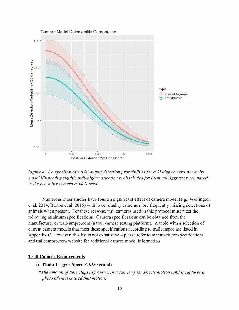
between triggers), and detection distance. We found a statistically significant difference in
detectability between different camera models, with the newest camera model used in the
surveys (2017 Bushnell Aggressor No Glow 20 MP) having considerably higher detectability
compared to other models (Figure 4).
10
Figure 4. Comparison of model output detection probabilities for a 35-day camera survey by
model illustrating significantly higher detection probabilities for Bushnell Aggressor compared
to the two other camera models used.
Numerous other studies have found a significant effect of camera model (e.g., Wellington
et al. 2014, Burton et al. 2015) with lower quality cameras more frequently missing detections of
animals when present. For these reasons, trail cameras used in this protocol must meet the
following minimum specifications. Camera specifications can be obtained from the
manufacturer or trailcampro.com (a trail camera testing platform). A table with a selection of
current camera models that meet these specifications according to trailcampro are listed in
Appendix C. However, this list is not exhaustive – please refer to manufacturer specifications
and trailcampro.com website for additional camera model information.
Trail Camera Requirements
a) Photo Trigger Speed <0.33 seconds
*The amount of time elapsed from when a camera first detects motion until it captures a
photo of what caused that motion.

11
b) Photo Recovery: < 2.0 seconds
* The amount of time required for a camera to rearm itself and take a second triggered
photo after the first triggered photo is captured.
c) Infrared Flash – no glow or low glow cameras
* minimize ‘spooking’ an animal with a white flash during a night detection
Camera Station Instructions:
1) Before installing cameras in the field, practice with your cameras to make sure you are
familiar with their operation and how to change the settings.
2) We will not go into extensive detail on aspects of basic field work that we expect people
conducting these surveys will have (e.g., safety in field navigation, use of maps).
However, we emphasize that these types of surveys usually require that field assistants
are capable of hiking long distances over rough terrain and navigating confidently with a
handheld GPS unit. Fishers frequently occur in areas with extensive cover and steep
slopes that can be difficult to navigate, thus field personnel need to be prepared and
trained accordingly.
Site Selection
1. Camera and bait trees should be between 3.0-4.0 meters apart. Correct spacing is more
important than the camera aspect.
2. Locate two trees that are the proper distance apart and allow the camera to face
approximately North (camera aspect between ~320 and 40 degrees) to reduce the
likelihood of sun-caused false triggers.
3. Bait tree should be a minimum of ~20 cm DBH, although a larger tree is preferable (trees
smaller than 20 cm DBH can be used if the only option).
4. Whenever possible for safety considerations, DO NOT USE SNAGS as camera or bait
trees.
5. Trees should be well shaded, with adequate canopy cover and placed in the best possible
fisher habitat available in the area.
6. Avoid trees with small lower branches or nearby saplings or shrubs with flexible
branches as wind in these smaller branches can cause numerous false triggers of the
camera. Clear away any small dead branches that would obstruct view of the camera, or
that would set off the camera sensor with wind or temperature changes.
Bait Installation
The bait type for this survey will be raw chicken leg quarters which are enclosed in
socks, and attached to the tree. Using a sock has several benefits, but the main purpose here is to
make it harder for an animal to get the bait quickly – thus increasing the chance of triggering the
camera and obtaining photos. Bait should be installed first in order to properly aim camera.
12
1. Attach bait to tree at approximately chest height
2. To attach the bait:
a. Place a chicken leg quarter (or multiple smaller pieces totaling an equivalent size)
inside of a long sock and tie the open end closed with a knot. Attach bait sock to
the tree with a minimum of 2 fencing staples (preferred) or aluminum nails on
each side and the top and bottom of the bait sock (see example photos). OR
b. In areas where putting staples or aluminum nails in trees is undesirable, an
alternative lower impact approach is to tie a long piece of twine securely around a
tree at chest height, then individually tie 2 bait socks to the circle of twine so that
they hang along the bole of the tree. As wildlife may have an easier time
obtaining this bait compared to bait that is nailed to the tree, using 2 socks hung
separately can help ensure that photos are obtained (see examples). For this
option using one chicken leg in each sock (not whole quarters) is sufficient.
3. Nail a sign with a clearly readable site ID approximately 4-6 inches above the bait.
4. Apply Gusto scent lure (~2 tsp.) to the tree with a stick just above the bait height (and
within the camera frame)
5. Shove the lure application stick into ground at the front base of bait tree, directly below
the bait and within the camera frame. Animals often investigate or rub on the lure stick
so it is important to include it in the photographed area.
Camera Installation
To reduce chance of theft or bear damage, we recommend placing the camera in a lockable
security box or securing it to the tree with a locking cable.
Camera accessories and settings:
1. Lithium batteries are required. Trigger speed is slowed by alkaline batteries in cold
temperatures and lithium batteries will last much longer.
2. Minimum SD card size 2GB to ensure sufficient room for photos
3. Camera settings
a) Photos per trigger/ Burst setting / Number of photos = 2
b) Interval / quiet period (i.e., min time elapsed between next trigger) = 5 seconds
c) Image size: Recommend 3-8 MP. Smaller image sizes may lack resolution and larger
image sizes take up excessive space on memory card.
d) Date time stamp set in 24 hr military time (ensure that date/time is set correctly)
e) Sensor level = high
Installing the camera:
4. Attach camera to the tree at approximately chest height using a locking cable, lashing strap, or
ratchet strap
13
5. Adjust the camera so the photo frame includes the entire base of the bait tree to the top of the
site ID sign. Take a test photo by standing at the bait tree and waving hand back and forth in
front of the bait for ~15 seconds.
6. Check the test photo using either the camera screen or an external photo viewer or digital
camera to make sure that camera is properly aligned as follows:
a) the bait tree should be centered left/right in the photo.
b) the photo includes the SITE ID LABEL, LURE, BAIT, and BASE OF TREE
c) Many animals investigate the bait from the bottom up (i.e., climbing up from below,
walking around base of tree) and therefore, it is very important to include the base of tree
in the photo frame.
d) If the camera is moved after test photo, take another test photo as even small
movements of the camera can significantly impact the photo frame.
e) If needed, adjust the camera positioning:
Adjust camera laterally by sliding the camera left or right on the strap
Adjust camera up/down with a door stop or by placing a stick or small
piece of bark behind the top of the case to adjust the angle of the view
If more up/down movement is needed, try moving the entire camera setup
up or down on the tree
Note that it is better to have the camera either level with the ground or up
high enough to angle down slightly. Avoid angling the camera up, as the
view is likely to be obscured if there is precipitation during the survey.
7. Once the camera is positioned correctly, double-check camera settings, time stamp and
battery level
a) If battery level is below 80%, replace batteries (lithium batteries are known to go from
reading high % charge to low charge very rapidly so, need to change if <80%)
b) Make sure to recheck settings. Often when batteries are replaced, or if the camera is
unused for a while, the camera settings reset or change.
c) Wipe camera and case with a wildlife scent ellimination wipe (available through many
hunting or sporting goods retailers) before locking and turning on.
d) Turn camera to ON position or ARM camera (depending on model), place camera in
security case, and lock case.
e) Flag camera tree with double flag behind camera within 10 m to facilitate relocating
camera for future checks (do not hang flagging behind the bait tree as this can cause false
camera triggers).
f) Fill out camera installation section of data form noting camera settings and record GPS
coordinates in either UTM or Lat/Long.
14
Checking the camera (weekly service visits)
1. Photo and Video Collection
a. Unlock and open security case and turn off camera.
b. View and inspect photos/videos to determine if a fisher is present. If a fisher is
definitively present, the survey can be discontinued. However, photos can be difficult to
review in the field on the trail camera’s viewer, so if there is any uncertainty in species
detections leave cameras installed until photos can be thoroughly reviewed at the office
or on a larger laptop screen.
c. Pull field SD card each visit and replace with a new card. This SD card is the only
copy of the data. Carefully transport the used field SD card back to the office for
immediate download & backup. Note you will likely want to label SD cards with unique
identifying numbers in advance and provide secure transport cases for blank cards and
cards with data (i.e., pelican case or prescription-type vials with locking caps).
d. Replace bait if missing or in bad condition. If bait seems undisturbed and in good
condition can leave for one additional visit. Maximum bait time in field = 2 weeks.
e. All old bait should be removed from the field. Do not discard bait in the field near
camera as it might impact attraction to new bait at the camera.
2. Complete weekly visit section of data form
3. Gusto scent lure: Reapply at each visit – 1 tsp. in same location as previous visit
4. Verify Camera Settings:
a. Double-check all camera settings. **Date and time settings often randomly reset
within a check period to essential to double check date and time is still accurate
b. Replace batteries if <80%
c. If it appears that the camera is malfunctioning, replace with spare camera and write
detailed comments on data forms about how its malfunctioning
d. Take a test photo
e. Check the test photo; adjust the camera if needed
f. Turn camera on (or arm camera), lock, and walk away through camera frame to record
a start photo for that survey period
15
General Equipment Needed for Camera Station setup:
Camera Setup Equipment:
Camera - recommend labeling individually with unique identifier in advance
Security/bear case (optional, but recommended)
Camera strap
Lock (optional, but recommended)
Compass
Meter/dbh tape (for measuring camera spacing)
Door stop (optional, useful for positioning camera)
Dry bag/stuff sack (for keeping camera away from bait)
Photo viewer or digital camera (if no viewer screen on camera)
Batteries (lithium) for camera - enough for camera and full set of spares
Memory card for camera (SD, 2 or 4 GB) - recommend labeling individually in advance
GPS unit (with spare batteries)
Data form (Appendix D)
Flagging
Scent Killer Wipes or Spray
Bait Tree Setup Equipment:
Fencing/U staples and/or nails OR
Roll of strong twine (if trying to avoid staples or nails in trees)
Aluminum nails or other form of attachment for placard
Placard (station sign – recommend write in the rain or other weather resistant surface)
Bait sock (recommend long sock of relatively thin material – like a men’s dress sock)
Chicken (legs work best with socks)
Gusto scent lure
Hammer/fencing tool
Multi-tool or small scissors for cutting twine
Fine point sharpie

16
Checking and surveying the cameras
General Camera Check Equipment
Blank memory cards – SD (in some sort of protective case)
Protective case to transport SD cards with data
Hammer/fencing tool
Multi-tool or small scissors
Photo viewer or digital camera to review photos
Extra batteries (lithium for camera)
Gusto
Extra placard
Extra camera
New bait sock (chicken can be put in socks in advance, left in freezer, transport in cooler)
Staples , nails, and/or twine
Fine-point sharpie
Data form (Appendix D)
17
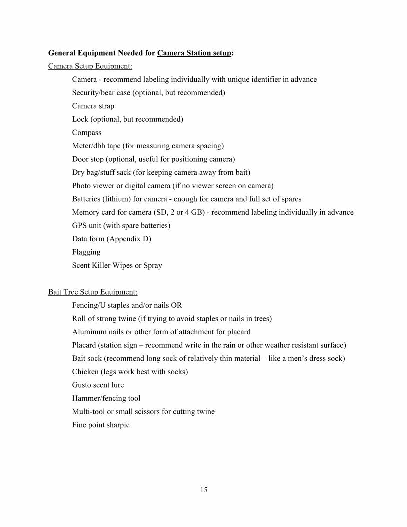
Example Photos: Camera stations
Photo A below shows a camera in a locked metal box attached to a tree with a ratchet strap at a
little above chest height. Photo B shows the twine-chicken sock bait method. In this case, twine
is tied tightly around the tree at dbh height. Then 2 socks, each containing a chicken leg, are tied
individually to the twine and left hanging. Photo C shows a sock containing a chicken quarter
tied with a knot then nailed to the tree. Photo D shows the entire set up (camera on left, bait on
right). Recommended distance between camera and bait is 3-4 m; the trees in this example
reflect the furthest appropriate distance (~4 m). Photo E shows an actual photo from our
surveys, including the placard, measuring strip, and a female fisher. Note that we used mesh
wire in photo E (not the currently recommended sock method).
A B C
D E
18
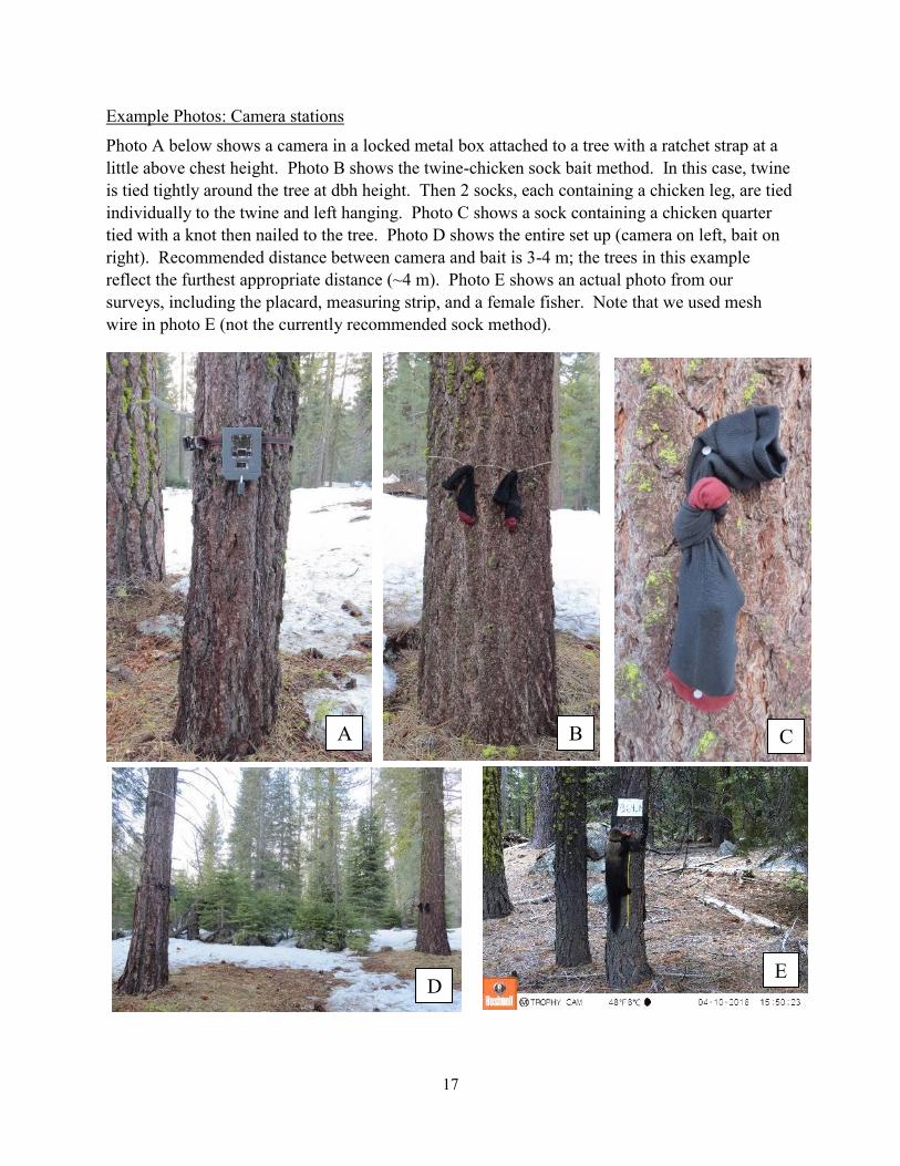
Example Photos: Female fishers
These photos may help in identification of
fishers at camera sites. Photo A shows a
juvenile female fisher at a capture. Note
the lighter fur on her head and shoulders
relative to the darker fur on her legs,
haunches, and tail. The “blondness” of the
head and shoulders varies by individual and
season, but the legs, haunches, and tail of
fishers in the SSN is almost invariably very
dark brown. The remaining photos (B-E)
were all taken by remote cameras of females at dens (not baited) and reflect some of the
differences in appearance of fishers in different lighting as well as they look going up and down
trees.
A
E D
C B
19
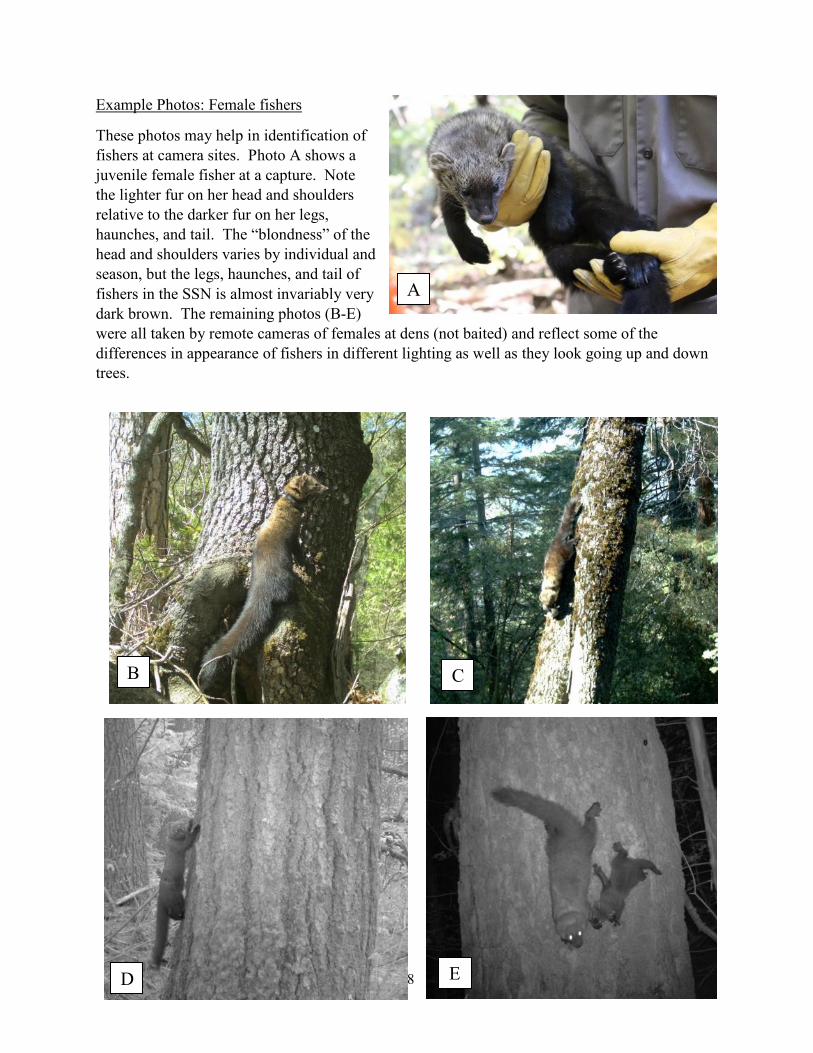
Example Photos: Male and Female Fishers at bait stations
These photos show examples of male and female fishers detected at baited camera stations
during our surveys. Note we used a different method (chicken wire) and hair snares at these
stations (we are not recommending these approaches, just wanted to include the sample photos).
The upper photos A and B are female fishers at bait stations (daytime and nighttime). The lower
photos C and D are male fishers at bait stations (daytime and nighttime).
A
B
A
C
D
20
Appendix A
Detailed Methods/Results: Female Denning Season Detectability Study (March –June 2018)
GPS collar attachment and location of reproductive dens
As part of an on-going study of fisher ecology conducted by Pacific Southwest (PSW)
Research Station, field personnel followed established protocols to trap fishers and fit them with
GPS collars between October 2017 and February 2018 on the Kings River study area (See Green
et al. 2018 for details on trapping and handling methods). Female and small male fishers were
fitted with Lotek LiteTrack 40 GPS collars (45 grams) while medium to large male fishers were
fitted with Lotek LiteTrack 60 GPS collars (63 grams). Both collar models had remote download
capability (RF) and used the SwiftFix option. In addition, handmade breakaway devices were
added to each collar to reduce chance of injury if fishers were not recaptured. During the 2017-
2018 trapping period, PSW personnel captured 34 fishers (20 females and 14 males). Four adult
females either dropped or experienced collar failure just prior to or at the beginning of the den
season. By early March 2018, we had working GPS collars on 8 females known or estimated to
be of reproductive age, and thus potentially available for inclusion in the camera survey effort.
Of these 8 females, 6 appeared to den successfully, 1 initiated a den that subsequently appeared
to fail, and 1 did not appear to give birth. Our camera surveys covered territories of all 8 adult
females.
We used the VHF signal on the GPS collars to locate the reproductive dens of female
fishers between March and June 2018. The basic technique to locate dens is for field technicians
to hike to the locations of adult females that appeared to be inactive (especially in the morning
hours) and locate the structure where they were resting. If a female was found to be in a tree
with a cavity on more than one occasion over a few days, the tree was identified as a
reproductive den. See Green et al. (2017) for additional details on the techniques used to identify
and monitor dens. Females that both denned successfully and retained working GPS collars for
the 2018 denning season used an average of 4.2 den structures (range of 3 to 5). One female
dropped her collar in her second den tree, but we were able to continue to monitor her activity
through use of remote cameras because she continued to use the same tree for much of the den
season.
Camera Survey
We overlaid a 1km2 camera survey grid across the area of GPS collar deployment using
the fishnet tool in ArcGIS 10.5.1 (ESRI 2017). We then used denning and capture locations
from 2016 to select a subset of grid cells that overlapped with past denning female home ranges
and den sites. We selected 8-16 camera grid cells dependent on the size of the home range from
each of 7 female denning areas, each of which overlapped with the home ranges of 1-2 known
females resulting in a total of 75 survey grid cells.
Trail cameras were deployed systematically throughout Kings River in the spring of
2018. As the project areas are quite variable in terms of size and configuration on the landscape,
and we wanted our detectability results to pertain to a wide range of habitats, camera locations
21
were not selected based on habitat suitability at the camera site. Difficult site access made it
unfeasible to place the camera at 1 km spacing for a minority of grid cells; closer spacing was
necessary at a subset of grid cells but all cameras were >500m from the nearest camera. We
installed cameras in two batches because we hypothesized that female detectability may increase
during the denning season as kits become older and more mobile: early denning season
deployments (3/13-4/3/18) and late denning season deployments (5/1-5/10/18) to enable analysis
of differences in detectability during these two periods.
Camera trap stations were baited with both chicken and a scent lure (Cavens “Gusto”
long distance lure, Minnesota Trapline Products, Pennock, MN). We used three different camera
models (Bushnell: Trophy Camera, Trophy Camera HD, and Aggressor), and set cameras to take
1 photo per trigger with a 10 second delay between triggers. Measuring strips with markings at
10 cm increments were installed below the bait as a size reference in the photos. Fishers exhibit
strong sexual dimorphism in body size and measuring strips have proven useful in determining
the sex of fishers in photographs based on size differences in selected traits (O’Brien and
Sweitzer 2012, Buskirk et al. 2018). Hair snares consisting of 30 mm bore phosphor gun
cleaning brushes were installed below and to both sides of the bait. We checked cameras weekly
for a minimum of 5 weeks and a maximum of 11 weeks to record species detections, maintain
functionality of cameras, and collect any genetic hair samples present.
Sex and individual identification of fisher
For each camera station we attempted to determine both sex and individual identification
using a three-tiered approach which we executed in the following order - genetic analysis,
morphological measurements, and expert opinion which are described in further detail below.
Genetic identification
For cameras that detected fishers, we first attempted to identify individuals and sex using
genetic samples when available. Camera surveys generated a total of 127 hair samples that were
identified to individual fisher using 16 microsatellite loci used in fishers from this area:
MpP0059, Mp0144, Mp0175, Mp0197, Mp0200, Mp0247 (Jordan et al. 2007), Ma1 (Davis and
Strobeck 1998), Gg25 (Walker et al. 2001), Mer022, Mvis002 (Fleming et al. 1999), Ggu101,
Ggu216 (Duffy et al. 1998), Lut604, Lut733 (Dallas & Piertney 1998), Mf1.18 (Basto et al.
2010) and Mvi1321 (Vincent et al. 2003). Samples were also tested for sex using an SRX/SRY
analysis designed for mustelids (Hedmark et al. 2004) along with internal controls for DNA
quality.
Photo measurements and sex determination
For fisher detections without a genetic result (e.g., either due to lack of a sample or a
failed sample), we next assessed the sex by estimating morphological measurements with the
reference measuring strip placed below the bait at the camera stations. We used ImageJ software
(https://imagej.net/Welcome) to obtain measurements of fishers from photos. We first calibrated
the scale of the image by drawing a straight line between reflective bands on the measuring strip,
and then we collected morphological measurements from photos where the fisher was on the bait
22
tree or directly at the base on the tree. We did not estimate morphological measurements if the
fisher occluded the measuring strip, the fisher image was blurry due to movement, the picture
was unclear due to poor exposure, or the measuring strip became detached from the tree (often
due to bear activity).
We used six morphological measurements to compare fishers: length of head (i.e., the
distance from the tip of the nose to the sagittal crest), length of body (i.e., the distance from the
sagittal crest to the base of the tail), length of tail (i.e., the distance from the base of the tail to the
tip of the hairs on the tail), length of head plus body, length of body plus tail, and total length
(head plus body plus tail).
We first measured individuals of known sex based on genetic sex identification to serve
as a reference dataset for measurements of males and females. T-tests showed significant
differences between sexes for all parameters (P < 0.0001 for all tests). Photos of unidentified
animals were then measured and assigned a sex if measurements were within the 95%
confidence intervals for males or females. For animals whose measurements were intermediate
and did not fall within the 95% confidence intervals for either sex, we employed an expert
opinion approach to assign sex using all data that were available. Other identifiable information
included unique physiological characteristics of the photographed animals (e.g., one female had
an especially short tail), collar presence/absence (e.g, a female that dropped her collar half-way
through the den season could be readily identified), geographic location (e.g., within the
expected territory of a known individual) or spatial data from GPS collars. Some photos were
not classified as either male/female or as a particular individual due to uncertainty. Detections
where we could not reliably estimate sex were omitted from our analyses.
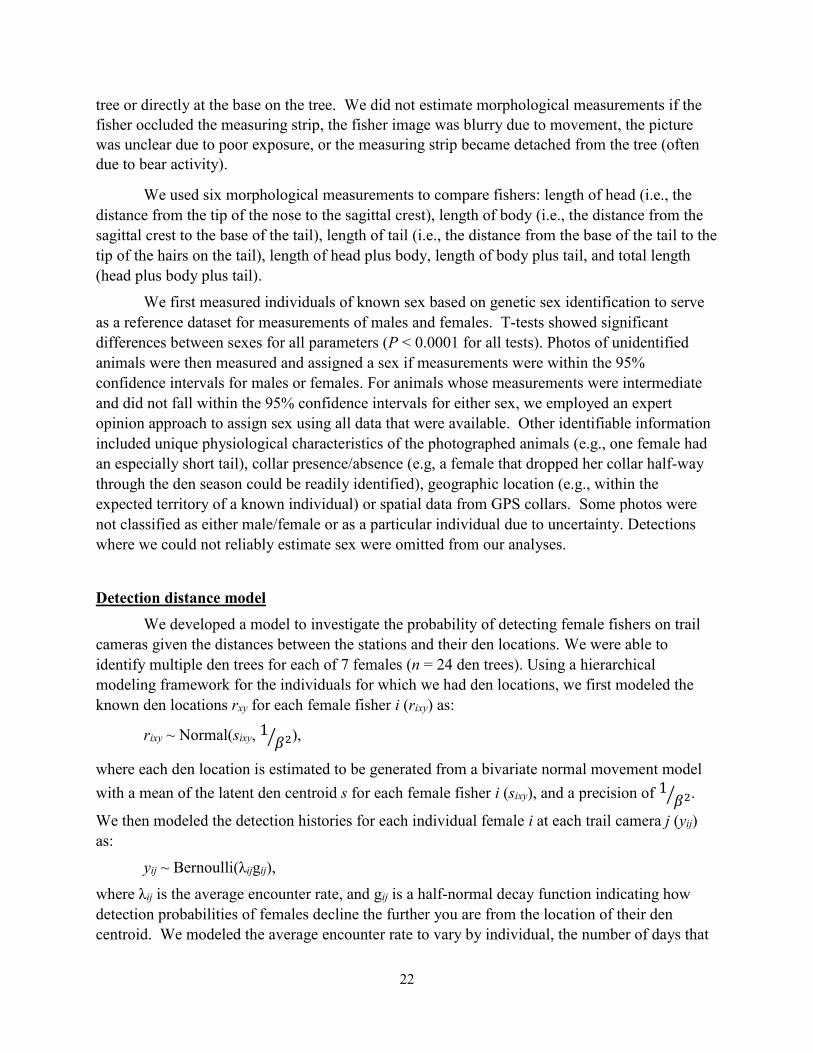
Detection distance model
We developed a model to investigate the probability of detecting female fishers on trail
cameras given the distances between the stations and their den locations. We were able to
identify multiple den trees for each of 7 females (n = 24 den trees). Using a hierarchical
modeling framework for the individuals for which we had den locations, we first modeled the
known den locations rxy for each female fisher i (rixy) as:
rixy ~ Normal(sixy, 1 𝛽2⁄ ),
where each den location is estimated to be generated from a bivariate normal movement model
with a mean of the latent den centroid s for each female fisher i (sixy), and a precision of 1 𝛽2⁄ .
We then modeled the detection histories for each individual female i at each trail camera j (yij)
as:
yij ~ Bernoulli(λijgij),
where λij is the average encounter rate, and gij is a half-normal decay function indicating how
detection probabilities of females decline the further you are from the location of their den
centroid. We modeled the average encounter rate to vary by individual, the number of days that
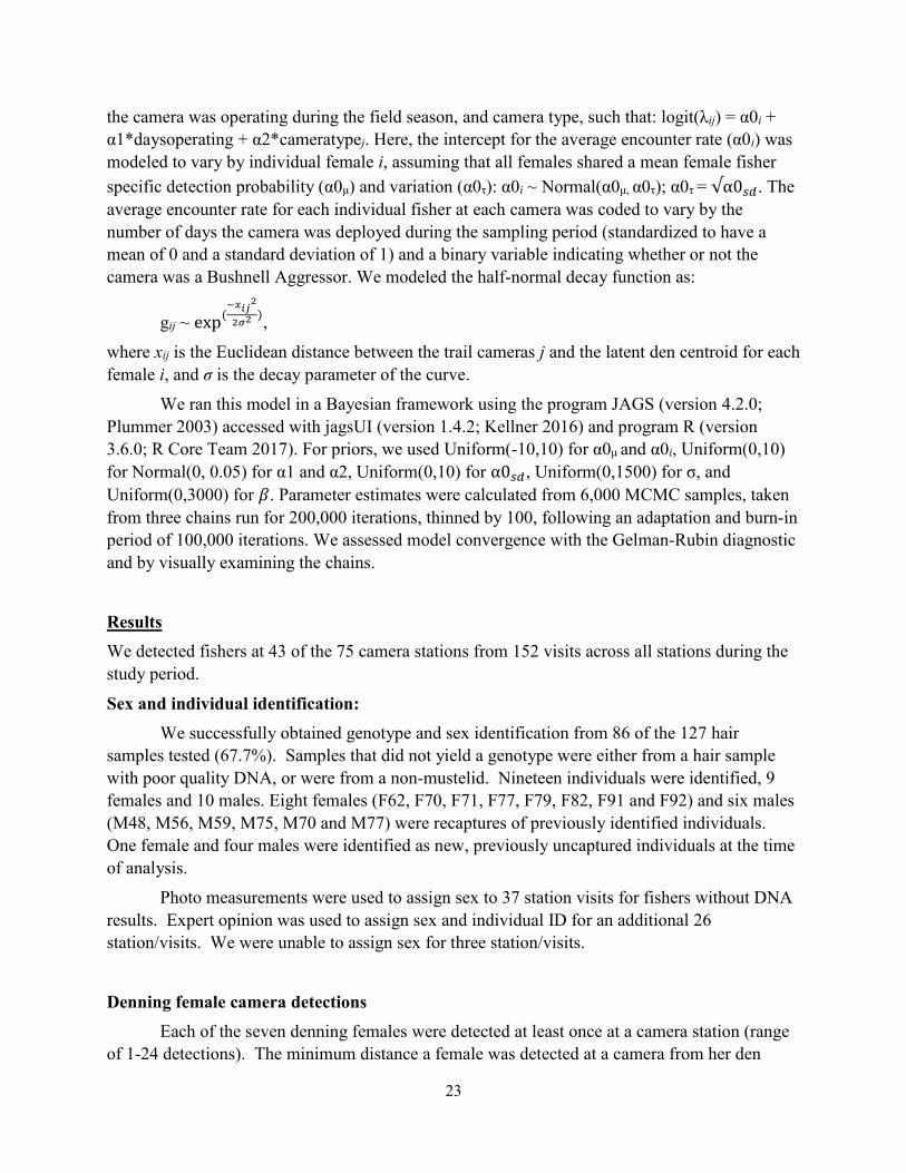
23
the camera was operating during the field season, and camera type, such that: logit(λij) = α0i +
α1*daysoperating + α2*cameratypej. Here, the intercept for the average encounter rate (α0i) was
modeled to vary by individual female i, assuming that all females shared a mean female fisher
specific detection probability (α0μ) and variation (α0τ): α0i ~ Normal(α0μ, α0τ); α0τ = √α0𝑠𝑑. The
average encounter rate for each individual fisher at each camera was coded to vary by the
number of days the camera was deployed during the sampling period (standardized to have a
mean of 0 and a standard deviation of 1) and a binary variable indicating whether or not the
camera was a Bushnell Aggressor. We modeled the half-normal decay function as:
gij ~ exp(−𝑥𝑖𝑗
2
2𝜎2),
where xij is the Euclidean distance between the trail cameras j and the latent den centroid for each
female i, and σ is the decay parameter of the curve.
We ran this model in a Bayesian framework using the program JAGS (version 4.2.0;
Plummer 2003) accessed with jagsUI (version 1.4.2; Kellner 2016) and program R (version
3.6.0; R Core Team 2017). For priors, we used Uniform(-10,10) for α0μ and α0i, Uniform(0,10)
for Normal(0, 0.05) for α1 and α2, Uniform(0,10) for α0𝑠𝑑 , Uniform(0,1500) for σ, and
Uniform(0,3000) for 𝛽. Parameter estimates were calculated from 6,000 MCMC samples, taken
from three chains run for 200,000 iterations, thinned by 100, following an adaptation and burn‐in
period of 100,000 iterations. We assessed model convergence with the Gelman-Rubin diagnostic
and by visually examining the chains.
Results
We detected fishers at 43 of the 75 camera stations from 152 visits across all stations during the
study period.
Sex and individual identification:
We successfully obtained genotype and sex identification from 86 of the 127 hair
samples tested (67.7%). Samples that did not yield a genotype were either from a hair sample
with poor quality DNA, or were from a non-mustelid. Nineteen individuals were identified, 9
females and 10 males. Eight females (F62, F70, F71, F77, F79, F82, F91 and F92) and six males
(M48, M56, M59, M75, M70 and M77) were recaptures of previously identified individuals.
One female and four males were identified as new, previously uncaptured individuals at the time
of analysis.
Photo measurements were used to assign sex to 37 station visits for fishers without DNA
results. Expert opinion was used to assign sex and individual ID for an additional 26
station/visits. We were unable to assign sex for three station/visits.
Denning female camera detections
Each of the seven denning females were detected at least once at a camera station (range
of 1-24 detections). The minimum distance a female was detected at a camera from her den
24
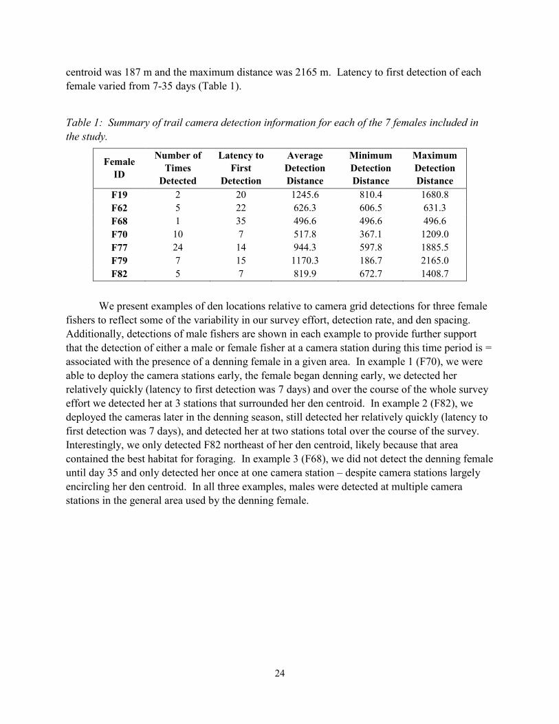
centroid was 187 m and the maximum distance was 2165 m. Latency to first detection of each
female varied from 7-35 days (Table 1).
Table 1: Summary of trail camera detection information for each of the 7 females included in
the study.
Female
ID
Number of
Times
Detected
Latency to
First
Detection
Average
Detection
Distance
Minimum
Detection
Distance
Maximum
Detection
Distance
F19 2 20 1245.6 810.4 1680.8
F62 5 22 626.3 606.5 631.3
F68 1 35 496.6 496.6 496.6
F70 10 7 517.8 367.1 1209.0
F77 24 14 944.3 597.8 1885.5
F79 7 15 1170.3 186.7 2165.0
F82 5 7 819.9 672.7 1408.7
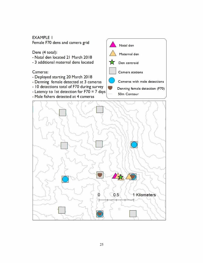
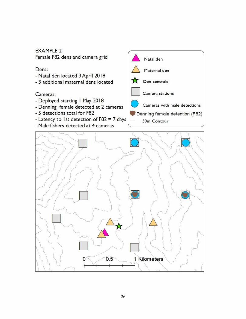
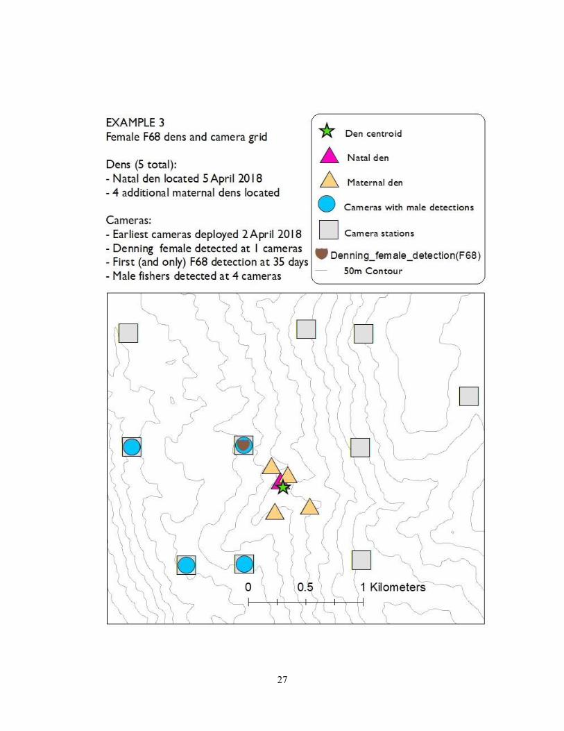
We present examples of den locations relative to camera grid detections for three female
fishers to reflect some of the variability in our survey effort, detection rate, and den spacing.
Additionally, detections of male fishers are shown in each example to provide further support
that the detection of either a male or female fisher at a camera station during this time period is =
associated with the presence of a denning female in a given area. In example 1 (F70), we were
able to deploy the camera stations early, the female began denning early, we detected her
relatively quickly (latency to first detection was 7 days) and over the course of the whole survey
effort we detected her at 3 stations that surrounded her den centroid. In example 2 (F82), we
deployed the cameras later in the denning season, still detected her relatively quickly (latency to
first detection was 7 days), and detected her at two stations total over the course of the survey.
Interestingly, we only detected F82 northeast of her den centroid, likely because that area
contained the best habitat for foraging. In example 3 (F68), we did not detect the denning female
until day 35 and only detected her once at one camera station – despite camera stations largely
encircling her den centroid. In all three examples, males were detected at multiple camera
stations in the general area used by the denning female.
25
26
27
28
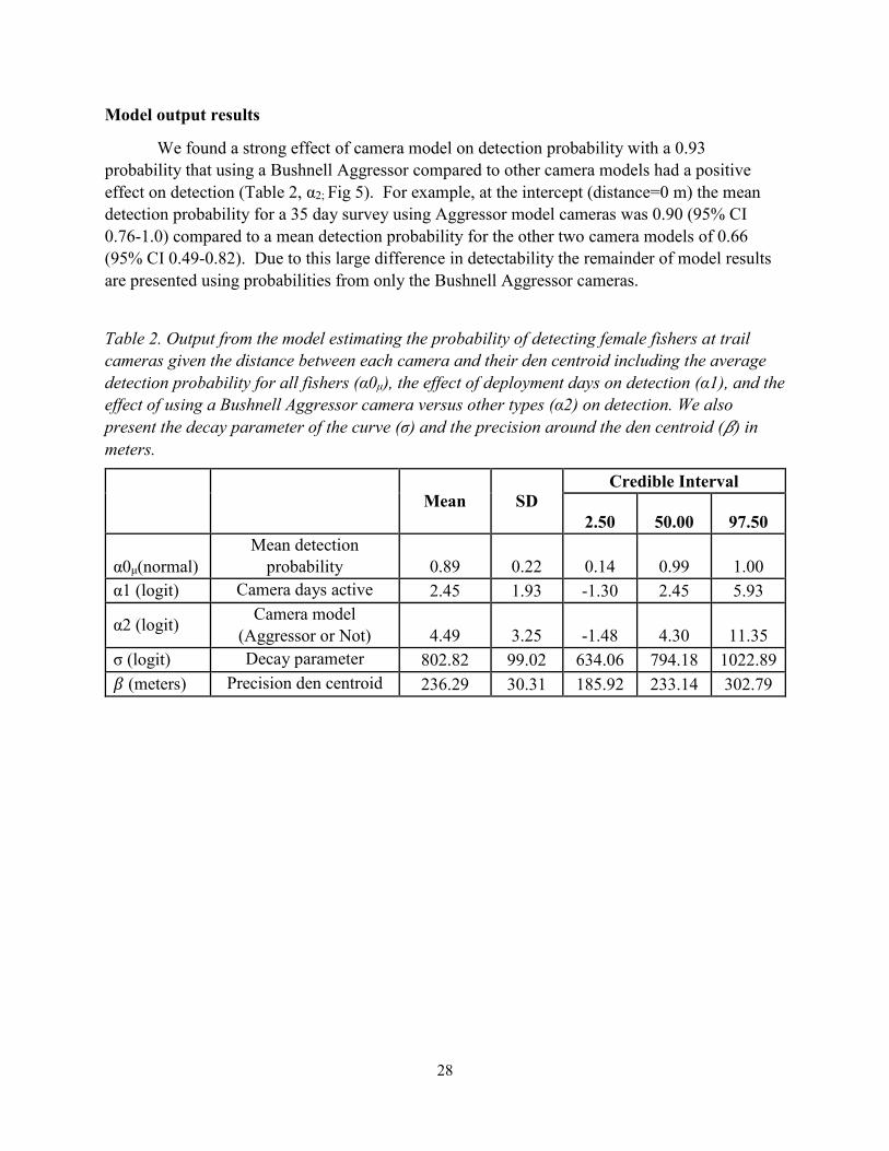
Model output results
We found a strong effect of camera model on detection probability with a 0.93
probability that using a Bushnell Aggressor compared to other camera models had a positive
effect on detection (Table 2, α2; Fig 5). For example, at the intercept (distance=0 m) the mean
detection probability for a 35 day survey using Aggressor model cameras was 0.90 (95% CI
0.76-1.0) compared to a mean detection probability for the other two camera models of 0.66
(95% CI 0.49-0.82). Due to this large difference in detectability the remainder of model results
are presented using probabilities from only the Bushnell Aggressor cameras.
Table 2. Output from the model estimating the probability of detecting female fishers at trail
cameras given the distance between each camera and their den centroid including the average
detection probability for all fishers (α0μ), the effect of deployment days on detection (α1), and the
effect of using a Bushnell Aggressor camera versus other types (α2) on detection. We also
present the decay parameter of the curve (σ) and the precision around the den centroid (𝛽) in
meters.
Mean SD Credible Interval
2.50 50.00 97.50
α0μ(normal)
Mean detection
probability 0.89 0.22 0.14 0.99 1.00
α1 (logit) Camera days active 2.45 1.93 -1.30 2.45 5.93
α2 (logit) Camera model
(Aggressor or Not) 4.49 3.25 -1.48 4.30 11.35
σ (logit) Decay parameter 802.82 99.02 634.06 794.18 1022.89
𝛽 (meters) Precision den centroid 236.29 30.31 185.92 233.14 302.79
29
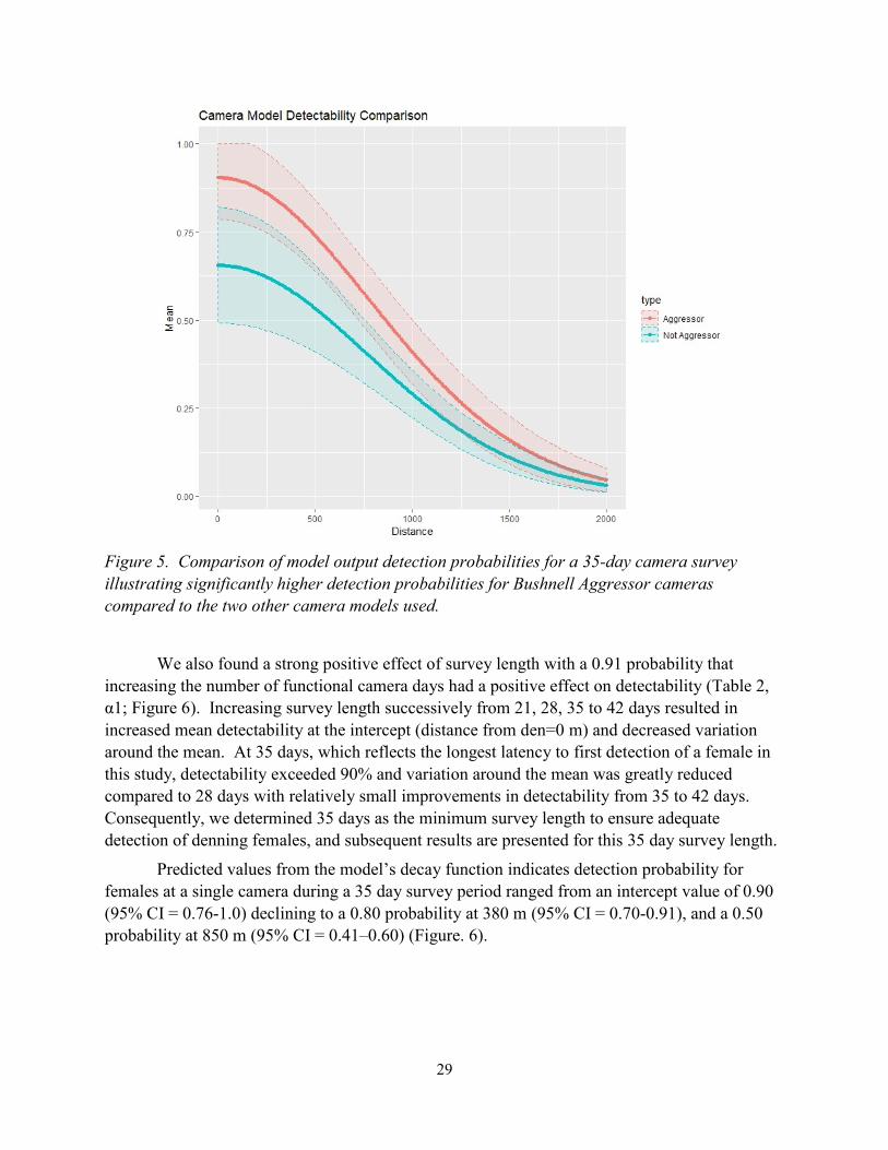
Figure 5. Comparison of model output detection probabilities for a 35-day camera survey
illustrating significantly higher detection probabilities for Bushnell Aggressor cameras
compared to the two other camera models used.
We also found a strong positive effect of survey length with a 0.91 probability that
increasing the number of functional camera days had a positive effect on detectability (Table 2,
α1; Figure 6). Increasing survey length successively from 21, 28, 35 to 42 days resulted in
increased mean detectability at the intercept (distance from den=0 m) and decreased variation
around the mean. At 35 days, which reflects the longest latency to first detection of a female in
this study, detectability exceeded 90% and variation around the mean was greatly reduced
compared to 28 days with relatively small improvements in detectability from 35 to 42 days.
Consequently, we determined 35 days as the minimum survey length to ensure adequate
detection of denning females, and subsequent results are presented for this 35 day survey length.
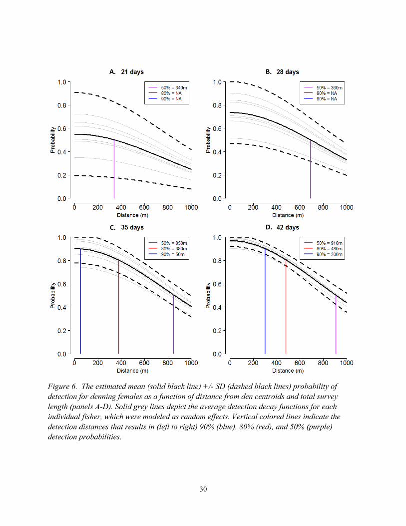
Predicted values from the model’s decay function indicates detection probability for
females at a single camera during a 35 day survey period ranged from an intercept value of 0.90
(95% CI = 0.76-1.0) declining to a 0.80 probability at 380 m (95% CI = 0.70-0.91), and a 0.50
probability at 850 m (95% CI = 0.41–0.60) (Figure. 6).
30
Figure 6. The estimated mean (solid black line) +/- SD (dashed black lines) probability of
detection for denning females as a function of distance from den centroids and total survey
length (panels A-D). Solid grey lines depict the average detection decay functions for each
individual fisher, which were modeled as random effects. Vertical colored lines indicate the
detection distances that results in (left to right) 90% (blue), 80% (red), and 50% (purple)
detection probabilities.
A. B.
C. D.
31
Estimating required camera spacing
We next scaled the model estimated single camera detection probabilities to detectability
for arrays of multiple cameras. Assuming you have d cameras at different distances from a den
center, each with a distance specific detection probability (p), for a fixed number of visits (35
days=5 visits), the overall probability of detecting a species on at least one camera during the
survey (Pd) is estimated as:
Pd = 1- [(1-p1) * (1-p2)… *(1-pd)]
Therefore, to achieve 95% detectability with 2 cameras a single camera detectability of at
least 0.78 per camera is required [0.95=1-(1-0.78)2]; for 4 cameras a single camera detectability
of 0.53 is required [0.95=1-(1-0.53)4], or for 6 cameras a single camera detectability of 0.39
[0.95=1-(1-0.39)6].
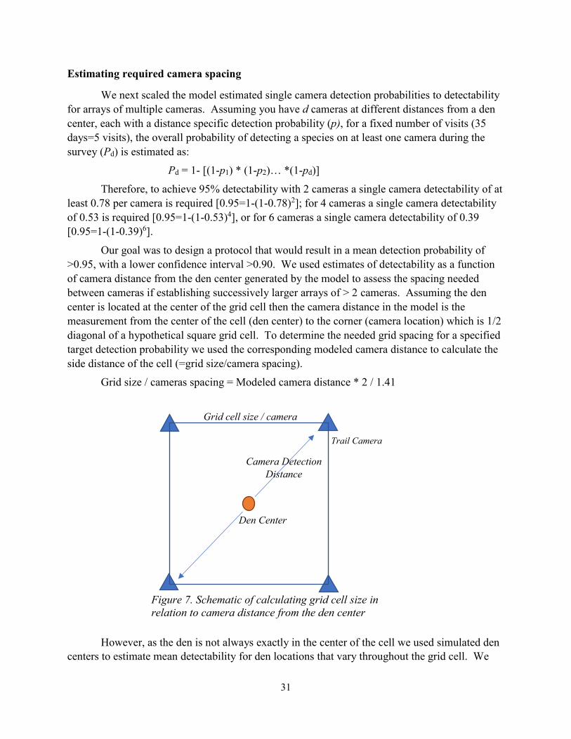
Our goal was to design a protocol that would result in a mean detection probability of
>0.95, with a lower confidence interval >0.90. We used estimates of detectability as a function
of camera distance from the den center generated by the model to assess the spacing needed
between cameras if establishing successively larger arrays of > 2 cameras. Assuming the den
center is located at the center of the grid cell then the camera distance in the model is the
measurement from the center of the cell (den center) to the corner (camera location) which is 1/2
diagonal of a hypothetical square grid cell. To determine the needed grid spacing for a specified
target detection probability we used the corresponding modeled camera distance to calculate the
side distance of the cell (=grid size/camera spacing).
Grid size / cameras spacing = Modeled camera distance * 2 / 1.41
Figure 7. Schematic of calculating grid cell size in
relation to camera distance from the den center
However, as the den is not always exactly in the center of the cell we used simulated den
centers to estimate mean detectability for den locations that vary throughout the grid cell. We
Camera Detection
Distance
Grid cell size / camera
spacing
Den Center
Trail Camera
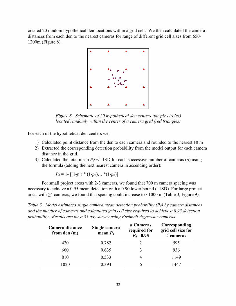
32
created 20 random hypothetical den locations within a grid cell. We then calculated the camera
distances from each den to the nearest cameras for range of different grid cell sizes from 650-
1200m (Figure 8).
Figure 8. Schematic of 20 hypothetical den centers (purple circles)
located randomly within the center of a camera grid (red triangles)
For each of the hypothetical den centers we:
1) Calculated point distance from the den to each camera and rounded to the nearest 10 m
2) Extracted the corresponding detection probability from the model output for each camera
distance in the grid.
3) Calculated the total mean Pd +/- 1SD for each successive number of cameras (d) using
the formula (adding the next nearest camera in ascending order):
Pd = 1- [(1-p1) * (1-p2)… *(1-pd)]
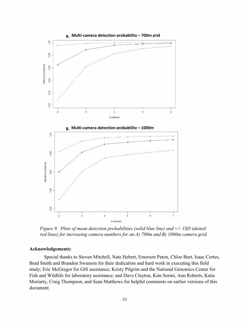
For small project areas with 2-3 cameras, we found that 700 m camera spacing was
necessary to achieve a 0.95 mean detection with a 0.90 lower bound (–1SD). For large project
areas with >4 cameras, we found that spacing could increase to ~1000 m (Table 3, Figure 9).
Table 3. Model estimated single camera mean detection probability (Pd) by camera distances
and the number of cameras and calculated grid cell size required to achieve a 0.95 detection
probability. Results are for a 35 day survey using Bushnell Aggressor cameras.
Camera distance
from den (m)
Single camera
mean Pd
# Cameras
required for
Pd =0.95
Corresponding
grid cell size for
# cameras
420 0.782 2 595
660 0.635 3 936
810 0.533 4 1149
1020 0.394 6 1447
33
Acknowledgements:
Special thanks to Steven Mitchell, Nate Hebert, Emerson Paton, Chloe Burt, Isaac Cortes,
Brad Smith and Brandon Swanson for their dedication and hard work in executing this field
study; Eric McGregor for GIS assistance; Kristy Pilgrim and the National Genomics Center for
Fish and Wildlife for laboratory assistance; and Dave Clayton, Kim Sorini, Ann Roberts, Katie
Moriarty, Craig Thompson, and Sean Matthews for helpful comments on earlier versions of this
document.
Figure 9. Plots of mean detection probabilities (solid blue line) and +/- 1SD (dotted
red lines) for increasing camera numbers for an A) 700m and B) 1000m camera grid.
Multi-camera detection probability – 700m grid
35 days
Multi-camera detection probability – 1000m
grid, 35 days
B.
A.
34
Literature Cited
Basto, M.P., Rodrigues, M., Santos-Reis, M., Bruford, M.W. and Fernandes, C.A., 2010.
Isolation and characterization of 13 tetranucleotide microsatellite loci in the Stone marten
(Martes foina). Conservation Genetics Resources, 2: 17-319.
Burton, A.C., Neilson, E., Moreira, D., Ladle, A., Steenweg, R., Fisher, J.T., Bayne, E. and
Boutin, S., 2015. Wildlife camera trapping: a review and recommendations for linking
surveys to ecological processes. Journal of Applied Ecology, 52: 675-685.
Buskirk, J., K. M. Moriarty, M. A. Linnell, C. M. Kelsey, and B. R. Barry. 2018. Determining
sex of Pacific martens from remote camera data. Conference: International Martes
Symposium. Ashland, Wisconsin.
Dallas J., and S. Piertney. 1998. Microsatellite primers for the Eurasian otter. Molecular Ecology
7: 1248-1251.
Davis C. S., and C. Strobeck. 1998. Isolation, variability, and cross-species amplification of
polymorphic microsatellite loci in the family Mustelidae. Molecular Ecology, 7: 1776-1778.
Duffy A. J., A. Landa, M. O'Connell, C. Stratton, and J. M. Wright. 1998. Four polymorphic
microsatellite in wolverine, Gulo gulo. Animal Genetics, 29: 63-72.
Green, R. E. 2017. Reproductive ecology of the fisher (Pekania pennanti) in the southern Sierra
Nevada: an assessment of reproductive parameters and forest habitat used by denning
females. PhD dissertation, University of California, Davis.
Green, R. E., M. J. Joyce, S. M. Matthews, K. L. Purcell, J.M. Higley, and A. Zalewski. 2017.
Guidelines and techniques for studying the reproductive ecology of wild fishers (Pekania
pennanti), American martens (Martes americana), and other members of the Martes
Complex. Pp. 313–358 in The Martes Complex in the 21st century: ecology and
conservation (A. Zalewski, I. A. Wierzbowska, K. B. Aubry, J. D. S. Birks, D. T.
O’Mahony, and G. Proulx, eds.). Mammal Research Institute, Polish Academy of Sciences,
Bialowieza, Poland.
Green, R. E., K. L. Purcell, C. M. Thompson, D. A. Kelt, and H. U. Wittmer. 2018.
Reproductive parameters of the fisher (Pekania pennanti) in the southern Sierra Nevada,
California. Journal of Mammalogy, 99: 537-553.
Green, R. E., K. L. Purcell, C. M. Thompson, D. A. Kelt, and H. U. Wittmer. 2019. Microsites
and structures used by fishers (Pekania pennanti) in the southern Sierra Nevada: a
comparison of forest elements used for daily resting relative to reproduction. Forest
Ecology and Management, 440: 131-146.
Fleming, M.A., Ostrander, E.A. and Cook, J.A., 1999. Microsatellite markers for American mink
(Mustela vison) and ermine (Mustela erminea). Molecular Ecology, 8: 1352-1355.
Hedmark E., Ø. Flagstad, P. Segerstroem, J. Persson, A. Landa, and H. Ellegren. 2004. DNA-
based individual and sex identification from wolverine (Gulo gulo) faeces and urine.
Conservation Genetics, 5: 405-410.
35
Jordan M. J., J. M. Higley, S. M. Mattews, O. E. Rhodes, M. K. Schwartz, R. H. Barrett, and P.
J. Palsbøll. 2007. Development of 22 new microsatellite loci for fishers (Martes pennanti)
with variability results from across their range. Molecular Ecology Notes 7: 797-801.
Kellner, K. (2016) jagsUI: A wrapper around ‘rjags’ to streamline ‘JAGS’ analyses. R package
version 1.4.2. URL https://cran.r-project.org/package=jagsUI.
Lofroth, E.C., Raley, C.M., Higley, J.M., Truex, R.L., Yaeger, J.S., Lewis, J.C., Happe, P.J.,
Finley, L.L., Naney, R.H., Hale, L.J. and Krause, A.L., 2010. Conservation of fishers
(Martes pennanti) in south-central British Columbia, western Washington, western Oregon,
and California–volume I: conservation assessment. USDI Bureau of Land Management,
Denver, Colorado, USA.
O’Brien, C. J., and R. A. Sweitzer. 2012. Identifying sex of fishers (Martes pennanti) visiting
camera stations in the Sierra National Forest, California. Poster at the Wildlife Society
Western Section Meeting, Sacramento, CA.
Plummer, M. (2003) JAGS: A program for analysis of Bayesian graphical models using Gibbs
sampling. Proceedings of the 3rd International Workshop on Distributed Statistical
Computing. Vienna, Austria.
R Core Team (2019). R: A language and environment for statistical computing. R Foundation for
Statistical Computing, Vienna, Austria. URL https://www.R-project.org/.
Spencer, W., Sawyer, S., Romsos, H.L., Zielinski, W.J., Sweitzer, R.A., Thompson, C.M.,
Purcell, K.L., Clifford, D.L., Cline, L., Safford, H.D., Britting, S.,and Tucker, J.M. 2015.
Southern Sierra Nevada fisher conservation assessment. Conservation Biology Institute, San
Diego, CA.
Spencer, W., Sawyer, S., Romsos, H., Zielinski, W.J., Thompson, C.M. and Britting, S. 2016.
Southern Sierra Nevada Fisher Conservation Strategy. Conservation Biology Institute, San
Diego, CA.
US Fish and Wildlife Service, 2012. Protocol for surveying proposed management activities that
may impact Northern Spotted Owls. February 2, 2011; Revised January 9, 2012.
Vincent, I.R., Farid, A. and Otieno, C.J., 2003. Variability of thirteen microsatellite markers in
American mink (Mustela vison). Canadian Journal of Animal Science, 83: 597-599.
Walker, C.W., Vila, C., Landa, A., Linden, M. and Ellegren, H., 2001. Genetic variation and
population structure in Scandinavian wolverine (Gulo gulo) populations. Molecular
Ecology, 10: 53-63.
Wellington, K., Bottom, C., Merrill, C. and Litvaitis, J.A., 2014. Identifying performance
differences among trail cameras used to monitor forest mammals. Wildlife Society
Bulletin, 38: 634-638.


