
Cash Flow and Budgetary Variance Analysis
BY SHAYNE C. KAVANAGH AND CHRISTOPHER J. SWANSON
TACT ICAL F INANCIAL
MANAGEMENT
Most discussion of financial planning centers on a
budgetary perspective — the revenues and expen-
ditures that occur annually. Also, much attention
has been focused on strategic financial management meth-
ods such as long-term financial planning and priority-based
budgeting. A tactical perspective is especially important
during times of uncertainty: the incidence and behavior of
revenues and expenditures during the course of the year. In
the current environment, public officials can’t wait until
the end of the year to get an accurate picture of financial
position, and the choppy seas of the economy require con-
stant course corrections. The ability to make these timely
alterations guards against having to make more draconian
adjustments later.
Two related techniques can help keep the financial ship of
state on course: cash flow analysis and monthly budget vari-
ance analysis. Cash flow analysis tracks actual income
against outflows of cash to discern patterns, providing insight
into a government’s ability to meet expenditure obligations
without resorting to the use of reserves or short-term debt.
Cash flow can also highlight patterns that might affect
long-range financial position. Variance analysis compares
monthly budgets against actual numbers to highlight devia-
tions between strategy and execution. Variance analysis
can illuminate the beginnings of unsustainable trends and
help the organization manage its budget in a way that is
better aligned with its strategic goals. Variance analysis also
helps track cash by comparing what was expected to happen
October 2009 | Government Finance Review 9
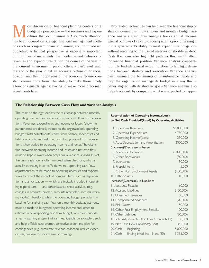
The chart to the right depicts the relationship between monthly
operating revenues and expenditures, and cash flow from opera-
tions. Revenues, expenditures and income or losses (shown in
parentheses) are directly related to the organization’s operating
budget.“Total Adjustments” come from balance sheet asset and
liability accounts, and yield net cash flow provided from opera-
tions when added to operating income and losses.The distinc-
tion between operating income and losses and net cash flow
must be kept in mind when preparing a variance analysis. In fact,
the term cash flow is often misused when describing what is
actually operating income.To derive net operating cash flow,
adjustments must be made to operating revenues and expendi-
tures to reflect the impact of non-cash items such as deprecia-
tion and amortization — which are typically included in operat-
ing expenditures — and other balance sheet activities (e.g.,
changes in accounts payable, accounts receivable, accruals, work-
ing capital).Therefore, while the operating budget provides the
baseline for analyzing cash flow on a monthly basis, adjustments
must be made to budgeted operating income and losses to
estimate a corresponding cash flow budget, which can provide
an early warning system that can help identify unfavorable trends
and help officials take prompt corrective action and plan for
contingencies (e.g., accelerate revenue collection, reduce expen-
ditures, prepare for short-term borrowing).
Reconciliation of Operating Income/(Loss)
to Net Cash Provided/(Used) by Operating Activities
1. Operating Revenues $5,000,0002. Operating Expenditures 4,750,0003. Operating Income/(Loss) 250,0004. Add: Depreciation and Amortization 2000,000
(Increase)/Decrease in Assets5. Accounts Receivable (1000,000)6. Other Receivables (50,000)7. Inventories 30,0008. Prepaid Items 5,0009. Other Post Employment Assets (100,000)
10. Other Assets 10,000Increase/(Decrease) in Liabilities11.Accounts Payable 60,00012. Accrued Liabilities (100,000)13. Unearned Revenues 50,00014. Compensated Absences (20,000)15. Risk Claims 50,00016. Other Post Employment Benefits 100,00017. Other Liabilities (30,000)18.Total Adjustments (Add lines 4 through 17) 105,00019. Net Cash Flow Provided/(Used) 355,00020. Cash — Beginning 5,000,00021. Cash — Ending (Add line 19 and 20) 5,355,000
The Relationship Between Cash Flow and Variance Analysis

10 Government Finance Review | October 2009
versus what actually did.1 Together, cash flow and variance
analysis provide unique tactical insight.
This article describes some of the most useful applications
for cash flow and variance analysis, what a good cash flow
and variance analysis model looks like,
and specific modeling techniques. The
following organizations contributed to
the Government Finance Officers
Association’s research on cash flow and
variance analysis:Prince George’s County,
Maryland; the City of Irvine, California;
and the City of Scottsdale,Arizona.
VALUABLE APPLICATIONS
Investment Management. Investment management is the
most common use of cash flow modeling for local govern-
ments. Cash flow modeling can determine the dollar amount
that the portfolio needs to remain liquid and meet disburse-
ment obligations (generally within a six-month period),
thereby revealing the amount available for investment.
Prince George’s County has found that its cash flow manage-
ment practices have provided comfort that liquidity needs
can be met, thereby providing the confidence to invest over a
longer timeframe than it otherwise might. In 2001, the county
started making investments with maturities that were greater
than one year. This change in tactics
added $10 million in investment income
(government-wide) on an average $750
million investment portfolio (of course,
going long might not offer the same
advantages today).
Sizing Fund Balance. Cash flow and
variance analysis can be used to demon-
strate the need for working capital. The
City of Irvine has found that getting a better handle on
volatility informs reserves requirements. If cash flow analysis
reveals that revenues are very volatile such that cash reserves
may become dangerously low for a period of time (during
revenue low points), this suggests the need for a higher
working capital reserve. At least one rating agency appar-
ently agrees with the city, advocating that a government’s
formal operating reserve policy take into account the
Exhibit 1: Monthly Variance Analysis, Aggregated Chart
The ability to make timely
alterations guards against
having to make more draconian
adjustments later.
14
12
10
8
6
4
2
0July August September October November December January
■ Budget $0.8 $1.3 $4.0 $3.3 $4.9 $7.5 $12.3
■ Actual $0.9 $1.6 $3.0 $3.9 $6.6 $7.5 $10.9
Milli
ons
of D
olla
rs
Total Revenues

government’s cash flow requirements and volatility of
revenues and expenditures.2
Managing Financial Stress. As far as most people are con-cerned,the primary use of cash flow and variance analysis formanaging financial stress is making sure the bills can be paid.It describes where income and disbursements are comingfrom and where they are going. For example, during a recession in the early 1990s, Prince George’s County foundthat summer is traditionally a lean time for revenues and thatshort-term borrowing would be needed to bridge thosemonths.The county’s elected officials did not generally lookfavorably on the prospect of short-term borrowing, but man-agement was able to demonstrate,using its cash flow models,that bridge financing could be a responsible solution for thesummer cash shortage because revenues would return in thefall.The county’s cash flow model also served as the basis forcommunication with rating agencies. The county was able to maintain its bond rating, despite short-term borrowing, by
illustrating how the borrowing fit into a cogent financial strat-egy and by using the model to identify and explain variancesfrom its financial strategy.
Cash flow and variance analysis is not just of value in a cash
shortage. It foreshadows unfavorable trends that will develop
into problems later in the year, thereby enabling better strate-
gic management for both revenues and expenditures. For
example, the City of Irvine used variance analysis to discover
that its revenue income was fluctuating from monthly expec-
tations (which were modeled on detailed month-over-month
comparisons from previous years).This prompted the city to
analyze its actual revenues in more detail, discover the root
causes to the variances, and then adjust the city’s short- and
long-term forecasts accordingly. (Exhibit 1 shows a consoli-
dated view of all revenues compared with monthly budgets
for a hypothetical municipality. Exhibit 2 presents monthly
variances by revenue type.)
October 2009 | Government Finance Review 11
Exhibit 2: Montly Variance Analysis, Detailed TableFiscal Year 2008-2009 FY 2007-2008
All Revenues Annual Budget YTD Budget YTD Actual Favorable/ Percent YTD Change from PercentSources Adopted Adjusted Jan 2009 Jan 2009 (Unfavorable) Prior Year Prior Year
Sales Tax $27,941,250 $27,941,250 $11,957,965 $10,473,760 $(1,484,204) -12% $12,563,400 $(2,089,640) -17%
Property Tax 21,708,500 21,708,500 11,423,198 11,417,680 (5,518) 0% 11,059,684 357,996 3%
Hotel Tax 5,315,000 5,315,000 2,591,568 2,079,686 (511,883) -20% 2,240,279 (160,593) -7%
Franchise Tax 3,717,500 3,717,500 532,537 808,138 275,601 52% 445,022 363,116 82%
Community Services Fees 3,527,895 3,477,951 2,087,354 2,253,237 165,883 8% 1,989,651 263,586 13%
Utility Users Tax 2,218,500 2,218,500 1,119,272 1,196,681 77,410 7% 1,169,846 26,835 2%
Fines & Forfeitures 1,066,000 1,066,000 518,174 488,260 (29,914) -6% 601,946 (113,686) -19%
Documentary Transfer Tax 800,000 800,000 357,661 268,934 (88,727) -25% 308,780 (39,845) -13%
Motor Vehicle In-Lieu Revenues 496,500 496,500 222,266 162,519 (59,747) -27% 210,300 (47,781) -23%
Licenses & Permits 813,000 813,000 415,991 441,752 25,761 6% 493,634 (51,882) -11%
Miscellaneous Revenues 352,573 352,573 221,102 137,922 (83,182) -38% 285,724 (147,802) -52%
Revenues from Other Sources 875,991 958,428 531,559 309,537 (222,023) -42% 299,041 10,496 4%
Fees for Services 597,302 597,302 325,008 369,924 44,916 14% 343,115 26,808 8%
Community Development Fees 112,500 112,500 63,573 53,815 (9,758) -15% 67,704 (13,890) -21%
Public Works Development Fees 34,660 34,660 20,194 2,493 (17,701) -88% 18,111 (15,618) -86%
Total Operating Revenue 69,577,170 69,609,663 32,387,424 30,464,337 (1,923,087) -6% 32,096,238 (1,631,901) -5%
Transfers In 4,448,093 8,671,903 1,726,600 3,954,754 2,228,153 129% (1,631,901)
Total Revenues & Sources $74,025,262 $78,281,561 $34,114,024 $34,419,090 $305,066 1% $32,096,238 $2,322,852 7%

12 Government Finance Review | October 2009
Cash flow and variance monitoring can also help stabilize
tax and fee changes, which is important to constituents who
are also contending with the recession.The City of Scottsdale
continually monitors its tax and fee performance against
expenditures on a monthly basis.3 For instance, one of the
city’s goals is to keep its water usage rates stable, with incre-
mental increases from year to year that users can afford
instead of less frequent but larger increases. By monitoring
the extent to which water revenues are meeting current
expenses and obligations, while simultaneously building
up funds for future infrastructure projects, the city can avoid
rate spikes and achieve long-run rate stability.
Many states are experiencing severe financial distress, andthe effects are trickling down to local governments.Cash flowand variance analysis can be used to model legislative initiatives and proposed changes to financial plans. For example, a new law might defer receipt of revenues or evenreduce them outright. In Scottsdale, the state legislaturepassed legislation to reduce the property tax assessment ratio for commercial property by 1 percent per year over fiveyears. The city built cash models to see how this tax reduc-tion would affect the availability of funding to provide a stable portfolio of essential services throughout the five-yearprojection period.
Modeling and monitoring salary variances for attrition ordelayed recruitments helps Scottsdale develop more accurateassumptions for position vacancies. The city is able to makebetter long-term forecasts of salary expenditures and to betterestimate the vacancy savings in its budget.The potential sav-ings from position vacancies is significant, so it is critical toestimate them as accurately as possible.
Exhibit 3: Converting Annual Budgets into Monthly Estimates

As a final example, Scottsdale uses cash flow and variance
analysis for capital improvement projects that are in progress
to determine the completion dates of projects that will affect
operations (e.g., hiring, utilities).The timing of when a partic-
ular project will be completed,such as a fire station or a park,
needs to be evaluated against the cost of facility utilities,
maintenance, and new staffing costs.These supporting activi-
ties must be initiated when required at the project’s comple-
tion and must also be affordable within a balanced budget
plan. This area of capital improvement project work-in-
progress analysis is also critical to properly timing and sizing
debt issuances and pay-as-you-go funding for capital projects.
Communications and Exercise of Financial Leader-ship. For people who do not have a financial background,
cash is potentially an easier concept to understand than
accrual information.A more intuitive presentation of financial
data creates a better understanding of the organization’s
financial position and better credibility for the finance officer,
which helps the finance officer in leading financial strategies.
For example, Irvine uses its analysis to help the City Council
better monitor available funds for projects outside of the city’s
strategic business plan.This has helped restrain the tendency
found in any political environment to add special projects
beyond those originally contemplated in the budget. Irvine
has also found that departments are more apt to use the city’s
analysis to communicate to relevant boards and the public,
thereby infusing financial information into decentralized
decision making.
ANATOMY OF CASH FLOW AND VARIANCE ANALYSIS MODEL
Foremost, a model breaks revenues and expenditures into
meaningful categories. For example, inflows include receipts
such as property taxes, utility payments, user fees, and invest-
ment income and maturities.Maturities include all items held
in investments that will mature during the forecast timeframe.
A number of factors should be kept in mind when developing
the cash flow and variance analysis model:
■ Be Conservative. Cash position is hard to change on
short notice, and surprises are not uncommon.
October 2009 | Government Finance Review 13
Exhibit 4: Cumulative Cash Flow
50
40
30
20
10
0
-10
-20
-30
Milli
ons
of D
olla
rs
Lowest Cash Balance
■ Net Monthly Cash ■ Cash Balance
July Sept. Nov. Jan. March May July Sept. Nov. Jan. March May July Sept. Nov.
2007 2008 2009

14 Government Finance Review | October 2009
■ Incorporate Historical Data. Historical data is crucial
for analyzing the month-to-month pattern that will be
reflected in the model. Typically, two to three years of
historical data can provide an adequate base of informa-
tion, though up to five years is ideal. Keep in mind that
new revenue sources with no historical track record will
be added, and economic dislocation can reduce the
predictive value of historical data. Exhibit 3 illustrates
an example of techniques used for converting annual
budgets into monthly estimates.
■ Include a Way to Document or Footnote ImportantAssumptions or Historical Information.4 These notes
clarify the logic of the model and make it more accessi-
ble to users, and they can also be used to highlight points
during the year when the forecast should be revisited —
if, for example, new and valuable information on antici-
pated property tax receipts becomes available three
months into the fiscal year. In Microsoft Excel, the cell
“comments” feature can be used to add and store such
notes.
■ Divide Sources and Uses into the Predictable and theVolatile. The incidence of predictable expenditures such
as salaries and benefits can be analyzed using historical
experience. Expert judgment can be focused on the more
volatile items.
■ Engage Operating Departments. Ideally, operating
departments will be involved in developing reasonable
expectations for when planned expenditures will occur
during the year. However, Prince George’s County has
found that departments are accustomed to building budg-
ets for a year-long period and may find it difficult to make
the switch to monthly perspective — as such, their broad
input on a cash flow and variance model may not pro-
vide as much useful information as it could. Instead, it
Exhibit 5: Cash Uses and Sources
45
40
35
30
25
20
15
10
5
0
Milli
ons
of D
olla
rs
■■■ Uses – Actual ■■ Uses – Forecast
■■■ Sources – Actual ■■ Sources – Forecast
July Sept. Nov. Jan. March May July Sept. Nov. Jan. March May July Sept. Nov.
2007 2008 2009

might be more profitable to focus operating department
input on helping finance offices sharpen their forecasts
for unpredictable or non-recurring events such as capital
projects and grants. During the year, departments should
explain variances from the plan and find root causes of
anomalies.
MODELING AND ANALYSIS
There are a number of ways in which cash flow and vari-
ance analysis can contribute a unique perspective to finan-
cial analysis. Below are some of the most important.
Analyze Special Situations. Modeling can help recog-
nize the issues and situations that influence the organiza-
tion’s cash position. Diagnosing these items can lead to
strategies for cash management techniques such as collect-
ing receipts as soon as possible and managing disburse-
ments judiciously — a good example is Scottsdale’s analysis
of capital project spending patterns to better align financing
with the incidence of expenditures.Finance officers can use
their expertise to decide what issues might provide most
management benefit in their own organization.
Improve Forecasting. The cash flow curve from past
years can be used to predict the same general pattern going
forward. This knowledge will help with financial strategy
development, such as Prince George’s County’s experience
with knowing that lean summer revenues might lead to
a need for bridge financing. In addition, variance analysis
can help users recognize emerging trends that might suggest
a change to the forecast. This information should be used
to refine annual forecasts and, ideally, to create an
adaptable system of monthly rolling forecasts, like the cities
of Irvine and Scottsdale have done. Exhibits 4 and 5 show
examples of cash flow curves and how they reveal trends
across multiple years.
Analyze the Organization’s Financial Position. Cash
flow and variance analysis can introduce a number of ana-
lytical perspectives on the organization’s current financial
position.
■ Budget versus Actual. How does the monthly budget
compare to actual experience? The power of this tech-
nique depends on using an appropriate formula to dis-
tribute the budget over the year.5
■ Year over Year Comparisons. Experience from the
current month can be compared to the same month last
year. Is there a logical explanation for any variance? Is
the reason documented in footnotes in the analytical
model?
■ Year versus Year Comparisons. Comparing the cash
flow curve of the current year to those of previous years
can provide a big-picture perspective on possible
structural changes that may be occurring in government
finances.
■ Cash Flow and Accumulated Cash. Analyzing this area
shows how cash flow is expected to affect reserves. Since
reserves are important to many elected officials, this type
of analysis can resonate with them.
■ Sources of Cash. Maintaining historical revenue data
provides a basis for analyzing trends in cash sources that
may affect future revenue trends.
October 2009 | Government Finance Review 15

16 Government Finance Review | October 2009
CONCLUSION
Cash flow and variance analysis provides tactical insight
into financial position. It can reveal if the implementation
plan for long-term strategies, as expressed through the
budget, is proceeding as anticipated. It can indicate the need
for updates to long-range forecasts. It can provide special
analysis of and perspective on a variety of operational issues.
This kind of tactical financial insight is essential during the
current environment of instability. It helps ensure that
essential services can be provided consistently and that long-
term strategies can stay on track despite short-term volatility. ❙
Notes
1.Budgets often use a cash or cash plus encumbrances basis of accounting,which then makes monthly variance analysis very compatible with cashflow analysis. If the budget is accrual based, then adjustments must bemade to the budget numbers by adding or subtracting non-cash account-ing components.
2.“Financial Management Assessment,”a white paper from Standard andPoor’s, 2006.
3.The Scottsdale examples were adapted from a GFOA white paper by CraigClifford,“An Introduction to Cash Flow Planning and Long-RangeFinancial Planning,”available at http://www.gfoa.org/downloads/CashFlowAnalysis_Scottsdale.pdf.
4.Richard S. Linzer,Anna O. Linzer, Cash Flow Strategies: Innovation inNonprofit Financial Management. (Jossey-Bass: San Francisco) 2007.
5.For distribution techniques, see Christopher J. Swanson and Shayne C.Kavanagh,“Identifying Shortfalls:The Importance of Cash Flow Analysis in Times of Fiscal Stress,”Government Finance Review,April 2009.
SHAYNE C.KAVANAGH is a senior manager in the GFOA’s Research
and Consulting Center in Chicago, Illinois. He can be reached at ska-
[email protected]. CHRISTOPHER J. SWANSON is the founder of
Government Finance Research Group (GFRG), a financial manage-
ment consulting firm specializing in financial planning, cost analysis,
econometric modeling, benchmarking and optimization modeling for
local governments throughout the United States. GFRG designed
and developed the MuniCast interactive financial forecasting model.
Swanson can be contacted at 949-412-6078 or [email protected].
The authors would like to acknowledge the following people for their valuable contributions to this article:■ Kathryn Hewitt, cash and investment manager,
Prince George’s County,Maryland■ Ken Brown,budget officer,City of Irvine,California■ Dave Tungate,manager of budget and business
planning,City of Irvine,California■ Craig Clifford,chief financial officer,City of Scottsdale,
Arizona
Government Finance Officers Association
Capital Project Planning and Evaluation
Expanding the Role of the Finance Officer
JOSEPH P. CASEY AND
MICHAEL J. MUCHA, EDITORS
VOLUME
SERIES
BUDGETING
GFOA
Putting RecommendedBudget Practices into Action
VOLUME
A well prepared capital budget is necessary for successfully planning, funding, and implementing
capital projects, but the process of recognizing capital needs and the creation of a capital plan occurs
long before the development of the annual budget. Finance officers have an opportunity to contribute
valuable insight at all stages in the capital planning process and help local governments make capital
project investments that align with long-term service goals, objectives, and strategies.
With Capital Project Planning and Evaluation: Expanding the Role of the Finance Officer, the GFOA
takes a practical approach to capital project planning. Focusing on common essential projects for
small and mid-size local governments, this eighth volume of the GFOA Budgeting Series provides
finance officers enough information to become “educated consumers” of capital projects and to
become active participants in the capital planning and evaluation process, including needs assess-
ment, project planning, project evaluation, and project implementation.
A New Budgeting Series Book
Government Finance Officers Association


