
Tax Cuts for Whom?Heterogeneous Effects of Income Tax Changes on
Growth & Employment
Owen Zidar
University of California, Berkeley
All UC Group - Huntington Library Conference
April 6, 2013
1

Variation in Tax Policy & Structure of Income Tax Changes
−2
02
−2
02
0 50 100 0 50 100
1982 1991
1993 2003
Avera
ge C
hange in T
ax L
iabili
ty a
s S
hare
of A
GI
AGI PercentileGraphs by Year
2

Research Questions
How does the composition of income tax changes affect subsequent output& employment?
Do tax cuts for high income taxpayers generate more employment &output growth than equivalently sized tax cuts for low and moderateincome taxpayers?
If so, why?
3

Overview
1 Theoretical Framework: Redistribution from savers toconstrained/less patient borrowers
2 Empirical Approach:National: Romer & Romer AER 2010 disaggregated by income groupRegional: Bartik approach
3 Data: Historical returns & counterfactuals from NBER TAXSIM
4 Results: Tax cuts for those with high incomes lead to substantiallyless employment growth and economic activity than similarly sized taxcuts for those with low and moderate incomes
Aggregate consumption, particularly durable consumption, andinvestment tend to increase more strongly after bottom 90% gets taxcutsWeak to nonexistent relationship between tax cuts for the top 10% andemployment growth
4

Motivation
Why study the impacts of these tax changes and how they varyover the income distribution?
Empirical importance of heterogeneity in effects of fiscal policy [e.g.Mertens & Ravn AER forthcoming]
Optimal stimulus design
Effects of ending the Bush tax cuts for certain income groups
Effects of mass refinancing1
But Little direct evidence. Likely due to empirical issues: endogeneity,simultaneity, and observability
1Or any other modestly sized redistributive policies at a business cyclefrequency
5

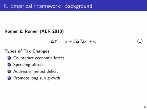
II. Empirical Framework: Background
Romer & Romer (AER 2010)
∆Yt = α + β∆Taxt + εt (1)
Types of Tax Changes
1 Counteract economic forces
2 Spending offsets
3 Address inherited deficit
4 Promote long run growth
6

II. Empirical Framework: Background
Romer & Romer (AER 2010)
∆Yt = α + β∆Taxt + εt (1)
Types of Tax Changes
1 Counteract economic forces
2 Spending offsets
3 Address inherited deficit
4 Promote long run growth
6
II. Empirical Framework: Background
Romer & Romer (AER 2010)
∆Yt = α + β∆Taxt + εt (1)
Types of Tax Changes
1 Counteract economic forces
2 Spending offsets
3 Address inherited deficit
4 Promote long run growth
6

Empirical Framework: (1) Narrative Approach
Output growth & exogenous tax changes for different income groups
GrowthY ,t =β0
+ βB90,0(∆TaxB90,t) + βT 10,0(∆TaxT 10,t) + βNON,0(∆TaxNON,t)︸ ︷︷ ︸=b0∆Taxt
+...
+ βB90,m(∆TaxB90,m) + βT 10,m(∆TaxT 10,m) + βNON,m(∆TaxNON,m)︸ ︷︷ ︸=bm∆Taxt−m
+ Xtλ+ εt
∆TaxB90 and ∆TaxT 10 are changes in income and payroll taxes as a share ofGDP for the bottom 90% and top 10% respectively
Xt is a vector of controls such as lagged GDP growth, government transfers,etc.
Assume Cov(∆Taxg ,t , εt) = 0 ∀g ∈ (BOT90,TOP10,NONINCOME )following Romer & Romer AER 2010
Frisch Waugh
7

Empirical Framework: (2) Bartik Approach
Overview of Bartik approach
Idea: Auto shock on employment in Detroit vs. Denver
Labor literature: Bartik (1991), Card (1992), Katz & Murphy(1992), Moretti (2004)
Implementation: When national tax policy affects high incometaxpayers, states with large shares of high income taxpayers will facelarger shocks
Test: If high income tax cuts have substantial effects, CT and NJshould grow faster following national high income tax cuts
Value: Provides additional identifying variation2
2Within & across state variation. Avoids national concerns: fed & trends8

Data: Constructing tax changes
Tax Change Measure is a function of three things:
1 Income and deductions from year prior to an exogenous tax change3
2 Old tax schedule
3 New tax schedule
3Preliminary tests suggest that results are robust to using two year lags andvarious inflation adjustments
9

Data: Constructing tax changes
Example: 1993 Omnibus Budget Reconciliation Act
10

Data: Constructing tax changes
I do this calculation for entire sample of NBER returns−
1000
01000
2000
Change in T
ax L
iabili
ty
0 50000 100000 150000 200000 250000Adjusted Gross Income
11

Historical Income & Payoll Tax Changes by AGI Quintile
−.6
−.4
−.2
0.2
.4P
erc
ent of G
DP
1960 1970 1980 1990 2000 2010Year
Tax Change: Bottom 20% Tax Change: 21−40%
Tax Change: 41−60% Tax Change: 61−80%
Tax Change: Top 20%
12

Results Overview
National Data:
1 Output and Employment growth
2 Mechanisms: Consumption and Investment
State Data:
1 Similar specification at state-level
2 Effects across the income distribution
13
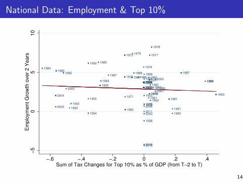
National Data: Employment & Top 10%
1950
1951
19521953
1954
1955
1956
1957
1958
1959
1960
19611962
1963
1964
19651966
19671968
1969
1970
1971
1972
1973
1974
1975
1976
1977
1978
1979
1980
1981
19821983
1984
1985
1986
19871988
1989
1990
1991
1992
1993
19941995
1996
19971998
1999
2000
2001
2002
2003
2004
2005
2006
2007
2008
20092010
2011
−5
05
10
Em
plo
ym
ent G
row
th o
ver
2 Y
ears
−.6 −.4 −.2 0 .2 .4Sum of Tax Changes for Top 10% as % of GDP (from T−2 to T)
14

National Data: Employment & Bottom 90%
1950
1951
19521953
1954
1955
1956
1957
1958
1959
1960
19611962
1963
1964
19651966
19671968
1969
1970
1971
1972
1973
1974
1975
1976
1977
1978
1979
1980
1981
19821983
1984
1985
1986
1987 1988
1989
1990
1991
1992
1993
19941995
1996
19971998
1999
2000
2001
2002
2003
2004
2005
2006
2007
2008
20092010
2011
−5
05
10
Em
plo
ym
ent G
row
th o
ver
2 Y
ears
−1 −.5 0 .5Sum of Tax Changes for Bottom 90% as % of GDP (from T−2 to T)
15

16

State Data: Employment & Top 10%
−10
−5
05
10
Sta
te E
mplo
ym
ent G
row
th
−1 −.5 0 .5 1Sum of Tax Changes for Residents in Top 10% as % of GDP (from T−2 to T)
17

State Data: Employment & Bottom 90%
−10
−5
05
10
Sta
te E
mplo
ym
ent G
row
th
−1.5 −1 −.5 0 .5Sum of Tax Changes for Residents in Bot. 90% as % of GDP (from T−2 to T)
18

Dependent Variable GrowthE,s(1) (2) (3) (4) (5)
∆TaxBot90,s,t 1.1 0.5 -1.1 -0.9 -0.8(1.2) (0.9) (1.0) (0.8) (0.7)
∆TaxBot90,s,t−1 -2.7* -3.2** -1.6** -2.2*** -1.4**(1.5) (1.2) (0.7) (0.7) (0.6)
∆TaxBot90,s,t−2 -1.7 -2.1** 0.5 0.1 -0.3(1.5) (0.9) (0.6) (0.7) (0.6)
∆TaxTop10,s,t 0.2 0.0 -0.1 -0.2 -0.3(0.4) (0.4) (0.2) (0.2) (0.3)
∆TaxTop10,s,t−1 -0.1 -0.2 -0.4 -0.2 -0.2(0.4) (0.3) (0.2) (0.2) (0.3)
∆TaxTop10,s,t−2 -0.2 -0.2 -0.1 0.0 -0.0(0.3) (0.2) (0.2) (0.2) (0.2)
Constant -0.1 -0.3 0.4 -0.2 -2.6**(0.6) (0.6) (0.3) (0.9) (1.2)
State & Year Fixed Effects N Y Y Y YControl for GrowthE lags N N Y Y YControl for GovTransPERCAP,s,t & lags N N N Y YControl for EPOPs,t N N N N YControl for TotalTaxPERCAP,s,t & growth N N N N YControl for squared and cubic lags N N N N YObservations 1,297 1,297 1,247 1,297 1,297R-squared 0.551 0.691 0.810 0.830 0.872Bottom90 Tax Change: βt + βt−1 + βt−2 -3.318 -4.746* -2.189 -2.937* -2.592**t-stat -0.854 -1.873 -1.378 -1.959 -2.433p-val 0.397 0.0670 0.175 0.0558 0.0187Top10 Tax Change: βt + βt−1 + βt−2 -0.164 -0.443 -0.633* -0.416 -0.481*t-stat -0.184 -0.589 -1.792 -1.176 -1.720p-val 0.855 0.558 0.0793 0.245 0.0917
Notes: All results are weighted by state population. Robust standard errors clustered by state are in parentheses. *** p<0.01,** p<0.05, * p<0.1.
19

Effects for more income groups than Bottom 90 & Top 10
How does effect β vary over the income groups?
A second order approximation of the β(g) function
β(g) = θ0 + θ1g + θ2g2
Plug into estimating equation
GrowthY ,t = α + β1∆τ1,t + β2∆τ2,t + ...+ β10∆τ10,t + X̃t λ̃+ ε̃t
GrowthY ,t = α + (θ0 + θ1 + θ2)∆τ1,t + (θ0 + θ12 + θ222)∆τ2,t + ...+ X̃t λ̃+ ε̃t
GrowthY ,t = α + θ0
(10∑
g=1
∆τg ,t
)+ θ1
(10∑
g=1
g ×∆τg ,t
)+ θ2
(10∑
g=1
g2 ×∆τg ,t
)+ X̃t λ̃+ ε̃t
20

Aggregate Effects Across the Income Distribution
1 2 3 4 5 6 7 8 9 10−8
−6
−4
−2
0
AGI Decile
Em
plo
ym
ent
Gro
wth
This figure shows the third order approximation of the β(g) function, i.e., θ̂1g + θ̂2g2 + θ̂3g3
21

Conclusion
Summary
1 Construct a new measure of income tax changes
2 Show substantial heterogeneity in effects of fiscal policy
3 Find stimulative effect of income tax cuts are largely from bottom90% and empirical link between employment growth and tax changesfor upper income earners seems weak to negligible
4 Suggest letting Bush tax cuts expire for $250K won’t have substantialemployment consequences over the business cycle
22


