|
JVL PUBLICATION 80-54
(_ASA-C.'.-I_35u_) IEC6,_I_OkS FO_ _EASORING NdU-3JJ17A_nL_AL '[lff,_':SOE PULSA_ Si_bAi-3 1: DS_
udSEEVArlOtiS Fit03 19o_i TO 1980 (Jet
_ropuisioxL Lab.) bd p dC hO5/,3f A01 gucld-_
CSCL 03A G3/89 28701
Techniques for Measuring ArrivalTimes of Fulsar Signals I: DSN
, Observations from 1968 to 1980
G S DownsP E Reichley
:,- August 15, 1980
;, National Aeronautics andSpace A Jministration
v
Jet Propulsion LaboratoryCalifornia Institute of TechnologyPasad ,ma, California
1
1980024809
https://ntrs.nasa.gov/search.jsp?R=19800024809 2018-07-08T18:07:21+00:00Z
JPL PUBLICATION 80-54
Techniques for Measuring ArrivalTimes of Pulsar Signals I: DSNObservations from 1968 to 1980
G.S. DownsP.E. Reichley
August 15, 1980
Natronal Aeronautics andB;_ce Admin=,_tration
Jet Propulsion LaboratoryCalifornia Institute of TechnologyPasadena, California
+
..i
1980024809-002

ABSTRACT
Natural radio emissions from pulsating radio sources (pulsars) have
been detect_,d ;it Goldstone on a regular basis since 1968. Scientific
analysis of these signals has stimulated ideas of traversing the inter-
planetary medium and beyond, to the "home" of comets, using these natural
beacons as navigation aids. Therefore, the techniques used in the ground-
based ob.qerv:ttit,ns of pulsars are described here in the required detail,
many of !llem bt, ing directly applicable in a navigation scheme. The
arrival times ,,f '.he pulses intercepting Earth are measured at time
intervals w_rying frem a few days to a few months. Low-noise, ,_ide-band
receivers, unique to the stations of NASA's Deep Space Network, amplify
signals intercepted by the 26-m, and 34-m, and 64-m antennas at Goldstone
and in Spain. Digital recordings of total received signal power versus
time are cro._s correlated with the appropriate pulse template, thereby
providing an estimate of the pulse arrival, time relative to the station
clock. Corrections are applied to the station clock to obtain arrival
times relative to ephemeris time. Drifts in phase encountered during
signal integration are removed. The arrival times are then referred to
the barycenter of the solar system for scientific studies, and to the
geocenter for export to other investigators.
PRECEDINGPAGE L'!.A[:.: XOT._'_.-...._;"
iii
1980024809-003

CONTENTS
I. I NTROIIICT I ON 1
I I. DATA COLLECTION 5
A. RECEIVING) DETECTION AND RECORDING 5
B. THE SYSTEM CONFIGURATION CODES 8
C. EFFECTS OF RECEIVER PARAMETERS ON THE ARRIVAL TIME --- 17
l I I. EDITING AND COLLATING 21
A. EDITING TIlE DATA 2i
B. COLLATING THE DATA 2 3
IV. PULSE-SHAPE TEMPLATES 24
A. CORRELATION WIT..'{ A TRIANGLE 25
B. CORRELATION WITH THE TRUE TEMPLATE ..................... 27
C. SUBTRACTION OF THE BACKGROUND 29
D. TIIE TI'MPLATES 30
E. TEMPLATE SMOOTHING j]
F. CENTRAL SPIKES 46
G. DEFINING THE ZERO LEVEl. 46
V. ESTIMATING THE PULSE ARRIVAL TIME 48
A. TIlE CORRELATION PROCESS 48
B. ESTIMATING THE DELAY 52
C. ADJUSTMENTS 55
I). UNCERTAINTY IN THE ARRIVAL TIME 55
VI. (;t.:c)CI.:N'IRIC ARRIVAl. 'lIHliS 57
,l. t:t)Rklt;TlON I'oR PUI.SE SHEARIN(; '_7a
I_. ,,\N'I I..',,N.\ I)OS I 11 ON (_ i ,,
Co I)I SI)I RSION .............................................. ()7
II_cEoINO P4GE_:_fl_:.: ,.,,.
V
1980024809-004
1}. DOI'I'LER DISt'LRS ION ......................... 67
F. AKRiVAL TIHE IN _t)ORDINAII;D UNI.ERSAL III'IE ¢,8
F. CONVERSION FROM COORDINATED UNIVERSAL TIME 1"0
EPIIEHERIS TIME 69
G. AN EQUIPMENT I.)IOSYNCRASY 71
H. A TEST OF THE MEASUREMENT CONSISTENCY 71
VI I. THE TABULAR RESULTS 73
REFERENCFS 78
Figures
i. Nomenclature of the Pulsed Emission 7
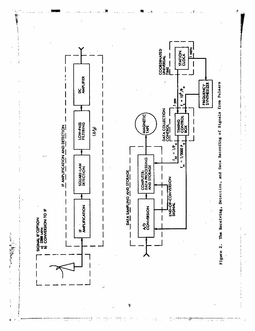
2. The Receiving, Detection, and Data Recording of
Signals from Pulsars 9
3. The 1-Second Pulses from the Station Clock_ at
DSS-13 and DSS-14, Goldstone, and Their Relation
to UT (station) 12
4. The Timing Control Box for Pulsar Data
Collection 14
5. Three Triangular Functions Overlying a Data Array .... 26
6. The templates of PSR 0031-07: (a) P = 0.943 sec;
(b) Expanded time scale 32
7. The template of PSR 0329+54: (a) P = 0.715 sec;
(b) Expanded time scale 32
8. The template of PSR 0355+54: (a) P = 0.156 sec;
The pulse has been smoothed by a window 160 _sec
wide. (b) Expanded time scale 33
9. The template of PSR 0525+21: (a) P = 3.745 sec;
The pulse has been smoothed by a window 2.2 ms wide.
(b) Expanded time scale 33
10. The template of PSR 0628-28: (a) P = 1.244 sec;
(b) Expanded time scale 34
vi
1980024809-005

F._ure5
Ii. The template of PSR 0736-40: (a) P = 0.374 sec
(b) Expanded time scale 34
12. The template of PSR 0823+26: (a) P = O.531 sec
(b) Expanded time scale 35
13. Tile template of PSR 0833-45: (a) 1' = 0.089 sec(b) Expanded time scale 35
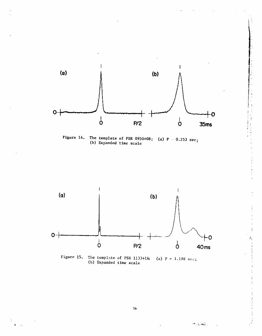
14. Tile template of PSR 0950408: (a) P = 0.253 sec
(b) Expanded time scale 36
15. Tile template of PSR 1133+16: (a) P = 1.188 sec
(b) Expanded time scale 36
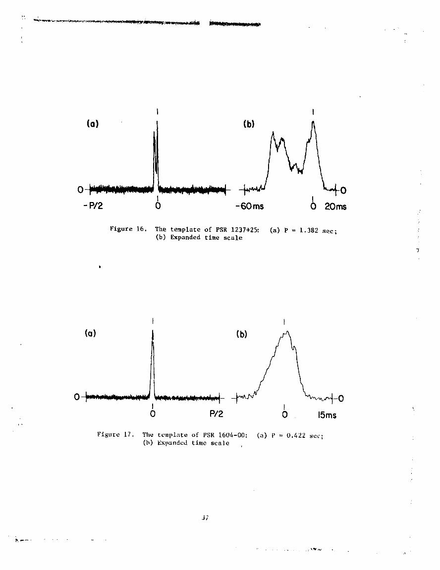
16. The template of PSR 1237+25: (a) P = 1.382 sec
(b) Expanded time scale 37
17. The template of PSR 1604-OO: (a) P = 0.422 sec
(b) Expanded time scaJe 37
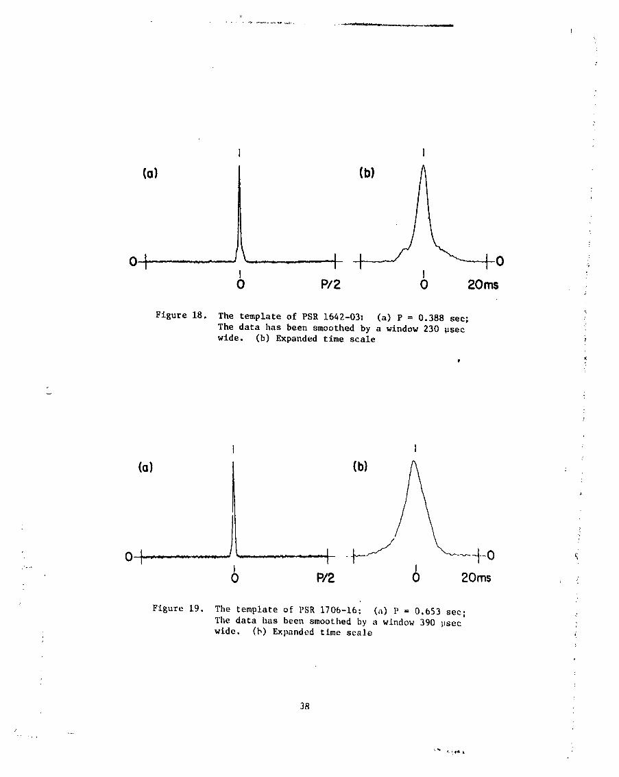
18. Tile templates of PSR 1642-O3: (a) P = 0.388 sec;
Tlle data has been smoothed by a window 230 _se_
wide. (b) Expanded time scale 38
19. The template of I'SR 1706-16: (a) P = 0.653 sec;
The data has been smoothed by a window 390 lJsec
wide. (b) Expanded time scale 38
20. The template of PSR 1749-28: (a) P = 0.563 see;
(b) Expanded time scale 39
21. The template of PSR 1818-04: (a) P = 0.598 see;
(b) Expanded time scale 39
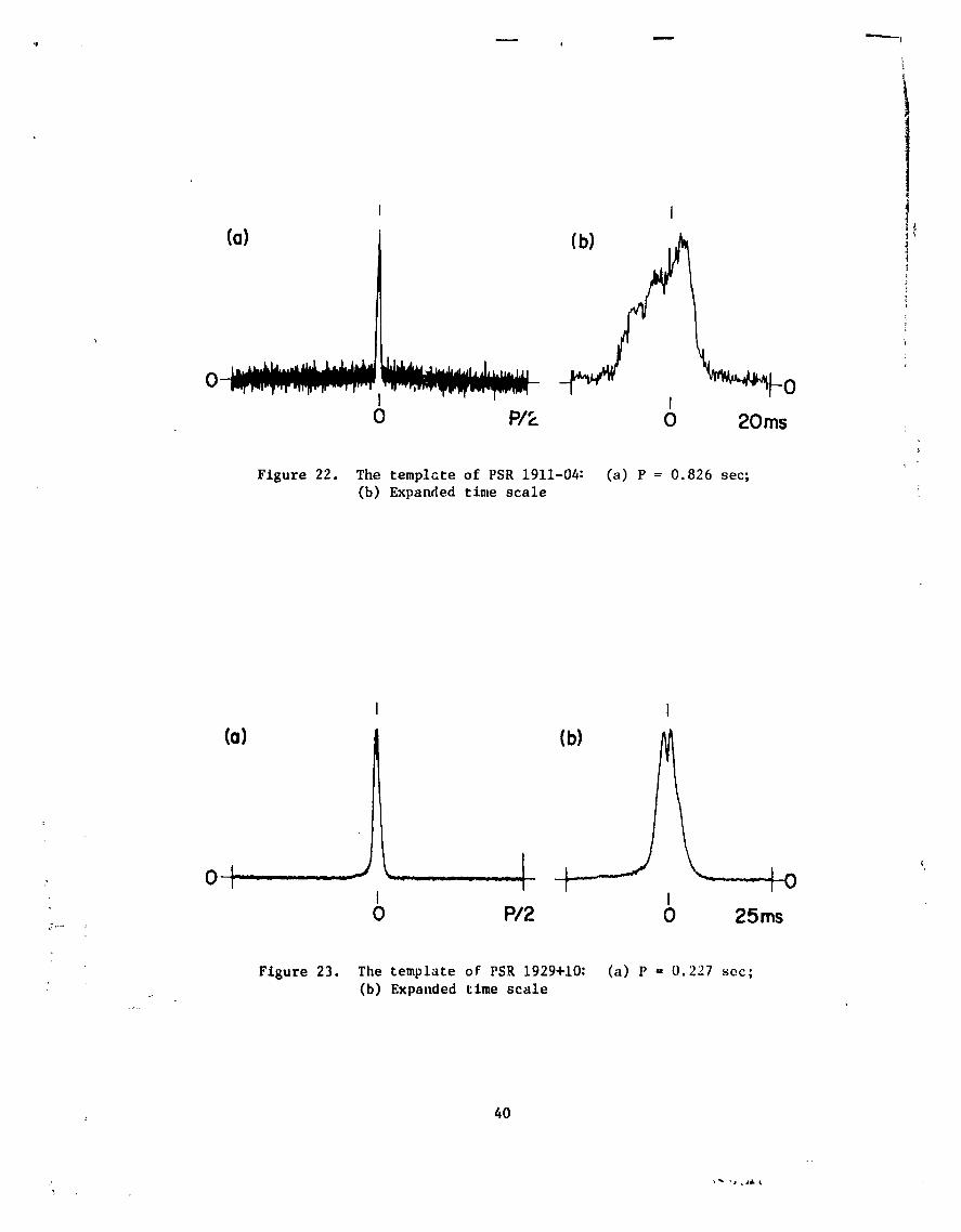
22. The template of PSR 1911-04: (a) P = 0.826 sec;
(b) Expanded time scale --- 40
23. The template of PSR 1929+10: (a) P _ 0.227 sec;
(b) Expanded time scale 40
24. The template of PSR 1933+16: (a) P = 0.359 sec;
- (b) Fxpanded time scale 41
f
25. The template of PSR 2016+28: (a) P = {).559 sec;
(b) Expanded time scale 41
26. The template of PSR 2021+51: (a) P = 0.529 sec;
(b) Expanded time scale 42
vii
1980024809-006
Ft_tffes
27. The template ,)f I'SR 2045-16: (a) P = 1.962 scc;'rile data has been smoothed by a window 1.2 ms
wide, (b) Expanded time scale - 42
28. The template of PSR 2111+46: (a) t' = l.Ol5 :;ec;(b) Expandt,d time scale, with the data smoothed
for display by .i window 2.0 ms wide 43
29. The template of PSR 2217+47: (a) t' = 0.538 sec;
(b) Exp,mded time scale, with the data smoothed
for display by ,l window 1 m.'; wide 41
_0. Shifting and Transforming the "l','mplate 49
I1. Computing the Cross Co,'relat ion Coefficients ......... 51
;2. An Example of tilt, Cross Corrcl:ltion Proces.s; PSI,'1818-04 on 27 Jan. 1979 at 16h 98 m OOs UT 32
!3. Correl,ltion Coefficients Versus Time l)etav Near
tilt, Pe,lk Shown in Figure ";). 55
]4. (;eometrv for C,llculating tile Phase Drift 59
35. Nomunclaturt, for Enumerating Pulses 60
36. An Ex,lmple of Drift in the Phase of I'SR 0833-43on 1 Dec. 1968 ,It 11 h 00 m O0 s (UT) O_
37. 'rime-of-Arriv,ll Residuals of bleasurements blade at
DSS-1 I and DSS-14 oil tile [qod if led Julian I)ate
(bl,lD) of Observation for I'SR 08_1-45 72
Tables
1. 24 l'uis,lrs Monitored at ,IPL ;It Frequencies of2295 blllz and 2388 HIIz 3
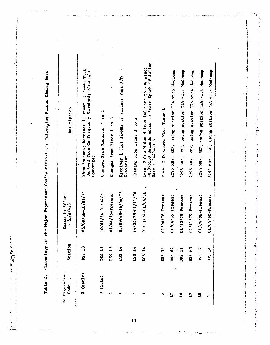
2. Chronology of the blajor Experimt'nt Configur,ttionsfor Collecting I'ulsar Timing Dat,t It)
_. The Configur,ltitul {',,des Corre,_pt_tldJng to Non-St_,ndard
Observing Frequent ies ................................. 11
4. Pulse Sme,lring lhle to l)isperslon ,lnd l'ost-I)¢t.ection
Fil ter ing I t)
5. (;eocentric Antenna Coordinates 64
6. Relations Used in Comlmt trig the GIlA of anObservil_g Stat ion 64
viii
1980024809-007

Tables
7. Elements of tile Precession M_itrix 66
8. PSR 0823+26: Geocentric Time._-of-Arrival 74
1980024809-008
SECTION I
INTRODUCTION
Natural sources of pulsating radiation were first observed in 1967
(Refs. 1, 2) by radio astronomers at Cambridge University in England.
These pulsating radio sources (pulsars) are exciting because they (1)
are thought to represent a stage in stellar evolution known as neutron
stars (Ref. 3), providing a probe of an extremely dense state of matter;
(2) exhibit changing, often dramatically so, behavior in the pulse per-
iod, signifying changes in the spin rate of the neutron star driving
the pulse generating mechanism; and (3) have large space velocities,
implying violent origins.
A series of measurements is being established using the NASA--
JPL Deep Space Network (DSN) which will allow a probing of tile neutron
star interior and a direct measurement of changes in spin r;_te and
angular motion. The purpose of the measurements is to measure the phase
of the pulse train at known epochs. It requires little imagination to
realize that the simultaneous comparison of the phase of a pulse train
at two different DSN stations represents either a measurement of the
difference between the station clocks, or a measurement of the location
of one station relative to the other. In navigation, one assumes the
clocks are synchronized. Differences in pulse phase are then attributed
to differences in location. We need only to replace one DSN station
with a spacecraft to complete the Illustration.
The purpose of this report is to describe in appropriate detail
the tm,hniques timed currently in the DSN for measuring the arrival time
I
1980024809-009
of a particular pt,l_e (alternatively, the phase of the pulse train
relative to a given epoch). Phase measurements were begun in September
1968 and continue to the present. The 24 pulsars included in this series
are listed in Table i with appropriate dates on _,.ich measurements began.
_n example of the results of this long series of measurements is presented
in Table 7.
Marly characteristics of the pulsars have been or can be deduced
from the measurement of pulse phase at a series of epochs if the epochs
occur often enough (weekly to monthly _,and eve[ a sufficient time span
(years). Usually a parameterized model of the pulsar is constructed
which is used to predict tne time-of-arrival of a given pulse (or the
phase of tile pulse train at a given epoch). The parameters are then
adjusted to minimize the mean square difference between the predictions
and the meas oments. The final wllues of the model parameters are
dependent on the planetary ephemeris used in the data renu,'timl, since
all observations are usually referred to the barycenter of the solar
system. The importance of this is clear when one realizes that 2 milli-
seconds flight time in the displacement of the barycenter amounts to as
much as 1 arc-secmld displacement in the position of the pulsar. E_rors
in the knowledge of the harycenter with time scales of tens of yoars
are caused by inaccur,,cies in the w_lues of the masses of the t,uter
planets. These slow curvil inear errors affect the wilues ,_f the higher-
order derivatives of the pulse period, ltence, though all current
, ephemerides may prt_ducv similar puls:ll model param_ toys, improved
ephenwridcs dvai iat_le twenty vcars fr_m_ m,w will produce significantly
different results. Tables of geocentric arriwll times, being important
2
] 980024809-0] 0

Table t. 24 Pulsars Monitored at JPL at Frequenciesof 2295 blHzand 2388 MHz
Entry Pulsar Start Date
I 0031-07 5 Mar 1970
2 0329+54 5 Sep 1968
3 0355+54 5 May 1973
4 0525+21 I Jun 1969
5 0628-28 30 Dec 1969
6 0736-40 I Oct 1970
7 0823+26 12 Feb 1969
8 0833-45 22 Nov 1968
9 0950+08 5 Sep 1968
I0 1133+16 25 Oct 1968
Ii 1237+25 I0 Aug 1969
12 1604-00 1 Oct 1970
13 1642-03 12 Ju] 1969
14 1706-16 I Oct 1970
15 1749-28 2 May 1969
16 1818-04 29 Dec 1969
17 1911-04 5 Mar 1970
),
18 1929+10 29 dun 1969 '
19 1933+16 23 Dec 1968
,'() 2016428 5 Sep 1968
?) 20214-51 30 Dec" 1969
.'.' 2045-16 ]0 Dec 1968
.!_ '?111+!_, 30 Dec 1969
24 2217+./)) 30 Dec 1969
3
1980024809-011

archiw,_ of pulsar t>ehavi<_r, _lre indepe,ldenL of sm:l]l c'h:ln,;u,: _1 LI_.
ephemerides of Lhe pl;uneL_. They form the exported fc_rm of tht: _bsur-
vaL ional results.
The measurements were performed earlier at a frequency of 2388 MHz
on the 26-m antenna at Deep Space Station 13 (DSS 13) and the 64-m
antenna at DSS 14. Current observations are at 2295 MHz, utilizing all
facilities at Goldstone and in Spain. Detected pulsar signals are
sampled, integrated and recorded on magnetic tape. Data collection and
recording is discussed in Section II. The data are then edited and, for
the early years, collated according to the pulsar, as described in Sec-
tion III. The collated data, stored on magnetic tapes, was used to
derive a template for each pulsar, representing the average power level
across a pulse t_f radiation. The template is then cross correlated with
each data record of the particular pulsar to obtain an estimate of the
pulse arrivat time. The procedures used in constructing the templaLes
is described in Section IV and the cross correlation process is dis-
cussed in Section V. The correction of the arrival time cotimates for
various small effects is discussed in Section VI. A sample list of
geocentric times-of-arrival is presented in Section'VII.
4
1980024809-012

SECTION Il
DATA COLLECTION
A. RECEIVING, DETECTION, AND RECORDING
It was shown shortly after the discovery of pulsars that they could i
be detected at 2295 MHz (Ref. 4). Shortly thereafter, in August 1968,
JPL observations at 2388 MHz were b- ;unusing the 26-m antenna of DSS 13
at the Goldstone complex. 't_e_Ide bandwldths (about 12 MHz) and the 't
_, _ low system temperatures (about 16 K) aJlowed detection of three of the , _
first four pulsars discovered Over the following months the observa- ;
: _ tlons have been expanded to include 24 objects, utilizing all antennas ?
_ at Goldstone and Madrid. ?
: il T._ereceiver consists of the antenna, a right circularly polarized
! feed horn (left circularly polarized at 2388 MHz), a;_da maser pre- _
amplifier followed by conversion to and amplification at intermediate
; frequencl_, (IF). Low-loss cabling then carries the signal to the
i receiver room for more IF amplification. The receiver bandwidth is \
limited to 12 MHz by either the IF portion of the receiver or by a _g e
i "filter inserted for that purpose. Square-law detection of the signal }
_, is then performed, followed by low-pass filtering. The_ovtput of the
low-pass filter is amplified by a wldeband DC amplifler to a I- to °
i 2-volt level. Subsequently, the signal is converted to digital form _i_
_' ! in a sampling process. The integration time (see Ref. 5 for a deflnl- .
_; } tlon) of the post-detectlon fllter is chosen to match the time Interval }
g i between analog-to-digltal (A/D) conversions. '
{ _,e data processing, from sampling to the dumping onto magnetic ,
tape, is u-_cr computer control. The detected signal is sampled at a
5
a?
1980024809-013
rate equal to 5000 times the apparent pulse period, _:orresponding to
sample intervals of 50 _sec up to _00 _sec. Converted to a digital sig-
nal by an A/D converter, the samples are stored in the memory of an
SDS 930 computer or a standard station Modcomp computer. Data samples
are superimposed modulo the pulse period. Samples from 500 pulse periods
are superimposed congruently. Then a 5000-word _rray re_resenting the
superposition of 500 pulses is dtunped onto tape. This accumulation of
pulses continues until (a) detection is ensured, or(b} it is clear _the _
: pulses are too weak at this time to be observed. Accumulations rarel-y.l
run more than one hour.
The form of the recorded data is sketched in Figure 1. The pulse
is sitting on top of a system noise power corresponding to a temperature Ii
The peak equivalent temperature of the pulse is Tp. The 5000 i_Ts•!
samples spanning one pulse period are ulotted from left to right. Thei
time of the first data sample, plotted at the left, corresponds to a ,i
particular epoch of Universal Time _UT) as recorded _ the station. I
This start time is recorded in UT (station). The train of received
pulses then has a particular phase relative to the start time. The
pulse train is folded in upon itself to beat down the effects of receiver !
noise fluctuations. Rather _han think in terms of the phase of the
< pulse train, we ask for _he arrival time of the first pulse after the
%s_art time. Hence, the pulse delay is added to the UT (station)epoch
Lf
_' corresponding co the start time to yield _n epoch for the arrival time
_: of the pulse.
The phase of the pulse train may not remain constant during the
supr -positlon of many pulses. The subsequent drift in phase requires
that a correction be applied to the measured pulse delay. This
%
6
1980024809-014

, 7
1980024809-015
, correction is discussed in Section V[, D. Small corrections are required i _"
_ in the start time and in tlleUT (station) defined by a particular clock, i )These corrections are discusspd in this section and in Section VI.
B. THE S'..,tEM,IONFIrdRATION CODES _
The measurement system is shown diagrammatically in Figure 2. The
experimental hardware is grouped into units defined by the dashed boxes, i _
%
Each subsystem so defined has been interchanged with other similar sub-
systems, causing significant changes in the measured phases. Hence, a i :"
" system configuration code has been constructed to alert the analyst to - ¢
" changes in the system. The code varies from 0 to 21, representing 22
' significantly distinct combinations of antenna, receiver, observing 4
frequency, computer, data collection controller, and station clock. A ;_
summary of the basic- configurations (0-5) and (17-21) appears in :_
,/
Table _ Additional configuration codes (6-16) were created to denote
the use of an observing frequency of 2295 MHz or 2328 Mllz, and their :
relationship to the basic codes are shown in Table 3. Left circular i ,! /
polarization (LCP) is to be assumed unless specified as right circular
polarization (RCP).
Since the system configurations do not change in principle 'i :
from one to the other, only configuration 0 is described in detail.
_, Highlights of the other configurations are noted in the following para- _ _'
graphs. Configuration 0 Includes the 26-m antenna at DSS 13. The radio _{ _.
: frequency bandpass is determined by the IF amplifiers. The final IF _ ,
:" amplification, detection, and low-pass filtering is done by a receiver _ =
(labeled as receiver i) built in 1968 by C. F. Foster. The timing con- } _"
trol box was designed by G. A. Morr_ and is labeled timer 1. i _'
"" 8
• _2
............. S
1980024809-016
1980024809-017
1980024809-018

_p_ _ :_ ....: __r'_ "__-'__<_'_'___
i\
Table 3. The Configuration Codes Corresponding ,.to Non-Standard Observing Frequencies
ObservingConflguraclon, Configuration Frequency (_z) Description :,
8 } 0 2328 _9 2295
10 } 1, 2, 3 2328 _:Ii 2295e
87 } 4 22952328 - _i
6 5 2295Denotes a correction w,s made to
• 12 Any standard post-detectlon Af_ _r
13 4 2295 RCP
14 5 2295 RCP
15 5 2295 DSS 13 via link toDSS 14 ::
16 5 2295 DSS 12 via link to
DSS 14 _
The relationship between the epoch-defining 1-second pulse and ,..
Universal Time as disseminated at the station, UT (station), is shown
; in Figure 3 along with the relationships for the other codes. Exact
_ relations between UT (station) and Coordinated Universal Time (UTC) is i_ :
#_i_- discussed in Section VI. Data sampling in configuration codes less -_
_i_1 than 17 is performed by a 12-bit A/D converter with a 40 _sec con- ;_ I version time. The samples are stored in an SDS 930 computer having a
16,384-word memory. The station telemetry processor assembly (TPA) :
is used in codes 17 or larger.
_ ,
t
1980024809-019

1980024809-020

The final IF amplification and detection is performed in the steps
shown in Figure 2. The first unit buiit was transported between DSS 13
and DSS 14 unttI 10 Jan. 1974, when it was permanently installed at
DSS 14. This unit was replaced at DSS 13 by a programmable unit butit
by C. F. Foster (described in Ref. 6 and labeled receiver 2). This' ?
change is not noted by a configuration code change. Hence, code 0 con-
sists of an early phase (pre-lO Jan. 1974, Julian date 2442057.5) and
: a late phase (post-lO Jan. 1974). s
The timing control box used here is not described elsewhere, so= #
a block diagram is presented here for tutorial purposes. Other control #
boxes used in other configurations operate on the same principle, but,
differ in complexity and detail. Careful study of Figure 4 shows that
a string of fast and slow pJlses are generated by the timing control
box to control the data sampling. The pulses are derived by counting ?
i
down pulses from a frequency synthesizer, starting at a well-defined
time by gating the synthesizer output. The gate must be armed and then
a 1-see pulse must be received before counting begins. To assist the
operator in determining on which second the counting started, the 1-sec
pulses are counted down by 10 so that counting wiI1 start modulo 10
seconds. •
; The fast pulses, occurring every P /5000 seconds, where P is the ha a
apparent pulse period, are used to strobe the A/D converter. The slower
_ pul_c_, occurring every P seconds, are used to control the data transfer
into core memory. On the first slow pulse, a computer interrupt is
coincident with the slow pulse commands the A/D converter to begin
operation. About 20 t_sec later the end-of-convertlon (EOC) interrupt _
force_ the computer to accept the new word, and about 20 _sec after ,;
,\
-?
1980024809-021

1980024809-022

, interruption, the word has been added to the proper memory location.
[ Note that although it takes time to set up the Computer to accept data,
; i}[
the EOC pulse arrives after the setup, so the first sample accepted is, ;
< Jn fact, coincident in time with the l-sec pulse modulo one pulse period. +t
However, a configuration exists in which the first sample is not coinci- ,:
dent, and a correction must be applied. ,_
The data sampllng and superpositlon is under the control of az
program written by G. A; Morris. The program also controlled the writ-
ing of the results onto magnetic tape for further reduction.
The apparent p_riod P is the result of the I_pplez effect causeda _
?
by Earth's motion about the barycenter of the solar system. Tables of
P are computed using a barycentric ephemeris of Earth and a crude buta
+ adequate model of the pulsar. The model includes the ceIestial
coordinates of the object as well as the barycentrtc model of the pulse ,+
period (usually a period P0 at some epoch to, and the first derivative _
"i The values of P are tabulated at 15-mlnute intervals between rise
i and set for any given day. The operator then chooses the value cor- }+
responding to the middle of the intended interval of pulse integration. -_
Configuration i consists o_ the 64-m antenna at DS$ 14, the same
IF amplification and detection unit, and the same timing bpx.used in }
the early configuration O. A 12-MHz IF _ilter is added to the chain to )
:; limit the IF bandwidth. The computer is again the SDS 930_ The A/_ :)
_ - _ converter, howeveri responds within 5 _sec of being strobed wlth a
_ _ convert command. _k_computer, requiring about 20 _sec to arm the +
•+ _ interrupt and start the data flow, misses the first data sample. The
• _
i data stream is then shifted Pa/5000 seconds later in time. Thls shift +: +
Is as large as 0.8 msec and is added to the UT (station) recorded by
J +the operator. + '_
l 7
1980024809-023

i
i_ Timer i was designed to accept the rising edge of a positive l-sec
pulse as the definition of UT (station). The l-set pulse distributed
at DSS 14 is negative-going, the rising edge being coincident with UT!
(station). The necessary pulse inversion then causes the timing box
to begin counting earlier than intended by a time equal to the width of •
the l-set pulse. This amounts to i00 _sec in configuration 1 and
200 _sec in configurations 3 and 5.
A programmable timing box, designed, built, and programmed by
A. G. Slekys (Ref. 7) replaced _he original timing box at DSS 14. This
timer is labeled timer 2, and pertains to codes 2 and 3. A failure
occurred in timer 2 which caused the start times of code 3 recorded
between Julian dates 2442460.5 and 2443105.5 (17 Feb. 1975 and
y
23 Nov. 1976) to be earlier than intended. The correction is a sub-
traction of nearly I second. The exact correction was determined from
a preliminary fit of a model of the pulsar emission times to the data.
A correction of -0.996550 Seconds to the start time aligned the affeLted
arrival times with the times measured at DSS 13 (code 0 and 4) and with
those unaffected from'DSS 14.
Timer 1 was replaced at DSS 13 on I April 1975 by a programmable
data collector/tlmer designed by S. S. Brokl (Ref. 8) and programmed by
K. I. Noyd. This timer is iabeled timer 3, and pertains to conflgura- i
_ tion code 4.
_ Occasionally a non-standard value is used for Af_ in the post-
detection filtering. If a correction is applied, the configuration code
is 12, corresponding to a correction to code 0 for dates prior to 1970
and to code 5 after 1976. (None occur in the intervening years.)
1980024809-024

r
f,
During the first half of 1979, the SDS 930 computer was phased out
of service and removed in June 1979. This created thg need to transmit
IF signals over the microwave comuntcation links to DSS 14 for data
recor21ng. The required 12 MHz bandwidth was obtained from the 6 MHz ,_
bandwidth of the link by folding the IF spectrum about the midpoint _
during base-bandlng. This technique was also used in obtaining signals
_ from DSS 12. The configuration codes 15 and 16, then, indicate the = _i 4-
recording at DSS 14 of signals from DSS 13 _d_DSS_I2 ,,resp_ti_eiy_ i:_i_'i'(°i:il;/_:--_:
the use of the telemetry processor assembly (TP_)found in:_ll:D_:: ......-_=-'"=7,_:_}_[_o-5_'_-_JL_;:;_,_
stations except DSS 13. The scheme was constructed, by J2 and M. Urech"S_' _7(!_<2:2.= ,_'Li;:;:i_-
at DSS 62. Many of the hardware functions of Figure 2-are-duplicate_i -........'-_:_2_::__:'':_"_;W,_t_:'_'_
i by their software. The data output is still in the form of 5000-word _w:_= ' ._-:e_
records on magnetic tape. The configuration cod- _.°fthis-scheme for _,.:_;,_• ,- ,/{.J
? each station is listed in Table 2. ,% , j;.
C. EFFECTS OF RECEIVER PARAMETERS ON :THE ARRIVAL TIN ...... - - q
Pulsar slgnals are dispersive since the interstellar plasma :Intrb- I, ,_i-
duces a frequency-dependent group velocity. A broadband pulsem. CoV_ing _. _ r:'_
the radio spectrum from 30 HHz to i0 GHz, will arrive at the rece_vlng ' : _!-
antenna and sweep through the receiver paasband at a ra_e given by
S KF3/DM (MHz/sec) (I) "' _ lib
At _
:_ where the bandwidth B is in MH_, the observin_ frequency T Is In MH_. _5r,_
, _t is in seconds, DN is the dispersion measure in parsecs (pc) c_ "3, -_
and K = 1.205043 x i0"4. Let Eq. (i) define the amount of smear /_t in _ .,_
,I the received pulse shape when all the other parameters are known. At '_I ;
F = 2388 Mllz, a dispersion measure of I0 pc cm causes th,_. pulse to4
, _
1980024809-025
smear 75 psec when the receiver passband is 12-MHz wide. The smear is
750 _sec when the dispersion measure is I00.
Computed values of smear are presented in Table 4. As long as the
bandpass parameters remain fixed over the years, the dispersive effect0
should not affect the measured arrival times. However, changes in a
filter element or the slight alteration in the tuning of the maser
_ amplifier will change the frequency centroid of the passband. This, in
turn, will change the time centroid of the detected pulse. The mag-
nitude of this effect must be determined experimentally and has not
i been done. The effect is expected to be small since it is not the
i limits of the passband that change, but on]y the shape
i The response of the post-detection filter is chosen such that the ]ii integration time z is close to the time interval Pa/5000. In the case
of these simple RC filters, _ = 2RC (Ref. 5), where R and C are the
filter resistance and capacitance, respectively. Considerable care is I;i i _
I exercised in using the appropriate filter combination for each pulsar I_
throughout the observations. Use of non-standard values of T could cause
up to 200 usec of time shift in the arrival time. The values are listed
: in Table 4. Note that the change from pre-lO Jan. 1974 (Code O) to !I
post-lO Jan. 1974 (Code O) is principally a change in the post-detection !
filters, and much care was taken to duplicate the previous values of _ ,_
_ in the new filters.
_. A quantitative measure of the system perform.nee is given by the
_a _ ratio of o, the root-mean-square (rms) value of the noise fluctuations
about the mean, divided by _, the mean. Letting N represent the : _
;number of pulses superimposed,
C
} _Lg
184
I
1980024809-026
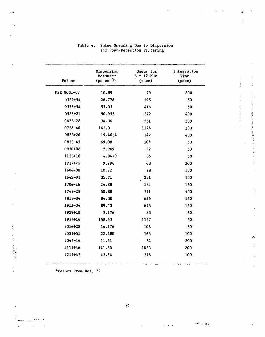
Table 4. Pulse Smearing Due to Dispersion
and Post-Detectlon Fi]terlng
Dispersion Smear for IntegrationMeasure* B ffi12 HHz Time
Pulsar (pc cm-3) (_sec) (_sec)
PSR 0031-07 10.89 79 200
0329+54 26.776 195 50
0355+54 57.03 416 50 _0525+21 50. 955 372 400 4.
0628-28 34.36 251 200
0736-40 161.0 1174 100
0823+26 19.4634 142 400 _:
0833-45 69.08 504 50 •
0950+08 2.969 22 50
1133+16 4.8479 35 50
1237+25 9.296 68 200
1604-00 I0.72 78 i00
1642-03 35.71 261 i00J
1706-16 24.88 182 150
1749-28 50.88 371 400
1818-04 84.38 616 150
1911-04 89.43 653 150
1929+10 3.176 23 50
1933+16 158.53 1157 50
2016+28 14.176 103 50
2021+51 22.580 165 I00%
: 2045-16 11.51 84 200
_ 2111+46 141.50 1033 200
!:_ 2217+47 43.54 3]8 i00,!
*Values From Ref. 22
19
1980024809-027

I
One expects for N = 500, _ = 50 _sec and B = 12 _Iz, Lhat o/_ _ 0.OUiS.
Throughout the years of data collection this parameter has varied between
0.0013 and 0.0025, corresponding to 42 psec < T < 59 _sec. Hence, the
values of integration time listed in Table 2 were stable to within
16 percent of the tabulated value.
2O
1980024809-028

SECTION III
EDITING AND COLLATING
A. EDITING THE DATA
Successfully measuring the time-of-arrival of a pulse near a
given epoch does not ensure that the result is free of biases. The
editing process involves detecting the biases, correcting tilemeasure-
ment if the reason for the bias is known, or omitting the measurement
if the reason for the bias is known but does not allow correction. A
good example of a correctable situation is the use of a receiver fre-
quency other than the 2388 MHz frequency used in most of the measurements.
A preliminary model (positiop and pulse period) is devised for
each pulsar. These models are used in a computer program of adequate
accuracy to predict pulse arrival times at the barycenter of the solar
system. A barycentric ephemeris of the Earth is used to refer tlle
measured arrival times to the barycenter and a residual (measured minus
predicted) arrival time is computed. The occurrence of a residual that
is large compared to the average fluctuation is cause for further
investigation.
Several properties of the pulsar or the system are directly
responsible for the need to correct or omit the arrival time Measure-
ment. They are :
(1) Scintillations
Interstellar clouds of ionized hydrogen impose varlat.ions
on the received pulse power. The t_nle scale uf the fluc-
tuations is on the order of tens of minutes. If the pulsar
is far enough away, and several are, large fluctuations in
the pulse power force tho signal tlo_ into tile receiver
1980024809-029

noise for many minutes, causing a simrious estimaLe of thL
pulse arrival time,
(2) Start Times
The early timing box divides the incoming l-see pulse by
I0 (see Fig. 4), allowing the counting to be started at
well-deflned lO-sec intervals. It is imperative that the
counter status register be synchronized with the station
clock, modulo I0 seconds; i.e., on the even lO-second mark,
the counter should read O. Occasionally synchronization is
lost. In these cases it is easy to deduce how many integral
seconds (never more than i0) the start time has to be
retarded or advanced to obtain the true start time.
(3) Receiver Frequency
Dispersion caused by the interstellar plasma causes the
arrival time to be a function of observing frequency. Using
a non-standard receiver frequency produces a _orrectable
error (see Section VI, F).
(4) Post-Detection Filter
Occasionally a non-standard filter width was used, resulting
in unusual time delay through the filter. A correction is
readily applied.
During the summer months of 1969 a bad detector connection
caused unusually large (~I ms) time delays. The corrections
for this effect were derived by computing the autocorrelation
function of the system noise, the width of which then gave
the effective time constant of the filter. Both situations
are labeled as system code 12 (see Section II, A).
22
1980024809-030

f(5) Miscellaneous
In a very few cases the reasons for a large residual are
unknown. Common experimental situations in such cases
are receiver tuning problems, repeated power failures, and
radio frequency interference (RFI). The measurement results
are usually omitted.
B. COLLATING THE DATA
A data tape produced at Goldstone contains data files corre-
sponding to the pulsars observed during a particular observing session.
This format is inconvenient for producing average pulse profiles. (These
profiles, discussed in Section IV, are a necessary part of optimally
estimating the pulse arrival time). Therefore, the early data files of
a particular pulsar were gathered onto one or more magnetic tapes in the
order they were collected at Coldstone. Preliminary editing took place •
5
during this process, to delete obviously faulty data. The main cause
for omission at this stage is RFI. These data were used to compute
the mean pulse profile presented in Section IV.
Data collected after August of 1972 is not collated according to
pulsar. Data files are merely written onto magnetic tapes in the order
they were collected without regard to the particular pulsar. The files
were condensed by editing the data and filling each tEpe completely.
Estimates of arrival times are obtained after each tape is filled (every
2 to 3 months).
"_ 23
1980024809-031

SECTION IV
PULSE-SHAPE TEMPLATES
In the presence of white noise the maximum signal-to-noise (S/N)
ratio for the output of a particular filter can be obtained when th_
filter response has the same form as the input signal (a matched filter).
The required matched filter is realized by cross correlating a received
pulse with an estimate of the nolse-free shape of the pulse. The esti-
mates of the noise-free pulse shapes are obtained by superimposing many
thousands of pulses to average down the effects of noise. The result
is referred to herein as a template.
The proper registration or alignment of the pulses needs to be
obtained to build a template with a minimum of smearing. Two passes,
each described below, are used to optimize tH4 registration. Correlation
with a triangular function is first performed to obtain first-order
estimates of pulse position within the data records. The template posi-
tion in the data array corresponding to the maximum cross correlation
coefficient is defined to be the pulse position. The numbers in each
data record are then shifted circularly by the amount required for proper
registration with all the other data records. Adding all the records
produces a preliminary template. This template is cross-correlated with
the original data to provide new estimates of pulse positions within
the data arrays. The second result of the addition of all the properly
registered data is taken as the correct average pulse shape. F .ally,
the central 4096 words of the 5000 word array are used to form the tem-
plate. See Section V regarding the choice of the 4096 words.
24
1980024809-032
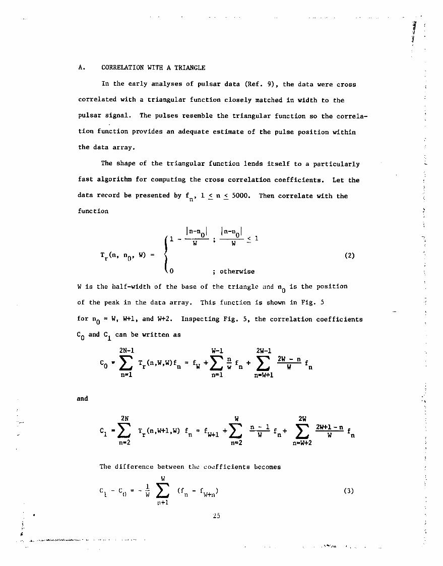
A. CORRELATION WITH A TRIANGLE
In the early analyses of pulsar data (Ref. 9), the data were cross
correlated with a triangular function closely matched in width to the
pulsar signal. The pulses resemble the triangular function so the correla-
tion function provides an adequate estimate of the pulse position _thln
the data array.
The shape of the triangular function lends itself to a particularly _i
fast algorithm for computing the cross correlation coefficients. Let the _"
data record be presented by fn' I _ n _ 5000. Then correlate with the _i
function
In-nolIn-n01
<i _
i - W ; W -
Tr(n, no, W) = (2) _"
0 ; otherwise !
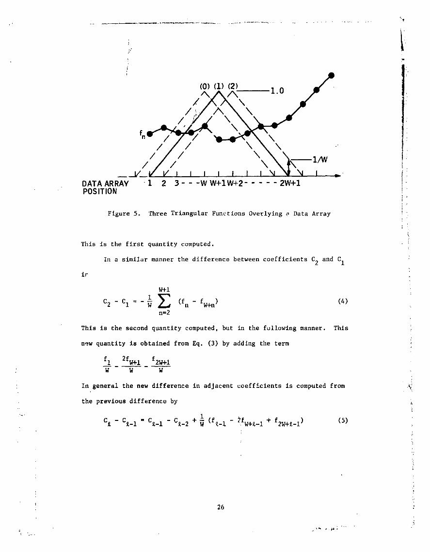
W is the half-width of the base of the triangle and nO is the position
of the peak in the data array. This function is shown in Fig. 5
for no = W, W+I, and W+2. Inspecting Fig. 5, the correlation coefficients
CO and Cl can be written as
2N-I W-I 2W-i
CO = Tr(n'W'W)fn = fw + w fn + W n
n=l n=l n=W+l
and ,_
2N W 2W
n=2 n=2 n=W+2
The difference between the coefficients becomes
W
ct - % -- - w (fn - fw+n) (3)n+l
' 25
1980024809-033
/
(0) (1) ('2) _-
DATA ARRAY - 1 2 .3,- - -W W+IW+2- 2W+lPOSITION
Figure 5. Three Triangular Functions Overlying a Data Array :
This is the first quantity computed (•
In a similar manner the difference between coefficients C2 and C1
W+I
C2 - C1 = - W (fn - fW+n ) (4) _n=2
This is the second quantity computed, but in the fullowing manner• This
new quantity is obtained from Eq. (3) by adding the term
fl 2fW+l f2W+l
W W W
In general the new difference in adjacent coefficients is computed from
the previous difference by
c_ - c__1 = c__1 - c__2 + _ (f_-i- _.fw+_-i+ _2w+_-i) (5)
26 ,'_
1980024809-034
The value of C_ relative to the coefficient CI is calculated by accumulat-
ing the sums C£ - Cg_ 1 + C£_ 1 - C__ 2 from Eq. (4) through the many steps
suggested by Eq. (5):
C3 - C2 + C2 - C1 = C3 - C1
C4 - C3 + C3 - CI = C4 - CI
C_ - C___1 + C___1 - C1 = C£ - C1
The position of the peak of the triangular function corresponding
to the largest value of C_ - C1 denotes the position of the pulse in the
data array•
B. CORRELATION WITH THE TRUE TEMPLATE
The cross correlation function C(_) of two continuous functions
is written as
!
c(T) = [p(t)e(t - T) dt (6)J
where p(t) is the pulse power as a function of time t, e(t) is the
expected pul_e shape (the pulse template) and I is the displacement in
time of the two functions relative to some well-defined reference time.
In the discrete case encountered here, the corr,,lation coefficients can
be evaluated by directly performing the operati_,n suggested in Eq. (6).
However, it is much faster to use Fourier analysls techniques. Direct
ewlluation of Eq. (6) requires 2.5 x 10⁷ multiplications, while using
the fast Fourler transform (FFT) algorithm requires only about i._ x 105
multiplications.
27
!,
1980024809-035
Consider the Fourier t_ansforms of the functions involved. The
transform of the correlation function c(_) becomes "
/ -I2_s_C(s) = p(t) e(t - _) dt e dT
where s Is the transform variable. Interchanging the order of integration, _
: C(s) = t) e u) e du dT _
c(s)= P(s)E(-s) (7)
where P(s) and E(s) are the transforms of p(t) and e(t), respectively.
Hence, the procedure is to calculate E(-s) for each template (calculated
only once), P(s) for the data record, and then the complex function C(s).
Inverse transformation of C(s) yields c(_).
The FFT algorithm is used in a form that takes advantage of the fact
that a Fourier transform of a real function is the sum of a real even=
function and an imaginary odd function. Hence, if the data array is L ,%
samples long, only L/2 values need be calculated in the transform. See
Ref. I0 for the original work on this form of the algorithm or the detailed
discussion of its use by Brigham (Ref. 11). Briefly, the data is placed
in an array L samples long, where L is a multiple of 2. Pretending that
!.
the array is complex of dimension L/2, an FFT is performed on the complex
_rray. A final step is needed to unscramble the result into (L/2) - I
: complex pairs, one 0-frequency value, and one Nyquist-rate value. Alter-
natively, putting complex data such as the quantities P(s)E(-s) in this
form, the Inverse of the above process can be formed. Software to per-
form the calculations was mrttten for this project by G. A. Morris. 2
28
1980024809-036
_ _ _--_I_ .... I ] ....... "I_l _] .............................. II I *ll IlII
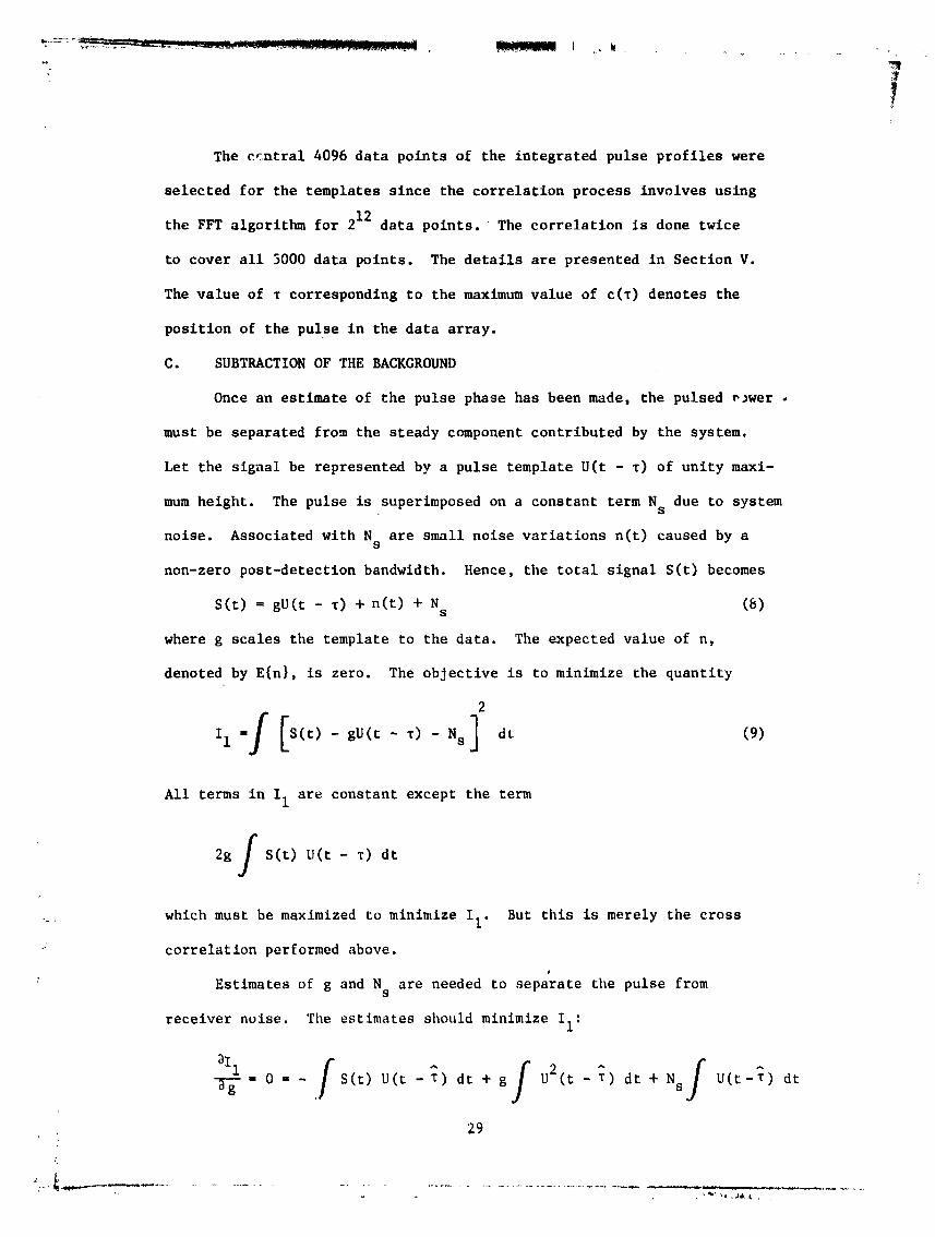
7The central 4096 data points of the integrated pulse profiles were
selected for the templates since the correlation process involves using
the FFT algorithm for 212 data points. The correlation is done twice
to cover all 3000 data points. The details are presented in Section V.
The value of T corresponding to the maximum value of c(T) denotes the
position of the pulse in the data array.
C. SUBTRACTION OF THE BACKGROUND
Once an estimate of the pulse phase has been made, the pulsed rower ,
must be separated from the steady component contributed by the system.
Let the signal be represented by a pulse template U(t - z) of unity maxi-
mum height. The pulse is superimposed on a constant term N due to systems
noise. Associated with N are small noise variations n(t) caused by as
non-zero post-detection bandwidth. Hence, the total signal S(t) becomes
S(t) = gU(t - T) + n(t) + N (8)s
where g scales the template to the data. The expected value of n,
denoted by E{n}, is zero. The objective is to minimize the quantity
2
Ii =f IS(t) - gU(t - _) - Ns] dt (9)
All terms in I1 are constant except the term
2gf S(t) U(t - _) dt
. which must be maximized to minimize II. But this is merely the cross
_: correlation performed above.
Estimates of g and N are needed to separate the pulse froms
receiver noise. The estimates should minimize Ii:
-_g i 0 = - S(t) U(t _) dt + g (t - _) dt + Ns U(t-_) dt
_9
1980024809-037
r,
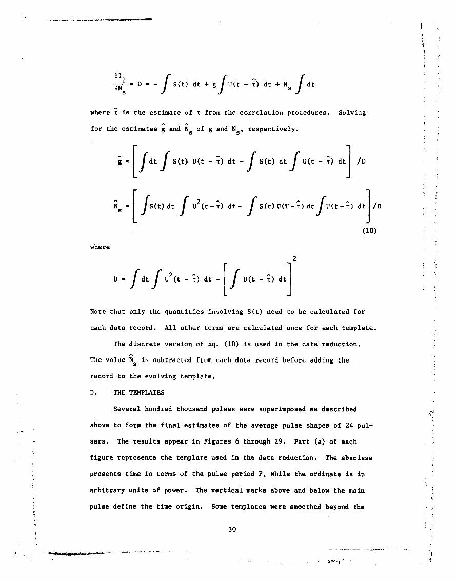
_--_-= 0 = - S(t) dt + g U(t - _) dt + N s dt ; :s
i
where _ is the estimate of T from the correlation procedures. Solving
for the estimates g and Ns of g and Ns, respectively.
= dt S(t) U(t- _) dt- S(t) dt U(t -_) dt /D
Ns = (t) dt U2(t-_) dr- S(t) U(T-_)dt (t-_) dt /D i :y
L
(io) :
where
2 _
Note that only the quantities involving S(t) need to be calculated for
each data record. All other terms are calculated once for each template.
The discrete version of Eq. (i0) is used in the data reduction.
The value Ns is subtracted from each data record before adding the
record to the evolving template.
D. THE TEMPLATES
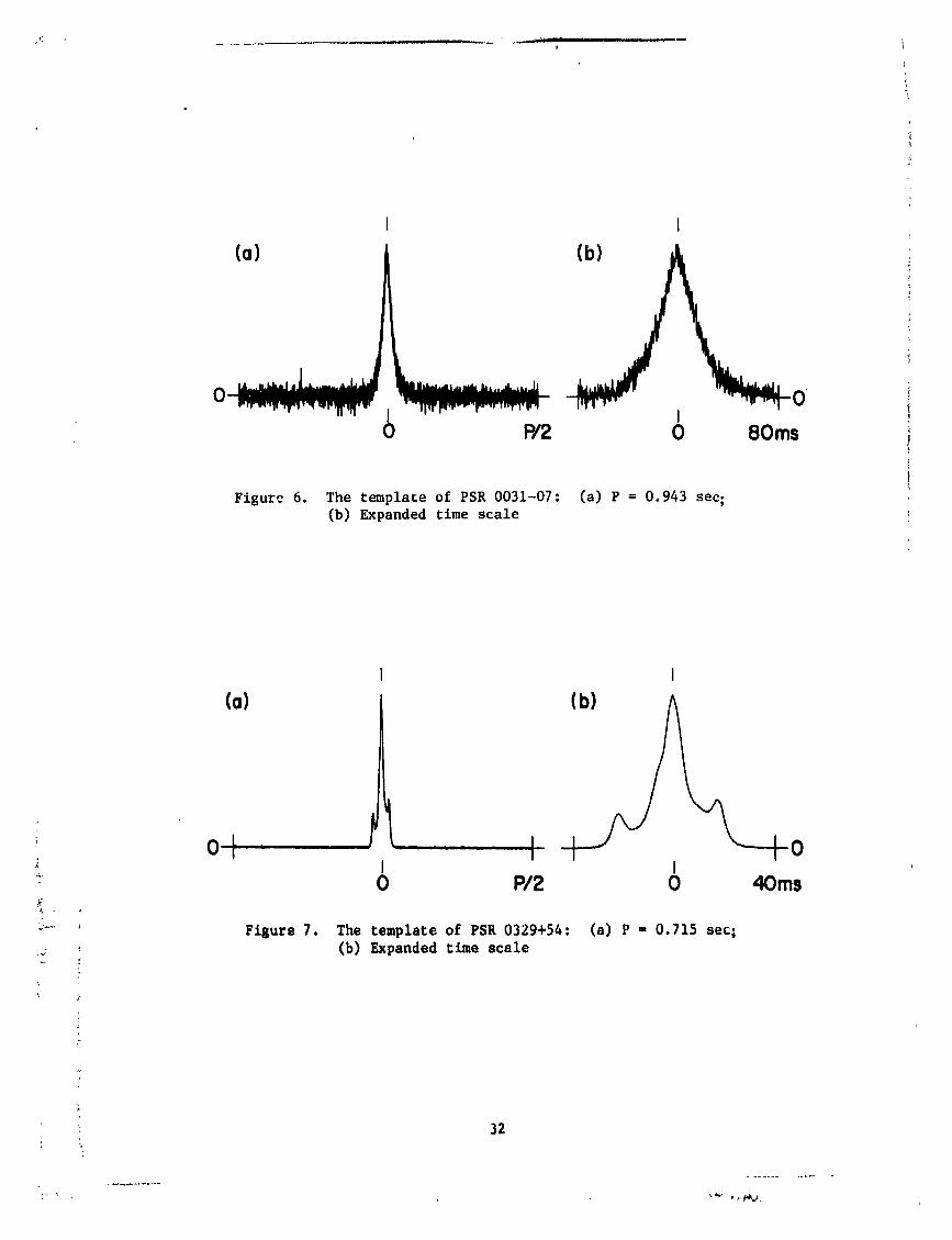
Several hundced thousand pulses were superimposed as described ,._
above to form the final estimates of the average pulse shapes of 24 pul-
sars. The results appear in Figures 6 through 29. Part (a) of each
figure represents the template used in the data reduction. The abscissa
presents time in terms of the pulse period P, while the ordinate is in
) arbitrary units of power. The vertical marks above and below the main :
_- pulse define the time origin. Some templates were smoothed beyond the s
_; ] I'
30 .}
¢
1980024809-038
amount inherent in the receiver. The smoothing was obtained by convolving
a sinc(c) function of the appropriate width _ith the original data. The
amount of smoothing noted in the figure caption represents the interval !
from the peak to the first zero of sine(t). A quantitative discussion
of the choice of smoothing is presented in the next section.
Part (b) of each figure presents the details of the pulse on an?
expanded time scale. If the data has been smoothed more than in part (a)
of the figure, the amount of smoothing is noted. The position of the T
pulse relative to the vertical marks above and below the main pulse
defines, for that pulsar, the "zero phase" condition relative to a given
epoch; i.e., to obtain a zero tlme-of-arrlval residual relative to a
given epoch, the vertical marks must be coincident with that epoch.
E. T_PLATE SMOOTHING
The accuracy with which one can estimate the arrival time of a pulse
increases as the rcndom fluctuations in the signal decrease and as the
sharpness of the pulse increases. However, attempts to smooth the signal
to lower the effects of receiver noise also tend to destroy the sharpness
of the pulse. A compromise must then be reached. This is done by esti-
mating the uncertainty in the arrival time measurement when the signal-to-
noise ratio is large.
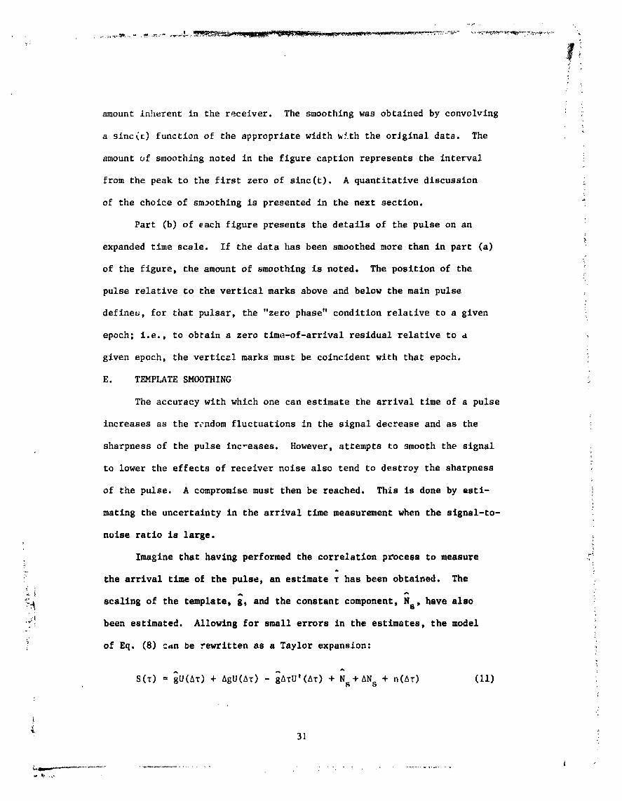
Imagine that having performed the correlation process to measure .A
i: the arrival time of the pulse, an estimate T has been obtained. The
i , have also_ scaling of the template, g, and the constant component, Ns
_I been estimated. Allowing for small errors in the estimates, the model
_ of Eq. (8) cdn De rewritten as a Taylor expansion:
A
S(T) = gU(AT) + AgU(AT) - gATU'(A_) + Ns+AN s + n(AT) (Ii)
1980024809-039
I I
(a)
_l_'r_" r_" '"T"_ I O'0 P/2 0 80ms
Figure 6. The template of PSR 0031-07: (a) P = 0.943 sec;(b) Expanded tlme scale
I I
(a)
_ 0 P12 0 40ms
_- _ Figure 7. The template of PSR 0329+54: (a) P = 0.715 sec|
.... (b) Expanded time scale
1980024809-040

(0) (b)
I I0 P/2 ,0 i3ms
Figure 8. The template of PSR 0355+54: (a) P = 0.156 sec. The pulse
has been smoothed by a window 160 psec wide. (b) Expandedtime scale
1o) (b)
)
i'
.. -P/2 6 -180ms 60ms
Figure 9. The template of PSR 0525+21, (a) P = 3.745 sec. The pulsehas been smoothed by a window 2.2 ms wZde. (b) Expandedt
time scale
1980024809-041

,f
I I
(o)
L ........ _, .., .... j_ .Ld 0
I • I0 PI2 0 120ms
Figure 10. The template of PSR 0628-28: (a) P = 1.244 sec;(b) Expanded time scale
I I
(o) (b)
I I0 P/2 0 40ms
Figure ii. The template of PSR 0736-40: (a) P = 0.374 se¢;(b) Expanded time scale
34
1980024809-04;

°
I I
(o)
o I .... t _.... - I o 'I I "
0 PI2 0 15m$ ;
Figure 12. The temptate of PSR 0823-26: (a) P = O..531 sec;(b) Expanded time scale
!
I I
(a) (b)
o-_ ---J " F -) -----I-oI I _0 PI2 0 6 ms
Figure I I. The template of PSR 08]3-45: (a) P = t).OSq ,';ec;(b) Exl)anded ti-me scale
35
1980024809-043
I(a) !
j :I I0 P/2 0 _5ms #
Figure 14. The template of PSR 0950+08: (a) P = 0.253 sec;(b) Expanded time scale
I I
(a) (b)
I I ,0 PI2 0 40ms ,_
Figure I5. The template of PSR 1133+16: (a) P = 1.188 sec;(b) Expanded time scale
1980024809-044
I I
(a) (b) \'"-"_"-I........UL-:':"-'-.... ""_',l"....' _ L_Or- ," -,--_---I....• ,--, -.--1_r----_,*',_- I
I- P/2 0 - 60 ms 0 20ms
Figure 16. The template of PSR 1237+25: (a) P = 1.382 sec;(b) Expanded time scale :.
?
I I
(o) (b)
O' r ......... _ - .i..,-_ r_--,..... ......... I-" I
I0 P/2 0 15ms
Figure 17. The template of PSR 1604-00: (a) P = 0.422 sec;
(b) Expanded time sca]e ,
J_
1980024809-045
I I
(o) (b)
! _=__._.......... i 0 _0 .... _ .... _- "2.... _ 2- -- 2 - _ ,)I
0 P/2 0 20ms
Figure 18. The template of PSR 1642-03: (a) P = 0.388 sec;
The data has been smoothed by a window 230 _seewlde. (b) Expanded time scale i
• t
I I :
(a) (b) _ : _:
: Flgure 19. The template of PSR 1706-16: (a) P = 0.b53 see;Tiledata has been smoothed by a wlndow 390 psee
wide. (b) Expanded time scale
38
1980024809-046

=
I I
I I0 P/2 0 20ms
Figure 20. The template of PSR 1749-28: (a) P = 0.563 sec;(b) Expanded t_me scale
(o) (b)
!
0 ,:
0 P/2 0 20ms
Figure 21. The template of PSR 1818-04: (a) P = 0.598 see; )
(b) Expanded time scale
!
i
39
1980024809-047
_ m",-----1g
I II
(o)
0 PI2 0 20ms
Figure 22. The template of PSR 1911-04: (a) P = 0.826 sec;
(b) Expanded time scale
I I
(o) (b)
I I0 P/2 0 25ms
Figure 23. The template of PSR 1929+10: (a) P = 0.227 sec;
(b) Expanded time scale
40
1980024809-048

\
'2
I I0 P/2 0 20ms
Figure 24. The template of PSR 1933+16" (a) P = 0.359 sec; ._.(b) Expanded time scale
j-
I I0 P/2 0 25ms
Figure 25. The template of PSR 2016+28: (a) P - 0.559 sec;
(b) Expanded t£me scale :_
41
1980024809-049

l-
i rI I 1.
(a)
0 I _ .... - .JL__ , It.... -; :1 0 :f I0 P/2 0 25ms
Figure 26. The template of PSR 2021+51: (a) P = 0.529 sec; _"(b) Expanded time scale _ ,
t ,
I
I I
;..._ -P/2 0 -120ms 0 30ms/ ,
Figure 27 The template of PSR 2045-16: (a) P = 1,96 sec.
The data has been smoothed by a window 1.2 ms wide.
(b) Expanded time scale i
!
42
1980024809-050
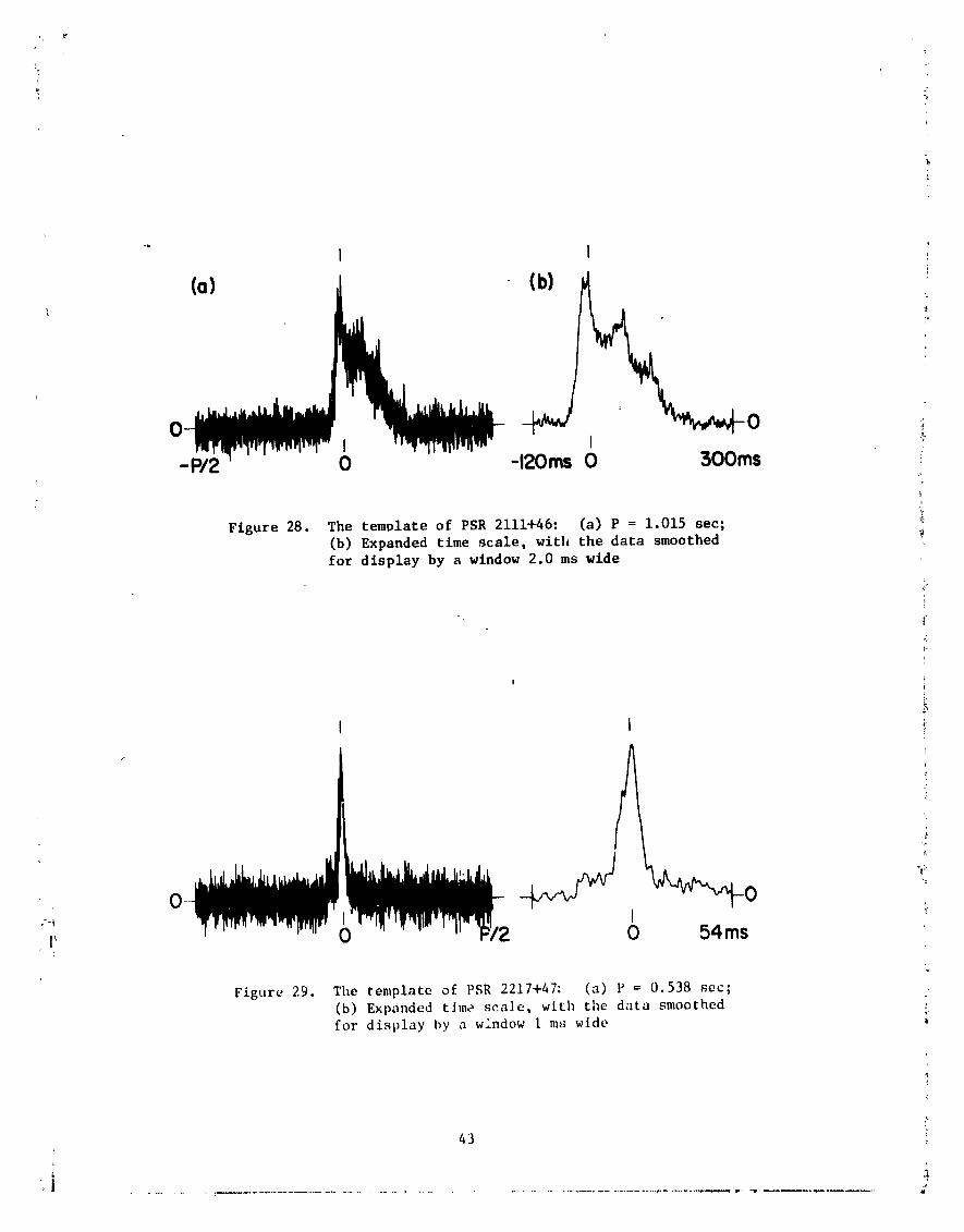
Figure 28. The template of PSR 2111+46: (a) P = i.O15 sec;(b) Expanded time scale, with the data smoothedfor display by a window 2.0 ms wide
(
!
,},
J !
¢
i' 0 0 54ms
Figure 29. The template of PSR 2217+47: (a) P = 0.538 sec;(b) Expanded tima scale, with the data smoothed
for display by a window i m,_ wide
43
I
1980024809-051
where the prime denotes a derivative, and
Ag = g - g, ANs = Ns - Ns and A_ = _ - T
Substituting Eq. (ii) into Eq. (9) yields the mean square error
A
in using estimates g, Ns and _ instead of the mean values g, Ns and T. _ •
Minimize the mean square error with respect to AT to obtain i ;
_.---j_ 2 AgU(AT) - gA'rg' (AT) + _Ns + n(Aa) i"0 _
where :"
6
U' --dU/dt, U'' = d2U/dt 2, etc. The integration is over one full '(
pulse period. Collecting terms, we make use of the following facts:
(i) U(O) = U(P) --0
(2) u'(o) .-- u'(e) = o
I'(3) n d'r = n(O) - n(P) = 0
and
(4) fnn' d_ _ 0
Then
IJ'n dr\
A'I-'_ (12) ;
" f ,)2.... g (U d'r
where terms of the order Ag/g have been omitted, iii
Since
E{A_}-fu' E{n}dT/_f(u')2 dT= ,_,
44
1980024809-052
then
EIfU'(s) n(s) dsfU°(q) n(q)dq}02 = E{Ar 2} =
_2 (u')2 dr
or _i
'(s) U°(q) Rn(S - q) ds dq2 :
O =
' [i_2 (u'12dr
?
where Rn(Ar) is the auto-correlation function of the random fluctuation2
n(t). Rn(0) ffi on. If Rn always decreases significantly before U' can
change significantly, then this result r_ains independent of the post-
detection bandwidth. Measuring tilevariance of the fluctuations in a
region not containing the pulse, we can _ite
(U')2 _
The denominator is corrected for contributions to U' from random fluc-
tuations. The expected standard deviation aF oclated with T is then or.
- The expression for oT satisfies our intuition with respect to how '
_} well z can be measured for a given signal-to-noise ratio (g/On) and a
., given pulse sharpness (measured byf(V')2 dz). A test of Eq. (13) was
performed which dia not rely on intuit_on. The, extremely noise-free
Lemplate for PSR 0833-45 was used as the basis for producing I00 records
of simulated data. A random number generator was used to superimpose
uncorrelated fluctuations onto the original template. Equatlon (13) was
45
1980024809-053
|;
12
used to choose the variance on given that o = 5 _sec. The sharpnessT
f cu,)2dr is known from the template, and g = 1 in this case.
Would the correlation method define a random process _ from the
I00 simulated data records wlch the correct standard deviation? It did, j_
The true value of z was known in this test, and the standard deviation I!
of the estimates _ about the expected value T was 5.2 _sec. !:!
The templates were smoothed to the resolution where or stopped i?
decreasing due to a lower un and began increasing due to loss in sharpness I_
of the pulse, t!F. CENTRAL SPIKES i
Occasionally, the pulse strength in some of the weaker pulsazs _
ebbs to the point of invisibility (a S/N ratio of i or less), even aftor
an hour of integration. In these data records the template seeks out !
the stronger, sharper random fluctuation,. The resulting estimate of T
represents the position in the data array of one of the larger noise
spikes. In superimposing data records to produce a template, a narrow
central spike was formed. 7
The central spike phenomenon was observed in the templates for
PSR 1818-04 and PSR 2111+46. The spike was removed by placing in the _.
central nine array locations a random process with a mean computed from t"
the eight neighboring values. The variance was set equal to that of the i_i
pulse-free portion of the array.
G. DEFINING THE ZERO-LEVEL
Defining the zero-level of the pulsed radiation is straightforward
in the cases where the puL_s are narrow and confined to one window. !:
This is not to say that the radiation between the pulses is not in part i_,
pulsed and associated with the pulsar. In most cases, however, the I_I "
!,
4b _,:
¢
1980024809-054
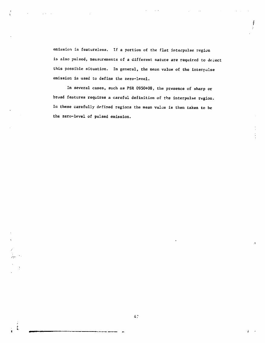
emission is featureless. If a portion of the flat intecpulse region
is also pulsed, measurements of a different nature are required to de_ect
this possible situation. In general, the mean value of the interp_ise
emission is used to define the zero-level.
In several cases, such as PSR 0950+08, the presence of sharp or
broad features requires a careful definition of the interpulse region.
ILl these carefully d_fined regions the mean value is then taken to be
the zero-level of pulsed emission.
47+
1980024809-055

SECTION V •
ESTImaTING THF PULSE ARRIVAL TIME
Each data record on magnetic tape presents an opportunity to
measure the arrival time of a received pulse relative to a given epoch.
The measurement is completed by correlating the appropriate template
(Figures 6 through 29) with data records represented by Figure i. The
correlation process leads to an estimate of the maximum cross-correlation
coefficient. However, the coefficients occur only every Pa/5000 seconds7
of delay, so interpolation in the neighborhood of the largest coefficient
is required to obtain the best estimate of the delay corresponding to the
true maximum of the coefficients. The value of the largest correlation
coefficient and an estimate of the random fluctuations due to receiver7
noise are u_ed to estimate the uncertainty in the time delay.
A. THE CORRELATION PROCESS
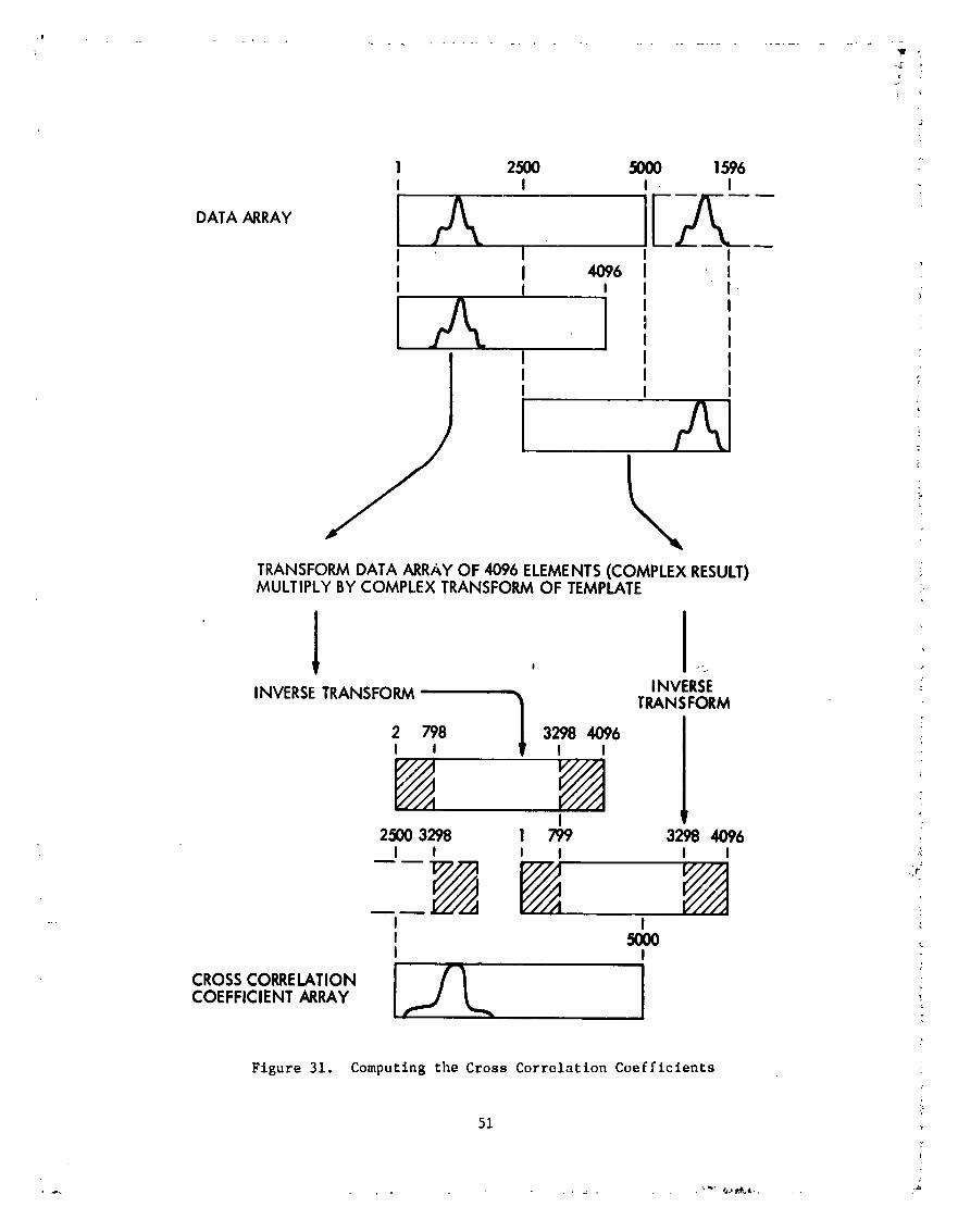
The data records are 5000 words long. Two arrays of 4096 words
each are c_nstructed to allow easy use of the FFT algorithm. The two
separate results, each 4096 words, are combined to yield one 5000-word
array of cross-correlation coefficients.
The template is shifted in position before transformation, as
shown in Figure 30. The time within each pulse corresponding to th____ee
arrival time of the pulse is, in practice, tiletime marked "0" in Fig- _,
ures 6 through 29. Each template is shifted circularly until this time
occurs in the first word of each array. Hence, the position of the
largest correlation coefficient _.'illbe the estimate of the arrival time
of that particular pulse. In addition, this shift keeps the size of
the imagi_,ary component of the transformed template to a minimum.
1980024809-056

_t
1 2048 4096
I I
TEMPLATE
ARRAY
SHIFT
TRANSFORM
REAL
TRANSFORMEDARRAY
IMAGINARY
!
Figure 30. Shifting and Transforming the Template i
J
49
J,
I
1980024809-057

obtained when no smearing is present represents a bias that can be
estimated and removed. The bias is estimated by first calculating the
expected arrival time based on the model of the pulsar, and then compar-
ing that with the arrival time expected for a pulsar with a constant#
7
period and constant Doppler shift. The meaLl of the differences is the
estimate of the bias.
The expected arrival time tk of the kth pulse arriving after the
starting epoch t o is given by
t k = tbk +_ d(t k) - d(t 0) (15)C "
where tbk is the elapsed time between k pulses at the barycenter of the
solar syatem, d(t) is the distance of the received wavefront from the
barycenter, and c is the velocity of light. Expanding the barycentric
pulse period P(t) in a Taylor series about to, _
P = P0 + P0 (t - tO) + _0 (t - t0)2/2 + 0iP t3)
It can then be shown that
tbk _ k PO + k2 PO PO/2 + O(k3 P) (16)
The quantity d(t) can be replaced with the scalar product -r (t) ia
•Up(t), where ra(t) is the position vector of the antenna relative to
the barycenter at time t. The unit vector I_ is the direction vector i'P
of the pulsar as seen from the barycenter. Referring to Figure 34, note
that l_al = a - 1 AU, and R/a >> i. Usi,_g the facts that
Y - -a cos e - d
2(R-d)Y = X2 + y2
and
X2 + y2 . Z2 = d2 + a2 + 2ad cos e,
, /
2_
1980024809-058
.I
1 2500 5000 1596I I I- I
I I i II 4096 1 _
I I I I I.
IA I' 'I I• I I
I I ::
i
v
TRANSFORMDATA ARRAYOF 4096 ELEMENTS(COMPLEX RESULT)MULTIPLYBYCOMPLEX TRANSFORMOF TEMPLATE
INVERSETRANSFORM INVERSE
TRAN:,FORM .2 798 3298 4096 .:I I I I
N N2500 3298 1 799 3298 4096I I I I I I ._
--" I II 5000 ,I
CROSSCORRELATIONCOEFFICIENTARRAY
Figure 31. Computing the Cross Correlation Coef[iclents
1980024809-059
DATA _,'w"_ .... ,,mr'_..... "r.',-,,','r'"_'..-,-r-,-_, - -.-- "r'.'.r-'-,....... '_1(PSR 1818- 0427 JAN 1970)
16h 58 mO0 • (UTC )
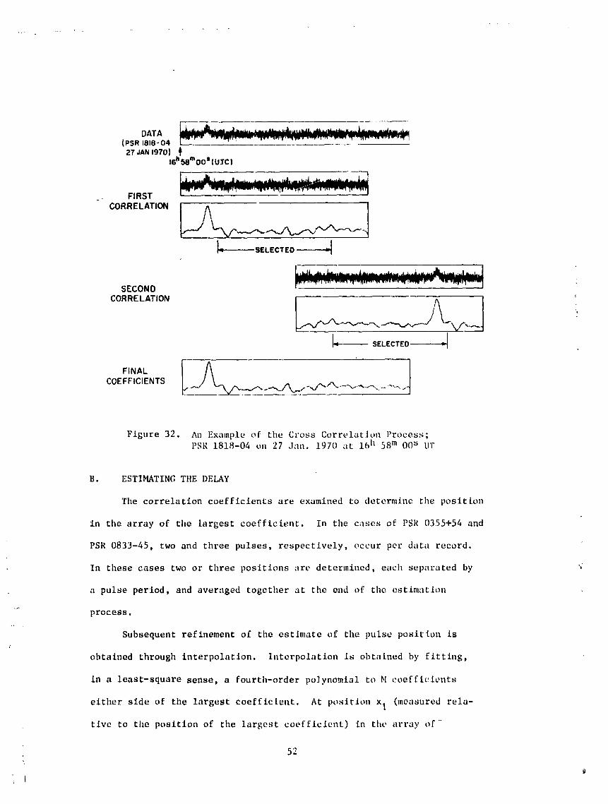
Figure 32. All Example of tileCross Correlation Process;PSR 1818-04 on 27 Jan. 1970 at 16h 58m O0s UT
B. ESTIMATING THE DELAY
The correlation coefficients are examined to determine the position
in tilearray of the largest coefficient. In the cases of PSR 0355+54 and
PSR 0833-45, two and three pulses, respectively, occur per data record.
In these cases two or three positions are determined, each separated by ",
a pulse period, and averaged together at the end of the estimation
process.
Subsequent refinement of the estlmate of the pulse position is
obtained through interpolation. Interpolation is obtained by fitting,
In a least-square sense, a fourth-order po]ynomial to M coefficients
either side of the largest coefficient. At poslrlon xI (measured rela-
tive to the position of the largest coefflcient) in the array of-
52
1980024809-060
4
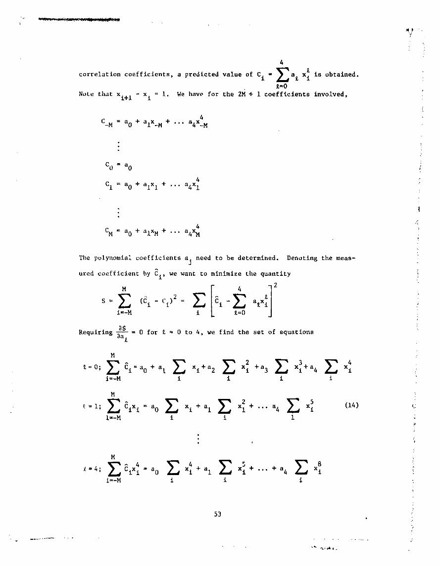
correlation coefficients, a predicted value of Ci = _a£ x£i is obtained.
Note that xi+ 1 - xi = I. We have for the 2M + 1 coefficients involved,
4
C_M = a 0 + alX_M + ... a4x_M
= ;C0 a0 f
4
C1 = a0 + alxI + ... a4x1
•
4 ::
CM = a0 + alxM + ... a4xM •
The polynomial coefficients aj need to be determined. Denoting the meas-
ured coefficient by Ci, we want to minimize the quantity
S = (Ci Ci)2 = Ci a£xi
i=-M £=0 o
8S ,:
Requiring 8a£ 0 for £ = 0 to 4, we find the set of equations
M
£=0; E Ci=a0 + al E xi+a2 _ x2i +a3 _ x31+a4 _ x4i /i=-M i i i i "
M ._
_ =i; _ Cixi --ao Z xi + al _ x21+ ''" a4 E x_ (14) ,:I=-M i i 1
e
.e S
j
M
i=-M i i i :
53. j
1980024809-061
!
Since the xi occur at uniform intervals, the sums of odd powers of xi are
zero, and the sums of even powers of x. are precomputcd for each pulsar.
The size of M is chosen separately for each pulsar. Within the range
x_M < xi < XM, the fourth-order polynomial provides a good fit to the
correlation coefficients obtained when the template is correlated with
itself.
The system of equations in Eq. (14) is solved for the polynomial
coefficients a£. The curvature of the resulting polynomial is computed.
A positive second derivative indicates a distortion due to a low signal-
to-nolse ratio, and the interpolation is not attempted. Otherwise, the
position x at which the polynomial peaked is determined. Then, steppingP
in intervals of 0.01 between x -I and x +i, the refined estimate xd ofP P
where the polynomial reaches its peak is determined.
The arrival time t of the first pulse occuring after the starta
time ts is readily calculated. The separation between data array eleme,'=s
is Pa/5000 seconds. Hence, ta = ts + xd Pa/5000.
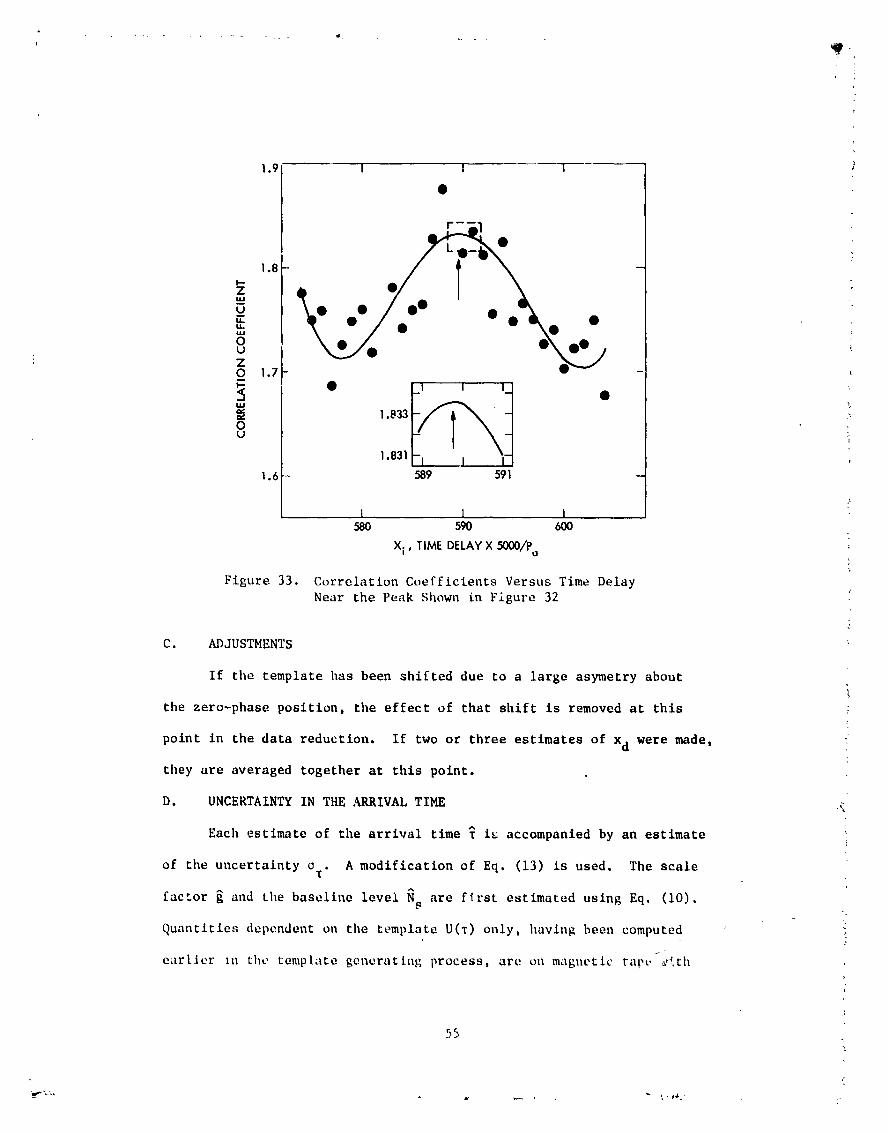
The interpolation performed near the peak coefficient in Figure 32
is presented in Figure 33. The measured values of the cross-correlatlon
coefficients (solid circles) are displayed versub the corresponding array
location, which is proportional to time delay. The solid curve is the
polynomial resulting from the least-squares fit. The pea of the poly-
nomial is near x = 589.0. The region near this value of x is enclosed
by the broken box, and reproduced on a finer scale in the inset. Pro-
' gressing from x = 589 to x = 590 in steps of 0.01, the peak, denoted
by the vertical arrow, is found at xd = 589.79.
54
1980024809-062
!.9 I I I
I1.8 -
Oo •
o\o.., i1.7 iv - ;
,-, 1.833 :,
°u ._
1.831/I I I|1.6 - 589 591 -
I l I580 590 600
X i , TIME DELAY X 5000,/Pa
Figure 33. Correlation Coefficients Versus Time Delay
Near the Peak Shown in Figure 32
C. ADJUSTMENTS
If the template has been shifted due to a large asymetry about
the zero-phase position, the effect of that shift is removed at this
point in the data reduction. If two or three estimates of xd were made,
they are averaged together at this point.
D. UNCERTAINTY IN THE ARRIVAL TIME ,;
Each estimate of the arrival time _ i_ accompanied by an estimate
of the uncertainty or. A modification of Eq. (13) is used. The scale
factor _ and the baseline level Ns are f_rst estimated using Eq. (I0).J
Quantities dependent on tile template U(T) only, having been computed t
earlier in the template generating process, are on magnetic tal,L. _'Ith
55
1980024809-063

the template itself. Note that the quantity J S(t)U(t - _) dt is merely
the maximum correlation coefficient. The root-mean-square (rms) noise
level o includes a contribution by the template. The denominator ofn
Eq. (13) is another quantity computed earlier.
56
1980024809-064

SECTION VI
GEOCENTRIC ARRIVAL TIMES
Now that the arrival time of the pulse has been measured relative to
an epoch defined by _ particular clock, it is time to consider referring
these station arrival times to the geocenter. There are several correc-
tions which must be applied to the measured arrival time before useful
geocentric results are obtained: (a) A bias in the arrival time, caused
by the smearing of the pulse during superpositioe, must be estimated and
removed; (b) the geometric correction, changing the spatial reference _:
from the antenna to the geocenter, must be applied; (c) an extra delay
• must be removed which is caused by using frequencies lower than 2388 Mliz;
(d) a small annual effect caused by the interaction of the Doppler and
dispersion phenomena must be removed; (e) the clock epochs used in the
measurements must be expressed as Coordinated Universal Time (UTC) epochs;
? (f) UTC epochs must then be expressed as ephemeris time (ET) epochs. The
result is then the arrival time that would have been obtained had the
measurement been performed et the geocenter using a clock running on
ephemeris time.
A. CORRECTION FOR PULSE SMEARING
A sm_ll amount of smearing is inevitable as the received pulses
are superimposed. The Doppler shift caused by Earth's rotation and r
orbital motion changes over the interval of integration. Also, differ-
ences can exist between the actual pulse period and the assumed period.
The result is a slow drift in the pulse phase -elative to the starting
epoch, causing the centroid of the integrated signal to drift forward
or backward in time as pulses are superimposed. The difference between
the phase of the centrold of the superlmposed pulses and tllephase
57
1980024809-065
obtained when no smearing is present represents a bias that can be
estimated and removed. The bias is estimated by first calculating the
expected arrival time based on the model of the pulsar, and then compar-
ing that with the arrival time expected for a pulsar with a constantn
period and constant Doppler shift. The meaLl of the differences is the
estimate of the bias.
The expected arrival time t k of the kt h pulse arriving after the
starting epoch tO is given by
t k = tbk +_" d(t k) - d(t 0) (15)
where tbk is the elapsed tJme between k pulses at the barycenter of the
solar system, d(t) is the distance of the received wavefront from the i
barycenter, and c is the velocity of light. Expanding the barycentric
pulse period P(t) in a Taylor series about to,
P = Po + PO (t - tO) + _0 (t - t0 )2/2 + 0iP t3)
It can then be shown that
tbk = k PO + k2 P0 P0/2 + O(k3 P) (16)
The quantity d(t) can be ceplaced with the scalar product -r (t)a
•Up(t), where ra(t) is the position vector of the antenna relative to
the barycenter at time t. The unit vector U is the direction vectorP
of the pulsar as seen from the barycenter. Referring to Figure 34, note
that I_al = a ~ 1 AU, and R/a >> 1. Usi,lg the facts that
Y = -a cos O - d
2(R-d)Y = X2 + y2
and
X2 + y2 = Z2 = d2 + a2 + 2ad cos 8,#
'_"_ 58
1980024809-066

\ \\ \\ \t
I "PULSAR y
-- i/, j,<
}
I _ I .:/ /
/
R I
Figure 34. Geometry for Calculating the Phase Drift
the distance d becomesJ
d=-a cos O =-r •a p
where R/a >> I. (The smallest value of this ratio is about I07.)
Consider the arrival time obtained if P(t) - P over the entirea
interval of integration. Suppose there is a delay of £ pulses from the
time the timing pulses are started to the time when the data collection
,f
is started (usually a few seconds at most). Then M groups of N pulses
_ (usually 500) are superimposed, with n pulses elapsing between groups
to allow for a vlsua] display of the progress of the observation. Fig-
ure 35 displays the nu_lerology used in counting these pulses. Under the
; 59 t
1980024809-067

m- 1 m= 2 m=M
' II I"*'----'f'--AAAAA_ AAAA AAAAA ,,...t
o N N N
Figure 35. Nomenclature for Enumerating Pulses
assumption of a constant period, the arrival time tak of the kth pulse
after the start epoch to is
= = kPtak [£ + J + (N + n)(m - i)] Pa a
where j is the pulse in question in the m th block of N pulses, and Pa
is the assumed constant period. (The synthesizer frequency fs used in
the observation, as per Figure 2, is 106/Pa .)
The mean of the difference tk - tak is given by
M N
- i - kPa)E {tk takl = tk- tak" _ E E (tk
m-i J=l
Let 5 = tk - tak, representing t>e bias caused by the smearing. Sub-
stitutlng Eqs. (15) and (16) into the expression fo: D yields
D - NM _ {j + £ + (N + n)(m - i)} +--_-_ (17)m=l J=:l m=l ]=i
M N
{J + £ + (N + n,(M - 1)}2 + _-_ {d(t k) - d(to)}
rn"lJ"l
,. 60
1980024809-068
!
The mean of the distances d(tk) can be replaced by the distance near the
midpoint of the range of j, yielding for the third term of Eq_ (17),
m=l
Performing the indicated s_mmatlons, Eq. (17) becomes
D = [_--+ £ + (N + n)(M - i)] (P0-Pa)2 _.
2
+TPoPo I IN_+, +I _N + n,(M- 1,.]+2 (N2- I)+ _N+12n)2 (M2- 1_ Ii (18) :.
"It I ,-,1 E ra(tO) '- c-_ ra + E + (N + n)(m - i) -m=l
It has been assumed that the signal strength is constant over the range
of k. Large fluctuations cause Eq. (18) to be in error, and if the drifti
is large, the results may be _eJected.
The expression derived above for the drift is applied te all the
data. In all cases, N = 500. The delay £ is usually O. The plot time
n is equivalent to 30 seconds before Julian date 2440195.5, and 17 sec-
onds thereafter. The numbe" M of 500-pulse integrations varies depending
on pulse strength, ranging from the equivalent of a few minutes to over
two hours.
The Jet Propulsion Laboratory ephemeri_ DE 96 is used to compute
bar_ en=ric positions r . One major export from this observing programa
is ephemezis independent, geocentric arrival times. However, the drift
correction is needed, and is best done by the observer early in the
reduction process. The use of a different ephemeris of similar quality
61
1980024809-069

will not change the corrections of Eq. (18) significantly. _ large drift
correction is on the order of a few milliscc'unds, and a velocity differ-]
ence between two ephemerides of greater than 0.i percent would be required
to produce a i ysec change in the drift estimate, fhis is usually less
than the error estimates encountered in these measurements. Note also
that this correction is dependent on a good knowledge of the pulse period
and its derivatives. These have been well-determined in a separate data
analysis effort.
The sum of the barycentric position vector of the geocenter a_Id
the geocentric position of the antenna, rg, yields ra. The computation
of _ is discussed in the next section. The direction vector U isg P
derived from a model-fitting procedure, which is beyond the scope of
this report. All the pulsar positions used here are known to at l_ast
I arL-sec, an error that will pcoduce a geocentric _rrival time error
of 0.i _sec or le_s.
An example of phase drift and the subsequent correction for the
effect is shown in Figure 36. Sixteen groups of 500 pulses of PSR 0833--45
were examined separately to estimate T. The solid circles represent these
estimates relative to the estimate for m = i. The line through the solid
circles represents a fit-by-eye to the linear drift. The triangle is
the result of examining the accumulation of the 16 blocks of data. As
one would expect in a well-behaved situation, this estimate of T has ,._
drifted about one-half the distant _rom "0" as the estimate for the
m = 16 case alone. This line through the triangle and the zero forl
this example (0 at m = I) delineates the hypothetical drift one would
find in examining ar ,n,ulation of the preceding blocks of data. The
quantity D, der_'ed from Cq. (18), is the amount the result represented
1980024809-070

3 I I l
Figure 36. An I(xample of Drift in tile Phase of I'SR 0833-45on 1 Dee. 1968 at llh O0m O0s (UT)
by the triangle is shifted to correct for drift. Note that by shifting
the datum down by D ms_ it is nearly in line with the intersection of
the dashed 1._ne and the m = 0 axis. In a later analysis the resulting
was found ae only 15 psee away from the arrival time predicted by a
smooth model, which was fitted to several months of data.
B. AhV£ENNAPOSITION
The referral of the measured arrival time to the geocenter requires
- -Upg/Cthe addition of th_ time delay r • , where r is the geocentric
g g
position of tileantenna and U is the geocentric direction vector ofPg
tilepulsar. In practice U _ U . The coordinate system used here isPR P
the right-handed rectangular system (×, v Z). Tilt' cot,rdinate X i,_ itl
tilt, dll'ectioll of ()|1 I_igl_t ._qt'tHlsion (P_) at ]tt_('_.O. Tilt' _tatitm p,,sit ion
,It ,l ]',tr[ [t llt,.l '_'l't' t[,,,,'h i:, t'd]cul.ttt'd J'l't'l;1 th, ;iut:' ll,q t't't'l't]i;I,ttt", J;:
1980024809-071

Table 5 and tile knowledge of tile Greenwich Hour Angle (CHA). The station
coordinates are a version of Location Set (LS) 44, which are based on the
ephemeris DE 96 (Ref. 19). The GHA is computed as outlined in Table 6
(see Ref. 20).
Table 5. Geocentric Antenna Coordinates
West
Longitude _ Latitude _ Radius R
Antenna (deg) (dog) (km)
DSS ii (26ra) 116.849390 35,20804) 6372.011
DSS 12 (34m) 116.805462 35. 118665 6371. 994
DSS 13 (26m) 116.79_863 35.066546 6372. 117
DSS 14 (64m) 116.889507 35.170847 6366. 227
DSS 62 (26m) 4.367811 40. 263145 6369. 963
DSS 63 (64m) 4.247991 40.241318 6370.048
Table 6. Relations Used in Computing the GHA of anObserving Station
At the epoch d + SEC/86400,
10-13(:HA= 100.0755426 + d(0.985647346 + 2.9015 x d)
+ 0 SEC 4. _ cos(c) degrees
where: (1) d = Julian days pas_ 2433282.5
(2) SEC seconds past 0 b= on day d
10 -13(3) 0 = 4.17807417 x 10⁻³/(1+5.21 x d) deg/sec
' (4) _, the nutatlon in longitude, is taken from
: ephemeris DE 96
(5) _ --4.09205684 x 10⁻¹
+ T[-2.28534 x 10⁻⁴ + T(-I.Sx 10-8+ 8.7 x 10⁻⁹)] radlans
where T Is in Julian centuries of 36525 days past
2433282.5.
64
1980024809-072
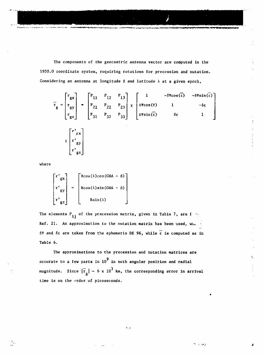
The components of the geocentric antenna vector are computed in the
1950.0 coordinate system, requiring rotations for precession and nutation.
Considering an antenna at longitude 8 and latitude _ at a given epoch,
rg = rgy I P21 P22 P22J X 4_cos(-6) 1 - g
'32 '33J LA'sinG)
p! _ /
gXl <
Xlr' [gYl
t
Ir'
. gzj
where
"r' - -Rcos(A)cos(GHA - 6)"gx
r' = Rcos(l)sin(GHA - 6)gY
r'gzj _ Rsin(_)
The elements Pij of the precession matrix, given in Table 7, are f .....
Ref. 21. An approximation to the nutation matrix has been used, wh__w
6_ and _e are taken from the ephemeris DE 96, while e is computed as in
Table 6.
The approximations to the precession and nutatlon matrices are
accurate to a few parts in 109 in both angular position and radial
"' magnitude. Since Irgl _ 6 x 10³ km, the corresponding error in arrival
time is on the order of picoseconds.
I:)
I
1980024809-073
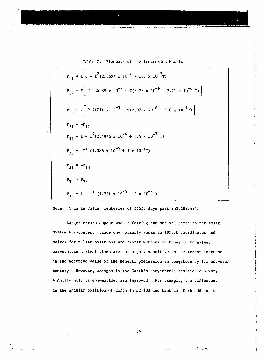
Table 7. Elements of the Precession Matrix "
PII = 1.0 - T2(2.9697 x I0-4 + 1.3 x IO-7T)i
_: _[__ x_0-_+_0,_x_0-__x _0-°_]
P21 = -PI2
P22 = 1 - T2(2.4976 x 10⁻⁴ + 1.5 x 10⁻⁷ T)
= _T2P23 (1.085 x 10⁻⁴ + 3 x 10-ST)
P31 = -PI3
P32 = P23
[ P33 = i - T2 (4.721 x 10⁻⁵ - 2 x IO-8T)
Note: T is in Julian centuries of 36525 days past 2433282.423.
Larger errors appear when referring the arrival times to the solar
system barycenter. Since one normally works in 1950.0 coordinates and
solves for pulsar positions and proper n_otions in these coordinates,
barycentric arrival times are not highly sensitive to _he recent increase
in the accepted value of the general precession in longitude by i.i arc-sec/J
century. However, changes in the Earth's barycentric position can vary
significantly as ephemerldes are improved. For example, the difference
in the angular position of Earth in DE 108 and that in DE 96 adds up to
1980024809-074

about 0.5 arc-sec/century.* In a ten-year observing program, the differ-
ence is then 0.05 arc-sec, similar to the errors in pulsar positions
derived from the arrival time data.
C. DISPERSION
Considerable effort was expended in the early observaLions to
obtain one frequency, 2388 MHz. This was not always possible, for
several observations occurred at 2295 and 2328 MHz. All observations
are now at 2295 MHz. Integration of Eq. (i) provides the corrections
in time to be added to an arrival time measured at F MHz to refer iti
back to 2388 _z. Performing the integration, the correction ATD becJmes
Dbl 1ATD
= F2J sec (19)2.410086 x 10⁻⁴ (2388)2
where the values of DM are fcom Table 4.
In the application of ATD to PSR 0833-45 it was found that an
addf:ional 250 _sec had to be subtracted frbm tilemeasurement when
F = 2295 MHz. No significant addendum was needed when F = 2328 MHz.
The average pulse shape must be independent of observing frequency if
the correction ATD is to be perfectly adequate. Most shapes do change
significantly with frequency, including that of PSR 0833-45, thus
creating the need to measure an addendum to ATD.
D. DOPPLER DISPERSION "\
The actual frequency of observation varies with the component of
antenna velocity laying along the direction of the pulsar. The measured
arrival time then llasa varying component since the interstellar medium
*E.M. Standish, prlwlte communication.
67
1980024809-075

!
is dispersive. TileDoppler-shifted observing freq,ency F0 is related to
the mean observing frequency F0 by
FO = F0 i + a pC
where V is the barycentric velocity of the antenna. In this situation,a
integration of Eq. 1 leads to a form similar to Eq. (19). Performing
that operation,
ATDD = DM I - i2 V U
1.205043 x 10⁻⁴ F0 1 + a pC
where ATDD , the correction for Doppler dispersion is added to the meas-
ured arrival time. Using the fact that IVa/CI < I0-4, and setting F0 =
2388 Nttz, the correction becomes
-- x %)/c :The magnitude of this yearly oscillation is abo,tt 6 bsec for
PSR 0833-45 and about 18 _sec for PSR 1933+16. This correction is not
small in all cases compared to the measurement accuracy, nor is it small
compared to the desired uniformity of the approximation to ephemeris
time.l
E. ARRIVAL TIME IN UTC _'
The epoch at which the data sampling process begins is defined by
'"_" a l-sec pulse from the station clock. A sequence of l-seco_d pulses
(clock pulses) is sent continuously via microwave link from the Standards
Laboratory at the Goldstone complex to the individual tracking stations.
Allowing for the delay over the links, these pulses define a UfC which
is within 5 _sec of UTC as disseminated by the National Bureau, of
68 ,
1980024809-076

!
Standards (NBS). The 1-second pulses generated at DSS 14, UT(DSS 14),
are kept within 5 _sec of the Standards Laboratory pulses. Therefore,
at DSS 14 the l-sec pulses are assumed to be within i0 _sec of UTC (NBS).
The l-sec pulse used at DSS 13, UT(DSS 13), is frequently synchronized
with the Standards Laboratory pulses to within i _sec. A plece-wise linear
curve approximating the deviation in this l-sec pulse from UTC(NBS) is
used to correct epochs at DSS 13 to UTC (NBS). The correction is at
most i00 _sec.
The correction equal to the width of the clock pulse at DSS 14 is
subtracted as part of this correction. (See the discussion of system
codes 2, 3, and 5, and Fig. 3.) The small correction equal to Pa/5000
is then added if appropriate.
F. CONVERSION FROM COORDINATED UNIVERSAL TIME TO EPHEMERIS TIME
Coordinated Universal Time (UTC) is an approximation to a uniform
time based on the rotati)n of Earth. Several steps are necessary to con-
vert to the truly uniform ephemeris time (ET). Of prime importance
is the correction for annual effects due to the orbital motion of the
Earth-based clocks about the Sun. The correction AET i_ given in
(Ref. 16) as
AET = 0.001658(_in E + 0.0368) sec (21)
whece E is the eccentric anomal_" of the Earth in a heliocentric orbit.#
Letting M represent the mean anomaly of Earth and e the orbitali
eccentricity,
sin E = sin M (i _ e cos M)#
69
1980024809-077
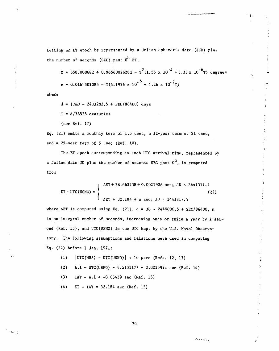
Letting an ET epoch be represented by a Julian ephemeris date (JED) plus
the number of seconds (SEC) past Oh ET,
_' M = 358.000682 + 0.9856002628d - T2(1.55 x 10⁻⁴ +3.33x IO-6T) degrees
_5 IO_7T )e = 0.0167301085 - T(4.1926 x i0 + 1.26 x
where
d = (JED - 2433282.5 + SEC/86400) days
T ffid/36525 centuries
(see Ref. 17)
Eq. (21) omits a monthly term of 1.5 _sec, a 12-year term of 21 _sec,
and a 29-year term of 5 _sec (Ref. i0).
The ET epoch corresponding to each UTC arrival time, repcesented by
a Julian date JD plus the number of seconds SEC past Oh, is computed
from
I AET+38.662738+0.002592d sec; JD < 2441317.5
ET- UTC(USNO) = ) (22)gET + 32.184 + n sec; JD > 2441317.5
where _ET is computed using Eq. (21), d = JD - 2440000.5 + SEC/86400, n _
is an integral number of seconds, increasing once or twice a year by i sec-
ond (Ref. 15), and UTC(USNO) is the UTC kept by the U.S. Naval Observa-
tory. The following assumptions and relations were used in computing i
Eq. (22) before 1 Jan. 197_:
(i) IUTC(NBS) - UTC(USNO) I < i0 _sec (Refs. 12, 13)
(2) A.I - UTC(USNO) = 6.5131177 + 0.002592d sec (Ref. 14)
(3) IAT - A.I = -0.03439 sec (Ref. 15)
(4) ET - IAT = 32.184 sec (Ref. 15)
70
1980024809-078
After Jan. 1972, the appropriate number of integral seconds is added to
the UTC epoch to obtain IAT (Ref. 15) under the assumption that IUTC(NBS)
- UTC (Bureau de l'Neure) I < i0 _sec (Ref. 12). Then ET is obtained from
ET - IAT = 32.184 sec.
G. AN EQUIPMENT IDIOSYNCRASY
The equipment problem of system code 3 requiring a correction of
-0.996550 seconds is taken into account along with the corrections
discussed _bove.
H. A TEST OF THE MEASUREMENT CONSISTENCY
The consistency of the measurements is determined by comparing the i
results using the procedures described earlier in the editing process
(Sec. III). This comparison led to the correction of 0.996550 sec for
the equipment failure, and the additional 250 _sec correction at
2295 MHz for PSR 0833-45. The question finally arises concerning the
consistency of arrival times measured at different stations. Six epochs
exist for PSR 0833-45 for which measurements were made at DSS 13 and
DSS 14 within i day of each other. Results of three of these measure-
ments showed DSS 14 results differing slgniflcaLtly from those at DSS 13.
There were, however, serious receiver tuning problems at DSS 14 at two i
of the three epochs. Of the three results showing agreement, two are
presented in Figure 37, where the difference (residual)between the
measured and predicted arrival times is presented for each Julian date
(JD) of observation (MJD = JD - 2440000.5). The agreement is remarkably
good, leading to the conclusion that no systematic differences between
DSS 13 and DSS 14 measurements remain in this data set,
71
1980024809-079
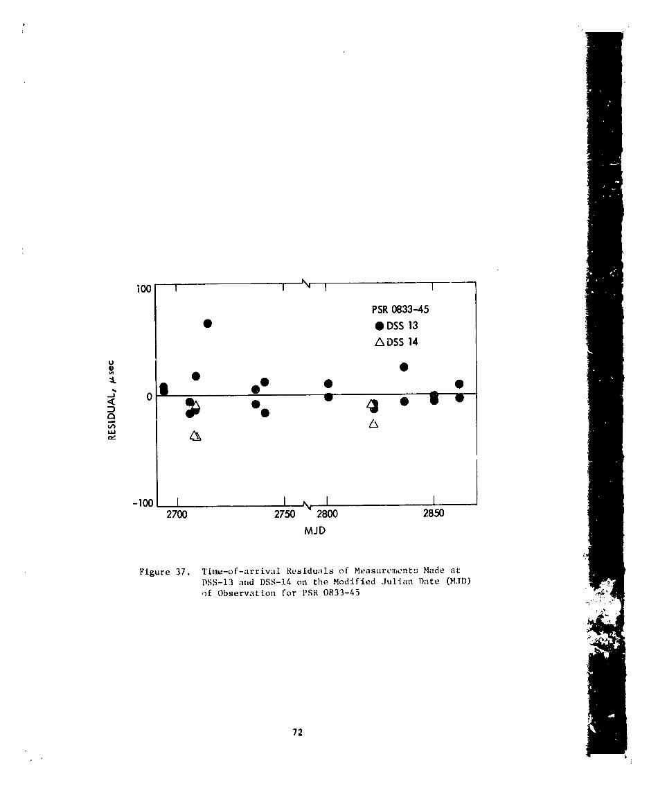
100 I I .N, I I
PSR0833-45
• • DSS13A DSS14
.__ 08 o• • _ •_ •:::, _ • II •
,,-,, _ •u.I
-loo I I N I L2700 2750 2800 2850
MJD
Figure 37. Time-of-arriwll Residuals of Measur¢,mcnts Made atDSS-I3 and DSS-14 on tileModified Julian l)ate (M.ID)
of Observation for PSR 0833-45
72
• -, I_ I
1980024809-080

SECTION VII
THE TABULAR RESULTS
An example of the observational results is presented in Table 8.
- Columns i and 2 list the ephemeris time of the pulse arrival at the
geecenter as a Julian ephemeris date and the number of seconds past
oh(ET). (Note that no complete removal of the dispersion effect has
been applied. That is, these arrival times refer to F = 2388 MHz, not
F = _.) The estimate of the expected standard deviation of the measure-
ment (defining the 67 percent confidence interval if the measurement
errors are Gaussian) appears in Column 3. In Column 4, all of the time
conversions from UTC to ET discussed in Section VI are listed. Column 5
contains the applied drift correction, while the configuration code
appears in Column 6. Barycentric arrival times are listed in Column 7
for analysts satisfied with the accuracy of DE 96.
ACKNOWLEDGEMENT
Over the course of ten years many individuals have contributed to
the success of this observing program, most of them on the staff of the
NASA Deep Space Network. Dedicated, excellent work was and is performed
in the collection of the data by G. Birkedahl, R. Genzmer, J. W. Hudson,
C. Kodak, C. Mitchell, R. McConahy, D. Rife, L. SkJervs, D. Spitzmesser,
L. Wadsworth, G. Wischmeyer, and the staff of DSS 62. Much patient
support has been contributed by R. M. Goldstein, R. R. Green,
I E.B. Jackson and G. S° Levy.
Cr[tical technical support was kindly provided by S. S. 3rokl,
C. F. Foster, R. R. Green, G. A. Morris, K. I. Moyd, A. G. Slekys,
I. Ute'_'h, :md M. Urt, t'h.
'1980024809-08 '1
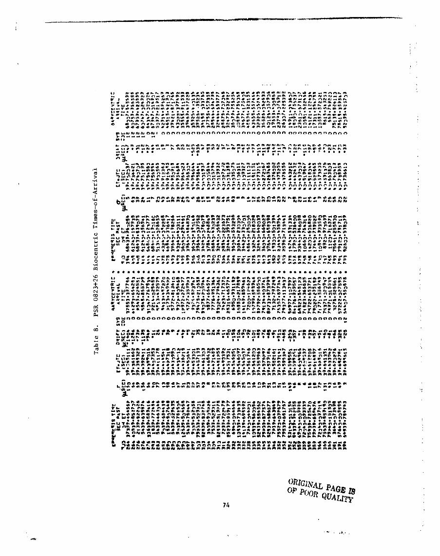
,iw • -- _.... I J ]
)
ORIG1_V,,U.,P,._GOP PO0 ,_;;'._B/B
R _uaLlTT74
1980024809-082
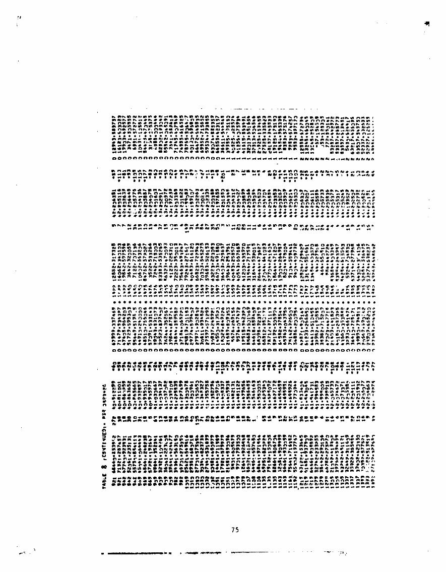
75
1980024809-083

i
1980024809-084
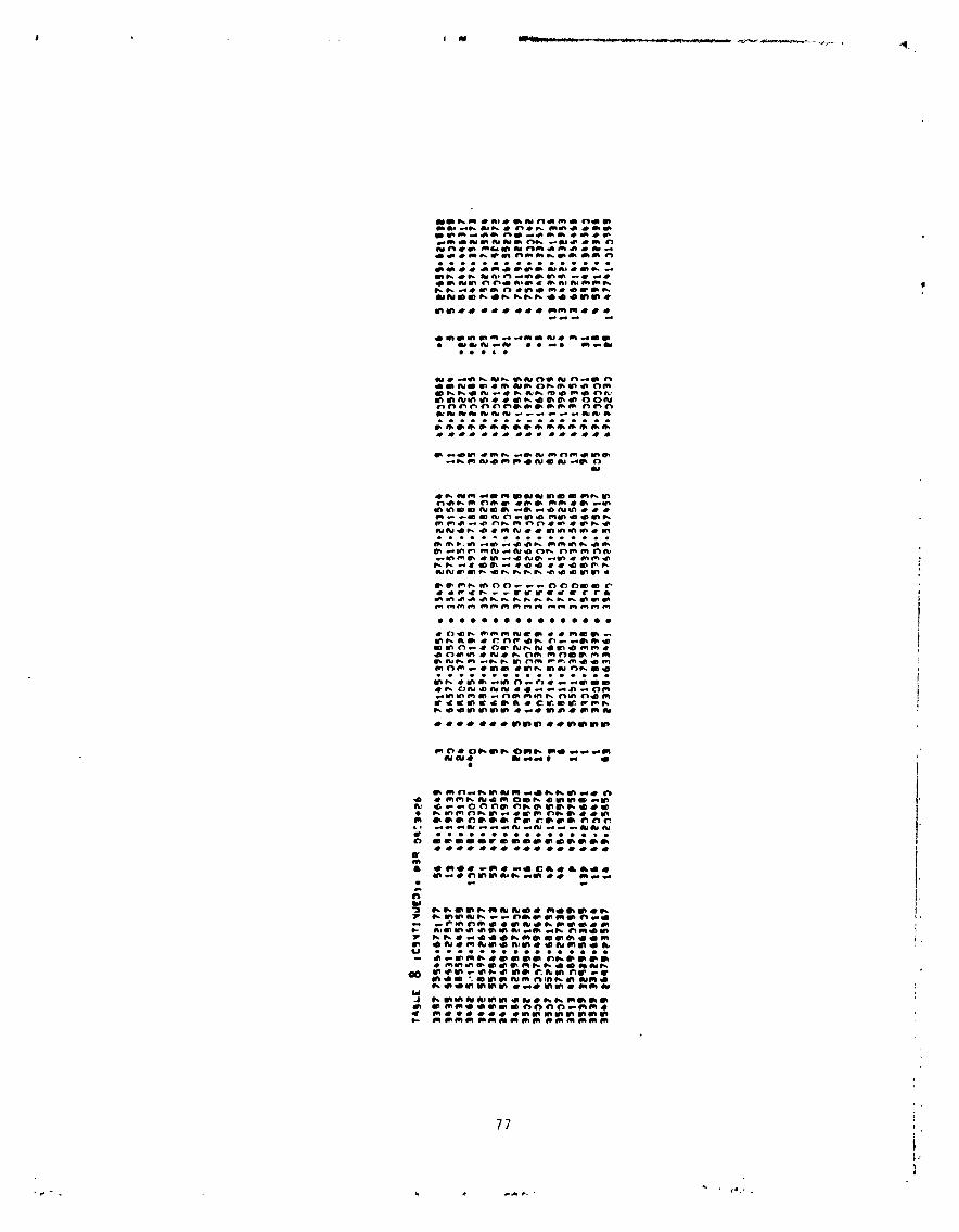
pnmm_*_.oI,,,.41_@,..• _me_, 6iIi#__po.Ii.gMim
o • I ¢ •
° 11
_a
77
t|
1980024809-085

REFI._I¢I¢NCt._S
I. tit, wish• A.• Bill, S. ,I., l'ilkington• ,1. D. I1., Sct_tt• P. F.• and
Collins• R. A.• "Observation of a Rapidly Pulsating Radio Source,"
Nature, Vol. 217, 1968• p. 709.
2. Pilkington, J. D. H.• ttewish, A.• Bell• S. J.• and Cole, T. W.,
-,i "Observations of Some Further Pulsed Radio Sources," Nature•
° • .) rVol 218 1968, p. l~o.
3. Gold. T., "Rotating Neutron Stars as the Origin of the Pulsa. ing
Radio Sources," Nature, Vol. 218, 1968• p. 731.
4. bloffet, A. T. and Ekers, R. D.• "DeEettion of the Pulsed Radio
Source CP 1919 at t3-cm Wavelengths" Nature, Vol. 218, 1968,
p. 227.
¢ Bracewel 1 , R. N. , 'l'l_e yc?_u]'ier Trans_fq_rm .m_dl tzs _Ap_plications ,
blc(;raw-llil I , New York, 1965, p. 339.
6. Foster, C. F., "Automated Pulsar Receiver," _DSN_j'y3Lgyess
R_t.j_or_t 42-20, ,let Propulsion l,aboratory, I'asadena, Cal ifornia,
April 15, 1974.
7. Slekys, A., A N.e_w_l'_tLlsa__r_'!'in:er_• ,IPl. Technica'. Report 32-1526,
Vo!. Xlll, ,let I'ropulsion l,aboratt-ry, l):lsadt, na, ('alif_ rnia,
I:el_. lq, 1973.
8. Brokl, S. S., "Automated Pulsar Data t:ollector," l)SN_J'rog_.)'es_s - i.,
i',eport 42 _.... -.), .let Propulsion l,aboratory, l'asadena, Calil't.'rnia•
Feb. 15, 1975.
q. Rt, ichlt, y, P. l'., I)owns, t;. S., nntl blorris, (;. A., "Time-Of-Arriv;ll
obst.rwltions _I Eleven Pul._ars," Aj). 3., Vol. 159, 1970, p. 1,35.
78
1980024809-086
!
10. {'ooley, l. W., Lewis, 1'. A. N., and Welch, 1'. D., "The Fourier
Transform Algorithm: Prograwming Considerations in the Calculation
of Sine, Cosine and Laplace Transform, '° J. Strand Vib., Vol. 12,
1970, p. 315.
II. Brigham, E. O., The Fast Fourier Transform, Prentice-Ilall,
Englewood Cliffs, New Jersey, 1974.
12. NBS Time and Frequency. Bulletin, U. S. Dept. of Commerce, National
Bureau of Standards, Boulder, Colorado, 1968 to 1979.
13. Daily Phase Values and Time DifFerences, Series 4, U. S. Naval
Obserw_tory, Nashington, D. C., 1968 to 197,.
14. Times Services Bulletin, Series II, No. 220, U. S. Naval
Obsecvatory, Nashington, D. C.
15. Preliminary Times and Coordinates of the Pole, Series 7, No. 210,
U. S. N:lval Obserwltory, Nashingtot_, D. C.
16. Helbourne, N. G., Mulholland, J. D., S.jorgren, W. 1,., and Sturms, :-
F. b|., Collstants and Related Information for Ast_fo_3LdJnamic Cal-
t'ul at ion.:s __ I')(_q, JPL Technical Report 32-1 306, Jet i'ropul sion
Laboratory, Pasadena, California, July 15, lq68.
17. Sturms, F. H., .Ir., _Pg_lynomial Expressions for Planetary E_uators
an__51Orbit Elements vitia Resnect to the Heart 1950.0 Coordinate
S_,m, JPI. Technical Report 32-1508, .let Propulsion Laboratory,
Pasadena, California, January 15, ',971,
18. Hoyer, T.!)., Transformat:on from Proper Time on Earth to Coordin-
ate Time in Solar S_stem Barycer, tric _pacc-'rime l:rmno of
Refcrt, nt:e, .ll'l, Tct'lulicn] _emorantltlm _3-786, .let Propulsion _J
1,ab_r,ltorv, P,l,,':ldon_l, Calift_rnin, I)oc. 1 , lqTh.?
--1r
79
1980024809-087

19. Koble, It. H,, l'ciise, t;. E., ;rod Yip, K. lq., 'tl_S44-An Improved Deep
Spawe Network St,it ion I,_cation Set for Vikinjs N;Ivig,lti_m," in becp
:.;j2et.,y_j,;_ejwt,r]K ProL,,.r,.:,;2; Ryp.W-t 4_-'" _5, .It, t l'r,_lmlsi_m l,;,b,_r.lt ,,v,
])/|s;Id¢-_ll;l, C,tliftu'ui.J, Oct. 15, ]97_.
?.(1. White, R. .1., R_)scnberg, A. 1)., l.'i:dlcr, I'. S.. il;irris, R. ,\., .lint
a_,,d_al I, N. S., SPACE -Stj_2A___L t'ryc.i:si,jt \ _Q,_wcI 1 _T_r,_j_vc.t_,:r t'r:,,_;r:,.m,
.IP! Technical l_lem(,r:mdt,m, 33-198, .Io! Propulsion l,;d)orator,.',
I'asadena, California, Jail. 15, 1965.
21. II_)ldridge, 1)., Sjmce Tra}ectorie_._.zs PrP__ram for the IBbl 7090
Quu. lfuter , .lPl, 'lechnicnl Report 3"2-'223, Rev. 1, .let l'r,qmlsion
I,;dmrnttwy, I'as/ldenn, (';llifornia, Septeml)er I, 1962.
",9 Taylor, .I. II , and H,mchester, R. N., (t)servc_ Propert ies of Ih7
Ih,lsars," Astron..I., Vol. 80_ 1975, p. 794.
_0 NA._II-JPI -COt!_l I A, C,l_d
1980024809-088


