The 0/1 Knapsack ProblemThe 0/1 Knapsack Problem
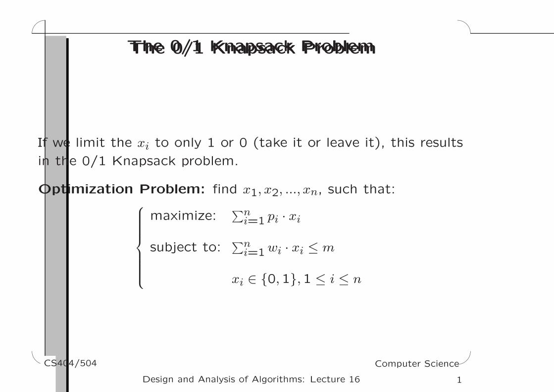
If we limit the xi to only 1 or 0 (take it or leave it), this results
in the 0/1 Knapsack problem.
Optimization Problem: find x1, x2, ..., xn, such that:
maximize:∑n
i=1 pi · xi
subject to:∑n
i=1 wi · xi ≤ m
xi ∈ {0,1},1 ≤ i ≤ n
'
&
$
%CS404/504 Computer Science
1Design and Analysis of Algorithms: Lecture 16

The Greedy method does not workfor the 0/1 Knapsack Problem!
The Greedy method does not workfor the 0/1 Knapsack Problem!
'
&
$
%CS404/504 Computer Science
2Design and Analysis of Algorithms: Lecture 16

The Knapsack ProblemThe Knapsack Problem
There are two versions of the problem:
1. “Fractional” knapsack problem.
2. “0/1” knapsack problem.
1 Items are divisible: you can take any fraction of an item.
Solved with a greedy algorithm.
2 Item are indivisible; you either take an item or not. Solved
with dynamic programming.
'
&
$
%CS404/504 Computer Science
3Design and Analysis of Algorithms: Lecture 16

0/1 Knapsack problem: the brute-forceapproach
0/1 Knapsack problem: the brute-forceapproach
Let’s first solve this problem with a straightforward algorithm:
• Since there are n items, there are 2n possible combinations
of items.
• We go through all combinations and find the one with the
maximum value and with total weight less or equal to m.
• Running time will be O(2n).
'
&
$
%CS404/504 Computer Science
4Design and Analysis of Algorithms: Lecture 16

Can we do better?Can we do better?
• Yes, with an algorithm based on dynamic programming.
• Two key ingredients of optimization problems that lead to
a dynamic programming solution:
– Optimal substructure: an optimal solution to the
problem contains within it optimal solutions to
subproblems.
– Overlapping subproblems: same subproblem will be
visited again and again (i.e., subproblems share
subsubproblems).
'
&
$
%CS404/504 Computer Science
5Design and Analysis of Algorithms: Lecture 16
Optimal Substructure of 0/1 Knapsackproblem
Optimal Substructure of 0/1 Knapsackproblem
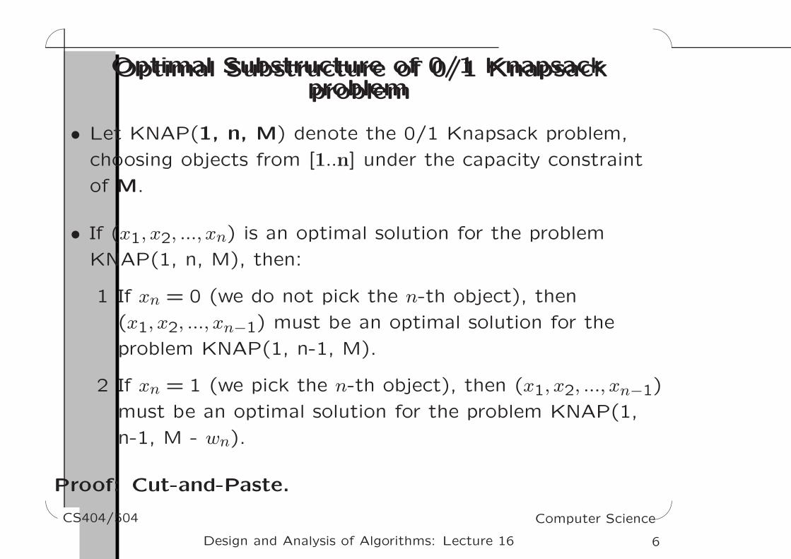
• Let KNAP(1, n, M) denote the 0/1 Knapsack problem,
choosing objects from [1..n] under the capacity constraint
of M.
• If (x1, x2, ..., xn) is an optimal solution for the problem
KNAP(1, n, M), then:
1 If xn = 0 (we do not pick the n-th object), then
(x1, x2, ..., xn−1) must be an optimal solution for the
problem KNAP(1, n-1, M).
2 If xn = 1 (we pick the n-th object), then (x1, x2, ..., xn−1)
must be an optimal solution for the problem KNAP(1,
n-1, M - wn).
Proof: Cut-and-Paste.
'
&
$
%CS404/504 Computer Science
6Design and Analysis of Algorithms: Lecture 16

Solution in terms of subproblemsSolution in terms of subproblems
Based on the optimal substructure, we can write down the
solution for the 0/1 Knapsack problem as follows:
• Let C[n, M] be the value (total profits) of the optimal
solution for KNAP(1, n, M).
C[n, M] = max ( profits for case 1,
profits for case 2)
= max ( C[n-1, M], C[n-1, M - wn] + pn).
Similarly
C[n-1, M] = max ( C[n-2, M], C[n-2, M - wn−1] + pn−1).
C[n-1, M - wn] = max ( C[n-2, M - wn],
C[n-2, M - wn - wn−1] + pn−1).
'
&
$
%CS404/504 Computer Science
7Design and Analysis of Algorithms: Lecture 16

Use a table to store C[·,·] and build it in abottom up fashion
Use a table to store C[·,·] and build it in abottom up fashion
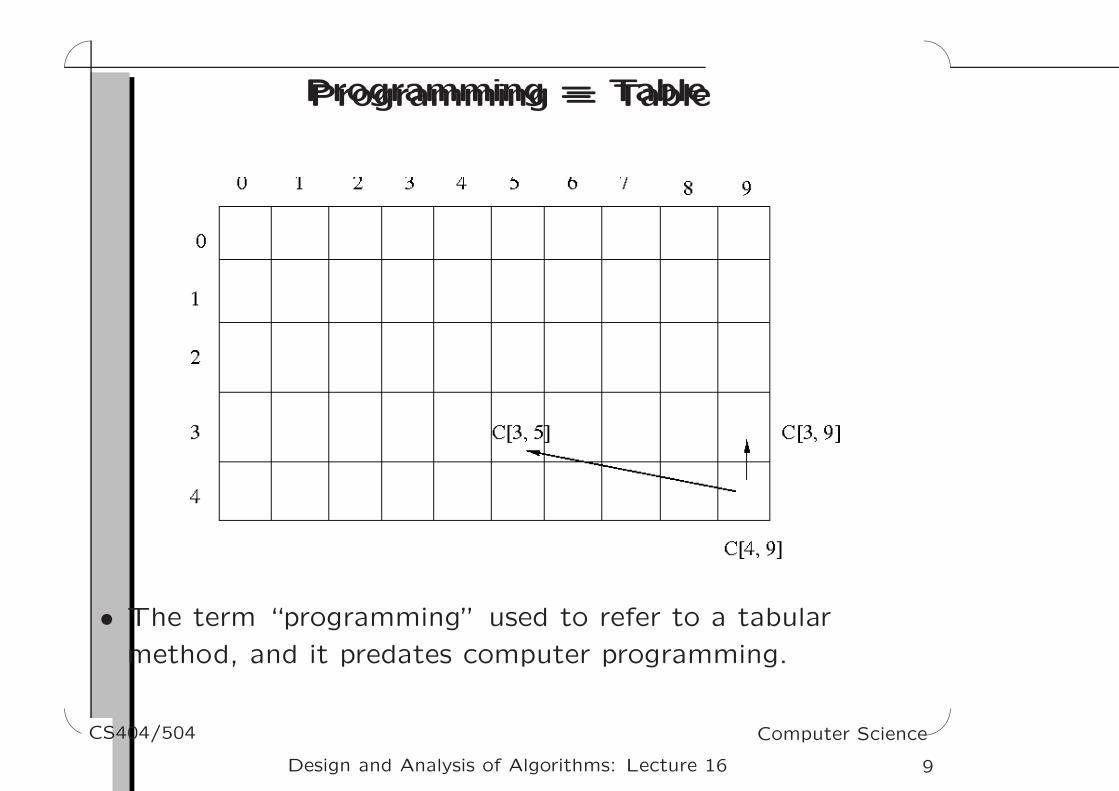
• For example, if n = 4, M = 9; w4 = 4, p4 = 2, then
C[4, 9] = max( C[3, 9], C[3, 9 - 4] + 2).
• We can use a 2D table to contain C[·,·]; If we want to
compute C[4, 9], C[3, 9] and C[3, 9 - 4] have to be ready.
• Look at the value C[n, M] = max (C[n - 1, M], C[n-1, M -
wn] + pn), to compute C[n, M], we only need the values in
the row C[n - 1,·].
• So the table C[·,·] can be built in a bottom up fashion: 1)
compute the first row C[0, 0], C[0, 1], C[0, 2] ... etc; 2)
row by row, fill the table.
'
&
$
%CS404/504 Computer Science
8Design and Analysis of Algorithms: Lecture 16
Programming = TableProgramming = Table
• The term “programming” used to refer to a tabular
method, and it predates computer programming.
'
&
$
%CS404/504 Computer Science
9Design and Analysis of Algorithms: Lecture 16

Construct the table: A recursive solutionConstruct the table: A recursive solution
• Let C[i, ̟] be a cell in the table C[·,·]; it represents the
value (total profits) of the optimal solution for the problem
KNAP(1, i, ̟), which is the subproblem of selecting items
in [1..i] subject to the capacity constraint of ̟.
• Then C[i, ̟] = max(C[i − 1, ̟], C[i − 1, ̟ - wi] + pi).
'
&
$
%CS404/504 Computer Science
10Design and Analysis of Algorithms: Lecture 16
Boundary conditionsBoundary conditions
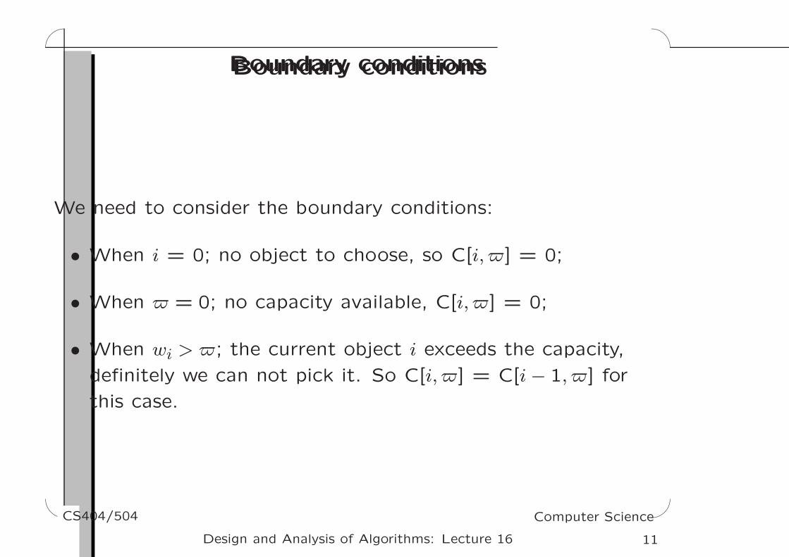
We need to consider the boundary conditions:
• When i = 0; no object to choose, so C[i, ̟] = 0;
• When ̟ = 0; no capacity available, C[i, ̟] = 0;
• When wi > ̟; the current object i exceeds the capacity,
definitely we can not pick it. So C[i, ̟] = C[i − 1, ̟] for
this case.
'
&
$
%CS404/504 Computer Science
11Design and Analysis of Algorithms: Lecture 16

Complete recursive formulationComplete recursive formulation
Thus overall the recursive solution is:
C[i, ̟] =
0 if i = 0 or ̟ = 0
C[i − 1, ̟] if wi > ̟
max(C[i − 1, ̟], C[i − 1, ̟ − wi] + pi)if i > 0 and ̟ ≥ wi.
The solution (optimal total profits) for the original 0/1
problem KNAP(1, n, M) is in C[n, M].
'
&
$
%CS404/504 Computer Science
12Design and Analysis of Algorithms: Lecture 16

AlgorithmAlgorithm
DP-01KNAPSACK(p[], w[], n, M) // n: number of items; M: capacity
for ̟ := 0 to M C[0,̟ ] := 0;
for i := 0 to n C[i, 0] := 0;
for i := 1 to n
for ̟ := 1 to M
if (w[i] > ̟) // cannot pick item i
C[i, ̟] := C[i - 1, ̟];
else
if ( p[i] + C[i-1, ̟ - w[i]]) > C[i-1, ̟])
C[i, ̟] := p[i] + C[i - 1, ̟ - w[i]];
else
C[i, ̟] := C[i - 1, ̟];
return C[n, M];
'
&
$
%CS404/504 Computer Science
13Design and Analysis of Algorithms: Lecture 16
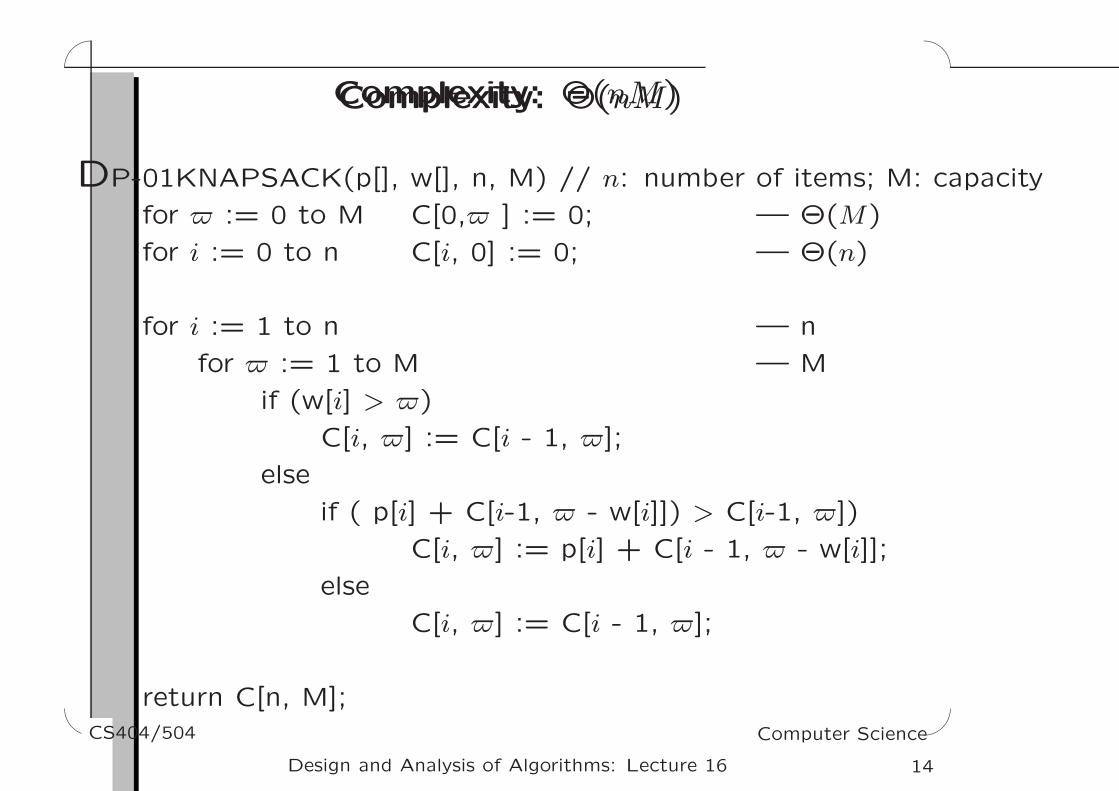
Complexity: Θ(nM)Complexity: Θ(nM)
DP-01KNAPSACK(p[], w[], n, M) // n: number of items; M: capacity
for ̟ := 0 to M C[0,̟ ] := 0; — Θ(M)
for i := 0 to n C[i, 0] := 0; — Θ(n)
for i := 1 to n — n
for ̟ := 1 to M — M
if (w[i] > ̟)
C[i, ̟] := C[i - 1, ̟];
else
if ( p[i] + C[i-1, ̟ - w[i]]) > C[i-1, ̟])
C[i, ̟] := p[i] + C[i - 1, ̟ - w[i]];
else
C[i, ̟] := C[i - 1, ̟];
return C[n, M];
'
&
$
%CS404/504 Computer Science
14Design and Analysis of Algorithms: Lecture 16

An exampleAn example
Let’s run our algorithm on the following data:
n = 4 (number of items)
M = 5 (knapsack capacity = maximum weight)
(wi, pi): (2, 3), (3, 4), (4, 5), (5, 6)
'
&
$
%CS404/504 Computer Science
15Design and Analysis of Algorithms: Lecture 16

ExecutionExecution
'
&
$
%CS404/504 Computer Science
16Design and Analysis of Algorithms: Lecture 16

Compute C[2, 5]Compute C[2, 5]
'
&
$
%CS404/504 Computer Science
17Design and Analysis of Algorithms: Lecture 16

Compute C[4, 5]Compute C[4, 5]
'
&
$
%CS404/504 Computer Science
18Design and Analysis of Algorithms: Lecture 16

How to find the actual items in theKnapsack?
How to find the actual items in theKnapsack?
• All of the information we need is in the table.
• C[n, M] is the maximal value of items that can be placed in
the Knapsack.
• Let i = n and k = M
if C[i, k] 6= C[i − 1, k] then
mark the i-th item as in the knapsack
i = i − 1, k = k − wi.
else
i = i − 1
'
&
$
%CS404/504 Computer Science
19Design and Analysis of Algorithms: Lecture 16
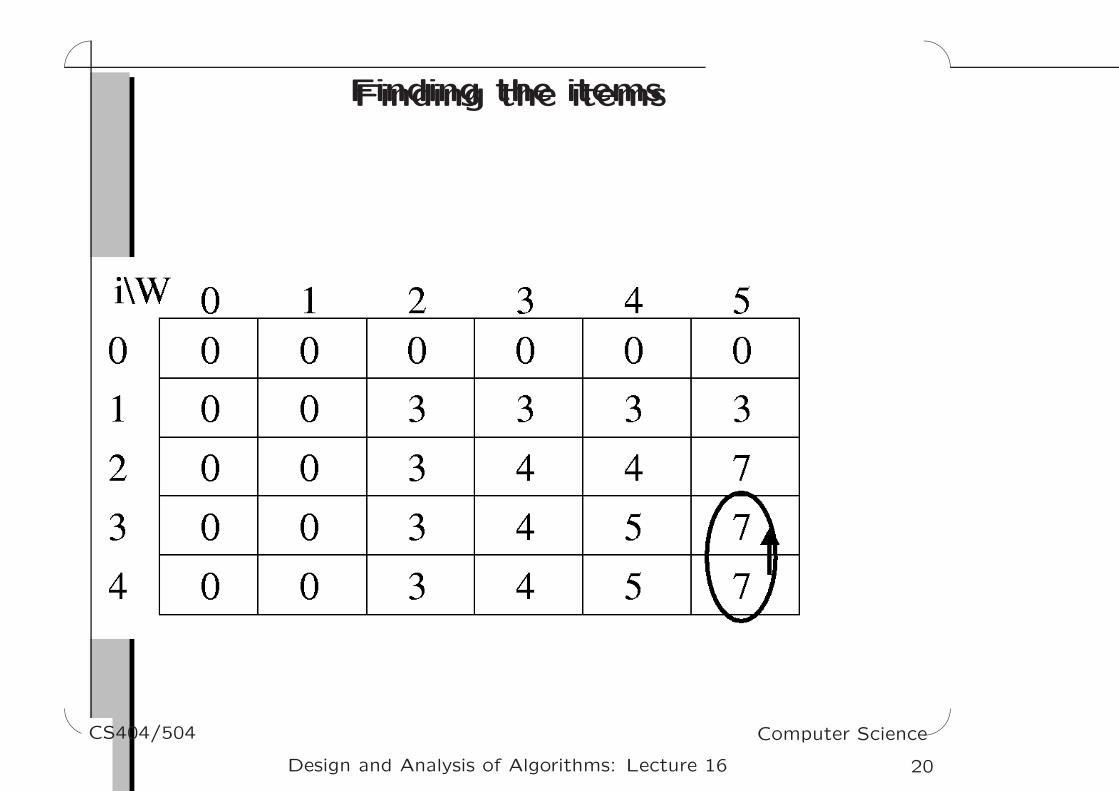
Finding the itemsFinding the items
'
&
$
%CS404/504 Computer Science
20Design and Analysis of Algorithms: Lecture 16
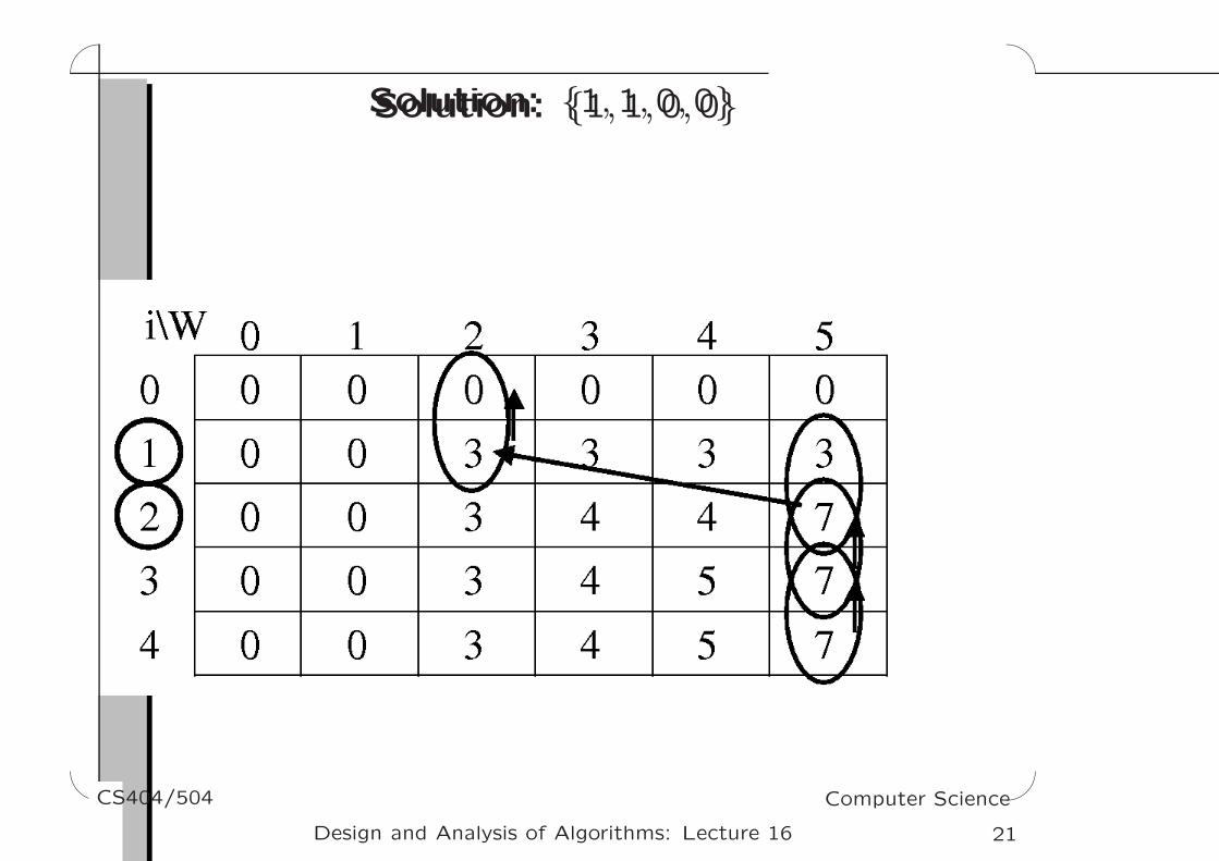
Solution: {1,1,0,0}Solution: {1,1,0,0}
'
&
$
%CS404/504 Computer Science
21Design and Analysis of Algorithms: Lecture 16


