1
The Bioeconomics of Climate Change Adaptation: Coffee Berry Borer and Shade-Grown
Coffee.
Shady S. Atallah
Ph.D. Candidate
Charles H. Dyson School of Applied Economics and Management
Cornell University
438 Warren Hall
Ithaca, NY 14853
E-mail: [email protected]
Miguel I. Gómez
Assistant Professor
Charles H. Dyson School of Applied Economics and Management
Cornell University
321 Warren Hall
Ithaca, NY 14853
E-mail: [email protected]
Selected Paper prepared for presentation at the Agricultural & Applied Economics
Association’s 2014 AAEA Annual Meeting, Minneapolis, MN, July 27-29, 2014.
©Copyright 2014 by Shady S. Atallah and Miguel I. Gómez. All rights reserved. Readers may
make verbatim copies of this document for non-commercial purposes by any means, provided
that this copyright notice appears on all such copies.

2
Bioeconomics of Climate Adaptation: Coffee Berry Borer and Shade-Grown Coffee.
Abstract
Research on climate change in recent decades has disproportionately focused on predicting
impacts while largely ignoring adaptation strategies. How agricultural systems can adapt to
minimize the uncertainty caused by rising temperatures is one of the most important research
issues today. We focus on the coffee berry borer, the most important coffee pest worldwide,
which has recently expanded across the tropics as a result of rising temperatures, threatening
coffee farms worldwide. Intercropping shade trees with coffee trees is being promoted as a
promising climate change adaptation strategy that can protect coffee plantations from micro-
climate variability and reduce pest infestations. Little is known, however, on whether or not the
benefits of the ecological services provided by shade trees justify the ensuing yield reduction
associated with shade-grown coffee production systems. We develop a computational,
bioeconomic model to analyze the ecological and economic sustainability of switching from a
sun-grown to shade-grown coffee system as a climate change adaptation strategy. In particular,
we model the spatial-dynamic pest diffusion at the plant level and evaluate alternative shading
strategies based on farm expected net present values. Using parameters from Colombia,
preliminary model findings suggest that the ecological benefits of shade-grown planting systems
justify the forgone revenues from lower per acre yields only for high levels of shading. We solve
for the threshold net price premium of shade-grown coffee that would make this climate change
adaptation strategy cost-effective at moderate shading levels.
Key words: Bioeconomic Models, Cellular Automata, Colombia, Computational Methods,
Ecological Services, Pest Control, Coffee Berry Borer. JEL Codes: C63, Q54, Q57.

3
Research on climate change in recent decades has disproportionately focused on predicting
impacts of climate change as opposed to examining promising adaptation strategies.
Consequently, very little is known about the benefits and costs of adaptations to climate change
in specific agricultural and agroforestry systems (Antle and Capalbo 2010). For example,
production of coffee, the most valuable tropical export crop worldwide, has been recently
affected by increasing temperatures and consequent damages due to a variety of pests and
diseases (Jaramillo et al. 2011). In particular, the coffee berry borer (CBB), which is the most
damaging coffee pest in all coffee-producing countries, has recently expanded its presence into
higher elevations as a result of rising temperatures across the tropics (Mangina et al. 2010). CBB
damage is likely to worsen over time because of a projected increase in both the number of insect
generations per year and the number of eggs laid per female borer (Jaramillo et al. 2010). The
damage may increase poverty and food insecurity among approximately 120 million people in
South America, East Africa, and Southeast Asia (Vega et al. 2003; Jaramillo et al. 2011). CBB is
likely to be especially severe in Latin America where the pest lacks natural enemies (Avelino,
ten Hoopen and DeClerck 2011). Small-scale, asset-poor coffee producers would be
disproportionately affected because of their limited financial ability to invest in costly adaptation
strategies as well as in more intensive pest and disease management strategies.
Production technologies can be adapted to minimize the uncertainty in coffee production
under rising temperatures in tropical areas. Intercropping shade trees with coffee trees has been
promoted as a rational, economically feasible, and relatively easy-to-implement climate change
adaptation strategy (Lin 2006; Blackman et al. 2008; Jaramillo 2011; Jaramillo et al. 2013).
Shade trees can decrease the temperature around coffee berries by 4 to 5C (Beer et al. 1998;
Jaramillo 2005). Such temperature reduction would imply a drop of 34 percent in the CBB’s
4
intrinsic rate of increase (Jaramillo et al. 2009). Jaramillo et al. (2013) found that CBB
infestation levels in shaded plantations never reached the economic threshold whereas this
threshold was almost always reached in sun-grown plantations. Moreover, coffee berry borer
densities tend to be lower in shaded coffee plantations because of the increased biodiversity and
the ensuing higher populations of natural enemies (Perfecto et al. 2005; Teodoro et al. 2009).
Such pest control ecosystem services have been valued at US $75-310 ha-year -1
in Costa Rica in
terms of avoided damages (Karp et al. 2013). In addition, integrated pest management, which
includes insect trapping, is more successful in shaded than in unshaded coffee plantations
(Dufour et al. 2005). Shade-grown coffee farmers may receive a price premium for their coffee
or direct payments for the by-products and ecosystem services they provide (Somarriba 1992;
Ferraro, Ushida, and Conrad 2005; Kitti et al. 2009; Barham and Weber 2012). Finally, they may
have an additional income through the sale of timber. In the American tropics, laurel (Cordia
alliodora (Ruiz and Pavón) Oken) is a fast-growing, valuable timber species that regenerates
naturally and abundantly in coffee fields and is a source of income for coffee farmers (Mussak
and Laarman 1989; Somarriba 1992; Somarriba et al. 2001). Disentangling the ecological
services and opportunity costs of switching from sun-grown to shade-grown coffee systems
requires careful bioeconomic, spatial-dynamic modeling.
The literature on shade-grown coffee has focused on ecological and agronomic trade-offs
implied by the intercropping of coffee plants with shade plants (Haggar et al. 2011; Jaramillo et
al. 2013). However, we are not aware of research examining the economics of shade-grown
coffee as a climate change adaptation strategy to reduce pest infestations. In particular, it is not
clear whether the expected net economic benefits of switching from sun-grown to shade-grown
coffee systems offset the costs. To fill this gap in the literature, in this paper we develop a

5
bioeconomic model that uses bioeconomic parameters from the CBB literature to simulate pest
diffusion and alternative shading strategies to examine whether and under which conditions the
economic and ecological benefits provided by shade trees justify the ensuing yield reduction
associated with shade-grown production systems.
Literature Review
The unique characteristics of certain pests restrict the choice of modeling approaches of pest
diffusion and control. The first characteristic is that pest infestations are simultaneously driven
by spatial-dynamic biophysical processes. Pest diffusion is affected by the farm’s spatial
configuration, the density and location of individual host and non-host plants (Avelino, ten
Hoopen and DeClerck 2011). In the case of shade coffee, for example, modeling the probability
of infestation for an individual coffee plant would need to be specified, in each time step, as a
function of whether neighboring plants are shade or coffee trees and whether neighboring coffee
trees are infested and at what level. Second, the low-mobility and host-specificity characteristic
of CBB (Avelino, ten Hoopen and DeClerck 2011), and the local effect of a coffee tree’s
microclimate on the reproduction of the CBB (Jaramillo et al. 2009) make it most appropriate to
choose the plant as the modeling unit in a spatial diffusion model. Third, if the goal is to
experiment with alternate coffee farm configurations, where coffee plants are intercropped with
shade plants, a grid-based model is most suitable. Taken together, these three characteristics call
for grid-based, plant-level, spatial-dynamic models of pest diffusion and control.
Spatial Bioeconomic Models
Spatial-dynamic processes have only recently been studied by economists and the
bioeconomic literature on agricultural diseases, pests, and invasive species control is mostly
6
nonspatial thus possibly leading to the recommendation of suboptimal managerial decisions
(Sanchirico and Wilen 1999, 2005; review in Wilen 2007). In most existing spatial models, and
consistently with the application in question, spatial heterogeneity is modeled as exogenous and
fixed over time (e.g., barriers to disease diffusion or constant, location-dependent state-transition
probabilities). In the case of some pests including CBB, however, spatial heterogeneity is neither
exogenous, nor fixed over time. A healthy plant’s probability of being infested is conditional on
the health status of its neighborhood which, in turn, is endogenously determined by the spatial-
dynamic pest diffusion process and the implementation of management strategies. The challenge
of incorporating such spatial feedbacks into state dynamics is a common thread in resource
economics and not confined to pest and disease dynamic models (Smith, Sanchirico and Wilen
2009). Addressing this challenge usually precludes analytical solutions and calls for numerical
methods in most applications.
Cellular Automata
Cellular automata and individual-based models have become the preferred
methodological framework to study socio-ecological complex systems such as diseases and pests
in agro-ecosystems (Grimm and Railsback 2005; Miller and Page 2007). Cellular automata are
dynamic models that operate in discrete space and time on a uniform and regular lattice of cells.
Each cell is in one of a finite number of states that get updated according to mathematical
functions and algorithms that constitute state transition rules. At each time step, a cell computes
its new state given its own old state and the old state of neighboring cells according to transition
rules specified by the modeler (Tesfatsion 2006; Wolfram 1986). The spatial-dynamic structure
is especially relevant when modeling processes that face physical constraints (Gilbert and Terna,
2000) as in the case of pest and disease diffusion in agricultural and agroforestry systems.

7
Although cellular automata models have been extensively employed to model spatial-dynamic
ecological processes including pest diffusion (e.g. BenDor et al. 2006; Prasad et al. 2010), their
use in the agricultural and resource economics literature has been rare (Atallah et al. 2014).
The present work attempts to assess, from a joint economic and ecological standpoint, the
introduction of shade trees in a coffee farm as a response to climate change-driven increased
CBB infestations. We contribute to the bioeconomic and climate adaptation literature by
developing a plant-level model where the effect of climate adaptation measures on pest diffusion
is modeled at the plant level, in a spatial-dynamic way. We formally define the bioeconomic
model, then build the computational model and parameterize it using CBB ecology and coffee
agroforestry literature field data. Using simulation experiments, we generate distributions of
bioeconomic outcomes for the scenario of no infestation, the strategy of no climate change
adaptation (sun-grown system) and five alternative climate change adaptation strategies, namely
five shade-grown systems. We then conduct statistical analyses to rank the expected net present
values generated in each experiment to identify the optimal strategy. Finally, we conduct
sensitivity analyses to key bioeconomic model parameters. We synthesize our modeling process
in Table 1.
[Insert table 1 here]
Bioeconomic Model
The spatial geometry of pest diffusion is represented by a two-dimensional grid representing a
coffee farm. is the set of I x J cells where I and J are the number of rows and columns,
respectively. In our model, there are 1,681 cells ( ) , each being occupied by either a coffee
plant or a shade plant (laurel). Farm rows are oriented north to south with I=41 cells per grid row

8
and J=41 cells per grid column a representing a one-hectare coffee plantation with 1,681 coffee
trees.1
Each cell ( ) has a tree type state , an infestation state , and an age state .
State is a 2 × 1 vector holding a 1 if a cell holds a coffee tree and a zero if the cell holds a
shade tree. State is the infestation state vector of a coffee plant. The vector, of dimension
4×1, holds a 1 for the state that describes a plant’s infection state and zeros for the remaining
three states. A coffee tree can be either Healthy or Infested at a low, moderate, or high level. The
three levels of infestation refer to the percentage of berries in each tree that are infested with
CBB (figure 4, Jaramillo et al. 2013). Given that CBB infestation is host-specific, a shade tree
can only be in the Healthy state (Avelino, ten Hoopen and DeClerck 2011). State is a
9,125×1 vector holding a 1 for a tree’s age in days and a zero for the other ages.
Time progresses in discrete daily steps up to 9,125 days or approximately 25 years. A
coffee plant’s revenue is known to the farmer at time . Yet, the per-plant revenue is random for
periods beyond as it depends on the coffee plant’s infestation state . The revenue from a
cell is a random variable ( ) that depends on the type of tree occupying the cell
( ), its infestation state ( ), and its age ( ). For a cell occupied by a coffee plant, revenue
is equal to ( ) and is function of the infestation state only (equation 0a). Yield
reduction ( ) is equal to 2%, 6%, and 20% when CBB berry infestation is low (10%),
moderate (40%), and high (90%), respectively. A quality penalty ( ) is also imposed on
coffee berries with CBB defects. This penalty is equal to 3%, 23%, and 43% for the three
infestation levels (IL, IM and IH), respectively. The revenue from a cell occupied by a shade plant
is equal to ( ) and is function of the age state only (0b). It is equal to zero until the
shade tree reaches the age of full productivity at which point the cell revenue is equal to the

9
product of the timber yield ( ) and price ( ).2 Symbols, definitions, values, and
references for the parameters are presented in table 2.
(0a) ( ) ( ) (
) ( ) (
)
(0b) ( ) {
[Insert table 2 here]
Given each coffee plant’s state , and an infestation state transition matrix , its
expected infestation state ( ) at time is computed according to the following
infestation-state transition equation:
(1) ( )
where is the expectation operator and is the transpose of matrix . The left-hand side of
equation (1) ( ) is a 4 x 1 vector with a probability of staying in the current infestation
state, a probability of transitioning to the next state, and zeroes elsewhere.
We now describe how the infestation state transition probability matrix P governs the
plant-level CBB diffusion. Coffee plants in state Healthy (H) are susceptible to CBB infestation.
CBB attacks a Healthy coffee plant with a neighborhood-dependent conditional probability b.
Infestation starts at the low level. The transition from state Infested-low to state Infested-
moderate happens with a conditional probability . Similarly, transition from state Infested-
moderate to state Infested-high happens with a conditional probability . Mathematically, P can
be expressed as follows:3
(3) P =
( ) ( )

10
In equation (3), is the Healthy to Infested-low transition probability conditional on
previous own, and neighborhood infestation states and current own, and neighborhood tree type
states. It can be expressed as
(4) ( | )
{
( )
( )
( )
( )
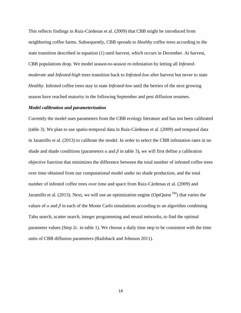
In equation (4), is a state that indicates whether there are any infested coffee plants
and mature shade trees among the eight neighbors of a coffee plant (figure 1). This type of
neighborhood, called Moore neighborhood, is consistent with observed patterns of CBB
diffusion where the pest is shown to spread from tree to tree without any directional preference
(Ruiz-Cárdenas et al. 2009). Consider a healthy coffee plant that is surrounded by healthy coffee
plants with or without shade plants. The probability that it will get infested in the next time step
is equal to zero. If it has at least one infested neighbor, a plant-to-pant infestation occurs with
rate parameter if the coffee tree’s neighborhood does not contain any mature shade tree. That
is, the time a coffee tree with at least one Infested neighbor stays in the Healthy state before
transitioning to the Infested-low state, is an exponentially distributed random variable, with
rate . If a healthy coffee plant has at least one infested neighbor and at least one mature shade
plant in its neighborhood, a plant-to-plant infestation occurs with rate parameter . Given that
shade reduces CBB’s intrinsic rate of increase (Jaramillo et al. 2009), parameter is smaller
than parameter . In each time step (i.e., on any day during the production season), a random
variable determines whether the Healthy to Infested-low state transition happens or not. A
Healthy coffee tree that has one Infested neighbor and no mature shade tree around it is infested

11
by the pest at time t+1 if , where is a random draw from ~ (0, 1).
Conversely, the pest does not colonize the neighboring tree if . When two or more
infestation types are realized (e.g., when a coffee tree has one Infested neighbor to the north and
one Infested neighbor to the southwest), the state transition is determined by the infestation type
that is realized first (Cox 1959).
[Insert figure 1 here]
The probability of transitioning from Infested-low ( ) to Infested-medium ( ) is given
by conditional probability as follows:
(5) ( | ) {
This probability also depends on a coffee plant’s neighborhood state. Coffee trees that
have a mature shade plant in their neighborhood never reach the Infested-medium state (figure 4,
Jaramillo et al. 2013). Those that do not have a mature shade plant in their neighborhood spend a
period in state Infested-low ( ) before they transition to state Infested-moderate ( ). The
waiting time after a coffee tree enters state and before it transitions to state is a random
variable, exponentially distributed with fixed rate parameter .
The Infested-medium ( ) to Infested-high ( ) state transition probability is given by
conditional probability as follows:
(6) ( | ) {
This probability also depends on a coffee plant’s neighborhood state. Coffee trees that
have a mature shade plant in their neighborhood never reach the heavily infested state (figure 4,
Jaramillo et al. 2013). For coffee trees that do not have a mature shade tree in their
neighborhood, the waiting time after they enter state Infested-moderate ( ) and before they

12
transition to state Infested-high ( ) is a random variable, exponentially distributed with fixed
rate parameter . Symbols, definitions, values, and references for the model parameters are
presented in table 3.
[Insert table 3 here]
The objective of a risk-neutral coffee farmer is to maximize the farm’s ENPV by
choosing an optimal shading strategy from a set of strategies, . Each strategy consists of a
share of shade trees in the coffee farm and translates into a binary decision for each cell ( ) at
the beginning of each simulation whereby if a coffee plant is removed and replaced
with a shade plant and 0 otherwise for each ( ) at . Once a coffee plant has been replaced,
it takes the shade tree periods to reach maturity at which point it has an economic value and
provides shade to its neighboring coffee trees thus reducing conditional probabilities , and .
The optimal strategy is therefore the set of cell-level control variables { } that
allocates effort over space so as to yield the maximum ENPV over time. Letting be the
expectation operator over the random cell-level revenues ( ) and the discount
factor 4 at time t (in days) where t {0, 1, 2,…, 9125}, the objective
of a coffee farmer is to
maximize the expected net present value (ENPV) as follows:
(7) ∑ ∑ {
( ∑
) [ ( ) ( )]
( )}
( )
subject to:
(1) ( )
The first expression in the square brackets of equation (7) represents the revenue of a plant in
location( ), which depends on its tree type ( ), infestation ( ) and age ( ) states at
time t. If the farmer has decided to remove a coffee plant in cell ( ) and replace it with a shade
13
plant at t = 0, then is equal to 1 and the revenue from that cell is equal to zero for
periods thus capturing the opportunity cost of having temporarily unproductive shade trees in the
coffee farm. The shade tree revenue is equal to ( ) thereafter, capturing the opportunity
cost of having lower economic value in cells occupied by shade trees as opposed to coffee trees.
If the farmer has left the coffee plant in cell ( ) t = 0, then is equal to 0 and the revenue
from that cell is equal to ( ) minus the unit cost of coffee production . Note that the unit
cost of coffee production depends on the state of its neighborhood : it is lower if there is at
least one mature shade tree in the neighborhood of the coffee tree. This allows the model to be
consistent with experimental findings that per-tree cost of coffee production is lower in shade-
grown systems compared to sun-grown systems, mostly due to fewer fertilizer requirements
(Chamorro, Gallo, and López 1994, table 3).5 Binary variable pre-multiplies two unit costs
associated with shade trees. The first unit cost, is the cost of removing the coffee plant and
planting the shade tree. This cost occurs only at t=0. If a farmer has left cell ( ) occupied with
a coffee plant at t = 0, then is equal to 0, i.e., the farmer does not incur any costs associated
with growing shade trees. The second unit cost, , is the unit production cost of shade trees.
Model Initialization
The beginning of the simulation represents the beginning of a calendar year. Coffee trees are
initialized as Healthy. In September, when berries are ripe, a small percentage (0.5 percent) of
the coffee plants are chosen at random from a uniform spatial distribution (0, ) to
transition from Healthy to Infested-low. This reflects findings in CBB studies indicating that
infested coffee berries from the previous growing season act as a source of re-infestation in the
following season (Jaramillo et. al 2006). In addition, fourteen6 coffee plants situated in the
northwestern border of the farm are chosen at random to transition from Healthy to Infested-low.
14
This reflects findings in Ruiz-Cárdenas et al. (2009) that CBB might be introduced from
neighboring coffee farms. Subsequently, CBB spreads to Healthy coffee trees according to the
state transition described in equation (1) until harvest, which occurs in December. At harvest,
CBB populations drop. We model season-to-season re-infestation by letting all Infested-
moderate and Infested-high trees transition back to Infested-low after harvest but never to state
Healthy. Infested coffee trees stay in state Infested-low until the berries of the next growing
season have reached maturity in the following September and pest diffusion resumes.
Model calibration and parameterization
Currently the model uses parameters from the CBB ecology literature and has not been calibrated
(table 3). We plan to use spatio-temporal data in Ruiz-Cárdenas et al. (2009) and temporal data
in Jaramillo et al. (2013) to calibrate the model. In order to select the CBB infestation rates in no
shade and shade conditions (parameters α and β in table 3), we will first define a calibration
objective function that minimizes the difference between the total number of infested coffee trees
over time obtained from our computational model under no shade production, and the total
number of infested coffee trees over time and space from Ruiz-Cárdenas et al. (2009) and
Jaramillo et al. (2013). Next, we will use an optimization engine (OptQuest TM
) that varies the
values of α and β in each of the Monte Carlo simulations according to an algorithm combining
Tabu search, scatter search, integer programming and neural networks, to find the optimal
parameter values (Step 2c. in table 1). We choose a daily time step to be consistent with the time
units of CBB diffusion parameters (Railsback and Johnson 2011).

15
Experimental Design
We design and implement Monte Carlo experiments to evaluate a discrete set of shading
strategies by comparing their bioeconomic outcomes to those resulting from a strategy of no
shade. Each experiment consists of a set of 300 simulation runs, over 9,125 days (25 years), on a
coffee farm of 1,681 coffee trees. Experiments differ in the fraction of shade trees to total
number of trees in the coffee farm. We experiment with shading strategies that have a fraction of
shade trees below and above the 5-6% fraction (70 shade trees/acre approximately) required for
shade-grown coffee certifications (SAN 2010). We consider the following shading strategies: 0
(sun-grown), 2, 4, 6, 8, and 10% shading levels.
Survey data indicate that, in most cases, timber shade trees are recruited from the
naturally occurring regeneration (Somarriba 1992 and references therein); we therefore assign
the location of shade trees using random draws from a uniform distribution.
Outcome realizations for a run within an experiment differ due to random spatial
initialization of the infestation and the shading strategies and due to subsequent random spatial
pest diffusion. Data collected over simulation runs are the expected values of the bioeconomic
outcomes under each strategy (Step 3, table 1): expected net present values and average CBB
prevalence. In order to find the optimal shading strategy, we employ the objective function
(equation 7) to rank the coffee farm net values under the alternative strategies. Finally, we
conduct statistical tests to rank the shading strategies and find the optimal strategy (Step 4, table
1). The model is written in Java and simulated using the software AnyLogicTM
(XJ
Technologies).
Preliminary Results

16
Our preliminary simulation results indicate that transitioning from a sun-grown system to a
shade-grown system as a climate adaptation strategy to increased CBB infestations is not ENPV-
improving at the 5-6% recommended shading levels. That is, the baseline scenario of no shade
trees yields a higher ENPV than any of the scenarios that include shade trees at any of the
shading levels ranging between 2 and 10% (table 4). Under the baseline scenario of no shade, the
average prevalence of highly infested coffee trees is equal to 13.8% and the ENPV over 2 years
is $17.028 thousand per hectare. Intercropping coffee plants with shade trees reduces CBB
prevalence by 2-8% but it also reduces the ENPV by 12-33% for the shading levels between 2
and 10%, respectively (table 4). In the shading interval considered, the benefits of reduced CBB
incidence accruing to shade trees appear to be offset by the lower farm yields resulting from
having smaller per-tree yields and fewer coffee trees per hectare.
[Insert table 4 here]
We conduct additional simulations to (1) examine the relationship between increased
shading and CBB control; and (2) find the threshold shading level beyond which switching from
a sun-grown to a shade-grown system is ENPV-improving. We find that the pest control services
provided by shade trees increase at decreasing rates with the shading level (figure 2). Our results
indicate that, under baseline model parameters, a farmer would need to achieve a shading level
of 16% for the shade pest control benefits to justify the opportunity costs and direct costs of
transitioning from a high-yield sun-grown system to a lower-yield shade-grown system (figure
3).
[Insert figure 2 here]
[Insert figure 3 here]

17
The baseline model does not account for the price premium or transfer shade coffee
farmers may receive as a payment for ecosystem protection (Ferraro et al. 2005). We investigate
how the optimal shading level changes if there is a price premium paid to shade-grown coffee
farmers. We consider a price premium of $0.44/Kg, the half of which covers the costs of
certification. We find that the ENPVs for the 10, 12, and 15% shading levels are $16.613,
$17.366, and $18.487 per hectare, respectively. That is, the threshold shading level decreases
from 16% (no price premium) to 12% under a net price premium of $0.22/Kg.
Whether higher shading levels are feasible from an agronomic standpoint depends on the
particular shade tree species. For instance, in Colombia, shading levels are between 6 and 12%
(100-200 trees per hectare) (Liegel and Stead 1990). If the threshold shading level is not feasible
due to tree species-specific agronomic constraints (e.g., size of tree canopy), then it might be that
the economically optimal shading strategies cannot be achieved. Alternatively, higher net price
premiums might be needed to make the transition economically justified for recommended shade
levels of 6%. For instance, we find that the net price premium would need to be more than twice
as large for the 6% shading level ($0.44/Kg) to yield ENPVs higher than those of a sun-grown
strategy (the ENPV of a 6% shading strategy is equal to $16.784 per hectare for a net price
premium of $0.44/Kg).
Concluding Remarks and Next Steps
This paper offers a bioeconomic framework to analyze the biological and economic
sustainability of planting shade trees as a climate change adaptation strategy in coffee farms. We
apply the model to the coffee berry borer (CBB) diffusion under alternative shading strategies
and find that shading would need to be higher than currently recommended for the pest control

18
benefits of shade to justify the costs of switching from a sun-grown to a shade system.
Alternatively, coffee certification costs would need to be almost inexistent for shade-grown
coffee price premiums to offset the direct and opportunity costs of transitioning from sun-grown
to shade-grown systems as an adaptation to climate change. In reality, certification can be
prohibitively expensive for developing country growers especially for groups of less than 10,000
coffee farmers (Gómez et al. 2011).
Future research should model the infestation probabilities explicitly as a function of
temperature. Such exercise is particularly important to identify the IPCC climate change
scenarios for which shading strategies are economically justified. The model can also be
extended to incorporate spatial-dynamic pest externalities caused by the flow of CBB from
neighboring coffee farms with higher CBB prevalence and lower shading levels. In such
situations, shading strategies might need to allow shade tree intercropping to be spatially
nonrandom. For example, alternative strategies can allow the density of shade trees to be higher
at the border of coffee farms serving as the initial point of entry of CBB.

19
References
Antle, J. M., and S. M. Capalbo. 2010. Adaptation of agricultural and food systems to climate
change: an economic and policy perspective. Applied Economic Perspectives and
Policy, 32 (3), 386-416.
Avelino, J., ten Hoopen, G. M., and DeClerck, F. 2011. Ecological mechanisms for pest and
disease control in coffee and cacao agroecosystems of the neotropics. In Ecosystem
Services from Agriculture and Agroforestry, ed. Rapidel et al., 91-118. London: Earthscan.
Barham, B. L., and Weber, J. G. 2012. The economic sustainability of certified coffee: Recent
evidence from Mexico and Peru. World Development, 40(6), 1269-1279.
Beer, J., Muschler, R., Kass, D., and E. Somarriba. 1998. Shade management in coffee and cacao
plantations. Agroforestry Systems 38: 139–164
BenDor, T. K., Metcalf, S. S., Fontenot, L. E., Sangunett, B., and Hannon, B. 2006. Modeling
the spread of the emerald ash borer. Ecological modelling,197 (1), 221-236.
Blackman, A., Albers, H. J., Avalos-Sartorio, B., and Murphy, L. C. 2008. Land cover in
managed forest ecosystem: Mexican shade coffee. American Journal of Agricultural
Economics, 90(1), 216–231
Chamorro G., Gallo A. and Lopez R. 1994. Evaluación económica del sistema
agroforestal café asociado con nogal. Cenicafé 45(4): 164–170
Cox, D. R. 1959. The Analysis of Exponentially Distributed Life-Times with Two Types of
Failure. Journal of the Royal Statistical Society. Series B 21: 411-421.
Dufour B.P., González M.O., Mauricio J.J., Chávez B.A., and Ramírez Amador R. 2005.
Validation of coffee berry borer (CBB) trapping with the BROCAP® trap. In: XX

20
International Conference on Coffee Science, 11-15 October 2004, Bangalore, India. ASIC,
Paris, France, 1243-1247.
Ferraro, P. J., Uchida, T., and Conrad, J. M. 2005. Price premiums for eco-friendly commodities:
are ‘green’markets the best way to protect endangered ecosystems? Environmental and
Resource Economics, 32(3), 419-438.
Gilbert, N. and P. Terna. 2000. How to Build and Use Agent-Based Models in Social Science.
Mind and Society 1: 57-72.
Gómez, M. I., Barrett, C. B., Buck, L. E., De Groote, H., Ferris, S., Gao, H. O., ... and Yang, R.
Y. 2011. Research principles for developing country food value cains. Science, 332 (6034),
1154-1155.
Grimm, V., and Railsback, S. F. 2005. Individual-based modeling and ecology. Princeton
university press.
Haggar, J., Barrios, M., Bolaños, M., Merlo, M., Moraga, P., Munguia, R., and de MF Virginio,
E. 2011. Coffee agroecosystem performance under full sun, shade, conventional and
organic management regimes in Central America. Agroforestry systems, 82 (3), 285-301.
Jaramillo A. 2005. Andean climate and coffee in Colombia. Colombian National Federation of
Coffee Growers. Centro Nacional de Investigaciones de Cafe´– Cenicafe´. Chinchina,
Colombia. 192p. (in Spanish).
Jaramillo, J., C. Borgemeister, and P. Baker. 2006. “Coffee berry borer Hypothenemus hampei
(Coleoptera: Curculionidae): searching for sustainable control strategies.” Bulletin of
Entomological Research 96 (3): 223-233.

21
Jaramillo J, Chabi-Olaye A, Kamonjo C, Jaramillo A, Vega FE, et al. 2009. Thermal Tolerance
of the Coffee Berry Borer Hypothenemus hampei: Predictions of Climate Change Impact
on a Tropical Insect Pest. PLoS ONE 4(8).
Jaramillo, J., Chabi-Olaye, A., and Borgemeister, C. 2010. Temperature-dependent development
and emergence pattern of Hypothenemus hampei (Coleoptera: Curculionidae: Scolytinae)
from coffee berries” Journal of Economic Entomology, 103(4), 1159-1165.
Jaramillo, J., Muchugu, E., Vega, F. E., Davis, A., Borgemeister, C., and Chabi-Olaye, A. 2011.
Some like it hot: the influence and implications of climate change on coffee berry borer
(Hypothenemus hampei) and coffee production in East Africa. PLoS One, 6(9), e24528.
Jaramillo, J., Setamou, M., Muchugu, E., Chabi-Olaye, A., Jaramillo, A., Mukabana, J.,and
Borgemeister, C. 2013. Climate Change or Urbanization? Impacts on a Traditional Coffee
Production System in East Africa over the Last 80 Years. PloS one, 8(1), e51815.
Johnson, M. D., Kellermann, J. L., and Stercho, A. M. 2010. Pest reduction services by birds in
shade and sun coffee in Jamaica. Animal conservation, 13(2), 140-147.
Karp, D. S., Mendenhall, C. D., Sandí, R. F., Chaumont, N., Ehrlich, P. R., Hadly, E. A., and
Daily, G. C. 2013. Forest bolsters bird abundance, pest control and coffee yield. Ecology
letters, 16 (11), 1339-1347.
Kitti, M., Heikkila, J., and Huhtala, A. 2009. ‘Fair’ policies for the coffee trade—Protecting
people or biodiversity? Environment and Development Economics, 14(6), 739–758
Liegel, L.H., and J.W. Stead. 1990. Cordia alliodora (Ruiz and Pav.) Oken: laurel, capá prieto.
In R.M. Burns and B.H. Honkala (Techn. Coords.). Silvics of North America, volume 2,
Agricultural Handbook 654, pp. 270-277. U.S. Department of Agriculture, Washington,

22
D.C. Available at
http://www.na.fs.fed.us/pubs/silvics_manual/volume_2/cordia/alliodora.htm. Last accessed
7/14/2014.
Lin, B. B. 2007. “Agroforestry management as an adaptive strategy against potential
microclimate extremes in coffee agriculture.” Agricultural and Forest
Meteorology, 144(1), 85-94.
Mangina FL, Makundi RH, Maerere AP, Maro GP, and Teri JM. 2010. “Temporal variations in
the abundance of three important insect pests of coffee in Kilimanjaro region, Tanzania.”
In: 23rd International Conference on Coffee Science. Bali, Indonesia 3–8 October 2010.
ASIC, Paris
Miller, J. H. and S. E. Page, .2007. “Complex Adaptive Systems: An Introduction to
Computational Models of Social Life.” Princeton University Press, Princeton, USA, 284
pp.
Mussak, M. F., and Laarman, J. G. 1989. Farmers' production of timber trees in the cacao-coffee
region of coastal Ecuador. Agroforestry systems, 9 (2), 155-170.
Perfecto, I., Vandermeer, J., Mas, A., and Pinto, L. S. 2005. Biodiversity, yield, and shade coffee
certification. Ecological Economics, 54(4), 435-446.
Prasad, A. M., Iverson, L. R., Peters, M. P., Bossenbroek, J. M., Matthews, S. N., Sydnor, T. D.,
and Schwartz, M. W. 2010. Modeling the invasive emerald ash borer risk of spread using a
spatially explicit cellular model. Landscape ecology, 25(3), 353-369.
Ruiz-Cárdenas, R., Assunção, R. M., & Demétrio, C. G. B. (2009). Spatio-temporal modelling of
coffee berry borer infestation patterns accounting for inflation of zeroes and missing
values. Scientia Agricola, 66(1), 100-109.

23
Sanchirico, J. and J. Wilen. 1999. “Bioeconomics of Spatial Exploitation in a Patchy
Environment.” Journal of Environmental Economics and Management 37: 129-150.
–––. 2005. “Optimal Spatial Management of Renewable Resources: Matching Policy Scope to
Ecosystem Scale.” Journal of Environmental Economics and Management 50: 23–46.
Smith, M. D., J. N. Sanchirico, and J. E. Wilen. 2009. “The Economics of Spatial-Dynamic
Processes: Applications to Renewable Resources.” Journal of Environmental Economics
and Management 57: 104-121.
Somarriba, E. 1992. “Timber harvest, damage to crop plants and yield reduction in two Costa
Rican coffee plantations with Cordia alliodora shade trees.” Agroforestry systems 18, no.
1: 69-82.
Sustainable Agriculture Network. 2010. Sustainable Agriculture Standard. Available at
http://sanstandards.org/userfiles/SAN-S-1-
1_2%20Sustainable%20Agriculture%20Standard_docx(1).pdf. Last accessed 7/24/2014
Teodoro A, Klein AM, Reis PR, and Tscharntke T. 2009. “Agroforestry management affects
coffee pests contingent on season and developmental stage.” Agricultural and Forest
Entomology 11: 295–300.
Tesfatsion, L., and K. L. Judd (ed.). 2006. Handbook of Computational Economics, Elsevier,
edition 1, volume 2, number 2.
United States Department of Agriculture Foreign Agricultural Service 2014. “Colombia Coffee
Annual Subsidies Subside as Prices Climb and Production Recovers”, GAIN report,
available at http://gain.fas.usda.gov/, last accessed 7/21/2014.
Vega, F.E., Rosenquist, E., and Collins, W. 2003. “Global project needed to tackle coffee
crisis.” Nature 425 (6956), 343.

24
Wilen, J. 2007. “Economics of Spatial–Dynamic Processes.” American Journal of Agricultural
Economics 89: 1134–1144.
Wolfram, S. (ed.). 1986. “Theory and Applications of Cellular Automata.” World Scientific,
Singapore.

25
Table 1. Overview of the modeling process
Modeling Step Tool
1. Formal model.
Define bioeconomic model. None.
2. Computational model.
2a. Model specification.
- Specify cellular automata model by defining:
o Space and time
o States and state transitions
- Define model parameters and variables.
Java,
AnyLogic.
2b. Model verification.
- Conduct simulation and collect simulated data.
- Debug to ensure consistency in model behavior between computational model
and formal model.
Java,
AnyLogic.
2c. Model calibration
Define optimization experiment that aims to find the ‘optimal’ CBB diffusion
values using field data from the literature.
OptQuest,
AnyLogic.
2d. Model validation
Validate calibrated model by testing that the average CBB prevalence levels
under sun vs. under shade fall within intervals reported in the literature.
Java,
AnyLogic.
3. Simulation experiments
Define and conduct Monte Carlo experiments: scenarios of ‘no shade’, and
multiple shading strategies.
Java,
AnyLogic.
4. Statistical analyses
Conduct statistical tests on the differences between expected net present values. Stata.
5. Sensitivity analyses
Repeat steps 3 and 4 for each parameter considered in the sensitivity analysis.

26
Table 2. Coffee tree yield and quality reduction parameters
Infestation state ( ) Berry infestation
level (%)
Yield
reduction (%)a
Quality penalty (%) b
H <1 0 0
IL 1-10 2 3
IM 10-25 6 23
IH >25 20 43
a Duque and Baker (2003
b National Coffee Federation in Colombia, Price list, May 13 2013.

27
Table 3. CBB diffusion parameters
Parameter Description Value Unit Sources
α Exponential probability rate
parameter, no shade.
0.0100 day -1
Preliminary model
calibration.
Assumed.
β Exponential probability rate
parameter, shade.
0.0005 day -1
Average waiting time between
and state, no shade.
15 days Johnson et al. (2009).
Average waiting time between
and state, no shade.
120 days Johnson et al. (2009) and
Ruiz-Cardenas et al. (2009).

28
Table 3.2 Sun-grown and shade-grown coffee production parameters
Coffee production system
Sun Shade
Parameter Description Unit Valuea Value
a
Coffee
( ) Yield Kg/tree/yearb 0.82 0.61
( ) Pricec USD/kg 3.16 3.16
Production costd USD/tree/year
b 1.28 1.12
Coffee removal costd,e USD/tree n/a 0.12
Timber
Yield inches/tree/yearb n/a 0.0099295
Priced USD/inch n/a 537
Production costd USD/ tree n/a 0
Discount factor day -1
0.9997f 0.9997f
n/a is not applicable a Parameter values are from
Chamorro, Gallo and López (1994), unless otherwise noted.
b Note that these values are expressed in per-day terms in the model.
c National Coffee Federation in Colombia, Price list, May 13 2013
d Values are expressed in real terms. e Duque and Baker (2003).
f Equivalent to an annual discount rate of 10%.

29
Table 4. Coffee shading strategies: effect on coffee berry borer (CBB) control and
expected net present values (ENPV)
Shading
strategy (%
shade plants)
CBB prevalence
(%)a
Change in
CBB
prevalence b
ENPV c
(1,000$/ha)
Percent
change in
ENPV d
0 (sun-grown) 13.8 (10) n/a 17.028 (0.05) n/a
2 11.4 (8) -2.4 11.455 (0.04) -33
4 9.4 (6) -4.5 12.375 (0.03) -27
6 6.5 (5) -6.0 13.236 (0.03) -22
8 7.4 (4) -7.4 14.084 (0.03) -17
10 5.4 (3) -8.4 14.904 (0.03) -12
n/a is not applicable a Average
CBB
prevalence over growing seasons= number of highly infested coffee plants
divided by the total number of coffee plants b
Change in CBB prevalence=prevalence (Strategy)-prevalence (0% shading) c Expectations are obtained from 300 simulations
d Percent change in ENPV=[ENPV (Strategy)-ENPV (0% shading)]/ ENPV (0% shading)
e Standard deviations in parentheses
30
Figure 1. Neighborhood of a coffee plant (i, j)
i-1, j-1 i-1,j i+1,j +1
i,j-1 i, j i, j+1
i+1, j-1 i+1, j i+1, j+1

31
Figure 2. Production of pest control at increasing shading levels
0%
2%
4%
6%
8%
10%
12%
2 4 6 8 10 12 14 16 18 20
Per
cen
tage
po
int
red
uct
ion
in C
BB
in
fest
atio
n
Shading level (% shade)

32
Figure 3. Effect of shading on expected net present values
10
11
12
13
14
15
16
17
18
19
0 2 4 6 8 10 12 14 16 18 20
Exp
ecte
d N
et P
rese
nt
Val
ues
(1
,00
0 $
/hec
tare
)
Shading strategies (% shade)
Shade
No shade

33
Endnotes
1 Approximately 95 percent of Colombia’s coffee smallholders farm on less than 5 hectares of
land (USDA FAS 2014).
2 Note that, among the many outputs and uses of laurel, we only consider timber in this article.
The tree is also grown for fruits, honey production, and ethanol production among other uses
(Liegel and Stead 1990).
3P reads from row (states H, IL, IM, and IH at time t) to column (states H, IL, IM, and IH at time
t+1).
4
( ) , where is the discount rate.
5 Shade trees improve soil fertility by recycling nutrients which are not accessible to coffee trees
and by increasing in the soil organic matter from leaf fall, among other mechanisms (Beer 1987).
6 This number is chosen so as to reproduce the proportion of border coffee plants in the
northwestern corner of the coffee farm that received the infestation from a neighboring farm in
Ruiz-Cárdenas et al. (2009).


