
The challenge of Galaxy modelling
James Binney
Oxford University
Outline
• The why & how of modelling the Galaxy
• The why & how of using actions
• Simple DFs for the disc(s)
• Determining the solar motion
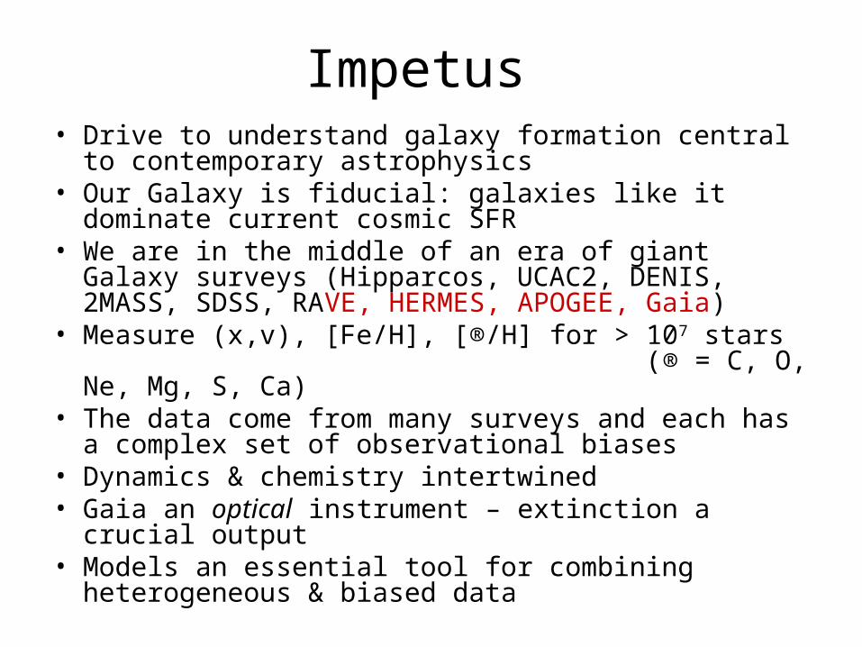
Impetus • Drive to understand galaxy formation central to
contemporary astrophysics• Our Galaxy is fiducial: galaxies like it dominate current
cosmic SFR• We are in the middle of an era of giant Galaxy surveys
(Hipparcos, UCAC2, DENIS, 2MASS, SDSS, RAVE, HERMES, APOGEE, Gaia)
• Measure (x,v), [Fe/H], [®/H] for > 107 stars (® = C, O, Ne, Mg, S, Ca)
• The data come from many surveys and each has a complex set of observational biases
• Dynamics & chemistry intertwined • Gaia an optical instrument – extinction a crucial output• Models an essential tool for combining heterogeneous &
biased data

Key questions
• How violent is our history?– Mergers vs accretion– Relation to WHIM (>50% of baryons)
• Can we identify relics?– By groupings in chemistry & orbit space
• What did the Local Group look like at z?– Vital for interpretation of high-z obs
• When did bar form?– Has it been renewed? – Impact on DM? – Role in secular heating?
• What is the structure of the ISM?– Extinction, exchange of matter with WHIM

Hierarchical modelling
• MW complex system, data heterogeneous & rich• Multi-stage modelling essential• Require models that can be
– Evaluated in different ©s– Viewed at varying resolution
• solar nhd, far MW• with & without chemistry
– Capable of refinement– Provide understanding
• perturbation theory
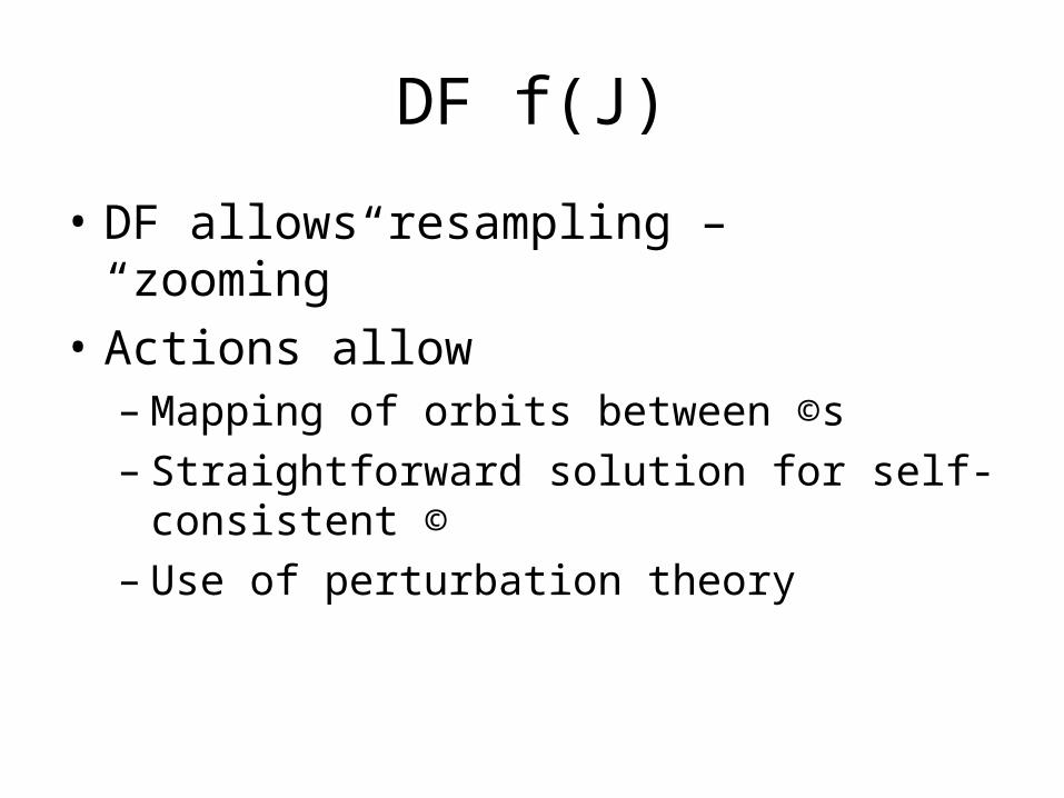
DF f(J)
• DF allows resampling – “zooming”
• Actions allow – Mapping of orbits between ©s– Straightforward solution for self-consistent ©– Use of perturbation theory
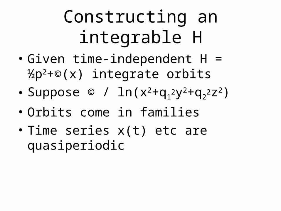
Constructing an integrable H
• Given time-independent H = ½p2+©(x) integrate orbits
• Suppose © / ln(x2+q12y2+q2
2z2)
• Orbits come in families
• Time series x(t) etc are quasiperiodic
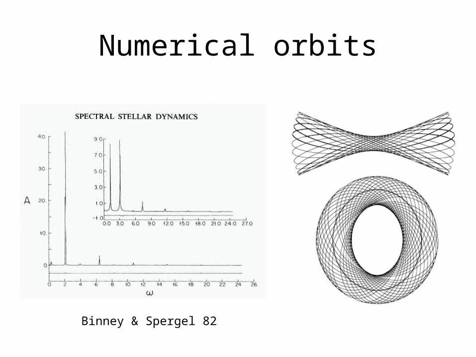
Numerical orbits
Binney & Spergel 82

Angles & actions
• Quasiperiodic orbits ) exist integrals J1, J2, J3 that can be complemented by coordinates µ1, µ2, µ3 with trivial eqns of motion Ji = constat and µi = it + const
• Orbits 3-tori labelled by J with µ defining position on torus
• Torus null in sense storusdx¢ dv = 0• Question is: how to find (x, v)(J,µ) for
given ©?

Analytic models(de Zeeuw MNRAS 1985)
• Most general: – Staeckel © defined in terms of confocal
ellipsoidal coordinates
• © separable in x,y,z and ©(r) limiting cases
• Staeckel © yields analytic Ii but numerical integration required for Ji,µi
• Everything analytic for 3d harmonic oscillator and isochrone

Torus programme
• Map toy torus from harmonic oscillator or isochrone into target phase space
• Use canonical mapping, so image is also null
• Adjust mapping so H = const on image

e.g. Box orbits (Kaasalainen & Binney 1994)
• Orbits » bounded by confocal ellipsoidal coords (u,v)
• x’= sinh(u) cos(v); y’= cosh(u) sin(v)
• When (u,v) cover rectangle, (x’,y’) cover realistic box orbit
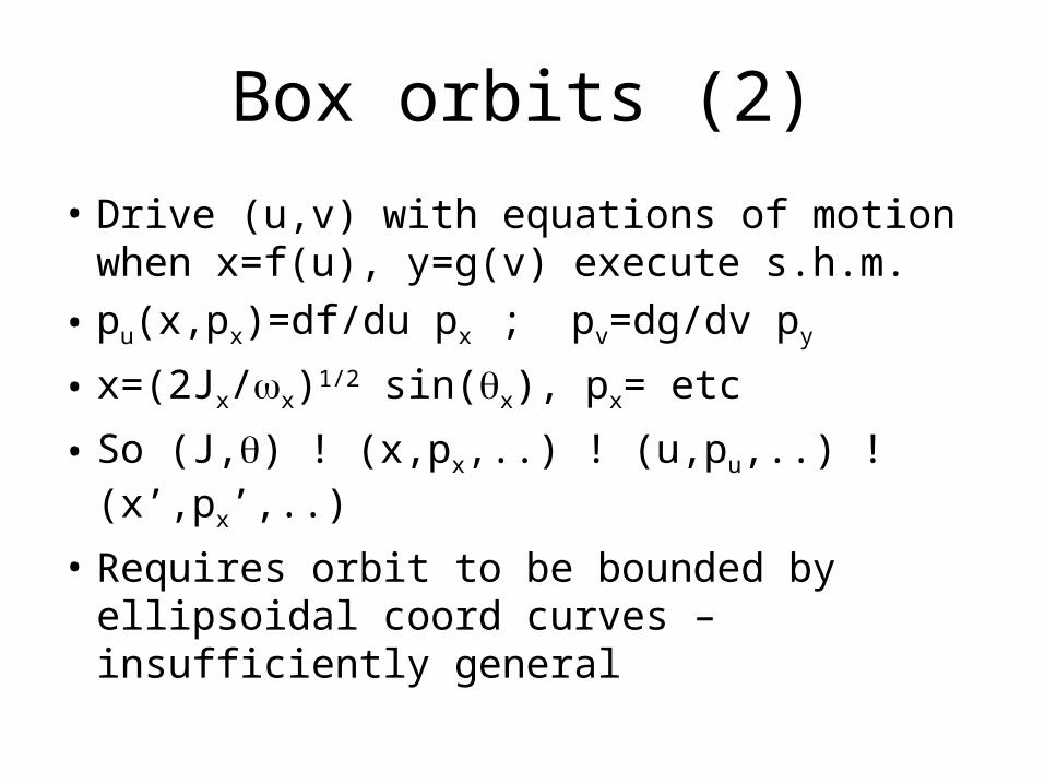
Box orbits (2)
• Drive (u,v) with equations of motion when x=f(u), y=g(v) execute s.h.m.
• pu(x,px)=df/du px ; pv=dg/dv py
• x=(2Jx/x)1/2 sin(x), px= etc
• So (J,) ! (x,px,..) ! (u,pu,..) ! (x’,px’,..)
• Requires orbit to be bounded by ellipsoidal coord curves – insufficiently general
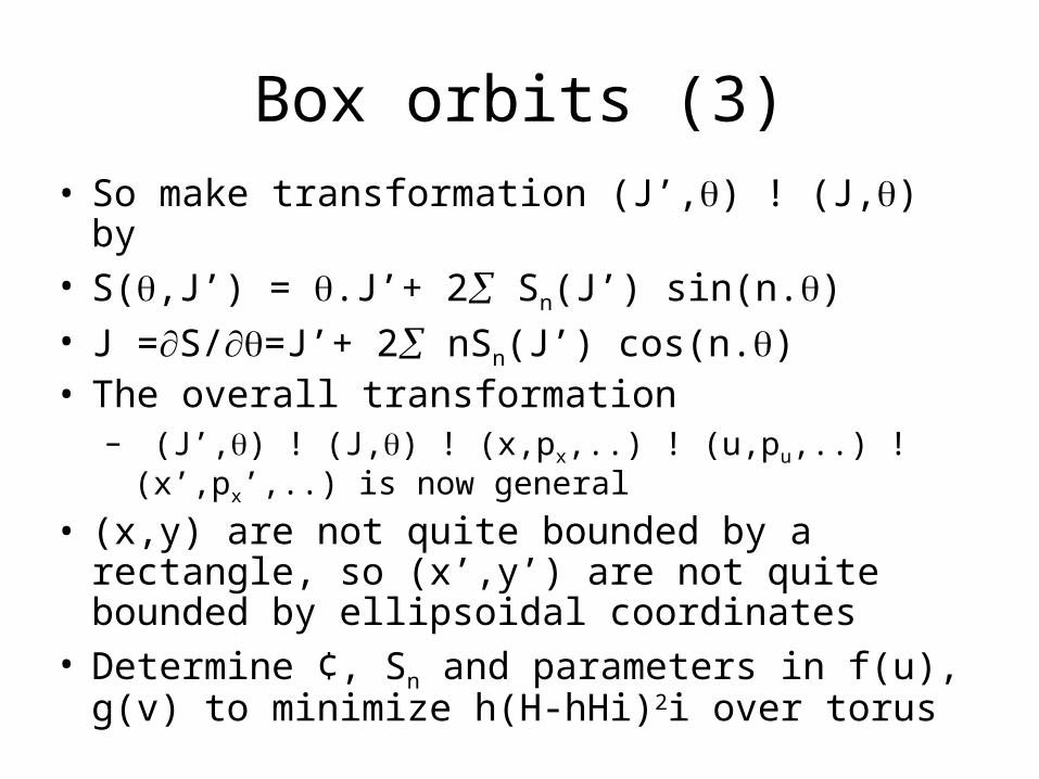
Box orbits (3)• So make transformation (J’,) ! (J,) by• S(,J’) = .J’+ 2 Sn(J’) sin(n.)• J =S/=J’+ 2 nSn(J’) cos(n.)• The overall transformation
– (J’,) ! (J,) ! (x,px,..) ! (u,pu,..) ! (x’,px’,..) is now general
• (x,y) are not quite bounded by a rectangle, so (x’,y’) are not quite bounded by ellipsoidal coordinates
• Determine ¢, Sn and parameters in f(u), g(v) to minimize h(H-hHi)2i over torus
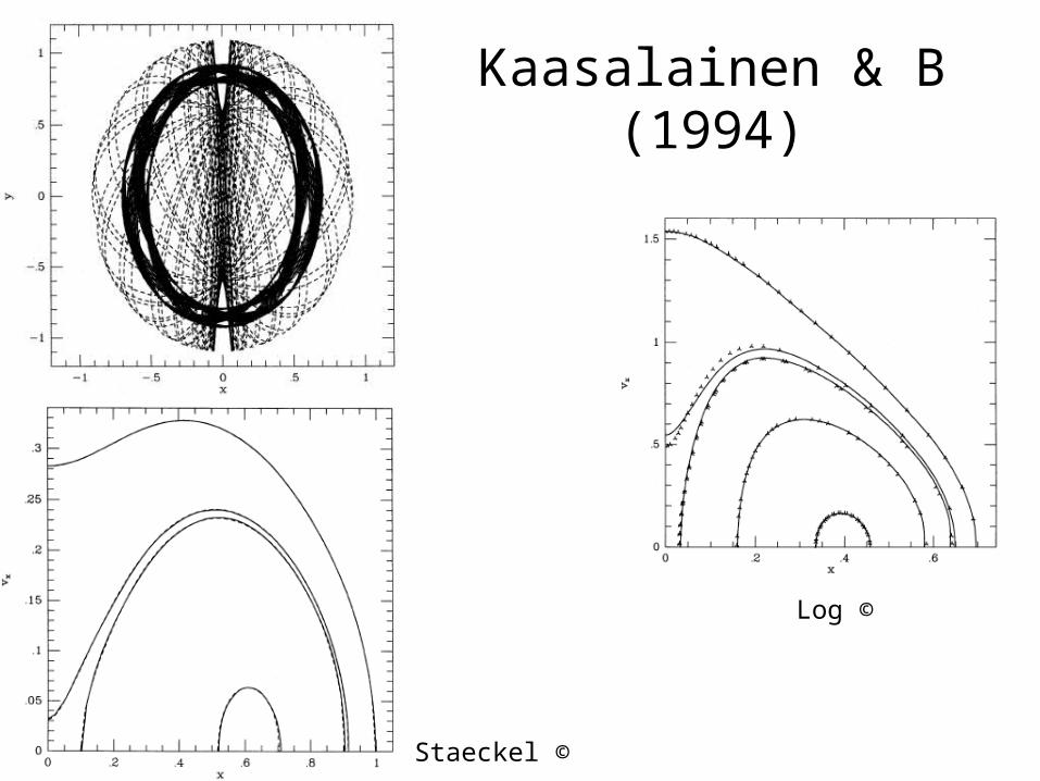
Kaasalainen & B (1994)
Log ©
Staeckel ©
(J 0r ;µ
0r ; ::)
S=J µ0+¢¢¢
!(J r ;µr ; ::)
Isochr
!(pr ;r; ::)
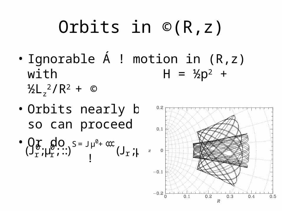
Orbits in ©(R,z)
• Ignorable Á ! motion in (R,z) with H = ½p2 + ½Lz
2/R2 + ©
• Orbits nearly bounded by (u,v) so can proceed as above
• Or do

General ©(x,y,z)
• No significant modifications required for general © (including rotating frame of reference; Kaasalainen 1995)
What have we achieved?• Analytic formulae x(J,µ) and v(J,µ)• So can find at what µ star is at given x & get corresponding v• If orbit integrated in t, star will just come close, & we have to
search for closest x• Orbit characterized by actions J
– essentially unique unlike initial conditions
• Sampling density apparent because d6w=(2¼)3d3J• The J are adiabatic invariants – useful when © slowly
evolving– mass-loss, 2-body relax, disc accretion…

What have we achieved (2)• Real-space characteristics of orbits naturally related to J so can design
DF f(J) to give component of specified shape & kinematics (GDII sec 4.6)
• Numerically orbit given by parameters of toy plus point transformations plus <~100 Sn (cf 1000s of (x,p)t if orbit integrated in t)
• Sn are continuous fns of J, so we can interpolate between orbits• The likelihood of arbitrary data given a model can be calculated by
doing 1-d integral for each star • Given f(J) have a stable scheme for determining self-consistent ©• Fokker-Planck eqn exceptionally simple in a-a coordinates• We are equipped to do Hamiltonian perturbation theory
Choice of DF
• Represent DF with analytic f(J) – To give physical insight– To keep DF smooth
• low entropy null hypothesis
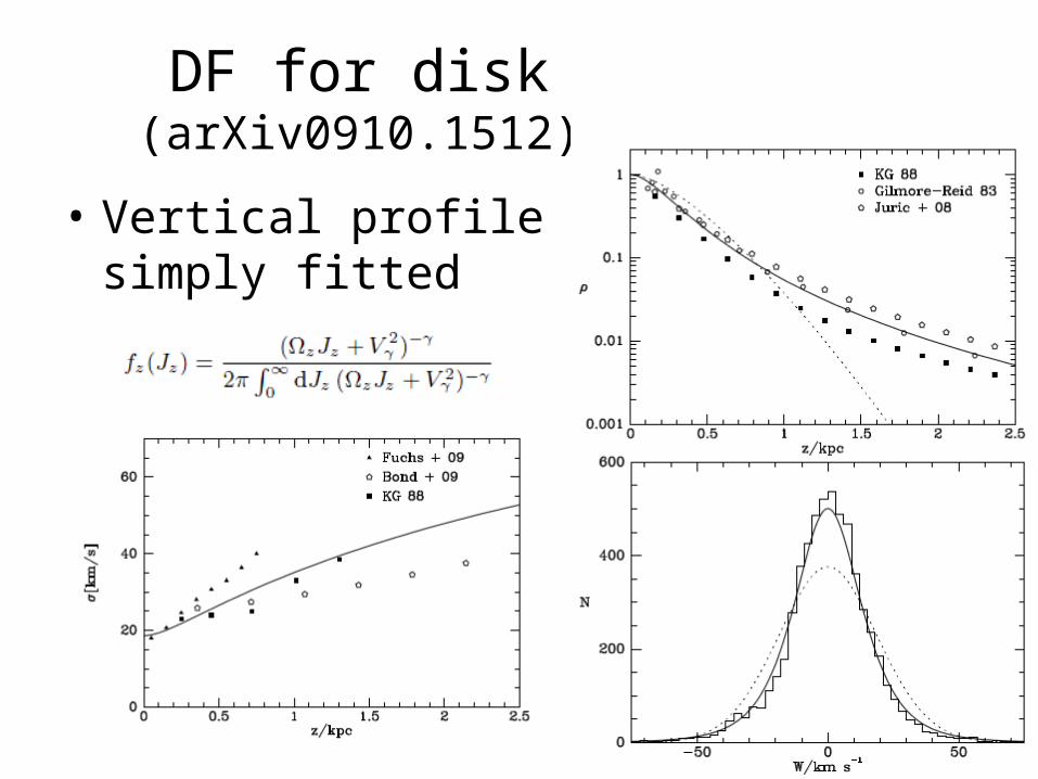
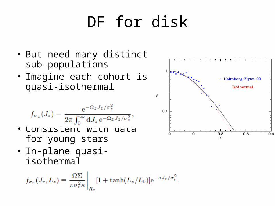
DF for disk(arXiv0910.1512)
• Vertical profile simply fitted
DF for disk
• But need many distinct sub-populations
• Imagine each cohort is quasi-isothermal
• Consistent with data for young stars
• In-plane quasi-isothermal
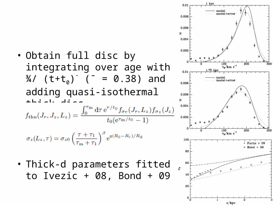
• Obtain full disc by integrating over age with ¾/ (t+t0)¯ (¯ = 0.38) and adding quasi-isothermal thick-disc
• Thick-d parameters fitted to Ivezic + 08, Bond + 09
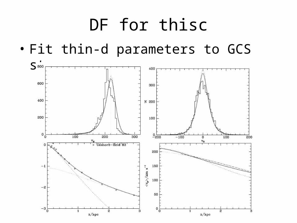
DF for thisc• Fit thin-d parameters to GCS stars
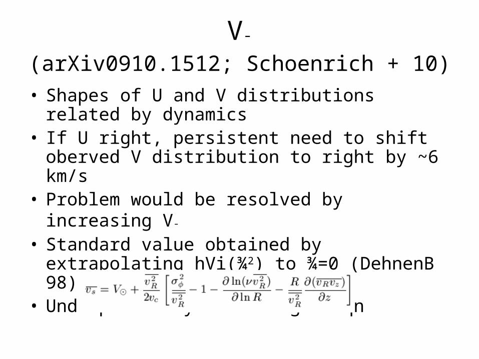
V¯
(arXiv0910.1512; Schoenrich + 10)
• Shapes of U and V distributions related by dynamics
• If U right, persistent need to shift oberved V distribution to right by ~6 km/s
• Problem would be resolved by increasing V¯
• Standard value obtained by extrapolating hVi(¾2) to ¾=0 (DehnenB 98)
• Underpinned by Stromberg’s eqn
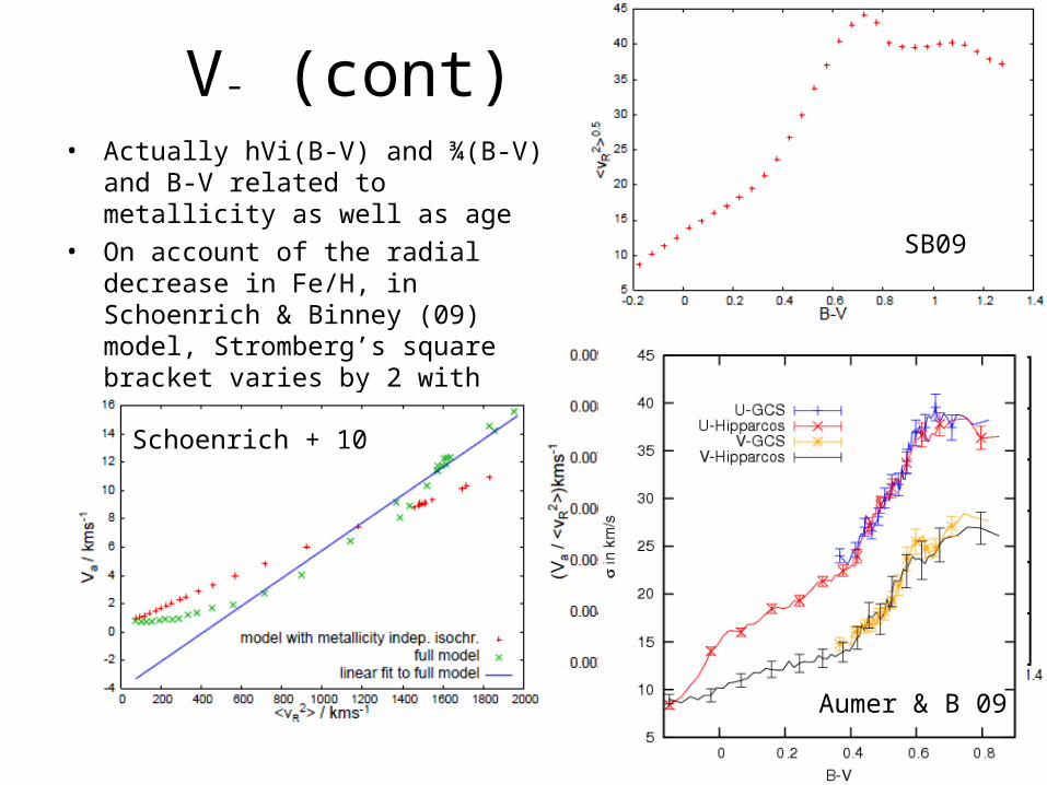
V¯ (cont)• Actually hVi(B-V) and ¾(B-V) and B-V
related to metallicity as well as age
• On account of the radial decrease in Fe/H, in Schoenrich & Binney (09) model, Stromberg’s square bracket varies by 2 with colour
SB09
Aumer & B 09
Schoenrich + 10

V¯ (cont)
• Safer to fit theoretical U, V, W distribs to data
• Conclude V¯=12§2 km/s
Conclusions
• Urgent requirement for hierarchy of models that incorporate dynamics & chemistry
• Important to know DF• Torus dynamics seems to fit the bill• Basic reference models have analytic DFs• Fit to current data imperfect but data rather than models
may be at fault• Next steps
– fit in space of observables (MV, , ¹, l, b) taking proper account of inhomogeneous errors
– Upgrade SB09 dynamics• Use tori• Securer basis for scattering probabilities


