Download - The Collateral Channel - TSE
The Collateral Channel:How Real Estate Shocks affect Corporate Investment∗
Thomas Chaney† David Sraer‡ David Thesmar§
August 15, 2011
Abstract
What is the impact of real estate prices on corporate investment? In the presenceof financing frictions, firms use pledgeable assets as collateral to finance new projects.Through this collateral channel, shocks to the value of real estate can have a large impacton aggregate investment. Over the 1993-2007 period, the representative U.S. corporationinvests $.06 out of each $1 of collateral. To compute this sensitivity, we use local variationsin real estate prices as shocks to the collateral value of firms that own real estate. Weaddress the endogeneity of local real estate prices using the interaction of interest ratesand local constraints on land supply as an instrument. We address the endogeneity of thedecision to own land (1) by controlling for observable determinants of ownership and (2)by looking at the investment behavior of firms before and after they acquire land. Thesensitivity of investment to collateral value is stronger the more likely a firm is to be creditconstrained.
∗We are grateful to Institut Europlace de Finance for financial support. For their helpful comments, wewould like to thank Nicolas Coeurdacier, Stefano DellaVigna, Denis Gromb, Luigi Guiso, Thierry Magnac,Ulrike Malmendier, Atif Mian, Adam Szeidl and Jean Tirole, as well as two anonymous referees and the Editor.We are especially indebted to Chris Mayer, for providing us with the Global Real Analytics data. We are alsograteful to seminar participants at INSEE in Paris, USC, UC San Diego Rady School of Management, NYUStern, MIT Sloan, the University of Amsterdam, London Business School, Oxford’s Saïd School of Business, theUniversity of Chicago, the European University Institute in Florence, Bocconi University, Toulouse School ofEconomics, the Kellogg School of Management, Princeton University, the Haas School of Business at Berkeley,and the University of Naples. We are solely responsible for all remaining errors.†University of Chicago, NBER and CEPR,[email protected]‡Princeton University, [email protected]. Corresponding Author: 26 Prospect Avenue, Princeton, NJ
08540.§HEC Paris and CEPR,[email protected]
1

1 IntroductionIn the presence of contract incompleteness, Barro (1976), Stiglitz and Weiss (1981) and Hartand Moore (1994) point out that collateral pledging enhances a firm’s debt capacity. Providingoutside investors with the option to liquidate pledged assets ex post acts as a strong discipliningdevice on borrowers. This, in turn, eases financing ex ante. Asset liquidation values thusplay a key role in the determination of a firm’s financing capacity. This simple observationhas important macroeconomic consequences: as noted by Bernanke and Gertler (1989) andKiyotaki and Moore (1997), business downturns will deteriorate assets values, thus reducingdebt capacity and depressing investment, which will amplify the downturn. This “collateralchannel” is often the main suspect for the severity of the Great Depression (Bernanke (1983)) orfor the extraordinary expansion of the Japanese economy at the end of the 80’s (Cutts (1990)).In the current context of abruptly declining real estate prices in the U.S., an assessment of therelevance of this “collateral channel” is called for. This paper attempts to empirically uncoverthe microeconomic foundation for this mechanism.
We show that over the 1993-2007 period, a $1 increase in collateral value leads the rep-resentative U.S. public corporation to raise its investment by $.06. This sensitivity can bequantitatively important in the aggregate. This is because real estate represents a sizable frac-tion of the tangible assets that firms hold on their balance sheet. As we show in this paper, in1993, among public firms in the US, 58% reported at least some real estate ownership. Amongthese land-owning firms, our estimation of the value of real estate holdings represented some20% of shareholder value.
To get at this $.06 sensitivity, we use variations in local real estate prices, either at the stateor the city level, as shocks to the collateral value of land holding firms. We measure how a firm’sinvestment responds to each additional dollar of real estate that the firm actually owns, and nothow investment responds to real estate shocks overall. This empirical strategy uses two sourcesof identification. The first comes from the comparison, within a local area, of the sensitivity ofinvestment to real estate prices across firms with and without real estate. The second comesfrom the comparison of investment by land holding firms across areas with different variationsin real estate prices. The methodology is similar to Case et al. (2001) in their study of homewealth effects on household consumption.
Two sources of endogeneity might affect our estimation. First, real estate prices may becorrelated with the investment opportunities of land holding firms. We instrument local realestate prices using the interaction of long-term interest rates (to capture time variations inhousing demand) with local housing supply elasticity (see Himmelberg et al., 2005, and Mianand Sufi, 2009, for a use of these elasticities). The second endogeneity issue is that the decisionto own or lease real estate may be correlated with the firm’s investment opportunities or theextent of its credit constraints (Eisfeldt and Rampini, 2009, and Rampini and Vishwanathan,2010). We do not have a proper set of instruments to deal with this problem, but we make twoattempts at gauging the severity of the bias it may cause. We first control for the observabledeterminants in the ownership decision, which leaves the estimation unchanged. Second, weestimate the sensitivity of investment to real estate prices for firms that acquire real estatebefore and after they do so. Before acquiring real estate, future purchasers are statisticallyindistinguishable from firms that never own real estate. The sensitivity of their investment to
2

real estate prices becomes large, positive and significant only after they acquire real estate.This paper is a contribution to the emerging empirical literature on collateral and investment.
The seminal paper in this literature is Peek and Rosengreen (1997), who look at the supply sideof credit. During the collapse of the Japanese real estate bubble in the early 1990s, they showthat banks owning depreciated real estate assets cut their credit supply in the US, leading toa decrease in their clients’ investment.1 Closest to our paper is Jie Gan (2007a) who showsthat land holding Japanese firms were more affected by the burst of the real estate bubble inthe beginning of the 90s than firms with no real estate. By contrast, our identification rests on“normal” real estate market conditions over nearly 20 years of data. Our estimates thus reflect“normal” firm behavior and not the response to the collapse of one of the largest property bubblesin History. Besides, we address some of the shortcomings of her important study. First, sinceshe focuses on a single macro event, her estimates are vulnerable to confounding macro-effects(exchange rate variations, stock market collapse, etc.).2 Second, we study the US, an economywhere banks, and hence collateral, may play a smaller role. Another advantage of looking atthe US is that our paper uses widely available data and our methodology is easy to implementin future research.3
Finally, our paper is also closely related to recent work that try to highlight the role ofcollateral in financial contracts. Benmelech, et al. (2005) document that more liquid (or more“redeployable”) pledgeable assets are financed with loans of longer maturities and durations.Benmelech and Bergman (2008) documents how U.S. airline companies are able to take advan-tage of lower collateral value to renegotiate ex post their lease obligation downward. Finally,Benmelech and Bergman (2009) construct industry-specific measures of redeployability and showthat more redeployable collateral leads to lower credit spreads, higher credit ratings, and higherloan-to-value ratios. While we do not go into such details in the examination of financial con-tracts, our paper contributes to this literature by empirically emphasizing the importance ofcollateral for financing and investment decisions.4
The remainder of the paper is organized as follows. Section 2 presents the construction ofthe data and summary statistics. Section 3 describes our main empirical results on investmentand capital structure decisions. Section 4 concludes.
2 DataWe use accounting data on US listed firms, merged with real estate prices at the state andMetropolitan Statistical Area (MSA) level.
1Gan (2007b) also uses the Japanese crisis as a shock to banks health and identifies the importance of bankhealth on their clients’ investment.
2One of her robustness checks looks at cross-sectional variations in land prices, but, as pointed out in thepaper, the dispersion of price changes in the cross section is too small to provide meaningful identification.
3Another contribution looking at collateral shocks triggered by the Japanese crisis can be found in Goyal andYamada (2001).
4For other contributions emphasizing the role of collateral in boosting pledgeable income, see, among others,Eisfeldt and Rampini (2009) and Rampini and Viswanathan (2010)
3

2.1 Accounting Data
We start from the sample of active COMPUSTAT firms in 1993 with non-missing total assets(COMPUSTAT item #6). This provides us with a sample of 9,211 firms and a total of 83,719firm-year observations over the period 1993 - 2007. We keep firms whose headquarters are locatedin the United States and exclude from the sample firms operating in the finance, insurance,real estate, construction and mining industries, as well as firms involved in a major takeoveroperation. We keep firms that appear at least three consecutive years in the sample. This leavesus with a sample of 5,121 firms and 51,467 firm year observations.
2.1.1 Real Estate Assets
We collect data on the value of real estate assets of each firm. After measuring the initial marketvalue of real estate assets of each firm, we will identify variations in their value coming fromvariations in real estate prices across space and over time.
First, we measure the market value of real estate assets. Following Nelson et al. (1999),three major categories of property, plant and equipments are included in the definition of realestate assets: Buildings, Land and Improvement and Construction in Progress. Unfortunately,these assets are not marked-to-market, but valued at historical cost. To recover their marketvalue, we calculate the average age of those assets, and use historical prices to compute theircurrent market value. The procedure is as follows. The ratio of the accumulated depreciationof buildings (COMPUSTAT item #253) to the historic cost of buildings (COMPUSTAT item#263)5 measures the proportion of the original value of a building claimed as depreciation.Based on a depreciable life of 40 years,6 we compute the average age of buildings for each firm.Using state-level residential real estate inflation after 1975, and CPI inflation before 1975, wecompute the market value of real estate assets for each year in the sample period (1993-2007).
The accumulated depreciation on buildings is no longer available in COMPUSTAT after1993.7 This is why, when measuring the value of real estate, we restrict our sample to firmsactive in 1993. There are 2,750 firms in 1993 in our sample for which we are able to construct ameasure of the market value of real estate assets and 28,014 corresponding firm-year observations.Table 1 reveals two striking facts. In 1993, 58% of all US public firms reported some real estateownership. Moreover, for the median firm in the entire sample, the market value of real estaterepresents 30% of the book value of Property, Plants and Equipment (and 5% of the firm’s totalmarket value). For the median land holding firm in COMPUSTAT, the market value of realestate represents 98% of the book value of Property, Plant and Equipment and 19% of the firm’stotal market value. Real estate is thus a sizable fraction of the tangible assets that corporationshold on their balance sheet.
5Unlike buildings, land and improvements are not depreciated.6As in Nelson et al. (1999), this assumption can be tested by estimating annual depreciation amounts (as
the change in total depreciation). Building cost, when divided by annual depreciation, provides an estimate ofdepreciable life. Although inconsistent, the average life estimated by this approach ranges from 38 to 45 years.This confirms our assumption of a 40-year-life.
7In 1994, ten of the fifteen schedules required for Electronic Data Gathering, Analysis and Retrieval system(EDGAR) filings were eliminated. In particular, the accumulated depreciation on Buildings is no longer reported.
4

Second, to measure accurately how the value of real estate assets evolves, we need to knowthe location of these assets. COMPUSTAT does not provide us with the geographic locationof each specific piece of real estate owned by a firm. However, the data reports headquarterlocation (variables STATE and COUNTY). We use the headquarter location as a proxy for thelocation of real estate. There are two assumptions underlying this choice. First, headquartersand production facilities tend to be clustered in the same state and MSA. Second, headquartersrepresent an important fraction of corporation real estate assets. To support these assumptions,we manually collected information on the location of a firm’s real estate using their 10K files.We discuss these data in detail in section 2.3.
2.1.2 Other Accounting Data
Aside from data on real estate, we use other accounting variables, and construct ratios as istypically done in the corporate finance literature. We compute the investment rate as the ratioof capital expenditures (COMPUSTAT item #128) to past year’s Property Plant & Equipment(item #8).8 We compute the Market-to-Book ratio as follows: we take the total market valueof equity as the number of common stocks (item #25) times end-of-year close price of commonshares (item #24). To this, we add the book value of debt and quasi equity, computed as bookvalue of assets (item #6) minus common equity (item #60) minus deferred taxes (item #74).We then normalize the resulting firm’s “market” value using book value of assets (item #6). Wealso use the ratio of cash flows (item #18 plus item #14) to past year’s PPE (item #8).
We use COMPUSTAT to measure debt issuance. We measure long term debt issues aslong term debt issuance (item #111) normalized by lagged PPE (item #8). We also computelong term debt repayment (item #114) divided by lagged PPE. Finally, only the net changein current debt (item #301) is available in COMPUSTAT, and we also normalize it by laggedPPE. Net change in long term debt is defined as long term issuance minus long term repaymentsnormalized by PPE. Because data on issuances and repayments are sometimes missing, we alsocompute net change in long term debt as the yearly difference in long term debt normalized bylagged PPE.
In most of the regression analysis, we use initial characteristics of firms to control for thepotential heterogeneity among our 2,750 firms. These controls, measured in 1993, are based onReturn on Assets (operating income before depreciation (item #13) minus depreciation (item#14) divided by total assets (item #6)), Assets (item #6), Age measured as number of yearssince IPO, 2-digit SIC codes and state of location.
Finally, to ensure that our results are statistically robust, all variables defined as ratiosare windsorized at the 5th percentile.9 Table 1 provides summary statistics on most accountingvariables used in the paper. We simply remark that the debt-related variables (Debt Repayment,Debt Issues, Net Debt Issues and Changes in Current Debt) have high means (.75 for debt issues,for instance) but fairly low medians (e.g., .01 for debt issues). This is because (1) these variables
8This normalization by PPE is standard in the investment literature (see, e.g., Kaplan and Zingales (1997)or Almeida et al. (2007)). It provides typically a median investment ratio of .21. An alternative specification isto normalize all variables by lagged asset value (item #6), as in Rauh (2006) for instance, which deliver notablylower ratios. Our results are robust to this alternative normalization choice.
9Windsorizing at the first percentile or trimming the variables at the 5th/1st percentile does not qualitativelychange our results.
5

are normalized by lagged PPE, which is notably smaller than total asset and (2) these variablesare left censored so that they are naturally right-skewed and as a consequence, our windsorizingmethodology still leaves an important mass on the right tail of these distributions.
2.1.3 Ex-Ante Measure of Credit Constraint
The standard empirical approach in the investment literature uses ex ante measures of financialconstraint to sort between “Constrained” and “Unconstrained” firms. Estimations are performedseparately for each set of firms. We follow Almeida et al. (2004) in this approach and definethree measures of credit constraint using the following schemes:
• Payout ratio: In every year over the 1993 - 2007 period, we rank firms based on their payoutratio and assign to the financially constrained (unconstrained) group those firms in thebottom (top) three deciles of the annual payout distribution. We compute the payout ratioas the ratio of total distributions (dividends plus stock repurchases) to operating income.
• Firm Size: In every year over the 1993 - 2007 period, we rank firms based on their totalassets and assign to the financially constrained (unconstrained) group those firms in thebottom (top) three deciles of the annual asset size distribution.
• Bond Rating: In every year over the 1993 - 2007 period, we retrieve data on bond ratingsassigned by Standard & Poor’s and categorize those firms with debt outstanding butwithout a bond rating as financially constrained. Financially unconstrained firms arethose whose bonds are rated.
2.2 Real Estate Data
2.2.1 Real Estate Prices
We use data on residential and commercial real estate prices, both at the state and at the MSAlevel.
Residential real estate prices come from the Office of Federal Housing Enterprise Over-sight.1011 The O.F.H.E.O. provides a Home Price Index (HPI), which is a broad measure of themovement of single-family home prices in the US.12 Because of the breadth of the sample, itprovides more information than is available in other house price indices. In particular, the HPIis available at the state level since 1975. It is also available for most Metropolitan Statistical Ar-eas, with a starting date between 1977 and 1987 depending on the MSA considered. We matchthe state level HPI with our accounting data using the state identifier from COMPUSTAT. To
10http://www.ofheo.gov/index.asp11The O.F.H.E.O. is an independent entity within the Department of Housing and Urban Development, whose
primary mission is “ensuring the capital adequacy and financial safety and soundness of two government-sponsoredenterprises (GSEs) - the Federal National Mortgage Association (Fannie Mae) and the Federal Home LoanMortgage Corporation (Freddie Mac)”.
12The HPI is computed using a hedonic regression and each release of the HPI offers a different value of theindex for a given state year. The results presented in the paper are not, however, significantly different if, forinstance, we use the 2006 release instead of the 2007 release.
6
match the MSA level HPI, we aggregate FIPS codes from COMPUSTAT into MSA identifiersusing a correspondence table available from the OFHEO website.
Commercial real estate prices come from Global Real Analytics. This dataset provides aprice index for Offices and Industrial Commercial Real Estate.13 This index is only available fora subset of 64 MSAs in the U.S. with a starting date between 1985 and 2003.
Table 1 provides details on these indices (that have been normalized to 1 in 2006). Thecorrelation between the residential and commercial indices at the state level is .57, and .42 atthe MSA level. The correlation between the two residential indices is .86.
2.2.2 Measuring Land Supply
Controlling for the potential endogeneity of local real estate prices in an investment regression isan important step in our analysis. Following Himmelberg et al. (2005), we instrument local realestate prices using the interaction of long-term interest rates and local housing supply elasticity.Local housing supply elasticities are provided by Saiz (2009) and are available for 95 MSAs.These elasticities capture the amount of developable land in each metro area and are estimatedby processing satellite-generated data on elevation and presence of water bodies. As a measureof long-term interest rates, we use the “contract rate on 30 year, fixed rate conventional homemortgage commitments” from the Federal Reserve website, between 1993 and 2007.
2.3 Measurement Issues
The empirical methodology we use in this paper relies on several approximations that introducemeasurement errors in the regression analysis. In this Section, we present evidence in supportof these approximations.
The first approximation we make relates to the location of firms’ real estate assets. We as-sume that firms own most of their real estate assets in the state (or MSA) where their headquar-ters are located. We do so because there is no systematic source of information on corporations“true” location(s). To check the validity of this approximation, we manually collected informa-tion on the ownership status of a firm’s headquarter from the 10K forms filed with the Securityand Exchange Commission for the year 1997.14 These documents were retrieved from the SEC’sEDGAR website (http://www.sec.gov/edgar.shtml). Information on a firm’s headquartersownership was available for 4,065 firms in 1997.15 Of those firms, 3,436 firms also have nonmissing information on the value of their real estate assets in COMPUSTAT.16
13We use the Offices index in our analysis but the main results are left unchanged if we use the Industrialindex instead.
141997 is the earliest date for which 10K forms are available on the web. We also collected the same informationfor the year 2000, which we used in our study of the real estate bubble of the early 2000’s in Section 3.7.
154,065 firms reported in their 10K files a single headquarter. In addition, 164 firms reported 2 distinctheadquarters, and 19 reported 3 or more headquarters. These cases of multiple headquarters seem to typicallycorrespond to small firms that have both their headquarters in either a small city, or in the suburb of a largecity, and in addition, have an address in a large city that they use primarily as a mailing address (in some ofthose 183 cases, we could explicitly identify the address for the second headquarter as a PO box). We droppedthose few observations with multiple headquarters.
16The corresponding numbers for 2000 are: 2,902 firms with non missing real estate information in COMPU-STAT out of 3,666 firms with available 10K files.
7

For those 3,436 firms, it is possible to check how the 10K information on HQ ownership andthe COMPUSTAT information on land ownership match. Table 2 provides the evidence. Ofthe 1,606 firms that report owning no real estate assets in COMPUSTAT, only 34 firms (2%)report owning their headquarters in their 10K forms. Hence, the probability of missing a realestate owner using COMPUSTAT information is small.
On the other hand, of the 1,830 firms that report owning some real estate assets in COM-PUSTAT, only 806 (44%) actually report owning their headquarters in their 10K forms.17 Theassumption that all of the real estate assets of a firm are located in its headquarters’ State orMSA is not validated in the data. However, we remark that this will mechanically lead us tounderestimate the magnitude of our effect. If a firm owns real estate assets outside its head-quarters’ MSA, we overestimate the fraction of the value of its real estate assets that co-moveswith real estate prices in this MSA. This leads to underestimate the effect of a dollar increase incollateral value on investment. We point out in Section 3 that using an ownership dummy usingCOMPUSTAT information or an ownership dummy using 10K information yields very similarresults. Thus, this particular measurement error does not seem to bias our results significantly.
Second, using the OFHEO residential real estate prices as a proxy for commercial real estateprices could be a source of noise in our regression. As noted earlier, the correlation betweenthe two indices ranges from .42 (at the MSA level) to .57 (at the State Level). Moreover, thecommercial index is available only at the MSA level, and for a subset of cities. Therefore, thereis a trade-off: this index corresponds more accurately to the true nature of firms real estateassets but it relies on the stronger assumption that these assets are mostly located in the citywhere headquarters are located. We present evidence using both series of prices (residential andcommercial) and show that our results do not depend on the price index used.
3 Real Estate Prices and Firm BehaviorIn this Section we analyze the impact of real estate shocks on corporate investment. Our goal isto provide an estimate of the financial multiplier (i.e. by how much an increase in assets’ valueincreases investment) at the firm-level.
3.1 Empirical Strategy
We run different specifications of a standard investment equation. Specifically, for firm i, atdate t, with headquarters in location l (State or MSA), investment is given by:
INV lit = αi + δt + β.RE V alueit + γP l
t + controlsit + εit (1)
where INV is the ratio of investment to lagged PPE, RE V alueit is the ratio of the marketvalue of real estate assets in year t to lagged PPE and P l
t controls for the level of prices inlocation l (State or MSA) in year t.
The interpretation of this reduced form equation is based on a simple model of investment17Note that a firm may not own its headquarters, but may still own other real estate assets in its headquarters
State or MSA.
8

under collateral constraint.18 In the presence of financing constraints, at least a fraction of firmswill use their pledgeable assets as collateral to finance their investment. A constrained firm willborrow a fraction the collateral value of all its pledgeable assets. Conditional on not defaultingon its debt at the end of a period, a firm will repay its debt, and then use its collateral again tofinance investment in the subsequent period. This model justifies our choice of regressing theannual investment of a firm on the current market value of its entire stock of real estate assets.The estimated coefficient β̂ is a composite measure of the fraction of firms in the sample thatface financing constraints, the severity of these financing constraints, and the fraction of thevalue of real estate assets that can be used as collateral. If the coefficient β̂ is positive, then atleast some firms face financing constraints. In a reduced form, this coefficient β̂ measures, forthe average firm in the sample, the fraction of its collateral that is used to finance investment.
As is typically done in the reduced-form investment literature, we control for the ratio of cashflows to PPE and the one year lagged market to book value of assets. We also include a firmfixed effect αi, as well as year fixed effects δt, designed to capture aggregate specific investmentshocks, i.e. fluctuations in the global economy. Finally, the variable P l
t controls for the overallimpact of the real estate cycle on investment, irrespective of whether a firm owns real estateor not. Shocks εit are clustered at the State/MSA × year level. This correlation structure isconservative given that the explanatory variable of interest RE V alueit is defined at the firmlevel (see Bertrand, Duflo and Mullainathan [2004]).
As noted in Section 2.1.1, the market value of the entire real estate portfolio of a firm canonly be estimated before 1993, which is the last year for which accumulated depreciations onbuildings are available. RE V aluei1993 is thus defined as the initial market value of a firm’sreal estate assets, and subsequent variations in RE V alueit capture fluctuations in the marketvalues of these specific assets.19
Let us also highlight that the coefficient β measures how a firm’s investment responds toeach additional $1 of real estate the firm actually owns, and not how investment responds toreal estate shocks overall. This specification allows us to abstract from state-specific shocks thatwould affect both firms with and without real estate assets.
Endogeneity Issues
There are two potential sources of endogeneity in the estimation of equation (1): (1) real estateprices could be correlated with investment opportunities and (2) the ownership decision couldbe related with investment opportunities.
There are two immediate reasons why real estate prices could be correlated with investmentopportunities. The first one is a simple reverse causality argument: large firms might have a
18In our online Appendix, we develop a simple model of investment under collateral constraint to justify thisspecification. This version is available at www.princeton.edu/ dsraer/theoryRE.pdf.
19Using only the initial value of real estate in 1993 offers an additional advantage: if a firm discovers a profitableinvestment opportunity, and if it leases some of its real estate, we may expect that its landlord will try to extractas much rent as possible from this future investment; to escape from this hold-up problem, we may expect thisfirm to become owner of its real estate exactly when it is about to invest; in such a scenario, we would then see aspurious correlation between the current value of the real estate a firm owns and its investment. We circumventthis problem by using variations in the value of real estate that come only from market prices, and not from thecontemporaneous strategy of the firm.
9

non negligible impact through the demand for local labor and locally produced intermediateson the local activity, so that an increase in investment for such large, land holding firms, couldtrigger a real estate price appreciation. This would lead us to over-estimate β. Second, it couldbe that our measure of real estate prices proxies for local demand shocks, and that, for somereason, land holding firms are more sensitive to local demand.
To address this source of endogeneity, we instrument MSA level real estate prices. As alreadymentioned in Section 2.2.2, we do so by interacting local housing elasticities with aggregateshifts in the interest rate. When interest rates decrease, the demand for real estate increases.If the local supply of land is very elastic, the increased demand will translate mostly into moreconstruction (more quantity) rather than higher land prices. If the supply of land is very inelasticon the other hand, the increased demand will translate mostly into higher prices rather thanmore construction. We expect that in MSAs where land supply is more constrained, a drop ininterest rate should have a larger impact on real estate prices (our first-stage regression). Wethus estimate, for MSA l, at date t, the following equation predicting real estate prices P l
t :
P lt = αl + δt + γ.Elasticityl × IRt + ul
t (2)
where Elasticity measures constraints on land supply at the MSA level, IR is the nationwidereal interest rate at which banks refinance their home loans. αl is an MSA fixed effect, and δtcaptures macroeconomic fluctuations in real estate prices, from which we want to abstract.
To further address this concern, we verify in Section 3.3 that our results are robust torestricting our sample to small firms (bottom 3 quartiles of book value of assets) in large cities(top 20 MSAs in terms of population). In those cases, we do not expect any individual firm tohave a sizable impact on local real estate prices through a general equilibrium feedback.
The second source of endogeneity in the estimation of equation (1) comes from the ownershipdecision: if firms that are more likely to own real estate are also more sensitive to local demandshocks, we would over-estimate β. As a first step in addressing this issue, we control for initialcharacteristics of firm i, Xi, interacted with real estate prices Pm
t . If those controls identifycharacteristics that make firm i more likely to own real estate, and if those characteristics alsomake firm i more sensitive to fluctuations in real estate prices, controlling for the interactionbetween those controls and the contemporaneous real estate prices allows to separately identifythe collateral channel we are interested in.
The Xi are controls that we believe should play an important role in the ownership decisionand include 5 quintiles of Age, Assets and Return on Assets as well as 2-digit industry dummiesand State dummies. We show in Table 3 that these characteristics are good predictors of thedecision to buy real estate assets and, to a lesser extent, on the amount of real estate purchased.Table 3 is a simple cross-sectional OLS regression of RE OWNER, a dummy equal to 1 whenthe firm owns real estate, and RE V alue, the market value of the firm’s real estate assets, onthe initial characteristics mentioned above. Older, larger and more profitable firms, i.e. maturefirms, are more likely to be owners in our dataset.20
20Note that, from an intuitive perspective, these firms seem to be more likely to be insulated from local demandshocks. This suggests that the hypothesis according to which land holding firms are inherently more likely to beaffected by local demand shocks is far from evident in the data.
10

Controlling for the observed determinants of real estate ownership, we estimate the followingreduced form investment equation:
INV lit = αi + δt + β.RE V alueit + γP l
t +∑
k
κk.Xik × P l
t + controlsit + εit (3)
However, some determinants of the land holding decisions might not be observable, whichmakes our approach in equation (3) insufficient. Unfortunately, it is difficult to find firm-levelinstruments that predict real estate ownership. Yet, it is possible to control for firm-levelcorrelation between investment and real estate prices, as long as it is fixed over time. To doso, we look in Section 3.6 at the sensitivity of investment to real estate prices for firms thatare about to purchase a property, but before the purchase. If the unobserved characteristicsthat co-determine investment and ownership is time invariant, then it should be the case thatfirms that are about to purchase real estate assets are already more sensitive to the real estatecycle. Section 3.6 shows that this is not the case, and describes the implementation of thistest in greater details. We insist however that while suggestive, this approach is by no meansdefinitive, as the unobserved heterogeneity could well vary over time, making the approach inSection 3.6 irrelevant.
3.2 Main Results
Table 4 reports estimates of various specifications of equation (1) and (3). Column (1) startswith the simplest estimation of equation (1) without any additional controls. Land holding firmsincrease their investment more than non land holding firms when real estate prices increase. Thebaseline coefficient is .077, so that each additional $1 of real estate collateral increases investmentby $.077. The coefficient is significant at the 1% confidence level. The effect is economicallylarge: a one s.d. increase in RE V alue increases investment by 28% of investment’s s.d.21
In Column (2), we add the initial controls interacted with real estate prices that account forthe observed heterogeneity in ownership decisions and its potential impact on the sensitivity ofinvestment to real estate prices. The coefficient is now .067, still significant at the 1% confidencelevel, somewhat smaller but not statistically different from .077 found in column (1).
Column (3) adds state variables traditionally used in estimating investment equations, i.e.Cash and Market to Book. Simple theory suggests that, if collateral constraints matter, theestimated coefficient on RE V alue should decrease but remain positive. Intuitively, to leavethe Market-to-Book ratio unchanged after a positive shock to the value of the firm’s real estateassets, there need to be a negative shock to unobserved productivity. This negative shockto productivity generates a negative shock to investment. As a consequence, the response ofinvestment to the initial shock in real estate prices will be smaller than it would have beenhad the Market-to-Book ratio not been controlled for.22 The reduced form sensitivity remainspositive but is now smaller, equal to .055.23 A one s.d. increase in collateral value explains a
21Increasing RE V alue by one s.d. (1.36) increases INV by .077 × 1.36 = .10, which represents 28% ofinvestment’s s.d. (.37).
22We derive this intuition formally in our simple model presented in the online appendix.23In particular, in unreported regressions, we see that most of the drop in the sensitivity comes from adding
the control for the Market-to-Book ratio and not from adding Cash.
11

20% s.d. increase in investment once the effect of the Market to Book and the other controls areaccounted for. Note that, as is traditional in the investment literature, both Cash and Marketto Book have a significant, positive impact on investment.
Column (4) replicates the estimation performed in Column (3) using the MSA-level residen-tial price index instead of the State-level index. Using MSA level prices has both advantagesand drawbacks. It offers a more precise source of variation in real estate prices. It also makesour identifying assumption that investment opportunities are uncorrelated with variations inlocal prices milder. However, there are potentially larger measurement errors, as we now rely onthe assumption that all the real estate assets that a firm owns are located in the headquarters’city. The results in Column (4) show that the coefficient remains stable, at .055.
Column (5) uses commercial real estate prices instead of residential prices. The lower numberof MSA’s with available commercial real estate prices reduces slightly the number of observations(18,080 observations compared to 23,222 in the specification using MSA residential prices).However, the sensitivity remains strongly positive and significant at the 1% level, and is slightlyhigher than that computed using residential prices: a $1 increase in the value of commercial realestate assets leads to an average increase of $.064 in investment.
Column (6) implements the I.V. strategy where real estate prices are instrumented using theinteraction of interest rates and local constraints on land supply (see Section 3.1). Let us firstbriefly comment the first stage regressions, which are direct estimations of equation (2). Theseestimations are presented in Table 5. The first two columns predict MSA residential prices,while the two last columns predict MSA office prices. In column (1) and (3), we directly use themeasure of local housing supply elasticity provided in Saiz (2009). In column (2) and (4), wegroup MSAs by quartile of local housing supply elasticity.
Low values of local housing supply elasticity correspond to MSAs with very constrained landsupply. We expect the positive effect of declining interest rates on prices to be stronger in MSAswith less elastic supply. As expected, the γ coefficient in equation (2) is positive and significantat the 1% confidence level. For instance, using the results in Column (4), a 100 basis pointsinterest rate decline increases the office price index by 6 percentage points more in “constrained”cities (top quartile of the elasticity distribution) than in “unconstrained” cities (bottom quartile).These effects are economically large, and significant. All F-tests for nullity of the instrumentare above 10 which leads us to conclude that these instruments are not weak.
Moving to the second stage equation, we simply use predicted prices P̂ lt from the estimation
of equation (2) and use them as an explanatory variable in equation 3.24 Column (6) in Table4 reports the result of the estimation when the instrument used in the first stage is the local
24Because we construct our set of predicted prices on a different sample than the sample over which we runour investment regression, we need to adjust our standard errors to account for this predicted regressor. In allour IV specification, we thus report bootstrapped t-stats. The bootstrap has been done as follows: we first drawa random sample with replacement within the sample of MSA-years; we run the first-stage regression on thissample; we then draw another random sample with replacement within the sample of firm-years; to correct forthe correlation structure of this sample (MSA-year), this random draw is made at the MSA-year level, and notat the firm-year level (i.e. we randomly draw with replacement a MSA-year and then select all the firms withinthis MSA-year); we finally run our second-stage regression on this sample. We repeat this procedure 1000 timesand the standard-error we report is calculated from the empirical distribution of the coefficients estimated.
12

housing supply elasticity (i.e. Column (3) of Table 5). The coefficient estimated from this IVregression is very close to the one obtained from the OLS regression, equal to .065 and remainssignificant at the 1% level.
Column (7) tests whether the relation between collateral value and investment found incolumns (1)-(5) depends on the shape of the empirical distribution of collateral values. To doso, we interact the RE OWNER dummy (equal to 1 when a firm owns some real estate assetsin 1993) with the real estate price index. The estimated coefficient is positive and stronglysignificant, indicating that our results are not driven by firms with large real estate holdings.Of course, the interpretation of the coefficient on this dummy specification (RE OWNER)is not directly comparable to the one with the continuous variable (RE V alue). While the.064 coefficient in Column (5) means that a $1 increase in the value of a firm’s real estateassets translates into a $.064 increase in investment, the .21 coefficient in Column (7) meansthat, on average, a firm that owns at least some real estate increases its investment rate by 21percentage points more than a firm that does not own real estate when the local price indexdoubles (increases from 1 to 2). However, the economic magnitude implied by this dummyspecification is very similar to the specification that uses the value of real estate, as in column(5). A one s.d. increase in the interaction between the dummy RE OWNER and land prices(resp. RE V alue) increases investment by 22% (resp. 22%) of investments s.d.25
Column (8) implements the I.V. strategy on the dummy specification of column (7). In thatspecification, the sensitivity of investment to real estate prices for owners versus non ownersincreases almost two-fold, from .21 to .46. The estimated coefficient remains significant at the1% confidence level.
3.3 Robustness checks
Table 6 provides various robustness checks of the baseline estimation of equation (3) in column(5) of Table 4.
Column (1) and (2) reproduce the estimation on two different subsample periods: before1999 in column (1), and after 2000 in column (2). A potential issue with pooled regressions asthe ones presented in Table 4 is that they might conceal a fair amount of heterogeneity in theelasticity over time. We find that the estimated coefficients are significant in both sub-periods.The estimated coefficient β̂ is only marginally higher before 1999 than after 2000 (.085 versus.084), and not statistically different. Neither the significance nor the magnitude of the coefficientof interest does seem to come from some particular years in our sample.
Column (3) estimates equation (3) on a sub-sample of small firms in large MSA’s. Thisspecification addresses the concern of reverse causality, whereby a large firm’s investment mayincrease local real estate prices. We consider only firms in the lower three quartiles of size (bookvalue of assets), and in the top 20 MSAs in terms of population. The estimated coefficient
25The coefficient β for the dummy specification in Column (7) is .21, and one standard deviation of the RHSvariable RE Owner×MSA office prices is .39, so that .21×.39 ≈ .082 represents 22.1% of investment’s s.d. (equalto .37). The coefficient β for the comparable continuous specification in Column (5) is .064, and one standarddeviation of the RHS variable RE V alue is 1.26, so that .064× 1.26 ≈ .081 represents 21.8% of investment’s s.d(.37).
13

remains significant at the 1% confidence level, and is only marginally smaller than, but notstatistically different from, the coefficient estimated on the entire sample (.061 compared to.064).
Column (4) uses as a dependent variable variations in PPE net of variations in real estate.One possible concern may be that investment includes investment in real estate assets. If a firmwere to systematically acquire real estate assets when real estate prices increase, and all themore so if that firm already owns more real estate, one would mechanically find a coefficientβ.26 Removing any acquisition or sales of real estate from investment addresses this concern.The estimated coefficient remains large and significant at the 1% level.27
Column (5) uses as a dependent variable the average investment over the subsequent threeyears, as opposed to the current investment over a single year. One may expect that in thepresence of collateral constraints, the renegotiation of debt contract with lenders following anappreciation of a firm’s real estate may be gradual. As expected, the coefficient increases from$.064 to $.09 of investment for each additional $1 of collateral. In her study of 1990s Japan, JieGan (2007a) finds a .8 percentage points decrease in investment for a 10% drop in real estatevalue. In our context, we obtain that a 10% decrease in REV alue around its sample mean(0.083 ppoints) leads to an investment reduction by .09× 8.3 = .7 percentage points. The twoestimates are remarkably close.
Column (6) uses as dependent variable the investment of firm i adjusted for the overallinvestment of firms in i’s 2-digit SIC code. Such a specification addresses the concern thatinvestment may be concentrated in specific sectors where firms tend to own their real estate,and that those sectors may have been concentrated in areas that experienced large real estateprice inflation. The coefficient of interest remains unchanged at $.064 of investment per $1 ofcollateral, and remains significant at the 1% level.
Column (7) uses the entire sample of firms, without restricting our attention to firms thatwere present in our sample in 1993. This specification addresses the possible concern thatselection and survivorship bias may lead to biased estimates. Of course, as explained in Section2.1.1, the information on the accumulated depreciation on buildings that we use to constructthe market value of real estate assets is not available after 1993. For firms that enter our datasetafter 1993, we only know whether they own real estate or not, but not the market value of theirreal estate assets. We therefore re-estimate the dummy specification of equation (3), but usingthe extended sample. The results of this regression in column (7) of Table 6 are to be comparedto the similar regression in column (7) of Table 4. The coefficient of interest is unchanged (.21),and remains statistically significant at the 1% level in this unrestricted sample.
Column (8) uses the information on whether a firm actually owns its headquarters directlyfrom the 10K files for the year 1997.28 The collection of this data is described in Section 2.3.
26In unreported regressions, we verify directly that firms do not seem to follow such a strategy for theiracquisition of real estate.
27Note that yearly variations in PPE are not directly comparable to investment, as they do not account forthe depreciation of physical capital. We use as a dependent variable the difference between changes in PPE andchanges in real estate assets, which are comparable to each other.
2810K files become available only in 1997.
14

Unfortunately, the 10K files do not provide us with information on the value of a firm’s realestate, but only on whether a firm owns its headquarters or not. We therefore estimate thesame dummy specification of equation (3) as in Column (7) of Table 4 or Column (7) of Table6. The coefficient of interest drops somewhat from .21 to .18, but it remains significant at the1% level.29
Finally, we also estimate all the regressions presented in Table 6 using the IV strategy wherereal estate prices are instrumented on the interaction of interest rates and local constraints onland supply (see Section 3.1). The results are essentially unchanged.30
3.4 Heterogeneous Responses: Ex Ante Credit Constraints
As pointed out in a different context by Kaplan and Zingales (1997), it is unclear a priori thatthe sensitivity of investment to collateral value should be increasing with the extent of creditconstraints. This remains ultimately an empirical question which we answer using three differentex ante measures of credit constraints based on: (1) dividend payments (2) firm size and (3)credit rating. Those measures are defined in Section 2.1.3. We estimate equation (3) separatelyfor “constrained” and “unconstrained” firms.
As reported on Table 7, there is a strong cross-sectional heterogeneity in the response ofinvestment to balance sheet shocks. The sensitivity of investment to collateral value is on averagetwice as large in the group of “constrained” firms relative to the group of “unconstrained” firms.For instance, the coefficient β for firms in the bottom 3 deciles of the size distribution is .093compared to .045 for the firms in the top 3 deciles. The difference between these two coefficientsis significant at the 1% level for all three measures of credit constraints.
The results are similar when instrumenting real estate prices using the interaction of interestrates and local constraints on land supply.31
3.5 Collateral and Debt
In this Section, we try to explore the channel through which firms are able to convert capitalgains on real estate assets into further investment. In unreported regressions, we investigatewhether firms, when confronted with an increase in the value of their real estate assets, aremore likely to sell them and cash out the capital gains. We do not find it to be the case. Thisimplies that outside financing has to increase to explain the observed increase in investment.Standard theories of investment with collateral constraints (as, e.g. in Hart and Moore (1994))would predict that collateral value leads to more or larger issues of new debt, secured on theappreciated value of land holdings.
Table 8 reports results of the effect of an increase in land value on debt issues, using COM-PUSTAT data. To simplify interpretations and minimize endogeneity issues, we remove theCash and Market/Book controls from equation (3), and replace investment on the right hand
29Since a firm may own some other property beyond its headquarters in the MSA of its headquarter, this dropin the coefficient estimate is expected.
30The results from the IV estimations are available from the authors upon request.31The results from the IV estimations are available from the authors upon request.
15

side with debt issues and debt repayments:
DebtIssueslit = αi + δl
t + β.RE V alueit + εlit (4)
To obtain estimates comparable to investment results, our debt issues variables are normal-ized by lagged tangible fixed assets (PPE). Thus, the results obtained when estimating equation(4) should be compared with the coefficient β derived in Column (2) of Table 4, i.e. .067.
The results are presented in Table 8. Columns (1) and (2) look at the inflows and outflowsof debt. We find that land holding firms make larger debt issuances and repayments whenthe value of their real estate increases. A $1 increase in collateral value increases debt issuesby $.012 and debt repayments by $.065. The difference between the two, i.e. net debt issuesas presented in column (3), increases by $.038, in the same range as the observed increase ininvestment. The fact that both repayment and issues increase when collateral value increasessuggests that firms take advantage of the appreciated value of their collateral to renegotiateformer debt contracts, reimbursing former loans and issuing new, cheaper ones. If this were thecase, the marginal interest rates of companies with increasing collateral value should decrease.Unfortunately, COMPUSTAT only reports a noisy measure of average interest rates, preventingus from testing this natural interpretation of the results. A potential worry with results inColumn (1) to (3) is that flows data (i.e. issuances and repayments) are of a lower quality thanstock data (i.e. the level of long-term debt). Column (4) confirms the robustness of these resultsby looking at yearly variations in the stock of long-term debt. The reported coefficient (.043) issimilar to that in Column (3).
On the short-term liability side, lines of credits might be easier to obtain when secured onvaluable collateral (e.g. Sufi, 2009). However, we observe only a small, positive and slightlysignificant net increase in short term debts, with a coefficient of $.0044 per $1. Borrowers aremore likely to use longer-term liabilities to finance their additional investment.
The results are similar when instrumenting real estate prices using the interaction of interestrates and local constraints on land supply.32
3.6 Are Real Estate Purchasers different from Non-Purchasers?
The decision by firms to own real estate assets on their balance sheet is not random. This canintroduce a bias in the various regressions we have presented so far. For instance, if firms withmore cyclical strategies were to own their real estate properties – for a reason we do not modelhere – the estimated β would be upward-biased.
In this section, we show that our results are robust to assuming a time-invariant unobservedheterogeneity across firms that would affect both the real estate ownership and the sensitivityof investment to real estate prices. Our test consists in estimating the sensitivity of investmentto real estate prices for firms that purchase a property both before and after this acquisition.We find that, before the acquisition, future owners are statistically indistinguishable from firmsthat never own real estate. Yet, these firms behave like other real-estate holding firms after theyacquire their properties.
To implement this idea we do not rely on the market value of the real estate assets, but onlyon whether firms own real estate or not. This allows us to work with a longer sample, as we
32The results from the IV estimations are available from the authors upon request.
16

do not require information on buildings depreciations. These results are to be compared to thedummy specification presented in column (7) of Table 4.
The sample period is 1984 to 2007, 1984 being the year when information on real estate assetsappears in COMPUSTAT. We start with a sample of all COMPUSTAT firms that are not inthe Finance, Insurance, Real Estate, Construction or Mining Industries, that are not involvedin major takeovers, and that have at least three consecutive years of appearance in the data.We define a firm as a purchaser if it initially has no positive real estate assets on its balancesheet and positive real estate assets after some date.33 We exclude from our sample firms thatmove several time between 0 and positive real estate assets, i.e. multiple acquirers. We alsorequire that the firm has at least three years of available data before and after the purchase ofthe real estate asset. We end up with a sample of 876 purchasers and 11,083 purchaser-yearobservations, with purchasing date ranging from 1986 to 2005. The number of purchaser-yearobservations before the purchase is 4,733. The group of non-purchaser is defined as those firmsthat always report no real estate assets throughout their history in COMPUSTAT. This leavesus with a sample of 2,742 firms and 15,842 firm year observations for non-purchasers.
We first estimate equation (1) separately for non purchasers and for purchasers before thepurchase of land. The results are presented in Table 9, Columns (1) and (2). If anything,purchasers have, prior to acquiring real estate, a lower sensitivity of investment to real estateprices than non-purchasers. More importantly, neither sensitivities nor the difference betweenthese two sensitivities are statistically different from 0. Future owners are statistically indis-tinguishable from non-owners before they acquire land. The data rejects the existence of atime-invariant unobserved heterogeneity that would simultaneously affect real estate ownershipand investment sensitivity to the local real estate cycle. If the decision to own land is endoge-nous to our problem, it has to be for time-varying reasons. For instance, firms could decide tobuy real estate anticipating that their investment opportunities will be more correlated with thelocal real estate cycle, creating a bias in the estimation.
The sample of purchasers also allows to confirm the findings in Section 3.2 by investigatingthe within dimension of the data. In order to do so, we also estimate equation (1) for purchasersafter they acquire real estate assets. The results are presented in Column (3) of Table 9. Thesensitivity of investment to real estate prices is .4 for purchasers once they become land holders,and it is significant at the 1% level. Relative to Column (2), we see that purchasing real estateis associated with a .52 increase in the sensitivity of investment to real estate prices. Thisdifference is significant at the 3% level. This difference between owners and non owners is largerbut not statistically different from the comparable coefficient (.21) in Column (7) of Table 4.34
Column (4), (5) and (6) of Table 9 run the same regressions as in Column (1), (2) and (3)using variations in long-term debt as a dependent variable. The sensitivity of debt issues tolocal real estate prices for land-holding firms is not significantly different from that of futureowners before they purchase their real estate assets (Column (4) and (5)). Debt issues become
33Before 1995, many firms have missing real estate data in COMPUSTAT. To maximize the number of pur-chasers, we define as a purchaser a firm that has initially missing real estate observations, then 0 real estateassets and then positive real estate assets for the remaining years.
34As the estimation corresponds to a specification with a RE OWNER dummy variable, the natural bench-mark is that of Column (7) in Table 4
17

significantly more sensitive to local real estate prices after firms acquire land (Column (6)).Overall, the analysis in this section confirms that our main results on investment and debtissuance do not seem to be caused by a time-invariant unobserved heterogeneity that wouldsimultaneously affect real estate ownership and investment or debt sensitivity to the local realestate.
3.7 A Closer Look at the Real Estate Bubble
In this Section, we investigate the impact of the recent surge of real estate prices between 2000and 2006 on corporate investment. This allows us to (1) further test the robustness of our resultsand (2) provide a simple illustration of the methodology used in this paper. This Section followsclosely the methodology outlined in Mian and Sufi (2009) and is similar in spirit to that in Gan(2007a).
We divide the sample between MSAs with high and low local housing supply elasticity(fourth vs. first quartile), and between firms owning vs. renting real estate. In order toreduce the extent of measurement errors (see Section 2.3), we use here the information on HQownership collected from 10K filings in 2000. We thus assume here that headquarters representa significant fraction of the non-specific real estate assets held by corporations and restrictthe identification on headquarters ownership only. We then simply compare the evolution ofinvestment of headquarters’ owners vs. renters in cities with high vs. low elasticities.
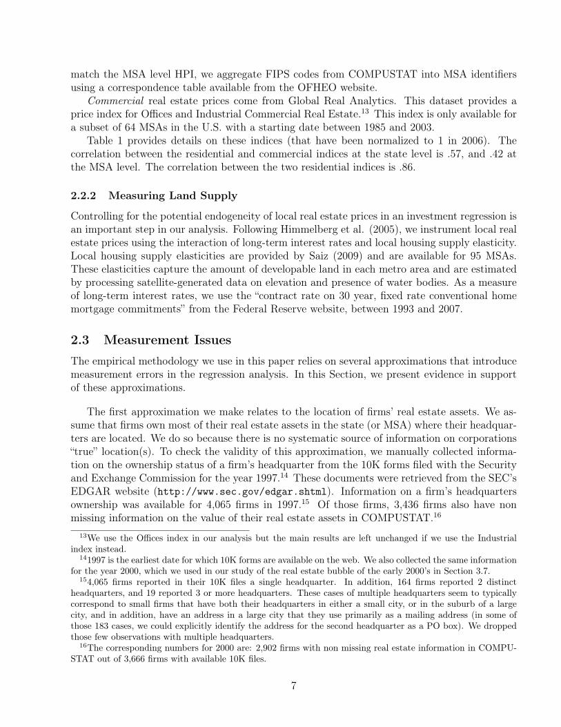
Figure 1 shows the evolution of office prices from 2000 to 2006 depending on the MSA localhousing supply elasticity. It confirms that, while the bubble had a more dramatic impact onresidential prices, it did also affect commercial prices. Low elasticity MSAs experienced a muchlarger increase in office prices (30% increase in 2 years) than high elasticity MSAs. Figure2 implements our methodology looking at total capital expenditures since 2000, normalizedby assets in 2000. In low elasticity MSAs, firms owning their headquarters experienced a 4percentage points higher growth in capital expenditure (blue line) relative to firms rentingtheir headquarters. By contrast, in high elasticities MSAs, there is no statistically significantdifference in the evolution of assets of firms owning their headquarters relative to firms rentingthem (red line). If anything, owners saw a smaller increase in capital expenditure than renters(by about 2 percentage points). Figure 3 leads to similar conclusions on long-term debt: firmsowning their headquarters in low elasticity MSAs took advantage of the real estate price bubbleto increase their stock of debt relative to firms in similar MSAs but renting headquarters andrelative to MSAs where the bubble did not have a large impact on office prices.
Table 10 confirms these graphical evidence using firm-level regressions. We adopt a standardlong-run difference-in-difference strategy and estimate the following equation:
CAPEX00−06im
Assets00im
= αm + β∆(Office Price)00−06
m
Office Price00m
×Headquartersi + γ∆(Office Price)00−06
m
Office Price00m
+ εim (5)
where CAPEX00−06im
Assets00im
is the sum, for firm i, of capital expenditures from 2000 to 2006, normalized
by 2000’s assets. ∆(Office Price)00−06m
Office Prices00m
is, for MSA m, the cumulative office price growth from 2000to 2006. Finally, Headquartersi is a dummy equal to 1 if firm i owns its headquarters in 2000,as reported in its 10K filings of that year.
18

Column (1) in Table 10 directly estimates equation (5). The results from this dummyspecification using the information from the 10K files are to be compared to Column (8) ofTable 6. The .17 coefficient suggests that in response to a 10% real estate price increase, a firmthat owns its headquarters will increase its investment rate by 1.7 percentage point more thana renting firm. The coefficient obtained through focusing on the 2000s is two times larger thanour previous estimates (and than estimates of Gan, 2007a).
Column (2) replaces the local office price growth by the local housing supply elasticity:this corresponds to the reduced form of an instrumental variable regression where local pricesare instrumented by local housing elasticity. As expected, since the higher the local housingelasticity, the lower the increase in local land prices, we find a negative sign on the interactionbetween housing elasticity and the owner dummy: in MSAs with a high housing elasticity, priceincreases have been moderate, and there is not much difference in the investment of ownerscompared to renters; in MSAs with a low housing elasticity, price increases have been dramatic,and owners increase their investment more than renters
Column (3) augments the previous regression in Column (2) by controlling for initial firmsize. This is natural as there is a fair amount of heterogeneity between firms that own versusrent their headquarters.
Column (4) uses quartiles of local housing supply elasticity instead of the elasticity itself.Finally, Columns (5)-(8) replicate the regressions in Columns (1)-(4), replacing cumulative
investment by cumulative long term debt issues (∆Debt00−06im
Assets00im
) as the dependent variable.Overall, the results in Table 10 confirm the analysis of Figures 2 and 3. Firms owning their
headquarters experienced a significantly larger growth in assets and long-term debt relative torenters, especially so in MSAs where office prices increased a lot, i.e. in MSAs with lower housingsupply elasticity. This effect is monotonic in the local housing supply elasticity.
4 ConclusionWhen the value of a firm’s real estate appreciates by $1, its investment increases by approx-imately $.06. This investment is financed through additional debt issues. The impact of realestate shocks on investment is stronger when estimated on a group of firms which are morelikely to be credit constrained. As we showed in this paper, real estate represents a significantfraction of the assets held on the balance sheet of corporations. As a consequence, one couldexpect the impact of real estate shocks on aggregate investment to be non-trivial. However, thisis not necessarily the case in a world where responses to balance sheet shocks are heterogeneous.In particular, small firms respond more than large firms, which attenuates the aggregate impactof credit constraints. Understanding how one can go from the micro estimates we offer in thispaper to the macro impact of real estate shocks on investment, and therefore on GDP, remainsunclear. We hope to tackle this question in future research.
19

References
Almeida, Heitor, Murillo Campello and Michael S. Weisbach, 2004. “The Cash Flow Sensitivityof Cash,” Journal of Finance, American Finance Association, 59(4):1777-1804.
Barro, Robert J, 1976. “The Loan Market, Collateral, and Rates of Interest,” Journal ofMoney, Credit and Banking, Ohio State University Press, 8(4):439-56.
Benmelech, Efraim, Mark J. Garmaise and Tobias J. Moskowitz, 2005. “Do LiquidationValues Affect Financial Contracts? Evidence from Commercial Loan Contracts and ZoningRegulation,” The Quarterly Journal of Economics, 120(3):1121-1154.
Benmelech, Efraim and Nittai Bergman, 2009. “Collateral Pricing”, Journal of FinancialEconomics, 91(3) 339-360.
Benmelech, Efraim and Nittai Bergman, 2008. “Liquidation Values and the Credibility of Fi-nancial Contract Renegotiation: Evidence from U.S. Airlines,” Quarterly Journal of Economics,123(4): 1635-1677.
Bernanke, Benjamin and Mark Gertler, 1989. “Agency Costs, Net Worth and BusinessFluctuations” American Economic Review, 79(1):14-34.
Bernanke, Benjamin S, 1983. “Nonmonetary Effects of the Financial Crisis in Propagationof the Great Depression,” American Economic Review, 73(3):257-76.
Bertrand, Marianne, Esther Duflo and Sendhil Mullainathan, 2004. “How Much Should WeTrust Difference in Difference Estimators ?”, Quarterly Journal of Economics, 119:249-275
Case, Karl, Quigley, John and Robert Shiller , 2001. “Comparing Wealth Effects: The StockMarket Versus the Housing Market,” NBER Working Paper N.8606.
Cutts, Robert, L., 1990. “Power from the Ground Up: Japan’s Land Bubble”, HarvardBusiness Review, 68:164-72.
Eisfeldt, Andrea, and Adriano Rampini, 2009. “Leasing, Ability to Repossess, and DebtCapacity,” Review of Financial Studies, Vol. 22, Issue 4, pp. 1621-1657.
Gan, Jie, 2007a. “Collateral, Debt Capacity, and Corporate Investment: Evidence from aNatural Experiment”, Journal of Financial Economics, 85:709-734.
Gan, Jie, 2007b. “The Real Effects of Asset Market Bubbles: Loan- and Firm-Level Evidenceof a Lending Channel”, Review of Financial Studies, 20:1941-1973.
Goyal, Vidhan and Takeshi Yamada, 2001. “Asset Price Shocks, Financial Constraints andInvestment: Evidence From Japan,”Journal of Business, 77(1):175-200
Hart, Oliver and John Moore, 1994. “A Theory of Debt Based on the Inalienability of HumanCapital,” The Quarterly Journal of Economics, 109(4):841-79.
Himmelberg, Charles, Christopher Mayer and Todd Sinai, 2005. “Assessing High House
20

Prices: Bubbles, Fundamentals and Misperceptions,” Journal of Economic Perspectives, 19(4):67-92.
Kaplan, Steven N. and Luigi Zingales, 1997. “Do Investment-Cash Flow Sensitivities provideUseful Measures of Financing Constraints?”, The Quarterly Journal of Economics, 112: 169-215.
Kiyotaki, Nobuhiro and Moore, John, 1997. “Credit Cycles”, Journal of Political Economy,105 (2): 211–248.
Mian, Atif and Amir Sufi, 2009. “House Prices, Home Equity-Based Borrowing, and the U.S.Household Leverage Crisis”, Working Paper.
Nelson, Theron R., Thomas Potter and Harold H. Wilde, 1999. “Real Estate Asset onCorporate Balance Sheets,” Journal of Corporate Real Estate, 2(1):29-40.
Peek, Joe and Eric S. Rosengren, 2000. ”Collateral Damage: Effects of the Japanese BankCrisis on Real Activity in the United States,” American Economic Review, 90(1):30-45, March.
Rampini, Adriano, and S. Viswanathan, 2010. “Collateral, Risk Management, and the Dis-tribution of Debt Capacity,” Journal of Finance, 65, 2293-2322..
Rauh, Joshua D., 2006. “Investment and Financing Constraints: Evidence from the Fundingof Corporate Pension Plans,” Journal of Finance, 61(1):33-71.
Saiz, Albert, 2010. “On Local Housing Supply Elasticity”, Quarterly Journal of Economics,125 (3): 1253-1296.
Sufi, Amir, 2009, “Bank Lines of Credit in Corporate Finance: An Empirical Analysis”,Review of Financial Studies, 22(3), 1057-1088.
Stiglitz, Joseph E. and Andrew Weiss, 1981. “Credit Rationing in Markets with ImperfectInformation,” American Economic Review, 71(3):393-410.
Townsend, Robert M. , 1979. “Optimal Contracts and Competitive Markets with CostlyState Verification’,” Journal of Economic Theory, 20:265-293.
21

A Figures and Tables
Figure 1: Relative Evolution of Office Prices (High vs. Low Elasticity MSA, 2000-2006)
.91
1.1
1.2
1.3
1.4
1.5
1.6
MS
A o
ffic
e p
ric
es
2000 2002 2004 2006
year
Low elasticity High Elasticity
Note: This figure shows the average office price index (normalized to 1 in 2000) for MSAs in the bottomquartile of land supply elasticity (“Low Elasticity MSA”) in blue and MSAs in the top quartile of landsupply elasticity (“High Elasticity MSA”) in red.
22
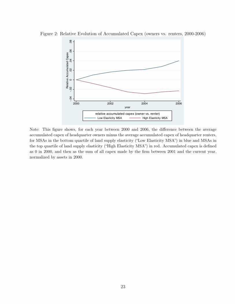
Figure 2: Relative Evolution of Accumulated Capex (owners vs. renters, 2000-2006)
-.0
4-.
02
0.0
2.0
4.0
6.0
8
Re
lativ
e A
cc
um
ula
ted
Ca
pe
x
2000 2002 2004 2006
year
Low Elasticity MSA High Elasticity MSA
relative accumulated capex (owner vs. renter)
Note: This figure shows, for each year between 2000 and 2006, the difference between the averageaccumulated capex of headquarter owners minus the average accumulated capex of headquarter renters,for MSAs in the bottom quartile of land supply elasticity (“Low Elasticity MSA”) in blue and MSAs inthe top quartile of land supply elasticity (“High Elasticity MSA”) in red. Accumulated capex is definedas 0 in 2000, and then as the sum of all capex made by the firm between 2001 and the current year,normalized by assets in 2000.
23
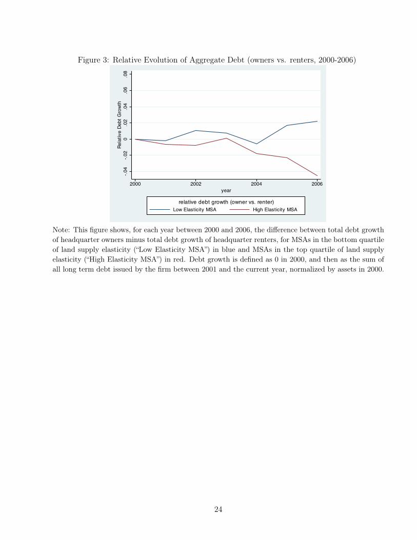
Figure 3: Relative Evolution of Aggregate Debt (owners vs. renters, 2000-2006)
-.0
4-.
02
0.0
2.0
4.0
6.0
8
Re
lativ
e D
eb
t G
row
th
2000 2002 2004 2006
year
Low Elasticity MSA High Elasticity MSA
relative debt growth (owner vs. renter)
Note: This figure shows, for each year between 2000 and 2006, the difference between total debt growthof headquarter owners minus total debt growth of headquarter renters, for MSAs in the bottom quartileof land supply elasticity (“Low Elasticity MSA”) in blue and MSAs in the top quartile of land supplyelasticity (“High Elasticity MSA”) in red. Debt growth is defined as 0 in 2000, and then as the sum ofall long term debt issued by the firm between 2001 and the current year, normalized by assets in 2000.
24
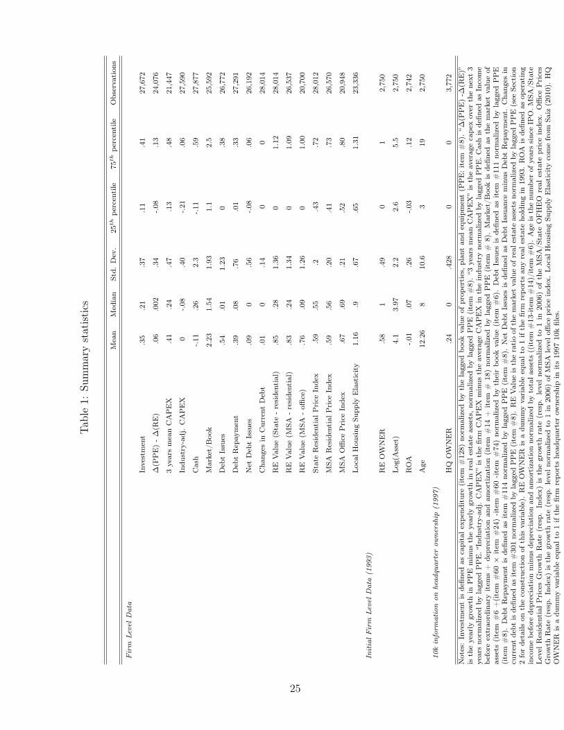
Table1:
Summarystatistics
Mean
Median
Std.
Dev.
25th
percentile
75th
percentile
Observation
s
Fir
mLe
velD
ata
Investment
.35
.21
.37
.11
.41
27,672
∆(P
PE)-
∆(R
E)
.06
.002
.34
-.08
.13
24,076
3yearsmeanCAPEX
.41
.24
.47
.13
.48
21,447
Indu
stry-adj.CAPEX
0-.08
.40
-.21
.06
27,590
Cash
-.11
.26
2.3
-.11
.59
27,877
Market/Boo
k2.23
1.54
1.93
1.1
2.5
25,592
DebtIssues
.54
.01
1.23
0.38
26,772
DebtRepay
ment
.39
.08
.76
.01
.33
27,291
Net
DebtIssues
.09
0.56
-.08
.06
26,192
Cha
nges
inCurrent
Debt
.01
0.14
00
28,014
RE
Value
(State
-residential)
.85
.28
1.36
01.12
28,014
RE
Value
(MSA
-residential)
.83
.24
1.34
01.09
26,537
RE
Value
(MSA
-offi
ce)
.76
.09
1.26
01.00
20,700
StateResidential
Price
Index
.59
.55
.2.43
.72
28,012
MSA
Residential
Price
Index
.59
.56
.20
.41
.73
26,570
MSA
Office
Price
Index
.67
.69
.21
.52
.80
20,948
Local
Hou
sing
Supp
lyElasticity
1.16
.9.67
.65
1.31
23,336
Initia
lFir
mLe
velD
ata
(199
3)
RE
OW
NER
.58
1.49
01
2,750
Log(A
sset)
4.1
3.97
2.2
2.6
5.5
2,750
ROA
-.01
.07
.26
-.03
.12
2,742
Age
12.26
810.6
319
2,750
10k
info
rmat
ion
onhe
adqu
arte
row
ners
hip
(199
7)
HQ
OW
NER
.24
0.428
00
3,772
Notes:Investmentis
defin
edas
capitalexpe
nditure(item
#128)
norm
alized
bythelagged
book
valueof
prop
erties,plan
tan
dequipm
ent(P
PE:item
#8).“∆
(PPE)-∆
(RE)”
istheyearly
grow
thin
PPE
minus
theyearly
grow
thin
real
estate
assets,no
rmalized
bylagged
PPE
(item
#8).“3
yearsmeanCAPEX”is
theaveragecape
xover
thenext
3yearsno
rmalized
bylagged
PPE.“Ind
ustry-ad
j.CAPEX”isthefirm
CAPEX
minus
theaverageCAPEX
intheindu
stry
norm
alized
bylagged
PPE.Cashisdefin
edas
Income
before
extraordinaryitem
s+
depreciation
andam
ortization
(item
#14
+item
#18)no
rmalized
bylagged
PPE
(item
#8).Market/Boo
kis
defin
edas
themarketvalueof
assets
(item
#6+(item
#60×
item
#24)-item
#60
-item
#74
)no
rmalized
bytheirbo
okvalue(item
#6).DebtIssues
isdefin
edas
item
#111no
rmalized
bylagged
PPE
(item
#8).DebtRepaymentis
defin
edas
item
#114no
rmalized
bylagged
PPE
(item
#8).Net
DebtIssues
isdefin
edas
DebtIssuan
ceminus
DebtRepay
ment.
Cha
nges
incurrentdebt
isdefin
edas
item
#301no
rmalized
bylagged
PPE(item
#8).REValue
istheratioof
themarketvalueof
real
estate
assets
norm
alized
bylagg
edPPE(see
Section
2fordetails
ontheconstruction
ofthis
variab
le).
RE
OW
NER
isadu
mmyvariab
leequa
lto
1ifthefirm
repo
rtsan
yreal
estate
holdingin
1993.ROA
isdefin
edas
operating
incomebe
fore
depreciation
minus
depreciation
andam
ortization
norm
alized
bytotala
ssets((item
#13-item
#14)/item
#6).Age
isthenu
mbe
rof
yearssinceIP
O.M
SA/S
tate
Level
Residential
PricesGrowth
Rate(resp.
Index)
isthegrow
thrate
(resp.
levelno
rmalized
to1in
2006)of
theMSA
/State
OFHEO
real
estate
priceindex.
Office
Prices
Growth
Rate(resp.
Index)
isthegrow
thrate
(resp.
levelno
rmalized
to1in
2006)of
MSA
leveloffi
cepriceindex.
Local
Hou
sing
Supp
lyElasticitycomefrom
Saiz
(2010).HQ
OW
NER
isadu
mmyvariab
leequa
lto
1ifthefirm
repo
rtshead
quarterow
nershipin
its1997
10kfiles.
25

Table 2: 10k Headquarter Ownership and Compustat Real Estate Ownership
No HQ ownership in 10k HQ ownership in 10kNo RE in COMPUSTAT 1,572 34> 0 RE in COMPUSTAT 1,024 806
Notes: This table presents the cross-tabulation of headquarter ownership in the 1997 10k file and real estateownership in COMPUSTAT for COMPUSTAT firms in 1997. “> 0 RE in COMPUSTAT” means that the firmreports some real estate ownership in COMPUSTAT in 1997 and “No RE in COMPUSTAT” means that the firmreports no real estate assets in 1997 in COMPUSTAT. “No HQ ownership in 10k” means that the firm reportsthat it leases its headquarter(s) in its 1997 10k file. “HQ ownership in 10k” means that the firm reports that itowns its headquarter(s) in its 1997 10k file.
26
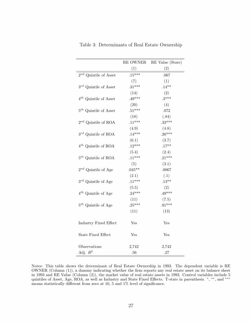
Table 3: Determinants of Real Estate Ownership
RE OWNER RE Value (State)(1) (2)
2nd Quintile of Asset .15*** .067(7) (1)
3rd Quintile of Asset .31*** .14**(14) (2)
4th Quintile of Asset .49*** .3***(20) (4)
5th Quintile of Asset .51*** .072(18) (.84)
2nd Quintile of ROA .11*** .33***(4.9) (4.8)
3rd Quintile of ROA .14*** .26***(6.1) (3.7)
4th Quintile of ROA .12*** .17**(5.4) (2.4)
5th Quintile of ROA .11*** .21***(5) (3.1)
2nd Quintile of Age .045** .0067(2.1) (.1)
3rd Quintile of Age .11*** .13**(5.5) (2)
4th Quintile of Age .24*** .49***(11) (7.5)
5th Quintile of Age .25*** .91***(11) (13)
Industry Fixed Effect Yes Yes
State Fixed Effect Yes Yes
Observations 2,742 2,742Adj. R2 .56 .27
Notes: This table shows the determinant of Real Estate Ownership in 1993. The dependent variable is REOWNER (Column (1)), a dummy indicating whether the firm reports any real estate asset on its balance sheetin 1993 and RE Value (Column (2)), the market value of real estate assets in 1993. Control variables include 5quintiles of Asset, Age, ROA, as well as Industry and State Fixed Effects. T-stats in parenthesis. ∗, ∗∗, and ∗∗∗means statistically different from zero at 10, 5 and 1% level of significance.
27

Table 4: Real Estate Prices and Investment Behavior
Capital Expenditure
(OLS) (OLS) (OLS) (OLS) (OLS) (IV) (OLS) (IV)
(1) (2) (3) (4) (5) (6) (7) (8)
RE Value (State Residential Prices) .077*** .067*** .055***
(15) (13) (12)
RE Value (MSA Residential Prices) .055***
(11)
RE Value (MSA Office Prices) .064*** .065***
(9) (5.5)
RE OWNER × MSA Office Prices .21*** .46***
(3.2) (2.8)
State Residential Prices -.1* -.8** -.38
(-1.7) (-2.1) (-1.1)
MSA Residential Prices -.46
(-1.3)
MSA Office Prices .88 .46 .73 .57
(1.3) (.15) (1.1) (.01)
Cash .017*** .017*** .016*** .016*** .016*** .016***
(6.2) (6.5) (5.5) (3.0) (5.5) (3.1)
Market/Book .062*** .062*** .065*** .064*** .066*** .065***
(18) (19) (18) (9.4) (18) (10.4)
Initial Controls × State Residential Prices No Yes Yes No No No No No
Initial Controls × MSA Residential Prices No No No Yes No No No No
Initial Controls × MSA Office Prices No No No No Yes Yes Yes Yes
Year Fixed Effects Yes Yes Yes Yes Yes Yes Yes Yes
Firm Fixed Effects Yes Yes Yes Yes Yes Yes Yes Yes
Observations 27,670 27,496 24,528 23,222 18,080 17,862 18,313 18,014
Adj. R2 .27 .29 .32 .32 .32 .32 .31 .32
Notes: This table reports the empirical link between the value of real estate assets and investment. The dependent variable iscapital expenditure (item # 128 normalized by lagged item #8). Column (1), (2) and (3) use the state-level residential price index.Column (4) uses MSA-level residential prices, while Column (5),(6) and (7) use MSA-level office prices. Except for column (1),all regressions control for firm-level initial characteristics (5 quintiles of age, asset and ROA as well as 2-digit industry and stateof location) interacted with Real Estate Prices. All regressions, except Column (1) and (2) control for Cash and previous yearMarket/Book. Column (6) and (8) present IV estimates where MSA office prices are instrumented using the interaction of realmortgage rate interacted with the local elasticity of land supply taken from Saiz (2010) (See column (3) in Table 5 for the first stageregressions). All specifications use year and firm fixed effects and cluster observations at the state-year or MSA-year level. In theIV specifications in Columns (6) and (8), standard errors are bootstrapped within MSA-year clusters. T-stats are in parenthesis. ∗,∗∗, and ∗∗∗ means statistically different from zero at 10, 5 and 1% level of significance.
28

Table 5: First-Stage Regression: the Impact of Local Housing Supply Elasticity on HousingPrices
MSA Residential Prices MSA Office Prices(1) (2) (3) (4)
Local Housing Supply Elasticity×Mortgage Rate .028*** .036***(6.3) (5)
First Quartile of Elasticity×Mortgage Rate -.064*** -.066***(-8.9) (-5.1)
Second Quartile of Elasticity×Mortgage Rate -.046*** -.033**(-6) (-2)
Third Quartile of Elasticity×Mortgage Rate -.014** -.0097(-2.2) (-.41)
Year Dummies Yes Yes Yes Yes
MSA Fixed Effect Yes Yes Yes Yes
Observations 1358 1358 804 804Adj. R2 .94 .94 .84 .84
Notes: This table investigates how local housing supply elasticity, as defined by Saiz (2009), affects real estateprices. The dependent variable is the real estate price index, defined at the MSA level – Column (1) and (2) –and the MSA office price index – Column (3) and (4). Column (1) and (3) use directly the local housing supplyelasticity, while Column (2) and (4) use quartiles of the elasticity. All regressions control for year as well as MSAfixed effects and cluster observations at the MSA level. T-stats in parenthesis∗, ∗∗, and ∗∗∗ means statisticallydifferent from zero at 10, 5 and 1% level of significance.
29
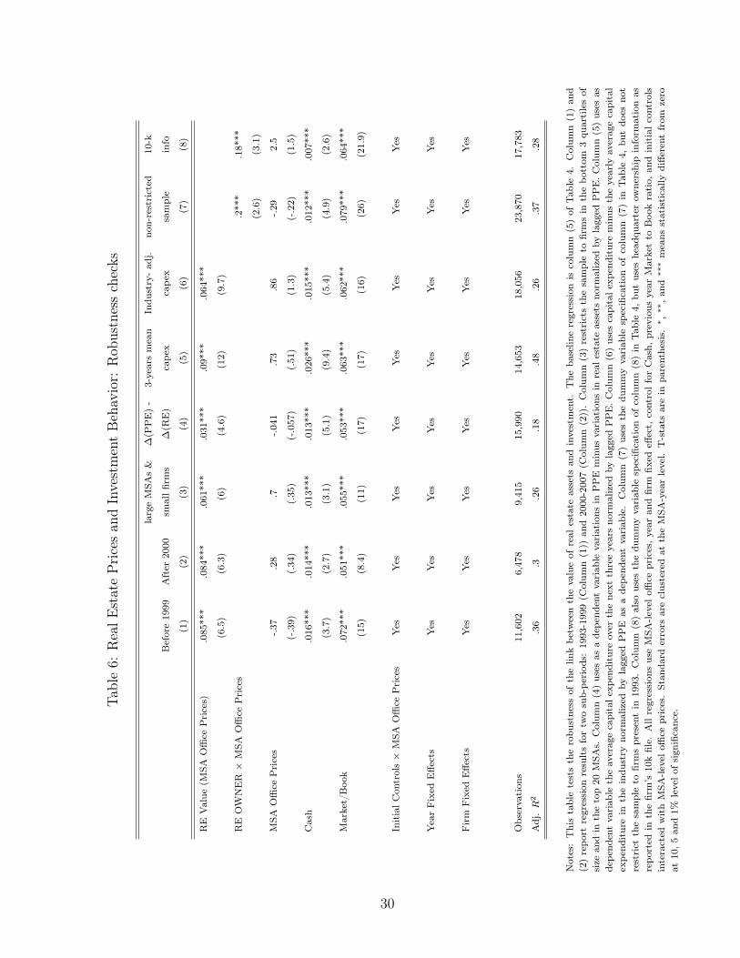
Table6:
RealE
statePricesan
dInvestmentBehav
ior:
Rob
ustnesschecks
largeMSA
s&
∆(P
PE)-
3-yearsmean
Indu
stry-ad
j.no
n-restricted
10-k
Before1999
After
2000
smallfirms
∆(R
E)
cape
xcape
xsample
info
(1)
(2)
(3)
(4)
(5)
(6)
(7)
(8)
RE
Value
(MSA
Office
Prices)
.085***
.084***
.061***
.031***
.09***
.064***
(6.5)
(6.3)
(6)
(4.6)
(12)
(9.7)
RE
OW
NER×
MSA
Office
Prices
.2***
.18***
(2.6)
(3.1)
MSA
Office
Prices
-.37
.28
.7-.041
.73
.86
-.29
2.5
(-.39)
(.34)
(.35)
(-.057)
(.51)
(1.3)
(-.22)
(1.5)
Cash
.016***
.014***
.013***
.013***
.026***
.015***
.012***
.007***
(3.7)
(2.7)
(3.1)
(5.1)
(9.4)
(5.4)
(4.9)
(2.6)
Market/Boo
k.072***
.051***
.055***
.053***
.063***
.062***
.079***
.064***
(15)
(8.4)
(11)
(17)
(17)
(16)
(26)
(21.9)
InitialCon
trols×
MSA
Office
Prices
Yes
Yes
Yes
Yes
Yes
Yes
Yes
Yes
YearFixed
Effe
cts
Yes
Yes
Yes
Yes
Yes
Yes
Yes
Yes
Firm
Fixed
Effe
cts
Yes
Yes
Yes
Yes
Yes
Yes
Yes
Yes
Observation
s11,602
6,478
9,415
15,990
14,653
18,056
23,870
17,783
Adj.
R2
.36
.3.26
.18
.48
.26
.37
.28
Notes:Thistableteststherobu
stness
ofthelin
kbe
tweenthevalueof
real
estate
assets
andinvestment.
The
baselin
eregression
iscolumn(5)of
Tab
le4.
Colum
n(1)an
d(2)repo
rtregression
resultsfortw
osub-pe
riod
s:1993-1999(C
olum
n(1))
and2000-2007(C
olum
n(2)).Colum
n(3)restrictsthesampleto
firmsin
thebo
ttom
3qu
artilesof
size
andin
thetop20
MSA
s.Colum
n(4)uses
asadepe
ndentvariab
levariations
inPPE
minus
variations
inreal
estate
assets
norm
alized
bylagged
PPE.Colum
n(5)uses
asdepe
ndentvariab
letheaveragecapitalexpe
nditureover
thenext
threeyearsno
rmalized
bylagged
PPE.Colum
n(6)uses
capitalexpe
nditureminus
theyearly
averagecapital
expe
nditurein
theindu
stry
norm
alized
bylagged
PPE
asadepe
ndentvariab
le.Colum
n(7)uses
thedu
mmyvariab
lespecification
ofcolumn(7)in
Tab
le4,
butdo
esno
trestrict
thesampleto
firmspresentin
1993.Colum
n(8)also
uses
thedu
mmyvariab
lespecification
ofcolumn(8)in
Tab
le4,
butuses
head
quarterow
nershipinform
ationas
repo
rted
inthefirm’s
10kfile.
Allregression
suseMSA
-level
office
prices,year
andfirm
fixed
effect,
controlforCash,
previous
year
Marketto
Boo
kratio,
andinitialcontrols
interacted
withMSA
-level
office
prices.Stan
dard
errors
areclusteredat
theMSA
-yearlevel.
T-stats
arein
parenthesis.
∗,∗∗,an
d∗∗∗means
statistically
diffe
rent
from
zero
at10,5an
d1%
levelof
sign
ificance.
30

Table7:
RealE
statePricesan
dInvestmentBehav
ior:
“Con
strained”vs.“U
ncon
strained”Firms
Cap
ital
Exp
endit
ure
Payou
tPolicy
Firm
Size
Bon
dRatings
Con
strained
Uncon
strained
Con
strained
Uncon
strained
Con
strained
Uncon
strained
RE
Value
(MSA
Office
Prices)
.087***
.047***
.093***
.045***
.078***
.032***
(7)
(4.3)
(5.9)
(4.6)
(7.2)
(3.7)
MSA
Office
Prices
-.14
-.025
-6.8
-.53
.76
-2.4
(-.057)
(-.022)
(-.71)
(-.48)
(.92)
(-1.2)
Cash
.011***
.04***
.006
.064***
.015***
.043***
(3)
(5.3)
(1.3)
(4.9)
(3.3)
(2.8)
Market/Boo
k.061***
.057***
.05***
.052***
.069***
.061***
(13)
(8.2)
(10)
(6.9)
(12)
(5.5)
InitialC
ontrols×
MSA
Office
Prices
Yes
Yes
Yes
Yes
Yes
Yes
YearFixed
Effe
cts
Yes
Yes
Yes
Yes
Yes
Yes
Firm
Fixed
Effe
cts
Yes
Yes
Yes
Yes
Yes
Yes
Test“C
onst.=
Uncon
st.”
3.04***
2.87***
3.26***
Observation
s9,014
6,160
5,942
4,568
10,584
3,283
Adj.R
2.27
.47
.17
.65
.3.59
Notes:Thistablediffe
rentiatestheresultsof
column(5)in
Tab
le4accordingto
ex-antemeasuresof
credit
constraints.
The
depe
ndentvariab
leis
capitalexpe
nditure(item
#128no
rmalized
bylagged
item
#8).RE
Value
(MSA
Office
Prices)
isthemarketvalueof
real
estate
assets
norm
alized
bylagged
PPE.Allregression
scontrolforfirm-level
initialcharacteristics(5
quintilesof
Age,Asset
andROA
aswellas
initial2-digitindu
stry
andstateof
location
)interacted
withRealEstatePrices,
aswellas
forCashan
dprevious
year
Market/Boo
k.Con
straintcategory
assign
ments
useex
ante
criteria
basedon
firm
dividend
payout
(Colum
n(1)an
d(2)),size
(Colum
n(3)an
d(4))
andbo
ndrating
s(C
olum
n(5)an
d(6)).Test“C
onst.=
Uncon
st.”
isat-test
ofequa
lityof
theREValue
coeffi
cients
betw
eentheconstrainedan
dtheun
constrainedfirms.
Allspecification
suseyear
andfirm
fixed
effectan
dclusterob
servations
attheMSA
-yearlevel.T-stats
inpa
renthesis.
∗,∗∗,an
d∗∗∗means
statistically
diffe
rent
from
zero
at10,5an
d1%
level
ofsign
ificance.
31
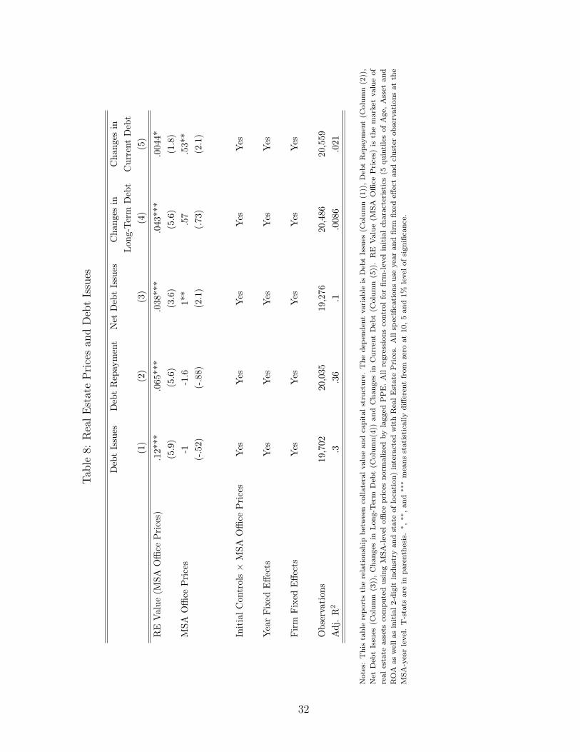
Table8:
RealE
statePricesan
dDebtIssues
DebtIssues
DebtRepayment
Net
DebtIssues
Cha
nges
inCha
nges
inLo
ng-Term
Debt
Current
Debt
(1)
(2)
(3)
(4)
(5)
RE
Value
(MSA
Office
Prices)
.12***
.065***
.038***
.043***
.0044*
(5.9)
(5.6)
(3.6)
(5.6)
(1.8)
MSA
Office
Prices
-1-1.6
1**
.57
.53**
(-.52)
(-.88)
(2.1)
(.73)
(2.1)
InitialC
ontrols×
MSA
Office
Prices
Yes
Yes
Yes
Yes
Yes
YearFixed
Effe
cts
Yes
Yes
Yes
Yes
Yes
Firm
Fixed
Effe
cts
Yes
Yes
Yes
Yes
Yes
Observation
s19,702
20,035
19,276
20,486
20,559
Adj.R
2.3
.36
.1.0086
.021
Notes:Thistablerepo
rtstherelation
ship
betw
eencolla
teralvaluean
dcapitalstructure.
The
depe
ndentvariab
leis
DebtIssues
(Colum
n(1)),DebtRepayment(C
olum
n(2)),
Net
DebtIssues
(Colum
n(3)),Cha
nges
inLon
g-Term
Debt(C
olum
n(4))an
dCha
nges
inCurrent
Debt(C
olum
n(5)).RE
Value
(MSA
Office
Prices)
isthemarketvalueof
real
estate
assets
compu
tedusingMSA
-level
office
prices
norm
alized
bylagged
PPE.Allregression
scontrolforfirm-level
initialcharacteristics(5
quintilesof
Age,Asset
and
ROA
aswellas
initial2-digitindu
stry
andstateof
location
)interacted
withRealEstatePrices.
Allspecification
suseyear
andfirm
fixed
effectan
dclusterob
servations
atthe
MSA
-yearlevel.T-stats
arein
parenthesis.
∗,∗∗,an
d∗∗∗means
statistically
diffe
rent
from
zero
at10,5an
d1%
levelof
sign
ificance.
32
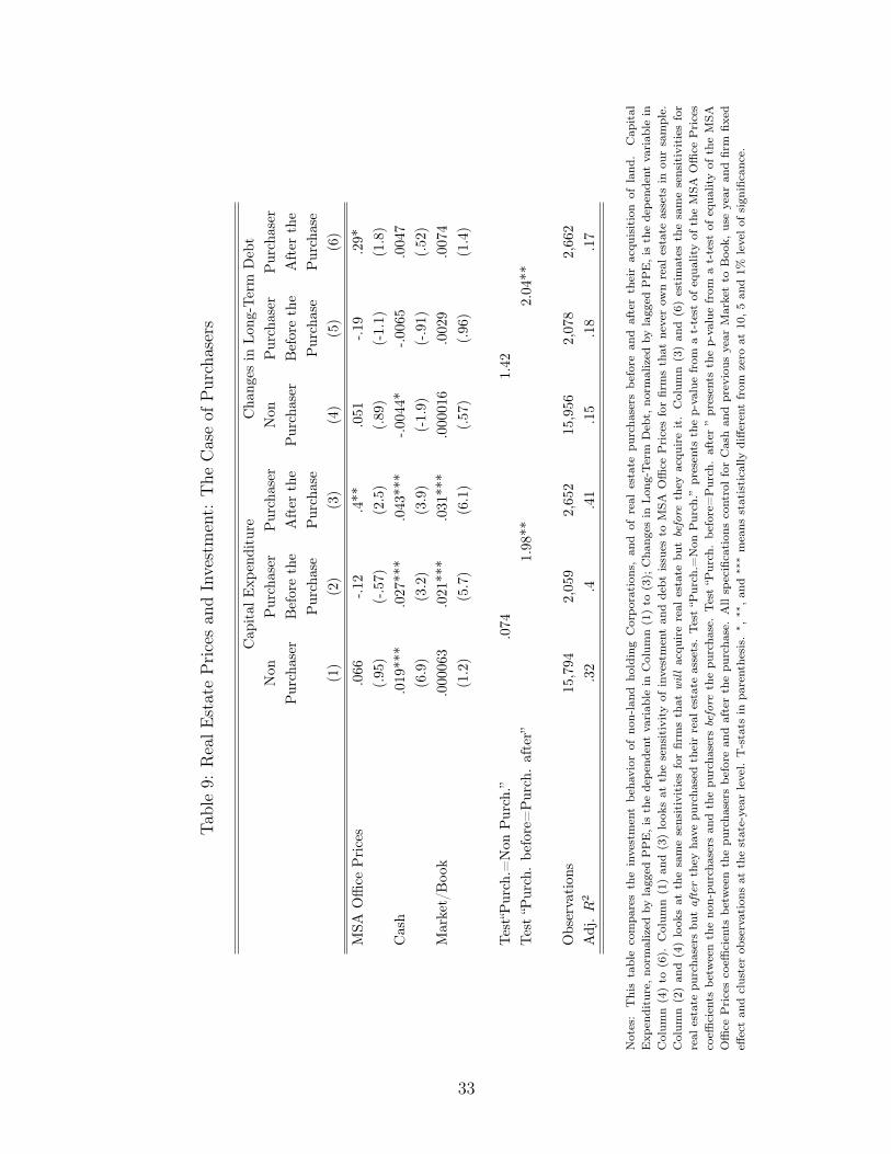
Table9:
RealE
statePricesan
dInvestment:
The
Caseof
Purchasers
Cap
ital
Exp
enditure
Cha
nges
inLo
ng-Term
Debt
Non
Purchaser
Purchaser
Non
Purchaser
Purchaser
Purchaser
Beforethe
After
the
Purchaser
Beforethe
After
the
Purchase
Purchase
Purchase
Purchase
(1)
(2)
(3)
(4)
(5)
(6)
MSA
Office
Prices
.066
-.12
.4**
.051
-.19
.29*
(.95)
(-.57)
(2.5)
(.89)
(-1.1)
(1.8)
Cash
.019***
.027***
.043***
-.0044*
-.0065
.0047
(6.9)
(3.2)
(3.9)
(-1.9)
(-.91)
(.52)
Market/Boo
k.000063
.021***
.031***
.000016
.0029
.0074
(1.2)
(5.7)
(6.1)
(.57)
(.96)
(1.4)
Test“Purch.=
Non
Purch.”
.074
1.42
Test“P
urch.be
fore=Purch.after”
1.98**
2.04**
Observation
s15,794
2,059
2,652
15,956
2,078
2,662
Adj.R
2.32
.4.41
.15
.18
.17
Notes:Thistablecompa
restheinvestmentbe
havior
ofno
n-land
holdingCorpo
ration
s,an
dof
real
estate
purcha
sers
before
and
aftertheiracqu
isition
ofland
.Cap
ital
Exp
enditure,no
rmalized
bylagged
PPE,isthedepe
ndentvariab
lein
Colum
n(1)to
(3);Cha
nges
inLon
g-Term
Debt,no
rmalized
bylagged
PPE,isthedepe
ndentvariab
lein
Colum
n(4)to
(6).
Colum
n(1)an
d(3)look
sat
thesensitivityof
investmentan
ddebt
issues
toMSA
Office
Pricesforfirmsthat
neverow
nreal
estate
assets
inou
rsample.
Colum
n(2)an
d(4)look
sat
thesamesensitivitiesforfirmsthat
willacqu
irereal
estate
but
befo
rethey
acqu
ireit.Colum
n(3)an
d(6)estimates
thesamesensitivitiesfor
real
estate
purcha
sers
butaf
terthey
have
purcha
sedtheirreal
estate
assets.Test“P
urch.=
Non
Purch.”
presents
thep-valuefrom
at-test
ofequa
lityof
theMSA
Office
Prices
coeffi
cients
betw
eentheno
n-pu
rcha
sers
andthepu
rcha
sers
befo
rethepu
rcha
se.Test“P
urch.be
fore=Purch.after”presents
thep-valuefrom
at-test
ofequa
lityof
theMSA
Office
Pricescoeffi
cients
betw
eenthepu
rcha
sers
before
andafterthepu
rcha
se.Allspecification
scontrolforCashan
dprevious
year
Marketto
Boo
k,useyear
andfirm
fixed
effectan
dclusterob
servations
atthestate-year
level.T-stats
inpa
renthesis.
∗,∗∗,an
d∗∗∗means
statistically
diffe
rent
from
zero
at10,5an
d1%
levelof
sign
ificance.
33

Table10
:Headq
uarter
Ownershipan
dtheIm
pact
oftheRealE
stateBub
ble
Accum
ulated
Cap
exCha
nges
intotaldebt
(1)
(2)
(3)
(4)
(5)
(6)
(7)
(8)
Headq
uarter
Owner×
∆(office
prices) 2
000−
2006
.17**
.076*
(2.3)
(1.7)
Headq
uarter
Owner×
Elasticity
-.1***
-.11***
-.048***
-.05
***
(-2.7)
(-2.9)
(-2.7)
(-2.8)
Headq
uarter
Owner×
Second
Qua
rtile
ofElasticity
-.0039
.012
(-.06)
(.37)
Headq
uarter
Owner×
Third
Qua
rtile
ofElasticity
-.02
-.00
0036
(-.32)
(-.00084)
Headq
uarter
Owner×
Fourth
Qua
rtile
ofElasticity
-.12**
-.067**
(-2)
(-2.2)
Elasticity
.078***
.086***
.0058
.007
(2.8)
(3.1)
(.7)
(.85)
∆(office
prices) 2
000−
2006
-.023
.034
(-.42)
(1.6)
Second
Qua
rtile
ofElasticity
.01
-.016
(.49)
(-.9)
Third
Qua
rtile
ofElasticity
.047
-.013
(1.5)
(-1.1)
Fourth
Qua
rtile
ofElasticity
.12***
.0093
(2.9)
(.84)
Log(A
ssets 2
000)
-.021***
-.021***
-.0039
-.0037
(-4)
(-4.1)
(-1.3)
(-1.3)
Observation
s1,729
1,828
1,828
1,828
1,805
1,904
1,90
41,904
Adj.R
2.0019
.0089
.021
.02
.0051
.003
.0044
.0051
Notes:Thistableexplores
theim
pact
ofthereal
estate
bubb
lefrom
2000
to2006,depe
ndingon
head
quarterow
nershipas
repo
rted
inthe10kfiles.Colum
n(1)to
(4)use
accumulated
capitalexpe
nditures
norm
alized
byinitialassets
asadepe
ndentvariab
le.Colum
n(5)to
(8)usechan
gesin
totaldebt
norm
alized
byinitialassets
asadepe
ndent
variab
le.Elasticityrefers
tolocalho
usingsupp
lyelasticity
prov
ided
inSa
iz(2010).Observation
sareclusteredat
theMSA
Level.T-stats
arein
parenthesis.
∗,∗∗,an
d∗∗∗
means
statistically
diffe
rent
from
zero
at10,5an
d1%
levelof
sign
ificance.
34


