

1730 RHODE ISLAND AVENUE, NW, SUITE 1100, WASHINGTON, DC 20036T (202) 293-5374 F (202) 293-5377 ! [email protected]
#
##check
Background Document for the Sessions:
Dietary Exposure Evaluation Model (DEEM™)and
DEEM™ Decompositing Procedure and Software
Presented by:Leila M. Barraj, D.Sc.
Barbara J. Petersen, Ph.D.J. Robert Tomerlin, Ph.D.
Adam S. DanielNovigen Sciences, Inc.
1730 Rhode Island Ave., NWWashington, DC 20036
United States Environmental Protection Agency (US EPA)Office of Pesticide Programs
401 M Street, SWWashington, DC 20460
Presented to:FIFRA Scientific Advisory Panel (SAP)
Arlington, Virginia
February 29 – March 3, 2000
NSI

Presented by Novigen Sciences, Inc. – Page 1
Table of Contents
1. Intended Applications for DEEM™ and Related Software Including CALENDEX™ ______________ 5
2. Background ________________________________________________________________________ 62.1 Dietary Exposure Assessment__________________________________________________________ 62.2 Special Considerations for Multiple Compound Assessments _________________________________ 82.3 Exposure Assessment Models__________________________________________________________ 92.3.1 Point Estimate ______________________________________________________________________ 92.3.2 Simple Distribution __________________________________________________________________ 92.3.3 Probabilistic or Monte Carlo Assessment _________________________________________________ 9
3. Data used in DEEM™_______________________________________________________________ 103.1 “Hard” data _______________________________________________________________________ 103.2 “Soft” data________________________________________________________________________ 113.2.1 Default Processing Factors ___________________________________________________________ 113.2.2 Residue Data ______________________________________________________________________ 133.2.3 Percent Crop Treated Information______________________________________________________ 133.2.4 Toxicity Estimates__________________________________________________________________ 14
4. Modules__________________________________________________________________________ 144.1 Dietary exposure assessment modules __________________________________________________ 144.1.1 Chronic Module ___________________________________________________________________ 144.1.2 Acute Module _____________________________________________________________________ 144.1.3 Sensitivity Analyses ________________________________________________________________ 154.1.3.1 DEEM™ Chronic Module ___________________________________________________________ 154.1.3.2 DEEM™ Acute Module _____________________________________________________________ 164.2 DEEM™ RDFgen™ Module _________________________________________________________ 16
5. Outputs and Algorithms _____________________________________________________________ 175.1 The DEEM™ Chronic Module ________________________________________________________ 175.1.1 Standard populations in the DEEM™ Chronic Module _____________________________________ 185.1.2 DEEM™ Chronic Module Output _____________________________________________________ 185.1.2.1 Default Output_____________________________________________________________________ 185.1.2.2 Sensitivity Analysis Output___________________________________________________________ 185.1.2.3 Residue documentation file___________________________________________________________ 195.1.3 Derivation of estimates of chronic dietary exposures _______________________________________ 195.1.4 Steps in the estimation of the chronic dietary exposures_____________________________________ 205.2 The DEEM™ Acute Dietary Exposure Assessment Module _________________________________ 205.2.1 Populations in the DEEM™ Acute Module ______________________________________________ 205.2.2 DEEM™ Acute Module Outputs ______________________________________________________ 215.2.2.1 Default output _____________________________________________________________________ 215.2.2.2 Plot file ______________________________________________________________________ 215.2.2.3 Sensitivity analysis output____________________________________________________________ 215.2.2.4 Residue documentation file___________________________________________________________ 225.2.3 Steps in the calculation of the acute daily exposure ________________________________________ 225.2.4 Additional description of DEEM™ algorithms____________________________________________ 235.2.4.1 Calculating the daily total exposures for each person-day in the survey_________________________ 245.2.4.2 Calculating the daily mean exposures___________________________________________________ 245.2.4.3 Calculating the interval (bin) limits of the exposure frequency distribution______________________ 255.2.4.4 The algorithm used in the Monte Carlo simulations ________________________________________ 255.3 Algorithms used in the DEEM™ RDFgen™ module_______________________________________ 265.3.1 RDFgen™ outputs__________________________________________________________________ 265.3.2 RDFgen™ functions ________________________________________________________________ 26

Presented by Novigen Sciences, Inc. – Page 2
5.3.2.1 Individual Analyte Mode ____________________________________________________________ 265.3.2.1.1 Percent Crop Treated Adjustment ______________________________________________________ 265.3.2.1.2 Decompositing ____________________________________________________________________ 275.3.2.2 Cumulative Mode __________________________________________________________________ 295.3.2.2.1 Cumulative Percent Crop Treated Adjustment ____________________________________________ 295.3.2.2.2 Cumulative Decompositing___________________________________________________________ 315.3.2.2.3 Cumulative Processing Factor Adjustments and Cumulative Potency Coefficient Adjustments ______ 31
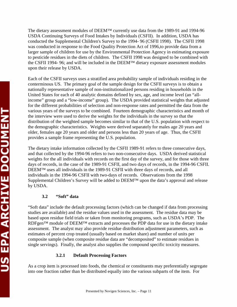
6. Quality Audits and Validation_________________________________________________________ 316.1 DEEM™ Dietary modules ___________________________________________________________ 316.1.1 Validation of the transfer of the data from the USDA CD-ROM to DEEM™ ____________________ 316.1.2 Quality audit of the computational algorithms ____________________________________________ 326.1.2.1 Quality audits performed_____________________________________________________________ 326.1.2.2 Quality audits results________________________________________________________________ 326.1.3 Assessing the impact of the binning procedure on interval estimates ___________________________ 326.1.3.1 Quality audits performed_____________________________________________________________ 326.1.3.2 Quality audits results________________________________________________________________ 336.1.4 Validation of the algorithm used in the Monte Carlo assessment ______________________________ 336.1.4.1 Types of validation analyses __________________________________________________________ 336.1.4.2 Results of the validation analyses ______________________________________________________ 336.1.5 Audit of the randomization algorithms __________________________________________________ 356.1.5.1 Analyses performed ________________________________________________________________ 356.1.5.2 Results of selected analyses __________________________________________________________ 366.2 DEEM™ RDFgen™ Module _________________________________________________________ 376.2.1 Quality audits of the data transfers in the RDFgen™ module_________________________________ 376.2.2 Validation of the decompositing algorithm in RDFgen™ ___________________________________ 386.2.2.1 Validation of the multiple distribution assumption _________________________________________ 386.2.2.2 Validation of the estimation algorithms _________________________________________________ 406.2.2.2.1 Using PDP data ____________________________________________________________________ 406.2.2.2.2 Using hypothetical data______________________________________________________________ 61
7. Other ____________________________________________________________________________ 637.1 Water Consumption ________________________________________________________________ 637.2 Missing body weights _______________________________________________________________ 647.3 Foods with no consumption __________________________________________________________ 64
8.0 References________________________________________________________________________ 65

Presented by Novigen Sciences, Inc. – Page 3
List of Figures
FIGURE 1. COMPONENTS OF A CUMULATIVE RISK ASSESSMENT___________________________ 68
FIGURE 2. DEFAULT OUTPUT OF THE DEEM™ CHRONIC ANALYSIS MODULE _______________ 69
FIGURE 3. DEFAULT OUTPUT OF THE DEEM™ CHRONIC ANALYSIS MODULE _______________ 70
FIGURE 4. DEEM™ CHRONIC MODULE - COMPLETE COMMODITY CONTRIBUTION
ANALYSIS (ALL INFANTS SUBPOPULATION)____________________________________ 71
FIGURE 5. DEEM™ CHRONIC MODULE - CRITICAL COMMODITY CONTRIBUTION
ANALYSIS (ALL INFANTS SUBPOPULATION)____________________________________ 72
FIGURE 6. DEEM™ CHRONIC MODULE - RESIDUE FILE SUMMARY _________________________ 73
FIGURE 7. DEFAULT OUTPUT OF THE DEEM™ ACUTE MODULE ____________________________ 74
FIGURE 8. DEEM™ ACUTE MODULE PLOT FILE ___________________________________________ 75
FIGURE 9. DEEM™ ACUTE MODULE CRITICAL EXPOSRE CONTRIBUTION ANALYSIS_________ 76
FIGURE 10. DEEM™ RESIDUE FILE SUMMARY _____________________________________________ 78

Presented by Novigen Sciences, Inc. – Page 4
List of Appendices
Appendix 1. Listing of Foods, Food Forms, and Crop Groups_______________________________________ 80
Appendix 2. Algorithm Documentation for the DEEM™ Acute and Chronic ProgramModules _____________________________________________________________________ 116

Presented by Novigen Sciences, Inc. – Page 5
The DEEM™ Dietary Exposure Model and Software
The purpose of this paper is to provide comprehensive documentation of the algorithms used bythe Novigen Sciences’ Dietary Exposure and Evaluation Model (DEEM™) to estimate dietaryexposure in order to allow facilitate the peer review of this software by the EPA ScienceAdvisory Panel (SAP). Each of these algorithms has been applied to a wide variety of differentintake estimate problems – ranging from estimating the intake of pesticides to the intake ofnutrients during development of the program. Since its development, various scientists haveused the software for conducting scores of dietary intake assessments. Since the algorithms mustbe evaluated in the context of their intended applications, the paper begins with a brief discussionof those applications. The algorithms themselves are presented in subsequent sections. Thecorresponding computer codes for the computational algorithms are provided in Appendix 2.This paper also includes a discussion of the data that are used by DEEM™. DEEM™ hasundergone extensive QA/QC testing. The results of those tests are summarized for the SAP inthis document. The fidelity of the process used to incorporate the data into DEEM™ has beenverified through testing that is also described in this report. DEEM™ is currently licensed togovernment (US EPA, EPA Canada and the California Department of Pesticide Regulations andto more than 20 other clients). Licensees actively participate in improving the capabilities ofDEEM™ through User group meetings and by providing Novigen examples of analyses andoptions. The software is routinely tested and frequently upgraded through the addition of moreadvanced calculation capabilities and new data bases as they become available. Each newversion of the software undergoes thorough testing including in-house testing and subsequent“beta” testing by users prior to release of software that can be used for analyses conducted underthe requirements of the Good Laboratory Practices (GLP) regulations.
The algorithms in DEEM™ also form the basic platform used for aggregate assessments inCALENDEX™. DEEM™ contains a representative population (e.g., weighted to berepresentative of the entire U.S. population) that provides a sample frame with both demographicinformation and food consumption data.
1. Intended Applications for DEEM™ and Related Software Including CALENDEX™
DEEM™ consists of four software modules: The main DEEM™ module, the Acute analysismodule, the Chronic analysis module, and the RDFgen™ residue distribution module. The mainDEEM™ module is used to create and edit residue files for specific chemical or cumulativeapplications, and to launch the DEEM™ Acute, Chronic, and RDFgen™ modules. TheRDFgen™ module automates single analyte and cumulative residue distribution adjustments andthe creation of summary statistics and Residue Distribution Files based upon USDA PesticideData Program (PDP) monitoring data or user-provided residue data. The Acute analysis andChronic analysis modules provide dietary exposure assessment models based on USDAconsumption data. The DEEM™ software itself is also integrated with CALENDEX™, anaggregate exposure assessment software application focusing on combined dietary andresidential (non-dietary) exposures (Figure 1).

Presented by Novigen Sciences, Inc. – Page 6
The DEEM™ dietary exposure assessment modules can be used to estimate the intake oftoxicants, nutrients, pesticides, food additives, and natural constituents -- in short for anychemical component of food or water. These substances can include inorganic and organicchemicals as well as microorganisms or toxins produced by microorganisms. They can benaturally or synthetically created.
The mere presence of a substance in the food supply does not imply any adverse healthconsequence. In fact some substances of interest are essential nutrients. However, virtually allsubstances are toxic at some dose. Even essential nutrients are toxic, albeit at levels that arehigher than the levels that are essential. Therefore, exposure levels should guide theunderstanding of the significance of the presence of any substance in the diet. Although theinterpretation of the results may be different, the methodologies for estimating exposure aresimilar for toxins, nutrients and microorganisms.
Ingestion will contribute varying amounts to exposure since foods will contain different amountsof each substance on different days. Furthermore, the diets of individuals vary - both betweenindividuals and by the same individual from day to day. DEEM™ is designed to allow the userto tailor the analysis to provide the most appropriate estimates and to allow the user tounderstand the factors that have the most impact on those estimates.
2. Background
2.1 Dietary Exposure Assessment
The goal of dietary exposure assessments is to characterize the exposure of the population ofconcern and to identify the variability of that exposure. Typically, the primary objectives are toestimate the level of ingestion of the substance and to identify the sources of both variability anduncertainty in the estimate. In addition, the exposure assessment can also be useful in aggregateexposure assessments to identify the potential importance of diet relative to other pathways ofexposure and to indicate where consumption of a particular food commodity or other uniquecharacteristic (i.e., age, regional and ethnic preferences), would indicate the potential for uniqueexposure patterns.
To assess the ingestion pathway to total exposure, three types of data are required(1) potential levels in food and water; (2) frequency of occurrence of the substance in food orwater; and (3) amounts of foods that are consumed by the population being evaluated.
The basic dietary exposure model is of the form:
Consumption x Residue = Dietary Exposure
The selection of the most appropriate methodology for an exposure assessment will depend upon(1) the intended application for the exposure assessment, (2) the biological properties of thesubstance, (3) the physical and chemical properties of the substance, (4) the route of entry into

Presented by Novigen Sciences, Inc. – Page 7
food and water, and (5) relative contribution of ingestion to overall exposure. Some of theimportant considerations for each of the five areas are discussed below:
The purpose of the assessment will play a critical role in determining the most desirablemethodology. Different methods will be desirable if the assessment is designed to beconservative (as is often the case for regulatory decision making applications) than when it isdesigned to be as realistic as possible. Some approaches, such as those that assume the foodsupply contains tolerance level residues are designed as “screening” methods. The assumptionthat foods contain residues at the maximum legal limit produces a worst-case intake estimate,often called the theoretical maximum daily intake (TMDI), which dramatically overestimatesexposure. Although it can be very useful for preliminary assessments, for establishing prioritiesor for designing sampling programs is it not as reliable as an estimate of actual intakes.
Screening methods, such as the EPA OPP Tier 1 procedure (see Section 2.3.2), sacrificeaccuracy of estimate for speed, simplicity, and known over-estimation of exposure. In the caseof the evaluation of toxic effects, results that predict that intakes will be less than an acceptableintake level are assumed to mean that exposures will be acceptable. It is further assumed thatthere is no need to expend resources to collect better data or to apply more sophisticatedtechniques in search of greater accuracy.
The length of dosing that is required to elicit a specified biological effect should define the keyexposure assessment parameters. That is, the biological effects that are the result of a single or atmost few doses will be compared to dietary exposure on a single day. Correspondingly, toxiceffects that arise as a result of long term exposure will be compared to average dietary exposures(usually over a year).
Other considerations include whether any breakdown products are of toxicological significanceand the metabolic pathways in plant and animal systems. Potential biological effects must becarefully considered in planning an exposure assessment. Factors of interest include dose-response relationships, the length of exposure required to produce an adverse effect, potentiallysensitive populations, and variability and uncertainty factors.
Often when estimating intake of a substance in food, it is necessary to define or characterize thesubstance in terms of attributes such as structure, volatility, and solubility. Issues that are relatedto the substance’s properties once they are in the food or water include: whether the substancebreaks down during storage, during processing, or during cooking.
The American diet is highly processed. Therefore, for most assessments it will be critical toinclude estimates of the residues in the products as they are consumed (Chin, 1991; Elkins,1991). The DEEM™ software is designed to allow this information to be added as one or moreadjustment factors.
If it is possible to group foods into categories it may be possible for data for one food to beextrapolated to foods for which data are not available. For example, if the levels in oranges wereexpected to be similar to those in grapefruit, it would then be possible to conduct the exposureanalysis for “citrus.” These food categories can then be used to select the most appropriate food

Presented by Novigen Sciences, Inc. – Page 8
consumption data for the assessment. DEEM™ users can group foods by the EPA crop groupingsystem or by defining their own food categories.
2.2 Special Considerations for Multiple Compound Assessments
The method used to estimate dietary exposure to multiple chemicals needs to adjust the detectedresidue levels of each of the chemicals considered, by "relative toxicity factors" that reflect thetoxicity levels of these chemicals relative to a "standard" chemical. A total adjusted residue thenmay be derived for each sample by summing the adjusted residue values corresponding to thatsample. An exposure assessment is then conducted using these total adjusted residues. Theapproach is based on the concepts proposed by the National Academy of Sciences (NAS) for theassessment of joint exposure to organophosphate pesticides, and is similar to that followed by theEPA in the case of dioxin-like compounds. DEEM™ does not specify the procedure forestablishing the relative potency, but once the user has determined the relative potency, DEEM™will adjust the residues accordingly.
Based on our experience in conducting cumulative exposures using DEEM™, there are severalfactors that must be considered in order to estimate reliably the probability of effects fromexposure to multiple chemicals. Some of these include:
" Conduct a realistic treatment of the samples with non-detectable residues to reflect actualpesticide usage practices, including the timing of the pesticide applications, and the potentialusage of multiple pesticides on the same crop. A probabilistic approach that incorporatesinformation about usage practices is recommended.
" Conduct a realistic treatment of the samples with non-detectable residues to reflect thepotential distribution of residue levels below the detection limit. A Monte Carlo approachthat incorporates information about the potential association between the detected levels ofthe various chemicals is recommended.
" Determine consistent procedures for addressing situations where one or more relevantcompounds were not estimated or where there is a correlation between the presence of onecompound and that of another.
" Develop methodology to permit modeling that will include the differences in time forrecovery from potential toxic effects and to account for timing for potential exposure to thepopulation.
" Develop a method for expressing toxicity that is not significantly affected by theexperimental doses that were selected for the toxicological testing.
" Identify a common mechanism of action and use that to determine the toxicity, especially insituations where experimental data show that there are multiple mechanisms of action. Forexample, in the case of organophosphates, some of the chemicals inhibit RBC cholinesteraseat higher doses than they inhibit brain cholinesterase, while the reverse is true for others.

Presented by Novigen Sciences, Inc. – Page 9
" Consider using the dose response patterns in deriving the relative toxicity factors.
2.3 Exposure Assessment Models
There are three general exposure assessment models available in DEEM™: point estimate,simple distribution and probabilistic (Monte Carlo). With appropriate adjustments these modelscan also be used for estimating cumulative exposures. DEEM™ specifically allows the user tofollow the current EPA OPP Tier 1-4 procedures for estimating exposure as described below.
2.3.1 Point Estimate
A point estimate of exposure to a specific chemical by a particular population is a broad estimategenerated using one number to represent concentration of the chemical in each food and onenumber to represent intake of these foods by that population. In estimating chronic exposure, thearithmetic mean of residue concentrations is most commonly used; however, if the distribution ofpesticide concentrations is known to be skewed, use of the median (or 50th percentile)concentration is more appropriate (Mosteller and Tukey, 1977). Typically, the most basicmodels combine data on average intake and average concentration levels of the substance toestimate average exposure.
DEEM™ allows the user to select the most appropriate chemical concentration to be used foreach analysis.
2.3.2 Simple Distribution
Single day or "acute" exposures may be computed using a single estimate of the residueconcentrations and a distribution of food intake data for a single meal or for the day. A simpledistribution of exposure is calculated as follows: a single number chosen to representconcentration of the substance in each of the foods of interest may be applied to a distribution ofintake levels for each food. Typically the residue concentration will be a “worst case” residueand the analysis is thus a conservative or screening type analysis.
Current EPA policy is to utilize a tiered approach in assessing acute dietary exposure. Mostoften the EPA Tier 1 analysis for acute dietary intake utilizes the entire consumption distributionand a single upper-bound residue value (usually the tolerance or highest average field trial(HAFT) residue) for all foods included in the analysis. In the Tier 2 analysis, a single upper-bound residue value is used for those commodities considered to be single serving foods (e.g., araw apple or an orange); mean field trial residues (or residues from monitoring data) are used forprocessed or blended commodities (e.g., grains, oils). (Tiers 3 and 4 are discussed below.)
2.3.3 Probabilistic or Monte Carlo Assessment
Probabilistic or Monte Carlo assessments utilize both the anticipated residue distributions and thedistribution of intake levels. Consumption levels vary both between and among individuals,similarly residue levels present on foods also vary. The variations in the consumption andchemical concentrations in those foods produce potential variations in the resulting exposure

Presented by Novigen Sciences, Inc. – Page 10
distributions. Convolution methods can be used to combine the consumption and residuedistributions. When the number of observations forming the distributions is large, Monte Carlotechniques can be used (National Research Council (NRC), 1993).
EPA’s Tier 3 acute analysis approach incorporates the entire consumption distribution and theentire field trial residue distribution for single serving foods; mean field trial residues or theentire distribution from monitoring programs (under certain conditions) are used forprocessed/blended commodities. The Tier 3 analysis may also incorporate percentages of thecrop that may be treated with the chemical of interest. EPA’s Tier 4 analysis utilizes the entireconsumption distribution and residue distributions from statistically designed market basketsurveys. The EPA’s policy regarding use of residue data in dietary intake assessments has beenevolving in recent months. The DEEM™ software is able to incorporate residue data accordingto the EPA’s developing data utilization policy.
DEEM™ provides the user with the capability to conduct Tier 1-4 analysis whenever theresidue data are available for such analyses. Users can also conduct a combination analysis,using Tier 1 or 2 for some commodities and Tiers 3 and 4 for those where the data permit and/orwhere those commodities contribute sufficiently to the risk to warrant a more extensive analysis.
3. Data used in DEEM™
Data used by the DEEM™ modules are of two types. The first type of data are those supplied byDEEM™ and cannot be changed by the user, although the user can use a subset of these data.We refer to these data as “hard” data. These are the consumption and demographic profiles ofthe individuals in USDA’s consumption surveys and the translation factors that translate foods asconsumed (e.g., pizza) into the corresponding raw agricultural commodities and food forms (e.g.,wheat, tomatoes, etc.). The second type of data are those supplied by DEEM™ but that can bemodified by the user or data that are provided by the user. We refer to these data as “soft” data.These are the default processing factors and the residue data that can be extracted from USDA’sPDP via the DEEM™ RDFgen™ module, and other residue data provided by the user. The useralso provides information, such as: the percent of the crop assumed to be treated with thecompound of interest and the chemical specific toxicity measures. Toxicity measures used byDEEM™ include the NOEL, the Reference Dose (whether acute (ARfD) or chronic (RfD)), andthe population adjusted reference doses (PAD).
3.1 “Hard” data
As described above these are the fixed data that cannot be altered by the user, and refer to theconsumption and demographic data of the individuals in USDA’s consumption surveys and thetranslation factors, including the statistical weights developed by USDA. Translation factorstransform amounts of foods as consumed, e.g., pizza, into the various raw agriculturalcommodities (RACs) and food forms, e.g., wheat; processed tomatoes; etc… Appendix #1 listsall RACs and food forms. Translation factors currently being developed by USDA will beincorporated in DEEM™ when USDA makes them available in the spring of 2000.
Presented by Novigen Sciences, Inc. – Page 11
The dietary assessment modules of DEEM™ currently use data from the 1989-91 and 1994-96USDA Continuing Surveys of Food Intakes by Individuals (CSFII). In addition, USDA hasconducted the Supplemental Children's Survey to the 1994- 96 (CSFII 1998). The CSFII 1998was conducted in response to the Food Quality Protection Act of 1996,to provide data from alarger sample of children for use by the Environmental Protection Agency in estimating exposureto pesticide residues in the diets of children. The CSFII 1998 was designed to be combined withthe CSFII 1994- 96; and will be included in the DEEM™ dietary exposure assessment modulesupon their release by USDA.
Each of the CSFII surveys uses a stratified area probability sample of individuals residing in theconterminous US. The primary goal of the sample design for the CSFII surveys is to obtain anationally representative sample of non-institutionalized persons residing in households in theUnited States for each of 40 analytic domains defined by sex, age, and income level (an “all-income” group and a “low-income” group). The USDA provided statistical weights that adjustedfor the different probabilities of selection and non-response rates and permitted the data from thevarious years of the surveys to be combined. Fourteen demographic characteristics and month ofthe interview were used to derive the weights for the individuals in the survey so that thedistribution of the weighted sample becomes similar to that of the U.S. population with respect tothe demographic characteristics. Weights were derived separately for males age 20 years andolder, females age 20 years and older and persons less than 20 years of age. Thus, the CSFIIprovides a sample frame representing the U.S. population.
The dietary intake information collected by the CSFII 1989-91 refers to three consecutive days,and that collected by the 1994-96 refers to two non-consecutive days. USDA derived statisticalweights for the all individuals with records on the first day of the survey, and for those with threedays of records, in the case of the 1989-91 CSFII, and two days of records, in the 1994-96 CSFII.DEEM™ uses all individuals in the 1989-91 CSFII with three days of records, and allindividuals in the 1994-96 CSFII with two-days of records. Observations from the 1998Supplemental Children’s Survey will be added to DEEM™ upon the data’s approval and releaseby USDA.
3.2 “Soft” data
“Soft data” include the default processing factors (which can be changed if data from processingstudies are available) and the residue values used in the assessment. The residue data may bebased upon residue field trials or taken from monitoring programs, such as USDA’s PDP. TheRDFgen™ module of DEEM™ extracts and processes the PDP data for use in the dietary intakeassessment. The analyst may also provide residue distribution adjustment parameters, such asestimates of percent crop treated (usually based on market share) and number of units percomposite sample (when composite residue data are “decomposited” to estimate residues insingle servings). Finally, the analyst also supplies the compound specific toxicity measures.
3.2.1 Default Processing Factors
As a crop item is processed into foods, the chemical or constituents may preferentially segregateinto one fraction rather than be distributed equally into the various subparts of the item. For

Presented by Novigen Sciences, Inc. – Page 12
example, oil-soluble surface residues may remain in the peel. Thus, the resulting concentrationin the citrus peel may be higher than the concentration in the whole orange. Similarly, theresidue concentration in peeled fruit may be lower than in the whole, unpeeled fruit. To addressthis situation, DEEM™ multiplies each food consumption estimate by a default “adjustmentfactor” designed to allow better matching of the residue data with food consumption data. Forexample, raisin consumption is expressed in terms of consumption of actual raisins. If chemicalresidue measurements were made in fresh grapes instead, an adjustment factor must be applied toaccount for the chemical concentration resulting from water loss. This adjustment factor willcorrectly estimate the potential exposure from the raisins.
Default adjustment factors included in the DEEM software are based on yield tables. Sourcesfor these adjustment factors are USDA Handbook 102 (USDA, 1975) and USDA CommodityMaps (USDA, 1982).
Both of these sources provide information on the quantity of processed foods from a unit amountof whole commodity. The USDA Commodity Maps document specifically lists conversionfactors (measures of the physical transformation of a commodity from farm gate toprocessing/consumption) for many foods. The conversion factor is the ratio of the weight of thecommodity in one form to its weight in another form. The factors reflect gains or losses in acommodity. For example, the conversion factor reported for apple juice is 0.774 pounds perpound of fresh apples, indicating that one pound of apples converts to 0.774 pounds of applejuice. If residue data are available only for the whole apple, this conversion factor may be usedto determine the potential impact on the pesticide residues if treated whole apples are processedto juice. That is, since 1.3 pounds of apples are needed to produce one pound of apple juice, it isassumed that the pesticide level in the RAC apples would concentrate 1.3X in the processed juice(1 ÷ 0.774).
The default adjustment factors in DEEM may be considered worst-case because they almostalways assume concentration of residues in the processed commodity. The only exception to thisis the RAC soybean sprouts for which the default factor is 0.33, suggesting a weight gain (i.e.,reduction in pesticide levels) in the processed commodity. If processing studies have beenconducted, processing factors derived from the experimental data may replace the default factorsincluded in the DEEM™ software.
Conversion information may change over time as a result of the adoption of new technology inboth production and processing as well as variation in the physical properties of commoditiesfrom one crop year to another. In addition, as new products become available in the market, newconversion factors may be warranted.
Processing factors can be applied to an entire food or food form using the Residue File Editor inthe main DEEM™ module. However, when performing cumulative assessments, processingfactors are usually supplied a step earlier in the process, using the Cumulative Mode of theRDFgen™ module to correctly apply distinct coefficients to each analyte included in theassessment prior to combining separate distributions into a cumulative distribution.

Presented by Novigen Sciences, Inc. – Page 13
3.2.2 Residue Data
Different types of residue data can be used by DEEM™. The type of data used depends on thetype of assessment being conducted and on the food or food form it represents. Single pointestimates and/or distributions (whether empirical or parametric) may be used. Single pointestimates are used in chronic dietary exposure assessments, or in screening levels acute dietaryexposure assessments. They can also be used to represent residues in foods that undergo a largedegree of blending. Distributions are generally used in more refined dietary exposureassessments and are used to represent foods where residue levels may vary from unit to unit.
Residue data may be provided by the user or may be obtained from monitoring programs such asthe USDA PDP monitoring data via the RDFgen™ module of DEEM™. The RDFgen™module of DEEM™ automates residue distribution adjustments and the creation of summarystatistics and Residue Distribution Files (hereafter referred to as RDF files) using the RDFgen™pre-extracted PDP data sets or user-supplied data. Using the Residue File Editor, the mean valueof an adjusted residue distribution calculated by RDFgen™ can be entered for a chronic riskassessment, or an RDF file generated by RDFgen™ can be referenced for an acute riskassessment. RDFgen™ can also perform adjustments to the residue levels in order to generatecumulative RDF files. RDFgen™ will allow the user to do these analyses automatically usingthe PDP data for samples that have been tested for multiple analytes or manually using user-supplied data. In both situations, the user determines the appropriate adjustment values to use toreflect differences in potency among the chemicals to be analyzed.
The RDFgen™ pre-extracted PDP data sets, at the time of this writing, contain all of the 1994-1997 PDP data. The pre-extracted data sets were compiled from the raw individual sample andresidue databases distributed by the USDA PDP. The pre-extracted PDP residue data setsaccompanying RDFgen™ begin in 1994, since 1994 was the first year in which the PDP beganusing a standardized data format where all non-detect samples were explicitly presented in thedatabase and LOD values were explicitly given for each sample. Novigen will integrate PDPdata for years after 1997 once USDA release them.
Merits of the PDP pesticide monitoring data for dietary risk assessments include:
" Rigorous statistical design." A large number of samples taken of heavily consumed commodities over multi-year
periods." Sensitive analytical methods." Explicit reporting of all analyzed samples (detects and non-detects)." Good quality assurance." Testing of most samples for multiple analytes, enabling cumulative residue operations.
3.2.3 Percent Crop Treated Information
Agricultural commodities are usually grown in several regions and thus may face different pests.Thus, treatments may vary from region to region. In addition, pesticide treatments are notapplied to the entire crop of a specific agricultural commodity. Thus, DEEM™ allows the user

Presented by Novigen Sciences, Inc. – Page 14
to modify residue estimates to reflect the percentage of a crop that is expected to contain residues(“percent crop treated”). This adjustment can be applied through either an adjustment factorused to multiply an average residue value or through incorporation in the residue distributionused in a DEEM™ acute dietary exposure assessment. The latter can be performedautomatically on a single analyte distribution or a cumulative distribution using the RDFgen™module of DEEM™. The user supplies the percent crop treated information.
3.2.4 Toxicity Estimates
Exposure estimates derived by DEEM™ can be compared to compound specific toxicitymeasures to derive risk estimates. The user provides the toxicity measures to be used in thecomparison. The toxicity measure used by DEEM™ depends on the type of assessment beingconducted.
Estimates of chronic dietary exposures are usually compared to the chronic reference dose(cRfD), chronic NOEL, or the Q1*. DEEM™ allows the user to specify which of these measuresto use, and to specify their values. If the RfD is chosen as a measure of toxicity, risk estimatesare expressed as a percent of the RfD, while selecting the NOEL will produce Margins of Safety(Exposure). Selecting the Q1
* permits the user to determine the probability for increased risk ofcancer associated with the calculated exposure.
Estimates of acute dietary exposures are usually compared to the acute reference dose (ARfD),population adjusted reference dose (PAD) or the acute NOEL. If the ARfD or the PAD arechosen as measures of toxicity, risk estimates are expressed as a percent of the ARfD, or PADwhile selecting the NOEL will produce Margins of Safety (Exposure).
4. Modules
4.1 Dietary exposure assessment modules
4.1.1 Chronic Module
Average chronic exposure is usually estimated on a per-capita consumption basis and iscompared to the measure of biological/toxicological results from life-time animal feeding studiesor other appropriate test results. The DEEM™ Chronic Module uses the point estimate modeldescribed above. The equations are presented in Section 5.1. Exposure and risk estimates arederived for the total US population and 25 subpopulations (26 if using the 1989-91 CSFII data).
4.1.2 Acute Module
Acute dietary exposures are calculated using distributions of daily consumption data. The simpledistribution approach is used in the non-Monte Carlo application of the DEEM™ Acute Module,while the probabilistic methodology is used in the Monte Carlo application of this module. The

Presented by Novigen Sciences, Inc. – Page 15
approach used in the Monte Carlo application of the DEEM™ Acute Module is outlined inSection 5 and in Appendix 2 and follows the method outlined by the NRC (1993). The equationsare presented in Section 5.2.
DEEM™ offers two options for estimating acute daily exposures. The first option (“DailyTotal”) combines the distribution of total daily consumption levels with the distribution ofresidue values. The second option (“Eating Occasion”) combines the consumption levelscorresponding to each eating occasion with the distribution of residues and sums the resultingestimated exposures to produce an estimate of the daily exposures. For example, if an individualreported consuming a given food twice during the day (say 100 gm and 120 gm), the “DailyTotal” option would combine the total daily consumption of that food (220 gm) with a randomlyselected residue value. In contrast, the “Eating Occasion” option would combine the firstamount consumed (100 gm) with a randomly selected residue value, and the second amountconsumed (120 gm) with another (possibly different) randomly selected residue value, andcompute a total daily exposure estimate.
4.1.3 Sensitivity Analyses
4.1.3.1 DEEM™ Chronic Module
The DEEM™ Chronic Module allows the user to conduct sensitivity analyses via the ChronicCommodity Contribution Analysis to assess the relative contribution of all the foods and foodforms included in a particular assessments to the total exposure or risk. It also allows the user todetermine which foods and food forms contribute most to the total dietary exposures of each ofthe subpopulations considered.
Two options are available to use to evaluate the contribution of any individual commodity to theexposure estimate:
" Complete Commodity Analysis
The Complete Commodity Analysis reports the contribution of every commodity to thetotal exposure and expresses the contribution both as mg chemical/kg BW/day and as apercent of the Reference Dose (RfD).
" Critical Commodity Analysis
The Critical Commodity Analysis reports the exposure from those foods, whichcontribute a user-specified proportion of the overall exposure, e.g., 1% of total exposure.The critical commodity listing is expressed as both a percent of the RfD and as a percentof total exposure.

Presented by Novigen Sciences, Inc. – Page 16
4.1.3.2 DEEM™ Acute Module
The DEEM™ Acute Module allows the user to conduct sensitivity analyses, via the AcuteCritical Exposure Contribution (CEC) Analysis to determine which foods contribute most to thetotal exposure of all individuals with exposure levels between user-specified percentiles. Theuser can thus determine whether a particular food, residue level or individual food “drives” theassessment, and whether more than one food contributes to most of the exposure of the selectedindividuals.
The computational algorithms used in the CEC are presented in Section 5.2.3 and Appendix 2.
4.2 DEEM™ RDFgen™ Module
RDFgen™ uses QA’ed sets of spreadsheets containing up-to-date monitoring data from the mostwidely used source, the Pesticide Data Program (PDP) of the U.S. Department of Agriculture(USDA). These sets of spreadsheets are ready for immediate use with RDFgen™, and arereferred to by the following titles: “RDFgen™ pre-extracted PDP data set formatted forRDFgen™ Individual Analyte Mode” and “RDFgen™ pre-extracted PDP data set formatted forRDFgen™ Cumulative Mode.”
Additionally, to allow creation of RDFgen™ Cumulative Mode or Individual Analyte ModePDP residue input spreadsheets filtered for specific sample attributes (such as origin or datecollected), Novigen maintains a pre-extracted data set integrating all PDP sample database andresidue database information, plus the following helpful standardized fields:
" COMMOD_NAM (Translated version of the two-character COMMOD field, includingseparation of processed commodities that share COMMOD code with unprocessedcommodities, such as green beans/processed green beans and peaches/canned peaches).
" FULL_PESTN (Standardized version of two-character PEST_NAME field)." BOOKYEAR (PDP data annual report year to which the record belongs)." YEARY2K (Ensures continued ability to correctly sort and query based on sample date)." DETECT (Y/N field indicating whether sample is a detect or non-detect sample)." ORIGINSTD (Standardized version of ORIGIN field, facilitating separation of domestic
samples, imported samples, and samples of unknown origin).
This series of spreadsheets is referred to as the RDFgen™ full Pre-extracted PDP data set.Creation of RDFgen™ Cumulative or Individual Analyte Mode PDP residue input spreadsheetsor user-defined subsets of the RDFgen™ full Pre-extracted PDP data set is automated by theRDFgen™ Input Generator™ Excel add-in.
RDFgen™ can operate in two primary modes: Individual Analyte Mode and Cumulative Mode.The Individual Analyte mode allows the user to perform the following residue adjustments onany single analyte residue distribution:
" Percent Crop Treated" Decompositing

Presented by Novigen Sciences, Inc. – Page 17
The Cumulative mode allows the user to perform the following residue adjustments on anycombination of compounds, provided those individual samples have been tested for co-incidentresidues:
" Percent Crop Treated" Estimation of concentrations in individual fruits/vegetables based on values in a
composite sample (referred to through this document as “decompositing”)" Relative Potency" Processing Factors
RDFgen™ may be launched from within DEEM™ or used independently.
The RDFgen™ module of DEEM™ accepts as input any residue data spreadsheet that has beenformatted according to a specified format. The user is responsible for the quality andrepresentativeness of the data contained in user developed or modified spreadsheets. In general,Individual Analyte Mode input spreadsheets contain distributions for various commodities testedfor a particular chemical, while Cumulative Mode input spreadsheets generally containdistributions for various chemicals tested on a particular commodity. Cumulative Mode shouldbe used when it is desired to combine residue data from multiple analytes into a singledistribution. Note that RDFgen™ Cumulative Mode will only use samples from the CumulativeMode input spreadsheets that have been tested for all of the analytes that are selected forinclusion. Individual analyte mode should be employed when residue distribution adjustmentsare going to be performed on single analyte’s residue data.
5. Outputs and Algorithms
The computational algorithms and codes used by DEEM™ are presented in Appendix 2. Wedescribe below a representative set of these algorithms.
5.1 The DEEM™ Chronic Module
As discussed earlier, chronic dietary exposures are typically derived as point estimates, usingaverage consumption and residue estimates. The DEEM™ Chronic Module derives estimates ofmean per-capita dietary exposure for a pre-defined set of standard populations, and conductssensitivity analyses by estimating the contribution of the various foods to the total exposure.

Presented by Novigen Sciences, Inc. – Page 18
5.1.1 Standard populations in the DEEM™ Chronic Module
Chronic dietary exposure estimates are derived for the following standard populations:
U.S. Pop - 48 states - all seasons
SeasonalU.S. Population - spring seasonU.S. Population - summer seasonU.S. Population - autumn seasonU.S. Population - winter season
RegionalNortheast regionMidwest regionSouthern regionWestern regionPacific Region (Used only in CSFII 1989-91analyses)
EthnicHispanicsNon-hispanic whitesNon-hispanic blacksNon-hispanic other than black or white
Age and GenderAll infants (<1 year)Nursing infants (<1 year)Non-nursing infants (<1 year)Children (1-6 years)Children (7-12 years)Females (13+/pregnant/not nursing)Females (13+/nursing)Females (13-19 yrs/not preg. or nursing)Females (20+ years/not preg. or nursing)Females (13-50 years)Males (13-19 years)Males (20+ years)Seniors (55+)
The Chronic module uses a data base of pre-calculated per-capita mean food consumption data(g/kg-bw-day) for each raw agricultural commodity (RAC) and food/food form reported in theCSFII surveys. The user can also estimate the same value for user-defined subpopulations byusing the per-capita mean estimates provided in the DEEM™ acute module.
5.1.2 DEEM™ Chronic Module Output
5.1.2.1 Default Output
The default output of the DEEM™ Chronic Module consists of the per capita exposureestimates, associated margins of exposure, associated percent of the RfD (Figure 2), orassociated risk (Figure 3), depending on which measure of risk is selected, for the US populationand each of the standard subpopulations.
5.1.2.2 Sensitivity Analysis Output
The output of the optional sensitivity analyses includes, in the case of the Complete CommodityContribution, the listing of all the foods included in the assessment together with theircontribution to the total exposure and expresses the contribution both as mg chemical/kg bw/dayand as a percent of the RfD (Figure 4). If the Critical Commodity Contribution is selected, the

Presented by Novigen Sciences, Inc. – Page 19
output consists of a listing of all foods in the assessment which contribute a user-specifiedproportion of the overall exposure, e.g., 1% of total exposure. The critical commodity listing isexpressed as both a percent of the RfD and as a percent of total exposure (Figure 5).
5.1.2.3 Residue documentation file
In addition, DEEM™ produces a file listing the residue data used in the assessment, anddocumenting the options selected in the assessment, e.g., processing factors and whether percentcrop treated information was used and at what levels (Figure 6).
5.1.3 Derivation of estimates of chronic dietary exposures
Mean estimates of consumption are combined with residue data from a DEEM™ residue file todetermine the mean residue intake (in mg/kg-bw-day) for all individuals in the standardpopulations.
To conduct the chronic risk analyses using the DEEM™ software, the user must thus input threetypes of information:
(1) Concentrations of the constituent or chemical in the foods and/or food-forms. Thesecan include a theoretical level such as the tolerance or MRL (maximum residue limit)or a level anticipated to be found in the food of interest.
(2) Toxicological information about the compound that will be used to evaluate thesignificance of the estimates of exposure. These should include a toxicologyendpoint based on chronic (long-term) exposure such as the cancer potency factor(Q1*), Acceptable Daily Intake (ADI), chronic population adjusted dose (cPAD) orother chronic Reference Dose (RfD), and chronic No Observable Effect Level(NOEL).
(3) Adjustment factors to allow the estimation to more accurately reflect likelyexposures. These adjustment factors can include proportion of the crop treated,proportion imported, processing factors, etc.
The Chronic analysis module calculates per capita daily mean exposures, for each of the standardpopulations, by multiplying the pre-calculated mean consumption values by the correspondingresidue amount, applying adjusting factors, if applicable and normalizing the exposure amountsto mg/kg-bw-day units. The resulting estimates are added for all the foods in the assessment:
jjjj
j AFxPFxsiduexMeanateosureEstimChronicExp Re∑= ,
where Meanj,, Residuej,, PFj, and AFj, represent the pre-calculated mean consumption value,residue value, processing factor and percent crop treated adjustment factor associated with the jth
RAC or food form included in the assessment.

Presented by Novigen Sciences, Inc. – Page 20
The per capita exposure means for all the standard population groups are reported directly, alongwith the estimate of risk based on the chronic toxicology endpoints specified by the user.DEEM™ expresses the expected risk relative to either of the RfD (ADI), cPAD or NOEL(chronic), as selected by the user. It also can express the exposure in relation to the results ofcancer studies. The slope of the dose-response in cancer studies, the Q1*, is used to calculate adose level relevant to a chosen probability value from a cancer study. Specifying the slope of thedose response permits the user determine the probability for increased risk of cancer. In thiscase, the DEEM™ output consists of an estimate of the relationship between the population’sexposure and the probability of occurrence of increased incidence of cancer.
5.1.4 Steps in the estimation of the chronic dietary exposures
The actual source codes for each step in the calculation is presented in Appendix 2.
Step 1. Read in the residue file specific to the analysis1) Read the toxicology endpoints2) Read the residue amounts and conversion factors for each food/food form in the
residue file
Step 2. Read the non-food based (NFB) water consumption means for each standard populationfrom supporting file. Note that NFB water consumption is not reported for eachdrinking occasion, as are other foods, but rather reported as a total daily amount by theindividual and included with the demographic records for that individual.
Step 3. Open files of per capita food consumption means for the appropriate CSFII survey(1989-91 or 1994-96).
Step 4. For each food or food/food form in the residue file (all of which have a default residueamount), retrieve the food consumption record for that food or food/food form from theChronic data base. Multiply the residue amount by the food consumption amount foreach of the populations and sum for this exposure amount separately for eachpopulation. The resulting sums are reported as the total daily exposure for eachpopulation.
Step 5. Calculate the margin of exposure or percent of the cRfD for each population using thetoxicology endpoints and report.
5.2 The DEEM™ Acute Dietary Exposure Assessment Module
5.2.1 Populations in the DEEM™ Acute Module
The DEEM™ Acute Module computes exposure estimates for the total US population and/or anyof the standard subpopulations listed earlier. In addition within each analysis, the user mayspecify up to six additional Custom Populations. Criteria used in the selection of the CustomPopulations include age, gender, geographic region, season, nursing status, race and ethnicity.The USDA food consumption survey from which the CSFII data were developed was designed

Presented by Novigen Sciences, Inc. – Page 21
to provide data representative of the various segments of the US population. Nonetheless, thenumbers of observations for some populations groups, such as nursing infants, is relatively small.In addition, the DEEM™ Acute Module permits the analyst to define custom populations. Caremust be taken not to over-specify a population group for analysis because the number ofobservations available for the group may, likewise, be relatively small. DEEM™ provides tools(such as the Plot File option, see Section 5.2.2.2) for obtaining the detailed information necessaryfor the exposure analyst to evaluate the potential impact of the number of observations upon adietary intake assessment.
5.2.2 DEEM™ Acute Module Outputs
5.2.2.1 Default output
The default output of the DEEM™ Acute Module consists of two summary tables presenting theaverage and standard deviation and selected percentiles of the estimated per-capita and per-userexposure distributions. The summary tables also provide estimates of the associated risks at eachsummary exposure mean and percentile (Figure 7).
Each of the individuals in the 1994-96 CSFII survey contributed up to two days (three days forthe 1989-91 CSFII survey) of consumption data. As mentioned earlier, DEEM™ uses only thoseindividuals with complete consumption records (i.e., two days for the 1994-96 data and threedays for the 1989-91data). The per-capita estimates use all the person-days, while the per-userestimates use the user-days only, that is, the person-days where consumption of the foods ofinterest is reported. The term “person day” is used to describe the food consumption dataprovided by a person during one day of the survey. The term “user day” indicates that at leastone of the foods being considered was consumed by the person on that day.
5.2.2.2 Plot file
In addition, DEEM™ produces a “plot” file consisting of the entire per-user exposuredistribution. The plot file also includes information about the actual (unweighted) and weightednumber of people-days and user-days in the populations considered. The plot file is commadelimited and can be imported in a spreadsheet program for statistical manipulation or to producegraphs (Figure 8).
5.2.2.3 Sensitivity analysis output
In addition to a listing of the analysis parameters (e.g., residue file used, population considered,selected percentiles, minimum contribution), the output of the optional sensitivity analysis, theCritical Exposure Contribution (CEC) analysis, includes the number of records in the selectedrange and a listing of the foods and foodforms and their contributions to the total exposure (indecreasing order of importance). It also lists the records in the selected range, including selecteddemographic characteristics, foods contributing to the exposure, consumption level of thesefoods, residue level, associated exposures, total exposure, and percent of the total daily exposureattributable to the specific foods (Figure 9).

Presented by Novigen Sciences, Inc. – Page 22
5.2.2.4 Residue documentation file
DEEM™ also produces a file listing the residue data used in the assessment and processingvalues used (Figure 10).
5.2.3 Steps in the calculation of the acute daily exposure
There are 10 main steps in the acute analysis calculations. The detailed codes and algorithmscorresponding to each step are presented in Appendix 2.
Step 1. Read in the residue file to be used in this analysis.
Step 2. For any RAC without food forms, convert RACs to their constituent food forms,applying the residue information and adjustment factors to each food form as specifiedfor the RAC itself.
Step 3. (for the Monte Carlo analyses using RDF files) Preprocess all residue distribution files(RDF) declared in the current residue file and save results to two temporary files. Thefirst file contains summary statistics for each RDF file, including the number ofdeclared zeroes, the number of declared LODs (limit of detection), the LOD residuevalue, the number of specified residue values, and a location variable showing thestarting address of its corresponding list of specified residue values in the second file.The second file contains a vector of the individually specified residue values for all ofthe RDF files declared in the residue file.
Step 4. (for the Monte Carlo analyses only) Compute the approximate mean values for eachresidue distribution, the cumulative probability of use for the residue distributionfunctions and the weighted mean for each food/food form and the approximate meanexposure (used to define the interval limits of the exposure distribution).
Step 5. Compute the FFFactor! array of preliminary exposure calculations for each food/foodform having a defined residue in the current residue file. If the Monte Carlo analysis(MCA) is not used, or there is no RDL pointer for the food/food form, then theFFFactor! is the residue amount, multiplied by the adjustment factors. If MCA is usedand one or more RDL pointers are used for any given food/food form, then theexposure represents the adjustment factors only; the residue amount must bedetermined probabilistically from the appropriate residue distribution function. If afood/food form is not included in the residue file, then FFFactor! = 0 for that RAC orfood form.
Step 6. Initial pass through the entire food consumption database to compute the approximatemean daily exposure for users (participants who consume at least one of the food/foodforms in the residue file) in each population group specified when setting up theanalysis. These means will be used to define the interval limits of the exposuredistribution.

Presented by Novigen Sciences, Inc. – Page 23
Step 7. (only used when generating CEC file) Make a pass through the entire food consumptiondata base with 10 iterations (if MCA) or 1 iteration (if no MCA) to determine theapproximate user exposure at the 95th percentile for each population selected.
Step 8. Calculate the total daily exposure for each individual on each day in the survey andplace this exposure amount into the appropriate interval of the exposure distribution forthe particular population. Also generate the summation variables needed to computemean, standard deviation, and standard error of the mean for each population. If thetotal daily exposure exceeds the preliminary exposure estimate at the 95th percentile, asdetermined in step 7, save a record of this individual’s demographic variables (age, sex,body weight) and daily exposure amount, along with a list of the food/food forms eatenthat contribute to this exposure amount, including their consumption amount, residueamount, and adjustment factors. Individual foods/food forms are only included in thislist if their percentage contribution to the total daily exposure exceeds the percentagelevel specified by the user (“minimum exposure contribution by food”).
Step 9. Call the report subroutine to generate the acute analysis report, which contains user andper capita means, standard deviation, and standard error of the mean, as well asexposure distributions for users and per capita, for all designated populations. For eachpopulation of interest, compute the percent of total person-days in the survey that areuser days (i.e., at least one of the food/food form combinations in the residue file wereeaten)
Step 10. (only used when generating CEC file) Generate the CEC file, refining and sorting thelist of CEC records saved during the current analysis. Read the temporary CEC recordsfile generated during the last pass through the food consumption data. For eachpopulation of interest, find all records in the file and save these to a second file sortedby population type (some records may be included in more than one population). Thenread the records for each population individually from the second file; write each recordfor which total daily exposure falls within the low and high percentile bounds specifiedby the user in this run, to a third file. Count the number of times each food/food form isfound in the records in this subset and sum the exposures for each food/food form.Then divide the sum of exposures for each food/food form by the sum or total dailyexposures in this subset to get the percent contribution by each food/food form towardthe total exposure in the referenced percentile interval. Sort the individual records in thesubset in decreasing order of total daily exposure and print the number of individualrecords specified by the user to the final CEC report, starting with the individual withthe highest exposure. (This is repeated for each population of interest; summaries andrecord listings for each population of interest are included in the same CEC report.)
5.2.4 Additional description of DEEM™ algorithms
The DEEM™ Acute Module combines the food and food form consumption values for eachindividual in the population of interest with the residue value associated with the food or foodform. In the Monte Carlo assessment, if a food or food form is associated with a residue

Presented by Novigen Sciences, Inc. – Page 24
distribution, the food and food form consumption values for each individual in the population ofinterest is combined with a randomly selected value from the distribution of residues.
5.2.4.1 Calculating the daily total exposures for each person-day in the survey
In the “daily total” assessments, the consumption values correspond to the total dailyconsumption of the food or food form. In the “eating occasion” assessment the consumptionvalues correspond to the consumption levels at each eating occasion. The total daily exposureestimate for each individual is obtained by summing the calculated for each food or food formreported consumed during that day and dividing by the persons body weight.
Thus, in the “daily total” assessments, the total daily exposure for the kth individual on ith day ofthe survey is obtained as:
kjj
jikik BWsiduexTCExposureTotalDaily /)Re( ,,, ∑= ,
where TCk,i,j represents the total daily consumption by person k on day i of food or food form j,Residuej represents the residue value associated with the food or food form and BWk representsthe body weight of the kth individual.
In the “eating occasion” assessments, the total daily exposure for the kth individual on ith day ofthe survey is obtained as:
kjlj
jlikl
ik BWsiduexTCExposureTotalDaily /)Re( ,,,,, ∑∑= ,
where TCk,i,l,j represents the consumption by person k on the lth eating occasion reported on day iof food or food form j, Residuel,j represents the residue value associated with the food or foodform and BWk represents the body weight of the kth individual.
5.2.4.2 Calculating the daily mean exposures
The per user daily exposure mean is calculated as:
∑∑∑∑=
=ii K
kk
ik
i
K
kik swswxExposureTotalDailynPerUserMea /
1, ,
where swk represents the statistical weight assigned to the kth individual, and Ki represents thenumber of consumers on day i of the survey.
The per capita daily exposure mean is calculated as:
∑∑∑∑=
=N
kk
ik
i
K
kik swswxExposureTotalDailyeanPerCapitaM
i
/1
, ,
where swk represents the statistical weight assigned to the kth individual, and N represents thenumber of individuals in the population of interest.

Presented by Novigen Sciences, Inc. – Page 25
5.2.4.3 Calculating the interval (bin) limits of the exposurefrequency distribution
In the Monte Carlo mode, the software performs the required number of iterations (typically1,000 iterations) for each user-day. Thus, in the DEEM™ version that uses the 1994-96 CSFII, a1000 iteration analysis for Infants could produce 718,000 observations, while analyses with thesame number of iterations for children 1-6 years or the entire US population could result in up to6,074,000 and 30,606,000 observations, respectively. The software resorts to “binning”, i.e.,summarizing the data in frequency intervals, to simplify the task of storing and sorting theseobservations for subsequent use in deriving the exposure distributions.
The bin widths are defined to be a constant percent of the lower bin limit (namely, 1%). Thisapproach provides a method in which the maximum potential error introduced by binning islimited to a fixed value throughout the entire range of bins and does not result in an inordinatenumber of bins. The potential error for a bin, defined to be the percentage difference betweenthe actual exposure value and the mid-point (or end-point) of the bin in which it is placed is thusat most 0.5% (1%) of the exposure value. For exposures that are larger than the mean exposure,the upper bin size of each bin i, i = 1 to n, can simply be defined as (the mean x 1.01i ). Theprocedure allows for up to n = 1100 bins above the mean. Thus, the upper limit of the lastavailable bin is 56,690 times the per-user mean, which provides assurance that high endconsumption amounts of foods usually eaten in small quantities will not exceed the maximumbin. For exposures less than the mean, the method creates 100 bins, of width equal to
(the mean x 100
i).
5.2.4.4 The algorithm used in the Monte Carlo simulations
The algorithm used in the Monte Carlo assessment for the “daily total” analysis follows theapproach used by the NRC (1993), and includes the following steps:
1. The consumption of food 1 by individual 1 on day 1 of the survey period is multipliedby a randomly selected residue value from the residue distribution for food 1.
2. Step 1 is repeated for all foods identified in the assessment that were consumed by
individual 1 on day 1 of the survey.
3. An estimate of the total exposure for person 1 on day 1 is obtained by summing theexposure estimates for all the foods.
4. Steps 1 to 3 are repeated I times (I is the number of iterations specified by the user),still using the consumption data for person 1 on day 1.
5. The I exposure estimates for person 1 on day 1 are stored as I frequencies in theexposure intervals.

Presented by Novigen Sciences, Inc. – Page 26
6. Steps 1 to 5 are repeated for person 1 on subsequent days of the survey period.
7. Steps 1 to 6 are repeated for all individuals in the sub-population.
8. The frequency distribution of the exposure estimates for all individuals on all days isused to derive the percentile estimates.
The detailed algorithms and source code segments are presented in Appendix 2.
5.3 Algorithms used in the DEEM™ RDFgen™ module
5.3.1 RDFgen™ outputs
RDFgen™ output spreadsheets contain basic data attributes (such as units) and summarystatistics for all distributions in the source data spreadsheet, a summary of user-specifiedparameters for residue distribution adjustments, and a listing of the residue distribution(s) at eachphase of adjustment.
RDFgen™ Individual Analyte Mode output spreadsheets also contain single point estimates tobe used for chronic exposure assessment. RDFgen™ generates individual analyte or cumulativeResidue Distribution Files (RDF) ready for immediate use in the DEEM™ Acute module.
5.3.2 RDFgen™ functions
Primary function of RDFgen™ include: (1) percent crop treated adjustment and (2)decompositing of the residues associated with composite samples to produce single servingresidue distributions. In addition, the Cumulative Mode includes processing factor and toxicityadjustments.
5.3.2.1 Individual Analyte Mode
5.3.2.1.1 Percent Crop Treated Adjustment
Percent crop treated adjustment in the Individual Analyte Mode is performed according toChemSAC guidelines (ChemSAC memo dated 1/25/99, “ChemSAC decision re: calculation ofanticipated residues”). Specifically, for a commodity that is not considered blended, e.g., apples,bananas, etc.:
" The percent of samples with detectable residues (PD) is compared to the percent croptreated (PCT).
" If PD ≥ PCT, then all samples with non-detectable residues (if any) are assumed to benon-treated and are assigned a zero residue value.
" If PD < PCT, then a proportion equal to: (100-PCT)/(100-PD) of the samples with non-detectable residues, is assumed to be non-treated and assigned a value equal to zero. Theremaining samples with non-detectable residues are assumed treated (“implied treated”)

Presented by Novigen Sciences, Inc. – Page 27
and are assigned a value equal to half the limit of detection of all samples with non-detectable residues.
On the other hand, all blended commodity samples (e.g., corn oil) are assumed to containresidues, and thus all samples with non-detectable residues are assigned a value equal to half thelimit of detection of all samples with non-detectable residues. In other words, for blendedcommodity samples, the algorithm described above is applied, but with PCT always set to 100%.
5.3.2.1.2 Decompositing
" Assumptions
Food and agricultural commodity samples collected by monitoring programs or field trials aregenerally analyzed as composite samples. Assessment of the potential acute exposure to aspecific contaminant require information about the distribution of residues in individual units offood for those foods likely to be consumed as “single-serving,” e.g., raw apples, bananas, bakedpotatoes, etc. It thus becomes necessary either to analyze these foods as individual units or,alternatively, to use the information from the distribution of residues in the composite samples to“predict” in the residues of the single units making up each composite sample. The purpose ofdecompositing, then, is to predict single serving residues in the absence of single serving data.
Agricultural commodity samples collected by the USDA PDP are analyzed as compositesamples, one composite per location. The treatment history of the samples collected by the PDPis not available. It thus becomes necessary to make assumptions about the proportion of theindividual samples in each composite that are treated with the compound of interest. Theseassumptions are based on information about sample collection and typical packing and shippingpractices of the agricultural commodities being studied. In the case of the PDP samples, sampleswithin a composite are likely to have come from the same field, or from fields in the sameregion. Since samples grown in the same region are likely to have faced the same climate andpest conditions, the single units within PDP composite samples are likely to share the sametreatment “history.”
Thus, a proportion of the composite samples (equal to PCT) is assumed to have been grown intreated locations. Specifically, as described in the previous section, all composite samples withdetectable residues and a sub-sample of the composite samples with non-detectable residues areassumed to have been grown in treated locations (if applicable). All individual units in each ofthese composite samples are assumed to have been treated. If necessary, and if the required dataare available, the proportion of the composites assumed to have been grown in a specific treatedlocation may be allowed to differ from the national estimate of PCT to reflect regionaldifferences in treatment history and sampling practices.
For each “treated” composite, the distribution of single serving residues making that composite isassumed to follow a lognormal distribution (Ott, 1988).

Presented by Novigen Sciences, Inc. – Page 28
" Parameter estimates
The residue value detected in the composite sample value is used to estimate the mean of thelognormal distribution used to represent the residue distribution of the single serving samplesmaking that particular composite. The approach used to estimate the standard deviation of thelognormal distribution depends on whether additional information is available about the relative
variability, or coefficient of variation, = (mean
deviationstandard) of the single serving residues.
Residue data from field trials are often available and may be used to estimate that relativevariability. If that information is available, the standard deviation of the distribution of singleserving residues in a particular composite is estimated by multiplying the value detected in thecomposite sample by the coefficient of variation. Thus, for each treated composite, n singleserving residues are drawn from a lognormal distribution with the following parameters:
Mean = Composite valueSD(ind) = Composite value x Coefficient of variation1
If no information is available, an estimate of the standard deviation is derived assuming thecomposite samples are “repeated” samples from the same population of residues. Thus, for eachtreated composite, n single serving residues are drawn from a lognormal distribution with thefollowing parameters:
Mean = Composite valueSD(ind) = SD(comp) x √ n
Thus, in this case, the estimate of the standard deviation is derived assuming the standarddeviation of the distribution of residues detected in the composite samples is an estimate of thestandard error of the estimated mean of the individual units. Comparisons of the estimates of thestandard deviations derived under this assumption with estimates of the standard deviationderived from observed single serving residues suggests that this approach may overestimate thevariability in the residue distribution of the individual units.
" Sampling single serving residues
Random samples representing single serving residues for each composite are drawn from each ofthe lognormal distributions. Sampling is performed using Latin Hypercube Sampling.Specifically:
" Each lognormal distribution is divided into n equal probability intervals, where nrepresents the number of single servings per composite.
" A random value is selected within each of these intervals." The average of these n random values is computed and compared to the corresponding
composite value.
1 This approach has been implemented only recently, and requires further testing by the EPA.

Presented by Novigen Sciences, Inc. – Page 29
" If the calculated average is within 5% of the composite value, the n individual unitobservations are saved, and the algorithm moves to the next composite and associatedlognormal distribution.
" If the calculated average is not within 5% of the composite value, the n observations arediscarded, n new observations are drawn, their average is calculated and so on until the5% convergence criteria is met. Note that there is no limit on the number of sets of singleunit residue values generated while attempting to achieve convergence within 5% of thecomposite residue value. Such a limit is not needed because convergence reliably occurswithout requiring excessive numbers of attempts. This is a result of the fact that themean of the lognormal distribution is the composite value itself and because LatinHypercube Sampling is used to sample the single serving values.
" All generated single serving samples are combined in a single distribution.
5.3.2.2 Cumulative Mode
5.3.2.2.1 Cumulative Percent Crop Treated Adjustment
Percent crop treated is performed for each selected analyte based on the user-specified percentcrop treated for each analyte using the same algorithm as in the Individual Analyte Mode, withthe following modifications:
" Where the Individual Analyte Mode Percent Crop Treated algorithm replaces n non-detect residue values with a uniform value equal to ½ of the average of the LOD valuesof the distribution’s non-detect samples (as specified by the aforementioned ChemSACmemo); the Cumulative Mode percent crop treated algorithm replaces the n non-detectresidues with ½ of the individual sample LOD value from n non-detect samples from thedistribution.
" The “Probability of Treatment” algorithm is used to determine a subset of the non-detectsamples from each analyte to randomly select from when assigning implied treated (1/2LOD) residue values. By first assuming independence of pesticide use, the “Probabilityof Treatment” algorithm is able to calculate the expected number of samples that willhave been treated with a particular combination of pesticides using the user-specifiedpercent crop treated value for each analyte. For instance:
Illustration of the “implied treated” assignments
This simplified example includes only two compounds; many compounds may beincluded using RDFgen™, provided that samples exist that have been tested for all of thechemicals included.
# Assume that n=200 samples of a particular crop are available, and that analysis ofeach of these samples for compounds A and B, resulted in a total of 40 detectableresidues for compound A and 35 for Compound B, with the following permutationsof each sample:
5 samples with detectable A and B residues35 samples with detectable A residues, and no detectable B residues

Presented by Novigen Sciences, Inc. – Page 30
Illustration of the “implied treated” assignments (Cont’d)
30 samples with detectable B residues and no detectable A residues130 samples with no-detected A and B residues
# Assume that the market shares of compounds A and B are 25% and 30%,respectively.
# Based on the percent crop treated, we expect 50 samples to have been treated forcompound A (200 X .25) and 60 for compound B (200 X .3). We compare theseexpected values with the number of detectable residues, and find that 5 of thesamples (40-35) with no detected A residues must be assigned ½ LOD A residuevalues, and 5 of the samples (35-30) with no detected B residues must be assigned ½LOD B residue values. Note that if it had turned out that the percentage of sampleswith detectable residue values for either compound exceeded that compound’spercent crop treated, the percent crop treated value for that compound would havebeen adjusted upward correspondingly.
# Under the independence assumption, we would expect:15 samples with detectable A and B residues (200 X .25 X .3)35 samples with detectable A residues, and no detectable B residues
(200 X .25 X (1-.3)45 samples with detectable B residues and no detectable A residues
(200 X .3 X (1 -.25) 105 samples with non-detectable A and B residues (200 X 1-.25) X (1-.3)
# Count the actual number of samples matching each of these permutations in the sourceresidue data for the two compounds.
# Adjust each compound for PCT selecting implied treated samples randomly onlyfrom the subsets of the non-detect samples from each compound that do not cause theactual count of samples matching each possible permutation to exceed the expectedcounts.
Excerpt 1 from RDFgen™ spreadsheet output:
DISTRIBUTION HEADING NUM. OF OBS. NUM. OF DETECTS
Compound A 200 40Compound B 200 35
Excerpt 2 from RDFgen™ spreadsheet output:
Compound A Compound B Probability:Expected # ofsamples matchingpattern:
Initial # ofsamples matchingpattern:
# of samplesmatching patternafter adjusting forPCT:
NT NT 0.525 105 130 105NT T 0.225 45 30 45T NT 0.175 35 35 35T T 0.075 15 5 15

Presented by Novigen Sciences, Inc. – Page 31
5.3.2.2.2 Cumulative Decompositing
Decompositing in the Cumulative Mode is performed in exactly the same manner asdecompositing in the Individual Analyte mode. However, to avoid creating an artificialcorrelation between single serving residues from various compounds, the relationship betweensingle serving data points from the different analytes is maintained, randomizing the sequence ofresidue values within each set of single servings belonging to a particular composite in order toprevent generation of unrealistic cumulative single serving values. For instance, assume theanalysis included 2 compounds and 30 composite samples of 6 single servings each. The 6single serving residues generated for compound A and composite (i) are randomly paired withthe 6 single serving residues generated for compound B and composite (i). Note that the“generated” residues for composites assumed not treated for a particular compound are allzeroes.
5.3.2.2.3 Cumulative Processing Factor Adjustments andCumulative Potency Coefficient Adjustments
All residue values in the distributions for each included analyte are multiplied by the user-specified processing factor and/or potency coefficient before each sample’s composite residuevalue is finally determined by summing the adjusted residue values for each included analyte.By adjusting for processing at this stage, any differences in processing among differentcompounds is maintained.
Enhanced versions of RDFgen™ will also include modified RDF specification allowing thecomponent residues to be specified side by side with the cumulative residues to facilitatechemical-based CEC reporting in DEEM™.
6. Quality Audits and Validation
6.1 DEEM™ Dietary modules
DEEM™ outputs and algorithms have undergone extensive validation and quality audits toverify the data transfer, data manipulation, and calculations.
6.1.1 Validation of the transfer of the data from the USDA CD-ROM toDEEM™
Comparisons of DEEM™ outputs and summary tables prepared by USDA were used to confirmthe data transfer from the USDA CD-ROM to DEEM™. Specifically, unweighted counts ofindividuals in various subpopulations provided by USDA summary tables were compared tocounts in DEEM™ outputs, and confirmed that the transfer was done correctly.

Presented by Novigen Sciences, Inc. – Page 32
6.1.2 Quality audit of the computational algorithms
6.1.2.1 Quality audits performed
Audits of the computational algorithms used in DEEM™ are conducted by comparing DEEM™with estimates derived using spreadsheet calculations. These include the algorithms for derivingthe interval limits, the allocation of the observations to the intervals, the calculation of thevarious statistics, including the means, standard deviations, and percentile estimates.
6.1.2.2 Quality audits results
Consumption data for children ages 1 to 6 years were used to test the algorithms. We showbelow representative examples of these tests. Specifically, we compare the estimates of theweighted percent users, per-user mean, standard deviation and standard error, derived usingDEEM™ and those derived using spreadsheet functions.
" Data used:
Consumption of raw apples (RAC 54), FF11 for children ages 1 to 6 years from 1994-96CSFIINumber of children in the population: 3037, each contributing two days of intake for atotal of 6074 person days.
" Results:
Parameter DEEM™Spreadsheetcalculation
Weighted number of person days 49587812 49587812Weighted number of user days 11996587 11996587Weighted percent user days 24.19% 24.1926%Weighted mean (gm/day) 243.0934 243.093437Weighted standard deviation (gm/day) 201.1288 201.128776Weighted standard error (gm/day)1 5.072802 5.07280232
1 The standard error is calculated using the approach used by Ershow and Cantor (LSRO, 1989).
Thus, estimates derived by DEEM™ and spreadsheet calculations are identical
6.1.3 Assessing the impact of the binning procedure on interval estimates
6.1.3.1 Quality audits performed
Consumption data for children ages 1 to 6 years were used to test the algorithms. Percentileestimates derived using the DEEM™ “binned” distributions were compared to percentileestimates derived using the “unbinned” data and SPSS® “WEIGHT” and “PERCENTILE”functions.

Presented by Novigen Sciences, Inc. – Page 33
6.1.3.2 Quality audits results
We show below results of a representative test.
" Data used:
Consumption of raw apples (RAC 54, FF11) for children ages 1 to 6 years from the 1994-96 CSFIINumber of children in the population: 3037, each contributing two days of intake for atotal of 6074 person days
" Results:
Estimates (gm/kg/day)No binningPercentile
DEEM™SPSS®
10 3.869486 3.852620 6.118532 6.078430 7.808793 7.798740 9.827055 9.784250 11.657370 11.638560 14.595180 14.645770 18.193310 18.235380 23.386380 23.396290 34.089500 34.206995 45.324030 45.5046
97.5 56.054500 56.121499 70.996250 71.5096
99.5 84.019320 84.067899.75 104.679300 105.084799.9 117.245400 117.4737
The percentile estimates are virtually identical.
6.1.4 Validation of the algorithm used in the Monte Carlo assessment
6.1.4.1 Types of validation analyses
Consumption data for children ages 1 to 6 years were used to test the algorithms. Exposuredistributions derived from DEEM™ Monte Carlo acute assessment were compared todistributions derived using commercial Monte Carlo software (Crystal Ball®).
6.1.4.2 Results of the validation analyses
Examples using varying degrees of residue data complexity were used. We present below theresults of two such examples.

Presented by Novigen Sciences, Inc. – Page 34
" Example 1:
" Data used:Consumption of orange juice (RAC 36) for children ages 1 to 6 years from the1994-96 CSFIIResidue data: RDF file (empirical distribution) consisting of 106 data points
" Results:
Estimates (mg/kg/day)Parameter
Crystal Ball® DEEM™Number of iterations 10,000 100
Percentile10 0.000004 0.00000420 0.000009 0.00000930 0.000016 0.00001640 0.000029 0.00003050 0.000057 0.00005760 0.000092 0.00009170 0.000129 0.00012880 0.000183 0.00018390 0.000302 0.00029695 0.000519 0.000519
97.5 0.000953 0.00091299 0.001688 0.001629
99.5 0.002424 0.00227499.75 0.003303 0.00297399.9 0.004111 0.004172
Note that the 100 DEEM™ “iterations” correspond to 607,400 iterations in “traditional”Monte Carlo software since, in DEEM™ 100 iterations are performed using each of the6,074 person-days of intake, while in traditional Monte Carlo software, 100 iterations wouldcorrespond to 100 observations drawn from the intake distributions. Percentile estimatesderived using DEEM™ and CRYSTAL BALL® are virtually identical.
" Example 2:
" Data used:
Consumption: RAC 36 and RAC 52 FF 11 for children ages 1 to 6 years from the1994-94 CSFII. This test provides an evaluation of a relatively complex set of foodconsumption data and a combination of several types of residue data. Such a scenariowould be quite common in an actual dietary intake assessment in which several foodsare consumed, and different types of residue data are available for the different typesof food.

Presented by Novigen Sciences, Inc. – Page 35
Residue data:RAC 36, FF 11: Constant value (0.002)RAC 36, FF 12: Constant value (0.002)RAC 36, FF 31: Mixture: 65% zeroes, and 35% from RDF file with 106observationsRAC 36, FF 41: Constant value (0.002)RAC52, FF11: Mixture: 50% zeroes, and 50% lognormal (0.007, 0.006)
" Results:
Estimates (mg/kg/day)Parameter
Crystal Ball® DEEM™Number of iterations 100,000 500
Percentile10 0.000000 0.00000020 0.000000 0.00000030 0.000000 0.00000040 0.000000 0.00000050 0.000002 0.00000260 0.000004 0.00000470 0.000014 0.00001480 0.000039 0.00003990 0.000103 0.00010495 0.000183 0.000182
97.5 0.000286 0.00028599 0.000599 0.000598
99.5 0.001030 0.00102999.75 0.001629 0.00157999.9 0.002439 0.002416
Percentile estimates derived using DEEM™ and CRYSTAL BALL® are virtually identical.
6.1.5 Audit of the randomization algorithms
6.1.5.1 Analyses performed
Analyses were conducted by Novigen and EPA and confirmed that the estimated exposuredistribution is not affected by:
" the order in which the residue values are listed in the RDF file." the method used to adjust the distribution of residues for percent crop treated." the computer used to run the assessment." whether the assessment was run separately or in a “batch” file." random seed (after allowing for enough iterations).
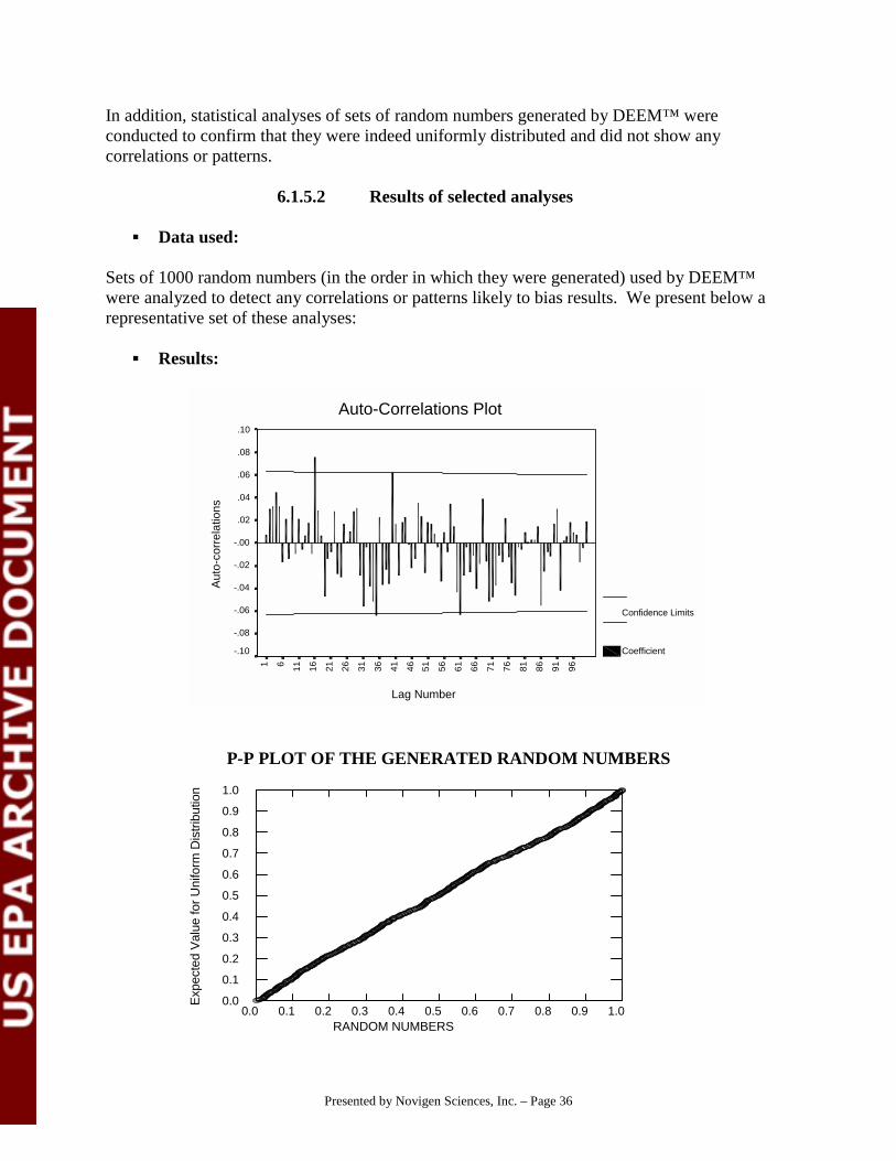
Presented by Novigen Sciences, Inc. – Page 36
In addition, statistical analyses of sets of random numbers generated by DEEM™ wereconducted to confirm that they were indeed uniformly distributed and did not show anycorrelations or patterns.
6.1.5.2 Results of selected analyses
" Data used:
Sets of 1000 random numbers (in the order in which they were generated) used by DEEM™were analyzed to detect any correlations or patterns likely to bias results. We present below arepresentative set of these analyses:
" Results:
Auto-Correlations Plot
Lag Number
96
91
86
81
76
71
66
61
56
51
46
41
36
31
26
21
16
1161
Au
to-c
orr
ela
tion
s
.10
.08
.06
.04
.02
-.00
-.02
-.04
-.06
-.08
-.10
Confidence Limits
Coefficient
P-P PLOT OF THE GENERATED RANDOM NUMBERS
0.0 0.1 0.2 0.3 0.4 0.5 0.6 0.7 0.8 0.9 1.0RANDOM NUMBERS
0.0
0.1
0.2
0.3
0.4
0.5
0.6
0.7
0.8
0.9
1.0
Exp
ecte
d V
alue
for
Uni
form
Dis
trib
utio
n

Presented by Novigen Sciences, Inc. – Page 37
Test of the goodness of fit of the uniform distribution
Test Statistic P-ValueChi-Square (Crystal Ball®) 27.4640 0.4931Kolmogorov-Smirnov (SYSTAT®) 0.025 0.534
The correlations shown in the auto-correlations plot are all negligible (close to zero). Only threeof the 100 estimated coefficients are significantly different from zero (less than the 5% thatwould be expected by chance alone), implying that there are no significant associations betweenthe random numbers. In addition, the P-P plot shows that the random numbers fit a uniformdistribution, as expected if the randomization is functioning correctly.
6.2 DEEM™ RDFgen™ Module
6.2.1 Quality audits of the data transfers in the RDFgen™ module
The Pesticide Data Program information from 1994-1997 was thoroughly checked after it wasreceived from USDA. This included confirming that the records count in the Novigen masterPDP database matched the record count in the official PDP documentation and also spotchecking the contents of the final database against the official PDP annual reports. In addition,every field in the Novigen master PDP database was queried individually and the results werescrutinized for unusual or confusing entries, such as duplicate records, residue values greaterthan 1000 PPM, and samples with non-zero concentrations that were less than the reported LOD.All potential inconsistencies were reported to PDP for confirmation. In every case, the Novigenmaster PDP database proved to be completely consistent with the database utilized by PDP.
The databases utilized by RDFgenTM are derived from the 1994-1997 Novigen master PDPdatabase described above. In order to confirm that the data were extracted properly, detailedqueries were run on the Novigen master PDP database, which generated the number of samplesand the average, minimum, and maximum concentrations for every pesticide and commoditycombination on a year-by-year basis. These results were compared to the statistical outputgenerated during the RDFgenTM extraction process and in all cases the results matched exactly.In addition, all the extracted data were compared result by result to the official PDP annualreports. Again, all potential inconsistencies were reported to PDP for confirmation and onceagain, the Novigen master PDP database proved to be completely consistent with the databaseutilized by PDP.
Presented by Novigen Sciences, Inc. – Page 38
6.2.2 Validation of the decompositing algorithm in RDFgen™
6.2.2.1 Validation of the multiple distribution assumption
" Using PDP data
Observed single serving data from composite samples collected by PDP for two compounds (Aand B) were analyzed to determine the validity of the multiple distribution assumption (Box plotsand Analysis of Variance).
The box plots of the distributions of single serving residues indicate a difference betweencomposites validating the approach of assuming multiple distributions. In addition, the analysisof variance tests conducted indicated a significant difference between the distributions of singleserving residues from different composites (p-values (one-way ANOVA of the log-transformedresidue values) <0.001 for each of the two compounds).
Box Plots of the PDP single serving residues from different composites(Compound A)
Composite
2019181716151413121110987654321
Ob
serv
ed
sin
gle
se
rvin
g r
esi
du
es
.6
.5
.4
.3
.2
.1
0.0

Presented by Novigen Sciences, Inc. – Page 39
Box Plots of the PDP single serving residues from different composites(Compound B)
" Using field trials data
Example 1:
Data on single serving residues from field trials conducted with compound C in 14 differentlocations still show differences (One-way ANOVA of the log-transformed residues, p-value <0.001), even though the trials were conducted under identical conditions.
Box Plots of the single serving residues from different locations(Compound C)
Composite
16151413121110987654321
Ob
serv
ed
sin
gle
se
rvin
g r
esi
du
es
.4
.3
.2
.1
0.0
130130130131130130128130120123117124116120N =
LOCATION
16.0
0
15.0
0
14.0
0
13.0
0
12.0
0
11.0
0
10.0
0
9.0
0
8.0
0
7.0
0
6.0
0
5.0
0
2.0
0
1.0
0
RE
SID
UE
1.4
1.2
1.0
.8
.6
.4
.2
0.0
Presented by Novigen Sciences, Inc. – Page 40
Example 2:
Data on single serving residues and corresponding composites, collected from the SAME fieldwere available. Analysis of variance of the logarithm single serving residues failed to show asignificant composite sample effect, implying that there was no significant difference betweensingle serving residues making composites collected from the same field (One-way ANOVA, p-value = 0.477).
6.2.2.2 Validation of the estimation algorithms
Validation of the algorithms requires comparison of the single serving data generated byRDFgen™ for a given set of composite samples to the actual single serving data that made thesecomposites. Actual residue data of this type are very limited. We used PDP data, field trial data,and simulated data.
6.2.2.2.1 Using PDP data
" Example 1: Compound A – Ten observed single servings per composite
" Data Used:
Single serving analyses for compound A were performed on all single servings from compositeswith quantifiable residues (i.e., > LOQ). Twenty such composite samples and theircorresponding 200 (10 per composite) single serving samples were available. Of the 200 singleserving residues, 29 had trace levels, i.e., residues above the LOD but below the LOQ, and wereassigned a value equal to half the LOQ, and six samples did not have any detectable residues andwere assigned a value equal to half the LOD.
" Results:
Two sets of analyses were conducted. The first assumed that no additional information about therelative variability of the single serving residue distribution was available, while the secondassumed a known coefficient of variation. Typically, the coefficient of variation would beestimated either from field trials or another set of single serving residues, if available. In thisexample, there were no such data, however, to illustrate the impact of using additionalinformation, we estimated the coefficient of variation from each of the 20 sets of single servingresidues, and used the minimum, average and maximum of these 20 estimates (42%, 71% and120%, respectively).
The histograms and summary percentiles indicate that single serving residues generated in theabsence of information (RDFGEN-CLT) show more variability than the observed single servingresidues. Part of this variability is due to the fact that a large proportion of the observed singleserving residues refer to censored values (either at the LOQ or the LOD), while the residuesgenerated by the RDFgen™ approach are not “censored”. Based on the quantile-quantile plotsand the results of the Kolmogorov-Smirnov tests, the generated single serving residues that best“approximate” the observed single serving residues are those generated using an averagecoefficient of variation with RDFgen™. However, based on the results of the Kolmogorov-

Presented by Novigen Sciences, Inc. – Page 41
Smirnov tests, the distribution generated using coefficients of variation of 120% still provides agood fit to the observed data, while the distribution generated using coefficients of variation of42% does not. Note, however, that the quantile-quantile plot of the distribution generated usingcoefficients of variation of 42% indicates a fairly good fit. This apparent contradiction is due tothe fact that the Kolmogorov-Smirnov test focuses on the maximum absolute difference betweenthe two cumulative distributions. Thus, the uncertainty or “imperfect” knowledge of the relativevariability of the single serving residue distributions did not have a significant impact on theresulting generated single serving distributions.

Presented by Novigen Sciences, Inc. – Page 42
HISTOGRAMS OF LOG (RESIDUES)Example 1: PDP - Compound A
20 Composite Samples10 Single Servings Per Composite Sample
log (Observed)
0.0
0 -
.2
5
-.5
0 -
-.2
5
-1.0
0 -
-.7
5
-1.5
0 -
-1
.25
-2.0
0 -
-1
.75
-2.5
0 -
-2
.25
-3.0
0 -
-2
.75
-3.5
0 -
-3
.25
-4.0
0 -
-3
.75
-4.5
0 -
-4
.25
-5.0
0 -
-4
.75
-5.5
0 -
-5
.25
-6.0
0 -
-5
.75
-6.5
0 -
-6
.25
-7.0
0 -
-6
.75
-7.5
0 -
-7
.25
-8.0
0 -
-7
.75
-8.5
0 -
-8
.25
-9.0
0 -
-8
.75
-9.5
0 -
-9
.25
-10.0
0 -
-9.7
5
40
35
30
25
20
15
10
5
0
log(RDFgen-CLT)
0.0
0 -
.2
5
-.5
0 -
-.2
5
-1.0
0 -
-.7
5
-1.5
0 -
-1
.25
-2.0
0 -
-1
.75
-2.5
0 -
-2
.25
-3.0
0 -
-2
.75
-3.5
0 -
-3
.25
-4.0
0 -
-3
.75
-4.5
0 -
-4
.25
-5.0
0 -
-4
.75
-5.5
0 -
-5
.25
-6.0
0 -
-5
.75
-6.5
0 -
-6
.25
-7.0
0 -
-6
.75
-7.5
0 -
-7
.25
-8.0
0 -
-7
.75
-8.5
0 -
-8
.25
-9.0
0 -
-8
.75
-9.5
0 -
-9
.25
-10
.00
- -
9.7
5
40
35
30
25
20
15
10
5
0
log(RDFgen-CV)
0.0
0 -
.2
5
-.5
0 -
-.2
5
-1.0
0 -
-.7
5
-1.5
0 -
-1
.25
-2.0
0 -
-1
.75
-2.5
0 -
-2
.25
-3.0
0 -
-2
.75
-3.5
0 -
-3
.25
-4.0
0 -
-3
.75
-4.5
0 -
-4
.25
-5.0
0 -
-4
.75
-5.5
0 -
-5
.25
-6.0
0 -
-5
.75
-6.5
0 -
-6
.25
-7.0
0 -
-6
.75
-7.5
0 -
-7
.25
-8.0
0 -
-7
.75
-8.5
0 -
-8
.25
-9.0
0 -
-8
.75
-9.5
0 -
-9
.25
-10
.00
- -
9.7
5
40
35
30
25
20
15
10
5
0
LOD LOQ
LOD LOQ
LOD LOQ
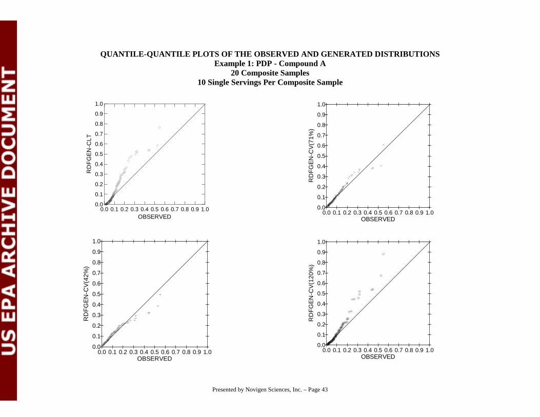
Presented by Novigen Sciences, Inc. – Page 43
QUANTILE-QUANTILE PLOTS OF THE OBSERVED AND GENERATED DISTRIBUTIONSExample 1: PDP - Compound A
20 Composite Samples10 Single Servings Per Composite Sample
0.0 0.1 0.2 0.3 0.4 0.5 0.6 0.7 0.8 0.9 1.0OBSERVED
0.0
0.1
0.2
0.3
0.4
0.5
0.6
0.7
0.8
0.9
1.0
RD
FG
EN
-CL
T
0.0 0.1 0.2 0.3 0.4 0.5 0.6 0.7 0.8 0.9 1.0OBSERVED
0.0
0.1
0.2
0.3
0.4
0.5
0.6
0.7
0.8
0.9
1.0
RD
FG
EN
-CV
(71
%)
0.0 0.1 0.2 0.3 0.4 0.5 0.6 0.7 0.8 0.9 1.0OBSERVED
0.0
0.1
0.2
0.3
0.4
0.5
0.6
0.7
0.8
0.9
1.0
RD
FG
EN
-CV
(42
%)
0.0 0.1 0.2 0.3 0.4 0.5 0.6 0.7 0.8 0.9 1.0OBSERVED
0.0
0.1
0.2
0.3
0.4
0.5
0.6
0.7
0.8
0.9
1.0
RD
FG
EN
-CV
(12
0%
)

Presented by Novigen Sciences, Inc. – Page 44
PERCENTILES OF THE OBSERVED AND GENERATED DISTRIBUTIONSExample 1: PDP - Compound A
20 Composite Samples10 Single Servings Per Composite Sample
Percentile Distributions
200 200 200 200 200
.0800 .0881 .0884 .0884 .0883
.0848 .1337 .0909 .0742 .1233
.0060 .0001 .0050 .0095 .0002
.5500 .7629 .6081 .4932 .8808
.0180 .0012 .0166 .0230 .0106
.0210 .0035 .0241 .0300 .0168
.0310 .0088 .0324 .0384 .0238
.0428 .0173 .0439 .0486 .0333
.0570 .0297 .0587 .0652 .0437
.0690 .0476 .0768 .0852 .0585
.0877 .0812 .0966 .1078 .0838
.1200 .1504 .1323 .1386 .1323
.1600 .2657 .2006 .1889 .2038
.2390 .4310 .3089 .2285 .3278
.3200 .5232 .3706 .2933 .5200
.5292 .5846 .4064 .3837 .6744
.5499 .7620 .6071 .4926 .8798
. . . . .
N
Mean
Std. Deviation
Minimum
Maximum
10.0
20.0
30.0
40.0
50.0
60.0
70.0
80.0
90.0
95.0
97.5
99
99.5
99.9
Percentiles
OBSERVED RDFgenCLT RDFgenCV71 RDFgenCV42 RDFgenCV120

Presented by Novigen Sciences, Inc. – Page 45
Kolmogorov-Smirnov Two Sample Test resultsEXAMPLE 1: PDP - COMPOUND A
20 Composite Samples10 Single Servings Per Composite Sample
Maximum differences for pairs of variables OBSERVED RDFGENCLT RDFGENCV71 RDFGENCV42 RDFGENCV120 OBSERVED 0.000 RDFGENCLT 0.235 0.000 RDFGENCV71 0.070 0.310 0.000 RDFGENCV42 0.140 0.365 0.090 0.000 RDFGENCV120 0.110 0.250 0.140 0.215 0.000
Two-sided probabilities OBSERVED RDFGENCLT RDFGENCV71 RDFGENCV42 RDFGENCV120 OBSERVED . RDFGENCLT 0.000 . RDFGENCV71 0.711 0.000 . RDFGENCV42 0.040 0.000 0.393 . RDFGENCV120 0.178 0.000 0.040 0.000 .

Presented by Novigen Sciences, Inc. – Page 46
Example 2: Compound A – One Observed Single Serving per Composite
" Data Used:
Single serving analyses for compound A were performed on one single serving per composite forall composites. Residue values from 334 composite samples and their corresponding 342 singleserving samples were available. Two single serving analyses were missing, and ten compositesamples had two matching single serving residues. Based on information about the market shareof the compound and the percent samples with detectable residues it was decided to assume thatall samples that had both a non-detectable composite residue and a non-detectable single servingresidue are not treated with the compound of interest. Thus, data from 231 composite samplesand their “corresponding” 238 single serving samples were available for this analysis. Of the238 single serving residues, 33 were below the LOD while 117 were below the LOQ. On theother hand, 11 of the composite samples had residues below the LOD and 94 had residues belowthe LOQ.
The scatter plot (see following Figure) of the observed composite and associated single servingresidues shows a positive association between the two sets of residues. It should be noted thatthe mean and standard deviation of the observed single serving residues (0.0346 ppm and 0.0396ppm) and composite residues (0.0350 ppm and 0.0364 ppm) were very similar. While it is notsurprising that the two averages were similar, it is surprising that the standard deviation of thesingle serving residues is not much larger than that of the composite samples. If the one singleserving residue available for each composite is a true random sample from the single servingsmaking each composite then these results would imply very little variability within composite.However the standard deviation of single serving residues for the same compound, described inExample 1 varied from 0.0114 ppm to 0.174 ppm for the 20 composites (the standard deviationof the entire set of single serving residues, irrespective of composite was 0.0859 ppm).

Presented by Novigen Sciences, Inc. – Page 47
SCATTER PLOT OF THE OBSERVED RESIDUESExample 2: PDP - Compound A
One Observed SS Per Composite Sample
OBSERVED COMPOSITE SAMPLE RESIDUES
.30.25.20.15.10.050.00
OB
SE
RV
ED
SIN
GLE
SE
RV
ING
RE
SID
UE
S.25
.20
.15
.10
.05
0.00

Presented by Novigen Sciences, Inc. – Page 48
" Results:
Two sets of analyses were conducted. The first assumed that no additional information about therelative variability of the single serving residue distribution was available, while the second usedthe average coefficient of variation from the sets of single serving residues described inExample 1.
The single serving residues generated using the average coefficient of variation from the datadescribed in Example 1 show a better fit that those derived in the absence of additionalinformation. However both distributions were significantly different from the observed singleserving residues (Kolmogorov-Smirnov Tests). However, this result is not surprising given thefact that only one observed single serving residue out of 10 is available for each compositesample and the fact that the single serving residue distribution did not show more variability thanthe composite residue distribution (see above discussion).
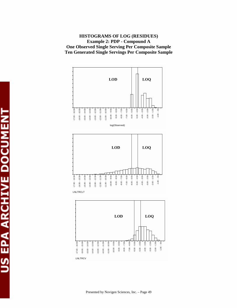
Presented by Novigen Sciences, Inc. – Page 49
HISTOGRAMS OF LOG (RESIDUES)Example 2: PDP - Compound A
One Observed Single Serving Per Composite SampleTen Generated Single Servings Per Composite Sample
log(Observed)
-1.0
0 -
-.5
0
-2.0
0 -
-1
.50
-3.0
0 -
-2
.50
-4.0
0 -
-3
.50
-5.0
0 -
-4
.50
-6.0
0 -
-5
.50
-7.0
0 -
-6
.50
-8.0
0 -
-7
.50
-9.0
0 -
-8
.50
-10
.00
- -
9.5
0
-11
.00
- -
10
.50
-12
.00
- -
11
.50
-13
.00
- -
12
.50
-14
.00
- -
13
.50
-15
.00
- -
14
.50
-16
.00
- -
15
.50
-17
.00
- -
16
.50
LNLTRCLT
-1.0
0 -
-.5
0
-2.0
0 -
-1
.50
-3.0
0 -
-2
.50
-4.0
0 -
-3
.50
-5.0
0 -
-4
.50
-6.0
0 -
-5
.50
-7.0
0 -
-6
.50
-8.0
0 -
-7
.50
-9.0
0 -
-8
.50
-10
.00
- -
9.5
0
-11
.00
- -
10
.50
-12
.00
- -
11
.50
-13
.00
- -
12
.50
-14
.00
- -
13
.50
-15
.00
- -
14
.50
-16
.00
- -
15
.50
-17
.00
- -
16
.50
LNLTRCV
-1.0
0 -
-.5
0
-2.0
0 -
-1
.50
-3.0
0 -
-2
.50
-4.0
0 -
-3
.50
-5.0
0 -
-4
.50
-6.0
0 -
-5
.50
-7.0
0 -
-6
.50
-8.0
0 -
-7
.50
-9.0
0 -
-8
.50
-10
.00
- -
9.5
0
-11
.00
- -
10
.50
-12
.00
- -
11
.50
-13
.00
- -
12
.50
-14
.00
- -
13
.50
-15
.00
- -
14
.50
-16
.00
- -
15
.50
-17
.00
- -
16
.50
LOD LOQ
LOD LOQ
LOD LOQ

Presented by Novigen Sciences, Inc. – Page 50
QUANTILE-QUANTILE PLOTSOF THE OBSERVED AND GENERATED DISTRIBUTIONS
Example 2: PDP - Compound AOne Observed Single Serving Per Composite Sample
Ten Generated Single Servings Per Composite Sample
0.0 0.1 0.2 0.3 0.4 0.5OBSERVED
0.0
0.1
0.2
0.3
0.4
0.5R
DF
GE
N-C
LT
0.0 0.1 0.2 0.3 0.4OBSERVED
0.0
0.1
0.2
0.3
0.4
RD
FG
EN
-CV

Presented by Novigen Sciences, Inc. – Page 51
PERCENTILES OF THE OBSERVED AND GENERATED DISTRIBUTIONSExample 2: PDP - Compound A
One Observed Single Serving Per Composite SampleTen Generated Single Servings Per Composite Sample
Estimated Percentiles
238 2310 2310
.0346 .0350 .0350
.0396 .0678 .0492
.0030 .0000 .0006
.2400 .4753 .6962
.0030 .0001 .0041
.0100 .0004 .0066
.0100 .0011 .0091
.0100 .0025 .0126
.0280 .0106 .0247
.0393 .0237 .0344
.0550 .0539 .0515
.1000 .0988 .0847
.1205 .1836 .1262
.1500 .2583 .1697
.1661 .3438 .2554
.2264 .3777 .3043
. .4496 .4494
N
Mean
Std. Deviation
Minimum
Maximum
10
20
30
40
60
70
80
90
95
97.5
99
99.5
99.9
Percentiles
Observed RDFgenCLT RDFgen-CV
KOLMOGOROV-SMIRNOV TWO SAMPLE TEST RESULTSExample 2: PDP - Compound A
One Observed Single Serving Per Composite SampleTen Generated Single Servings Per Composite Sample
Maximum differences for pairs of groups RDFCLT RDFCV OBSERVED
RDFCLT 0.000 RDFCV 0.376 0.000 OBSERVED 0.451 0.189 0.000
Two-sided probabilities RDFCLT RDFCV OBSERVED RDFCLT . RDFCV 0.000 . OBSERVED 0.000 0.000 .

Presented by Novigen Sciences, Inc. – Page 52
" Example 3: Compound A
" Data Used:
The observed composite and single serving data are the same as those used in Example 2.However, only one of the ten generated single serving samples per composite are used in thisvalidation. Specifically, one single serving value was randomly selected from each set of 10single servings. As in the previous example, the observed single serving values that were belowthe LOD and LOQ were set at half the LOD and half the LOQ in the following summaries.
" Results:
As in the previous example, two sets of analyses were conducted. The first assumed that noadditional information about the relative variability of the single serving residue distribution wasavailable, while the second used the average coefficient of variation from the sets of singleserving residues described in Example 1.
The single serving residues generated using the average coefficient of variation from the datadescribed in Example 1 show a better fit that those derived in the absence of additionalinformation. However both distributions were significantly different from the observed singleserving residues (Kolmogorov-Smirnov Tests). However, as noted earlier, this is not surprising,considering that the observed single serving residues refer to a single observation for the 10apples making the composite and the fact that the single serving residue distribution did notshow more variability than the composite residue distribution.

Presented by Novigen Sciences, Inc. – Page 53
HISTOGRAMS OF THE LOGARITHM OF THE SINGLE SERVING RESIDUESExample 3: Compound A
One observed single serving per compositeOne random generated single serving per composite
log(OBSERVED)
0.0
- .5
-1.0
- -
.5
-2.0
- -
1.5
-3.0
- -
2.5
-4.0
- -
3.5
-5.0
- -
4.5
-6.0
- -
5.5
-7.0
- -
6.5
-8.0
- -
7.5
-9.0
- -
8.5
-10.
0 -
-9.5
-11.
0 -
-10.
5
-12.
0 -
-11.
5
-13.
0 -
-12.
5
-14.
0 -
-13.
5
-15.
0 -
-14.
5
-16.
0 -
-15.
5
-17.
0 -
-16.
5
100
80
60
40
20
0
log(random single serving - RDFgen-CLT)
0.0
- .5
-1.0
- -
.5
-2.0
- -
1.5
-3.0
- -
2.5
-4.0
- -
3.5
-5.0
- -
4.5
-6.0
- -
5.5
-7.0
- -
6.5
-8.0
- -
7.5
-9.0
- -
8.5
-10.
0 -
-9.5
-11.
0 -
-10.
5
-12.
0 -
-11.
5
-13.
0 -
-12.
5
-14.
0 -
-13.
5
-15.
0 -
-14.
5
-16.
0 -
-15.
5
-17.
0 -
-16.
5
100
80
60
40
20
0
log(random single serving - RDFgen-CV)
0.0
- .5
-1.0
- -
.5
-2.0
- -
1.5
-3.0
- -
2.5
-4.0
- -
3.5
-5.0
- -
4.5
-6.0
- -
5.5
-7.0
- -
6.5
-8.0
- -
7.5
-9.0
- -
8.5
-10.
0 -
-9.5
-11.
0 -
-10.
5
-12.
0 -
-11.
5
-13.
0 -
-12.
5
-14.
0 -
-13.
5
-15.
0 -
-14.
5
-16.
0 -
-15.
5
-17.
0 -
-16.
5
100
80
60
40
20
0
LOD LOQ
LOD LOQ
LOD LOQ

Presented by Novigen Sciences, Inc. – Page 54
QUANTILE-QUANTILE PLOTSExample 3: Compound A
One observed single serving per compositeOne random generated single serving per composite
0.0 0.1 0.2 0.3 0.4Observed
0.0
0.1
0.2
0.3
0.4R
ando
m S
S -
RD
Fge
n -
CL
T
0.0 0.1 0.2 0.3 0.4 0.5 0.6 0.7Observed
0.0
0.1
0.2
0.3
0.4
0.5
0.6
0.7
Ra
ndo
m S
S -
RD
Fge
n-
CV

Presented by Novigen Sciences, Inc. – Page 55
PERCENTILE DISTRIBUTIONSExample 3: Compound A
One observed single serving per compositeOne random generated single serving per composite
Percentile Distributions
238 231 231
.0346 .0317 .0368
.0396 .0624 .0615
.0030 .0000 .0032
.0030 .0000 .0035
.0030 .0001 .0041
.0100 .0004 .0069
.0100 .0012 .0102
.0100 .0026 .0127
.0393 .0180 .0316
.0550 .0462 .0508
.1000 .0924 .0928
.1205 .1672 .1286
.1500 .2641 .1705
.1661 .3330 .2635
.2264 .3879 .6282
ValidN
Mean
Std. Deviation
5
6
10
20
30
40
70
80
90
95
97.5
99
99.5
Percentiles
Observed Random-RDFgen-CLT Random-RDFgen-CV
KOLMOGOROV-SMIRNOV TWO SAMPLE TEST RESULTSExample 3: Compound A
One observed single serving per compositeOne random generated single serving per composite
Maximum differences for pairs of groups Observed RDFgen-CLT RDFgen-CV Observed 0.000 RDFgen-CLT 0.277 0.000 RDFgen-CV 0.197 0.394 0.000
Two-sided probabilities Observed RDFgen-CLT RDFgen-CV Observed . RDFfwn-CLT 0.000 . RDFgen-CV 0.000 0.000 .

Presented by Novigen Sciences, Inc. – Page 56
Example 4: Compound B – Ten Observed Single Servings per Composite
" Data Used
Data available:
Data for compound B from composite and matching single serving samples from selectedcomposite samples analyzed by PDP were available. Specifically, 342 composite samples of 10single servings each were available. Twenty of these composite samples had detectablecompound B residues. Single serving residues were available for 16 of these samples. Fourcomposites did not have complete data for their corresponding single serving samples.Specifically, five single serving residues were missing for one composite sample, 2 singleserving residues were missing for two composite samples and one single serving residue wasmissing for one composite sample. Thus, the number of single serving residues available forvalidation was 150.
CID Composite Value Observed Single Serving Residues1
C1 0.15 0.068,0.33,0.17,0.16,0.062,0.057,0.07,0.2,0.12,0.037C2 0.09 0.17,0.16,0.062,nd,0.016,0.09,0.007,0.18,0.055,0.007C3 0.064 nd,nd,nd,0.18,nd,M,M,M,M,M
C4 0.054 M,M,M,M,M,M,M,M,M,M
C5 0.045 0.007,0.007,nd,nd,nd,nd,nd,nd,nd,nd
C6 0.045 0.043,0.056,0.033,0.029,0.028,0.048,0.053,0.038,0.007,0.037
C7 0.044 0.026,0.039,0.032,nd,0.048,nd,0.007,0.055,M,M
C8 0.035 0.057,0.11,0.071,0.047,0.037,0.033,0.021,0.012,0.007,0.013C9 0.03 0.058,nd,0.056,0.007,0.064,0.015,0.007,0.028,0.18,ndC10 0.029 nd,0.061,0.038,0.007,0.061,nd,nd,nd,0.039,M
C11 0.028 0.02,0.094,0.019,0.036,nd,nd,0.019,0.016,0.02,nd
C12 0.023 M,M,M,M,M,M,M,M,M,M
C13 0.007 nd,nd,nd,0.007,nd,nd,nd,nd,nd,0.007
C14 0.007 nd,nd,0.007,0.014,0.028,nd,0.025,0.015,nd,ndC15 0.007 nd,0.035,nd,nd,nd,nd,nd,0.017,M,MC16 0.007 nd,nd,0.007,nd,0.047,nd,nd,nd,0.052,0.007
C17 0.007 nd,nd,nd,0.04,0.02,0.027,nd,nd,0.007,nd
C18 0.007 nd,nd,nd,nd,nd,nd,nd,nd,nd,nd
C19 0.007 M,M,M,M,M,M,M,M,M,M
C20 0.007 M,M,M,M,M,M,M,M,M,M1 nd: non-detectable residue, M: missing analysis
Market share data were also used to assess the number of composite samples with non-detectableresidues that are “implied treated”. In the summary tables and graphs of the observed singleserving residues presented below, these samples were assumed to be at the LOD. In addition,data single serving residues from field trials were available. These data were used to estimate acoefficient of variation of the single serving residue distribution (90%).
Presented by Novigen Sciences, Inc. – Page 57
Treatment of missing single serving data:
In order to compare the generated single serving residues with the observed ones, someassumptions were made regarding the missing (M) single serving residues. Specifically, thesingle serving residues associated with composite samples C19 (0.007 ppm) and C20 (0.007ppm) were assumed to be similar to those associated with composite samples C17 (0.007 ppm)and C14 (0.007 ppm), respectively. The single serving residues associated with composite C6(0.045 ppm) were multiplied by (0.054/0.045) and used to represent the missing single servingresidues associated with composite C4 (0.054ppm). Similarly, the single serving residuesassociated with composite C11 (0.028 ppm) were multiplied by (0.023/0.028) and used torepresent the single serving residues associated with composite C12 (0.023 ppm). Finally, thesingle serving residues missing from the single servings associated with composites C3, C7, C10and C16 were assumed to be either non-detect or assigned values that would make the average ofthe single serving residues equal to the associated composite value.
" Results:
Two sets of single serving residues were generated, the first assumed that no additionalinformation about the single serving residue distribution was available, while the second used the90% coefficient of variation derived from field trials.
The graph summaries seem to indicate a better fit of the single serving residues generated using aCV of 90%. However, results of the Kolmogorov-Smirnov tests do not indicate a significantdifference between the single serving residues generated in the absence of information and theobserved single serving residues, while a significant difference between the single servingresidues generated using the CV of 90% and the observed single serving residues was detected.

Presented by Novigen Sciences, Inc. – Page 58
HISTOGRAM OF THE LOGARITHMOF THE OBSERVED AND GENERATED SINGLE SERVING RESIDUES
Example 4: Compound B10 Single Serving Residues per Composite
log RDFgen (CV=0.90) residues
-1.0
0 -
-.5
0
-2.0
0 -
-1.5
0
-3.0
0 -
-2.5
0
-4.0
0 -
-3.5
0
-5.0
0 -
-4.5
0
-6.0
0 -
-5.5
0
-7.0
0 -
-6.5
0
-8.0
0 -
-7.5
0
-9.0
0 -
-8.5
0
-10.0
0 -
-9.5
0
-11.0
0 -
-10.5
0
-12.0
0 -
-11.5
0
-13.0
0 -
-12.5
0
-14.0
0 -
-13.5
0
-15.0
0 -
-14.5
0
log Observed Residues
0.0
0 -
.50
-1.0
0 -
-.5
0
-2.0
0 -
-1.5
0
-3.0
0 -
-2.5
0
-4.0
0 -
-3.5
0
-5.0
0 -
-4.5
0
-6.0
0 -
-5.5
0
-7.0
0 -
-6.5
0
-8.0
0 -
-7.5
0
-9.0
0 -
-8.5
0
-10.0
0 -
-9.5
0
-11.0
0 -
-10.5
0
-12.0
0 -
-11.5
0
-13.0
0 -
-12.5
0
-14.0
0 -
-13.5
0
log RDFgen residues
-1.0
0 -
-.5
0
-2.0
0 -
-1.5
0
-3.0
0 -
-2.5
0
-4.0
0 -
-3.5
0
-5.0
0 -
-4.5
0
-6.0
0 -
-5.5
0
-7.0
0 -
-6.5
0
-8.0
0 -
-7.5
0
-9.0
0 -
-8.5
0
-10.0
0 -
-9.5
0
-11.0
0 -
-10.5
0
-12.0
0 -
-11.5
0
-13.0
0 -
-12.5
0
-14.0
0 -
-13.5
0
-15.0
0 -
-14.5
0LOD
LOD
LOD

Presented by Novigen Sciences, Inc. – Page 59
QUANTILE- QUANTILE PLOTSOF THE OBSERVED AND GENERATED SINGLE SERVING RESIDUES
Example 4: Compound B10 Single Serving Residues per Composite
0.0 0.1 0.2 0.3 0.4 0.5OBSERVED
0.0
0.1
0.2
0.3
0.4
0.5
RD
Fge
n-C
LT
0.0 0.1 0.2 0.3 0.4 0.5 0.6OBSERVED
0.0
0.1
0.2
0.3
0.4
0.5
0.6
RD
Fge
n-C
V9
0%
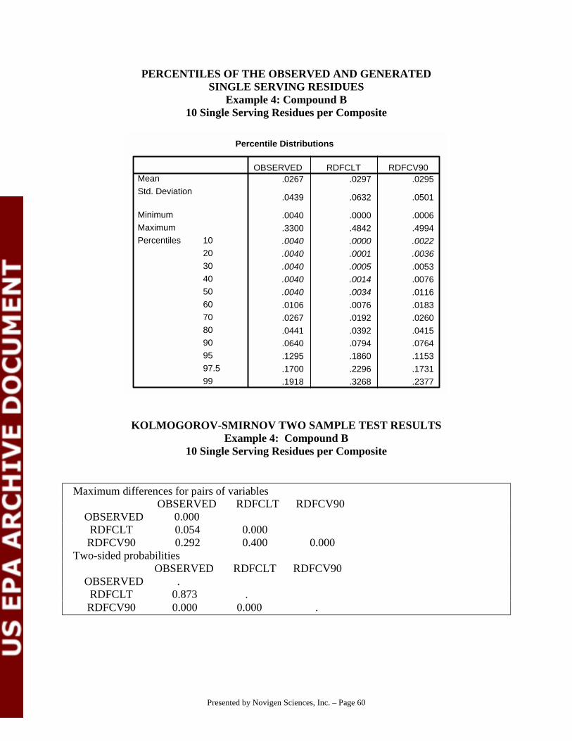
Presented by Novigen Sciences, Inc. – Page 60
PERCENTILES OF THE OBSERVED AND GENERATEDSINGLE SERVING RESIDUES
Example 4: Compound B10 Single Serving Residues per Composite
Percentile Distributions
.0267 .0297 .0295
.0439 .0632 .0501
.0040 .0000 .0006
.3300 .4842 .4994
.0040 .0000 .0022
.0040 .0001 .0036
.0040 .0005 .0053
.0040 .0014 .0076
.0040 .0034 .0116
.0106 .0076 .0183
.0267 .0192 .0260
.0441 .0392 .0415
.0640 .0794 .0764
.1295 .1860 .1153
.1700 .2296 .1731
.1918 .3268 .2377
Mean
Std. Deviation
Minimum
Maximum
10
20
30
40
50
60
70
80
90
95
97.5
99
Percentiles
OBSERVED RDFCLT RDFCV90
KOLMOGOROV-SMIRNOV TWO SAMPLE TEST RESULTSExample 4: Compound B
10 Single Serving Residues per Composite
Maximum differences for pairs of variables OBSERVED RDFCLT RDFCV90 OBSERVED 0.000 RDFCLT 0.054 0.000 RDFCV90 0.292 0.400 0.000 Two-sided probabilities OBSERVED RDFCLT RDFCV90 OBSERVED . RDFCLT 0.873 . RDFCV90 0.000 0.000 .

Presented by Novigen Sciences, Inc. – Page 61
6.2.2.2.2 Using hypothetical data
Four scenarios and sets of data were used. In each case, 10 composite samples of 20 singleserving residues were generated from 10 different lognormal distributions, and single servingresidues were generated for each of the 10 composites using the RDFgen™ approach. Thegenerated and observed single serving residue distributions were compared. The scenariosdiffered with respect to how different the means of the original lognormal distributions(representing potential differences between field) were and how variable the distributions were(representing variability within fields). Three sets of single serving residue distributions weregenerated, the first used the RDFgen™ approach and assumed no additional information aboutthe distributions, the second used the RDFgen™ approach and assumed a constant coefficient ofvariation, while the third used Allender’s single distribution approach.
The distributions generated using the RDFgen™ multi-distribution approach were closer to theoriginal single serving distributions, than those generated using the single lognormal distributionassumption. In addition, upper percentiles of the single distributions generated using theRDFgen™ approach and a “known” coefficient were closer to the observed single servingresidues than those generated using the RDFgen™ approach in the absence of additionalinformation or those generated using the single distribution assumption. The largest impact ofusing the additional information about the relative variability of the distributions (i.e., using aknown coefficient of variation) was observed for the scenarios with small within field variability,i.e., Examples 1 and 2.
Example 1: “Large variability between fields, small variability within field”
Means: random values between 0.001 and 6.000 SD/Mean: random values between 0.5 and 1.5
Original Data RDFgen™ approachPercentile 20 ss in 10
compositesKnown CV = 1 CLT
Allender’sSingle
Distribution10% 0.358 0.253 0.009 0.07720% 0.480 0.421 0.035 0.16030% 0.735 0.616 0.094 0.27040% 1.011 0.894 0.212 0.42250% 1.473 1.246 0.444 0.64160% 1.974 1.774 0.809 0.97370% 2.781 2.423 1.489 1.52280% 3.851 3.630 2.864 2.56990% 6.288 6.049 6.800 5.30995% 8.382 9.034 12.01 9.669
97.5% 11.25 12.07 19.81 16.2699% 14.06 16.70 29.64 29.76
99.5% 16.35 19.81 32.39 44.92
Example 2: “Small variability between fields, small variability within field”
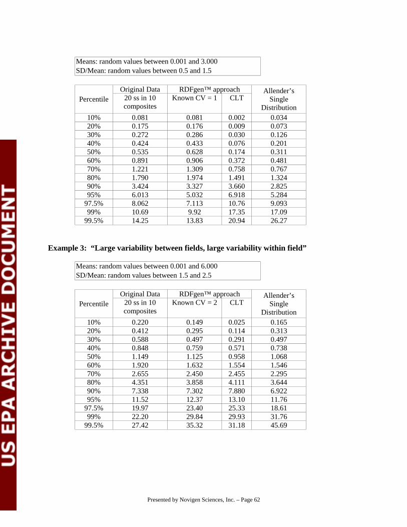
Presented by Novigen Sciences, Inc. – Page 62
Means: random values between 0.001 and 3.000SD/Mean: random values between 0.5 and 1.5
Original Data RDFgen™ approachPercentile 20 ss in 10
compositesKnown CV = 1 CLT
Allender’sSingle
Distribution10% 0.081 0.081 0.002 0.03420% 0.175 0.176 0.009 0.07330% 0.272 0.286 0.030 0.12640% 0.424 0.433 0.076 0.20150% 0.535 0.628 0.174 0.31160% 0.891 0.906 0.372 0.48170% 1.221 1.309 0.758 0.76780% 1.790 1.974 1.491 1.32490% 3.424 3.327 3.660 2.82595% 6.013 5.032 6.918 5.284
97.5% 8.062 7.113 10.76 9.09399% 10.69 9.92 17.35 17.09
99.5% 14.25 13.83 20.94 26.27
Example 3: “Large variability between fields, large variability within field”
Means: random values between 0.001 and 6.000SD/Mean: random values between 1.5 and 2.5
Original Data RDFgen™ approachPercentile 20 ss in 10
compositesKnown CV = 2 CLT
Allender’sSingle
Distribution10% 0.220 0.149 0.025 0.16520% 0.412 0.295 0.114 0.31330% 0.588 0.497 0.291 0.49740% 0.848 0.759 0.571 0.73850% 1.149 1.125 0.958 1.06860% 1.920 1.632 1.554 1.54670% 2.655 2.450 2.455 2.29580% 4.351 3.858 4.111 3.64490% 7.338 7.302 7.880 6.92295% 11.52 12.37 13.10 11.76
97.5% 19.97 23.40 25.33 18.6199% 22.20 29.84 29.93 31.76
99.5% 27.42 35.32 31.18 45.69

Presented by Novigen Sciences, Inc. – Page 63
Example 4: “Large variability between fields, large variability within field”
Means: random values between 0.001 and 3.000SD/Mean: random values between 1.5 and 2.5
Original Data RDFgen™ approachPercentile 20 ss in 10
compositesKnown CV = 2 CLT
Allender’sSingle
Distribution10% 0.080 0.070 0.011 0.04920% 0.156 0.127 0.035 0.09930% 0.251 0.205 0.082 0.16340% 0.352 0.311 0.159 0.24950% 0.501 0.444 0.289 0.37160% 0.672 0.642 0.500 0.55370% 1.053 0.970 0.849 0.84780% 1.648 1.551 1.537 1.39690% 3.158 3.079 3.415 2.78995% 5.675 4.749 6.177 4.940
97.5% 7.697 8.978 11.33 8.10999% 10.42 12.08 13.72 14.43
99.5% 11.77 13.49 14.46 21.37
7. Other
7.1 Water Consumption
The CSFII collected information about non-food based water consumption, that is waterconsumed as “water”, not mixed in foods (e.g., soup) or beverages (e.g., coffee). However, theinformation was collected on only one survey day, and the method used to collect theinformation was different from that used to collect the rest of the of the dietary intakes.Specifically, the information referred to the entire quantity of non-food based water consumedduring that day. That is, no information is available about when, during the day, the water wasconsumed, how often it was consumed during the day, or the various amounts consumed (if itwas consumed more than once).
In the absence of additional data, DEEM™ assumes that the amounts reported apply to all thesurvey days, and allows the incorporation of the water consumption in its exposure assessments.

Presented by Novigen Sciences, Inc. – Page 64
7.2 Missing body weights
The body weights of some of the survey respondents were missing. DEEM™ estimates the bodyweights of these individuals using the reported body weights of individuals in the same age andsex group. Specifically, linear regression models relating body weight and age were derived formales and females in the following age groups:
" infants, ages 0 to 11 months," children ages 1 to 5 years," children ages 6 to 11 years," children ages 12 to 16 years.
These models (see Appendix 2) were used in the estimation of the missing body weights ofinfants and children.
For all other age groups, missing body weights were replaced by the average body weight of theindividuals in the same age and sex group (see Appendix 2).
7.3 Foods with no consumption
EPA has developed a master list of RACs (Appendix 1). The master EPA list contains 458RACs. Each of the foods reported consumed in the CSFII was translated into one or more RACsusing Novigen translation factors. There was no consumption for some of these RACs in one ormore of the surveys (some were reported consumed in the 1989-91 CSFII; some in the 1994-94CSFII, some in neither survey). If the RAC was not consumed in a particular survey, DEEM™assumes that the consumption of that RAC is insignificant for that survey period and assigns avalue of zero. The user is notified that there was no consumption of the particular RAC as a partof the results’ reports.

Presented by Novigen Sciences, Inc. – Page 65
8.0 References
Chin, H.B. (1991). The effect of processing on residues in foods: The food processingindustry’s residue database. In Pesticide Residues and Food Safety: A Harvest ofViewpoints. B.G. Tweedy, H.J. Dishburger, L.G. Ballantine, and J. McCarthy, eds.Washington, DC: American Chemical Society, Washington, DC, 175.
Life Sciences Research Office (LSRO) (1989). Nutrition Monitoring in the United States: AnUpdate Report on Nutrition Monitoring. Prepared for the U.S. Department of Agricultureand the U.S. Department of Health and Human Services. DHHS Publication No. (PHS)89-1255. U.S. Government Printing Office, Washington, D.C.
Mosteller, F. and J.W. Tukey (1977). Data Analysis and Regression. Reading, MA: Addison-Wesley Publishing. Co.
National Research Council (NRC), Committee on Pesticides in the Diets of Infants and Children,Board on Agriculture and Board on Environmental Studies and Toxicology, Commissionon Life Sciences (1993). Pesticides in the Diets of Infants and Children. Washington,DC: National Academy Press.
United States Department of Agriculture (USDA) (1975). Food Yields Summarized by DifferentStages of Preparation. Handbook 102. Washington, D.C.
United States Department of Agriculture (USDA) (1982). Commodity Maps. December.Washington, D.C.
United States Department of Agriculture (USDA) (1992). Nationwide Food ConsumptionSurvey: Continuing Survey of Food Intakes by Individuals 1989-90. Human NutritionInformation Service. Dataset.
United States Department of Agriculture (USDA) (1993). Nationwide Food ConsumptionSurvey: Continuing Survey of Food Intakes by Individuals 1990-91. Human NutritionInformation Service. Dataset.
United States Department of Agriculture (USDA) (1994). Nationwide Food ConsumptionSurvey: Continuing Survey of Food Intakes by Individuals 1991-92. Human NutritionInformation Service. Dataset.
United States Department of Agriculture (USDA) (1995). Food Survey Research Group,Agricultural Research Service (ARS). Nationwide Food Consumption Survey:Continuing Survey of Food Intakes by Individuals 1993-94. Dataset.
United States Department of Agriculture (USDA) (1996). Food Survey Research Group,Agricultural Research Service (ARS). Nationwide Food Consumption Survey:Continuing Survey of Food Intakes by Individuals 1994-95. Dataset.

Presented by Novigen Sciences, Inc. – Page 66
United States Department of Agriculture (USDA) (1996a). Pesticide Data Program, AnnualSummary Calendar Year 1994. Agricultural Marketing Service. Science andTechnology Division. Page 6.
United States Department of Agriculture (USDA) (1996b). Pesticide Data Program AgriculturalMarketing Service. Science and Technology Division. Dataset for calendar year 1994.
United States Department of Agriculture (USDA) (1997a). Food Survey Research Group,Agricultural Research Service (ARS). Nationwide Food Consumption Survey:Continuing Survey of Food Intakes by Individuals 1995-96. Dataset.
United States Department of Agriculture (USDA) (1997b). Food Survey Research Group,Agricultural Research Service (ARS). Design and Operation: Continuing Survey ofFood Intakes by Individuals 1994-96.
United States Department of Agriculture (USDA) (1997a). Pesticide Data Program AgriculturalMarketing Service. Science and Technology Division. Dataset for calendar year 1995.
United States Department of Agriculture (USDA) (1997b). Pesticide Data Program, AnnualSummary Calendar Year 1995. Agricultural Marketing Service. Science andTechnology Division. Page 6.
United States Department of Agriculture (USDA) (1998a). Pesticide Data Program, AnnualSummary Calendar Year 1996. Agricultural Marketing Service. Science andTechnology Division. Page 7 and Page x.
United States Department of Agriculture (USDA) (1998b). Pesticide Data Program AgriculturalMarketing Service. Science and Technology Division. Dataset for calendar year 1996.

Presented by Novigen Sciences, Inc. – Page 67
Figures

Presented by Novigen Sciences, Inc. – Page 68
FIGURE 1COMPONENTS OF A CUMULATIVE RISK ASSESSMENT
USDA CSFIIDemographic, Social,
Geographical Characteristics& Food Consumption Patterns
USDA PDPMultiple CompoundsResidue Distributions
Other FoodResidue Data
PesticideUse
Patterns
Processing Factors
Toxicological Profiles
DietaryExposureEstimates
Residential PesticideUse Patterns
Residue Files
Cumulative Risk
Estimates
AggregateExposure Estimates
Non-dietaryExposure Estimates
CALENDEX™DEEM™
OtherResidue
Adjustments
ResidueFiles
Residue Data

Presented by Novigen Sciences, Inc. – Page 69
FIGURE 2DEFAULT OUTPUT OF THE DEEM™ CHRONIC ANALYSIS MODULE
Exposures Compared to the RfD and NOEL
Novigen Ver. 7.02DEEM Chronic analysis for TEST CHEMICAL (1994-96 data)Residue file name: C:\My Documents\sample outputs\chrntest.RS7 Adjustment factor #2 used.Analysis Date 01-16-2000/08:21:10 Residue file dated: 01-16-2000/08:17:17/1Reference dose (RfD, Chronic) = .01 mg/kg bw/dayNOEL (Chronic) = 1 mg/kg bw/dayCOMMENT 1: sample run=============================================================================== Total exposure by population subgroup-------------------------------------------------------------------------------
Total Exposure ----------------------------------- Population mg/kg Margin of Percent Subgroup body wt/day Exposure of RfD-------------------------------------- ------------- ---------- ---------U.S. Population (total) 0.000305 3,274 3.1%
U.S. Population (spring season) 0.000298 3,353 3.0%U.S. Population (summer season) 0.000294 3,401 2.9%U.S. Population (autumn season) 0.000304 3,292 3.0%U.S. Population (winter season) 0.000327 3,057 3.3%
Northeast region 0.000338 2,960 3.4%Midwest region 0.000301 3,327 3.0%Southern region 0.000263 3,802 2.6%Western region 0.000349 2,866 3.5%
Hispanics 0.000335 2,988 3.3%Non-hispanic whites 0.000315 3,174 3.2%Non-hispanic blacks 0.000233 4,295 2.3%Non-hisp/non-white/non-black 0.000284 3,518 2.8%
All infants (< 1 year) 0.001017 983 10.2%Nursing infants 0.000751 1,332 7.5%Non-nursing infants 0.001095 913 10.9%Children 1-6 yrs 0.001033 968 10.3%Children 7-12 yrs 0.000327 3,054 3.3%
Females 13-19 (not preg or nursing) 0.000131 7,643 1.3%Females 20+ (not preg or nursing) 0.000233 4,301 2.3%Females 13-50 yrs 0.000192 5,198 1.9%Females 13+ (preg/not nursing) 0.000213 4,696 2.1%Females 13+ (nursing) 0.000271 3,688 2.7%
Males 13-19 yrs 0.000129 7,764 1.3%Males 20+ yrs 0.000196 5,104 2.0%Seniors 55+ 0.000278 3,597 2.8%
-------------------------------------------------------------------------------

Presented by Novigen Sciences, Inc. – Page 70
FIGURE 3DEFAULT OUTPUT OF THE DEEM™ CHRONIC ANALYSIS MODULE
Exposures Compared to the Q1*
Novigen Ver. 7.02DEEM Chronic analysis for TEST CHEMICAL (1994-96 data)Residue file name: C:\My Documents\sample outputs\chrntest.RS7 Adjustment factor #2 used.Analysis Date 01-16-2000/08:19:21 Residue file dated: 01-16-2000/08:17:17/1Q* = 0.1COMMENT 1: sample run=============================================================================== Total exposure by population subgroup-------------------------------------------------------------------------------
Total Exposure ----------------------------------- Population mg/kg Lifetime risk Subgroup body wt/day (Q*= .1)-------------------------------------- ------------- -------------U.S. Population (total) 0.000305 3.05E-05
U.S. Population (spring season) 0.000298 2.98E-05U.S. Population (summer season) 0.000294 2.94E-05U.S. Population (autumn season) 0.000304 3.04E-05U.S. Population (winter season) 0.000327 3.27E-05
Northeast region 0.000338 3.38E-05Midwest region 0.000301 3.01E-05Southern region 0.000263 2.63E-05Western region 0.000349 3.49E-05
Hispanics 0.000335 3.35E-05Non-hispanic whites 0.000315 3.15E-05Non-hispanic blacks 0.000233 2.33E-05Non-hisp/non-white/non-black 0.000284 2.84E-05
All infants (< 1 year) 0.001017Nursing infants 0.000751Non-nursing infants 0.001095Children 1-6 yrs 0.001033Children 7-12 yrs 0.000327
Females 13-19 (not preg or nursing) 0.000131Females 20+ (not preg or nursing) 0.000233Females 13-50 yrs 0.000192Females 13+ (preg/not nursing) 0.000213Females 13+ (nursing) 0.000271
Males 13-19 yrs 0.000129Males 20+ yrs 0.000196Seniors 55+ 0.000278
-------------------------------------------------------------------------------

Presented by Novigen Sciences, Inc. – Page 71
FIGURE 4DEEM™ CHRONIC MODULE - COMPLETE COMMODITY CONTRIBUTION ANALYSIS
(ALL INFANTS SUBPOPULATION)
Novigen Ver. 7.02DEEM Chronic analysis for TEST CHEMICAL (1994-96 data)Residue file name: C:\My Documents\sample outputs\chrntest.RS7 Adjustment factor #2 used.Analysis Date 01-16-2000/08:21:16 Residue file dated: 01-16-2000/08:17:17/1Reference dose (RfD, Chronic) = .01 mg/kg bw/dayNOEL (Chronic) = 1 mg/kg bw/dayCOMMENT 1: sample run=============================================================================== Complete commodity contribution analysis for All infants (< 1 year)-------------------------------------------------------------------------------Crop Group = (O) Other Exposure Analysis ---------------------------- Residue Adjustment mg/kg |Margin of| Perc. Food name (ppm) Factors body wt/day|Exposr 1/|of RfD------------------------- ---------- ------------- -----------|---------|------Grapes 0.500000 1.000 0.400 0.0000000 >1000000 0.0%Grapes-raisins 0.500000 4.300 0.400 0.0000044 229,302 0.0%Grapes-juice 0.500000 1.200 0.400 0.0000944 10,596 0.9%Bananas 0.500000 1.000 1.000 0.0005991 1,669 6.0%Bananas-dried 0.500000 3.900 1.000 0.0001370 7,299 1.4%Grapes-leaves 0.500000 1.000 0.400 no exposureGrapes-wine and sherry 0.500000 1.000 0.400 0.0000000 >1000000 0.0%Bananas-juice 0.500000 1.000 1.000 0.0000232 43,036 0.2%Grapes-juice-concentrate 0.500000 3.600 0.400 0.0001216 8,225 1.2% ----------- -------- ------- Crop group subtotal 0.0009797 1,021 9.8%
Crop Group = (10) Citrus Fruits Exposure Analysis ---------------------------- Residue Adjustment mg/kg |Margin of| Perc. Food name (ppm) Factors body wt/day|Exposr 1/|of RfD------------------------- ---------- ------------- -----------|---------|------Grapefruit-peeled fruit 0.040000 1.000 0.200 no exposureGrapefruit-juice 0.040000 2.100 0.200 0.0000006 >1000000 0.0%Grapefruit-juice-concentr 0.040000 8.260 0.200 no exposureGrapefruit peel 0.040000 1.000 0.200 no exposure ----------- -------- ------- Crop group subtotal 0.0000006 >1000000 0.0%Crop Group = (11) Pome Fruits Exposure Analysis ---------------------------- Residue Adjustment mg/kg |Margin of| Perc. Food name (ppm) Factors body wt/day|Exposr 1/|of RfD------------------------- ---------- ------------- -----------|---------|------Apples 0.010000 1.000 0.500 0.0000099 100,805 0.1%Apples-dried 0.010000 8.000 0.500 0.0000006 >1000000 0.0%Apples-juice/cider 0.010000 1.300 0.500 0.0000098 102,088 0.1%Apples-juice-concentrate 0.010000 3.900 0.500 0.0000162 61,905 0.2% ----------- -------- ------- Crop group subtotal 0.0000365 27,383 0.4%
Population subgroup total 0.0010169 983 10.2%-------------------------------------------------------------------------------1. Margin of Exposure = NOEL / Dietary Exposure

Presented by Novigen Sciences, Inc. – Page 72
FIGURE 5DEEM™ CHRONIC MODULE - CRITICAL COMMODITY CONTRIBUTION ANALYSIS
(ALL INFANTS SUBPOPULATION)
Novigen Ver. 7.02DEEM Chronic analysis for TEST CHEMICAL (1994-96 data)Residue file name: C:\My Documents\sample outputs\chrntest.RS7 Adjustment factor #2 used.Analysis Date 01-16-2000/08:21:16 Residue file dated: 01-16-2000/08:17:17/1NOEL (Chronic) = 1 mg/kg bw/dayCOMMENT 1: sample run=============================================================================== Critical Commodity Contribution Analysis for All infants (< 1 year)
Total Exposure =.0010169 mg/kg bw/day
Crop groups with total exposure contribution > 5% Foods/Foodforms with exposure contribution > 1%-------------------------------------------------------------------------------
Crop group ------------ Exposure Analysis ----------- Food mg/kg |% of Total| Percent | Margin Foodform body wt/day| Exposure | of NOEL |of Exposr---------------------------------- -----------|----------|-------- |---------
Crop Group = (O) Other Grapes-juice 0.0000944 9.28% 0.0% 10,596 Bananas 0.0005991 58.92% 0.1% 1,669 Bananas-dried 0.0001370 13.47% 0.0% 7,299 Bananas-juice 0.0000232 2.29% 0.0% 43,036 Grapes-juice-concentrate 0.0001216 11.96% 0.0% 8,225---------------------------------- -----------|----------|-------- |--------- Total for crop group 0.0009797 96.35% 0.1% 1,021
Crop Group = (11) Pome Fruits Apples-juice-concentrate 0.0000162 1.59% 0.0% 61,905---------------------------------- -----------|----------|-------- |--------- Total for crop group 0.0000365 3.59% 0.0% 27,383
Total for crop groups listed above: 0.0010163 99.94% 0.1% 984-------------------------------------------------------------------------------
1. Margin of Exposure = NOEL / Dietary Exposure

Presented by Novigen Sciences, Inc. – Page 73
FIGURE 6DEEM™ CHRONIC MODULE - RESIDUE FILE SUMMARY
Novigen Ver. 7.02DEEM Chronic analysis for TEST CHEMICAL 1994-96 dataResidue file: C:\My Documents\sample outputs\chrntest.RS7 Adjust. #2 usedAnalysis Date 01-16-2000 Residue file dated: 01-16-2000/08:17:17/1Reference dose (RfD) = 0.01 (NOEL) = 1 mg/kg bw/dayComment:sample run--------------------------------------------------------------------------------Food Crop RESIDUE Adj.Factors CommentCode Grp Food Name (ppm) #1 #2---- ---- ------------------------------- ---------- ------ ------ ------- 13 O Grapes 0.500000 1.000 0.400 14 O Grapes-raisins 0.500000 4.300 0.400 15 O Grapes-juice 0.500000 1.200 0.400 22 10 Grapefruit-peeled fruit 0.040000 1.000 0.200 23 10 Grapefruit-juice 0.040000 2.100 0.200 52 11 Apples 0.010000 1.000 0.500 53 11 Apples-dried 0.010000 8.000 0.500 54 11 Apples-juice/cider 0.010000 1.300 0.500 72 O Bananas 0.500000 1.000 1.000 73 O Bananas-dried 0.500000 3.900 1.000 195 O Grapes-leaves 0.500000 1.000 0.400 315 O Grapes-wine and sherry 0.500000 1.000 0.400 377 11 Apples-juice-concentrate 0.010000 3.900 0.500 378 O Bananas-juice 0.500000 1.000 1.000 392 O Grapes-juice-concentrate 0.500000 3.600 0.400 441 10 Grapefruit-juice-concentrate 0.040000 8.260 0.200 448 10 Grapefruit peel 0.040000 1.000 0.200

Presented by Novigen Sciences, Inc. – Page 74
FIGURE 7DEFAULT OUTPUT OF THE DEEM™ ACUTE MODULE
Novigen Sciences, Incorporated Ver. 7.02DEEM ACUTE analysis for NOVICHEM (1994-96 data)Residue file: acmctest.RS7 Adjustment factor #2 NOT used.Analysis Date: 01-16-2000/21:01:54 Residue file dated: 10-06-1999/11:17:05/1NOEL (Acute) = 0.250000 mg/kg body-wt/dayDaily totals for food and foodform consumption used.MC iterations = 100 MC list in residue file MC seed = 1Run Comment: TEST SERIES FOR DEEM ACUTE MODULES===============================================================================
All infants Daily Exposure Analysis 1/----------- (mg/kg body-weight/day) per Capita per User ----------- ----------- Mean 0.000066 0.000086 Standard Deviation 0.000168 0.000187 Margin of Exposure 2/ 3,783 2,890
Percent of Person-Days that are User-Days = 76.39%
Estimated percentile of user-days falling below calculated exposure in mg/kg body-wt/day with Margin of Exposure (MOE)
Percentile Exposure MOE Percentile Exposure MOE ---------- ---------- --------- ---------- ---------- --------- 10.00 0.000000 797,317 90.00 0.000192 1,298 20.00 0.000003 74,684 95.00 0.000390 641 30.00 0.000013 19,789 97.50 0.000573 436 40.00 0.000033 7,559 99.00 0.000872 286 50.00 0.000049 5,142 99.50 0.001003 249 60.00 0.000061 4,119 99.75 0.001027 243 70.00 0.000073 3,440 99.90 0.001068 234 80.00 0.000092 2,703
Estimated percentile of per-capita days falling below calculated exposure in mg/kg body-wt/day with Margin of Exposure (MOE)
Percentile Exposure MOE Percentile Exposure MOE ---------- ---------- --------- ---------- ---------- --------- 10.00 0.000000 >1,000,000 90.00 0.000139 1,792 20.00 0.000000 >1,000,000 95.00 0.000324 772 30.00 0.000000 >1,000,000 97.50 0.000453 551 40.00 0.000005 49,400 99.00 0.000686 364 50.00 0.000023 11,014 99.50 0.000888 281 60.00 0.000043 5,831 99.75 0.001010 247 70.00 0.000061 4,075 99.90 0.001056 236 80.00 0.000078 3,186-------------------------------------------------------------------------------1/ Analysis based on all two-day participant records in CSFII 1994-96 survey.2/ Margin of Exposure = NOEL/ Dietary Exposure.

Presented by Novigen Sciences, Inc. – Page 75
FIGURE 8DEEM™ ACUTE MODULE PLOT FILE
Novigen Sciences, Incorporated Ver. 7.02DEEM ACUTE PLOT FILE for NOVICHEM (1994-96 data)Residue file: acmctest.RS7 Adjustment factor #2 NOT used.Analysis Date: 01-16-2000/21:01:54 Residue file dated: 10-06-1999/11:17:05/1NOEL (Acute) = 0.250000 mg/kg body-wt/dayDaily totals for food and foodform consumption used.MC iterations = 100 MC list in residue file MC seed = 1Run Comment: TEST SERIES FOR DEEM ACUTE MODULES===============================================================================Number of populations included in this file: 1Populations:
1 = All infants
Pops: , 1,Means:, 0.000086,PCTLS 90.00, 0.000000, 80.00, 0.000003, . . 2.50, 0.000573, 1.00, 0.000872, 0.50, 0.001003, 0.25, 0.001027, 0.10, 0.001068, 0.00, 0.010247,
All infantsTotal person days (weighted & unweighted) =, 7544592, 718Total user days (weighted & unweighted) =, 5763691, 521Bin totals based on 100 iterations.BIN TOTALS: Users , ---------Exposure Bin-------- , Low Bound, High bound 47151610, 0.0 , 0.00000000 44419194, 0.00000000, 0.00000133 19277563, 0.00000133, 0.00000266 8509380, 0.00000266, 0.00000398 5353774, 0.00000398, 0.00000531 . . 9494, 0.00511968, 0.00517087 43516, 0.00554388, 0.00559932 6376, 0.00565531, 0.00571186 6490, 0.00650063, 0.00656564 11713, 0.00669761, 0.00676458 24969, 0.00747231, 0.00754703 5727, 0.00841998, 0.00850418 13959, 0.00987309, 0.00997183 9591, 0.01017226, 0.01024721

Presented by Novigen Sciences, Inc. – Page 76
FIGURE 9DEEM™ ACUTE MODULE CRITICAL EXPOSRE CONTRIBUTION ANALYSIS
Novigen Sciences, IncorporatedDEEM Acute Critical Exposure Contribution Analysis (Ver 7.02)CSFII 1994-96Residue file = C:\My Documents\sample outputs\acmctest.RS7Acute report = C:\My Documents\sample outputs\acmctest.AC7Date and time of analysis: 01-16-2000 21:00:48Minimum exposure contribution = 1%Monte Carlo Iterations = 100 Seed = 1Exposures divided by body weightSubpopulations: 1 All infants
All infantsLow percentile for CEC records: 95 Exposure (mg/day) = 0.000390High percentile for CEC records: 100 Exposure (mg/day) = 0.010247Number of actual records in this interval: 3191
Critical foods/foodforms for this population (as derived from these records): N=number of appearances in all records (including duplicates) %=percent of total exposure for all records (including duplicates)Food FF N % Name398, 16, 2780, 67.11, Milk-based water-Pasteurized 65, 31, 99, 7.89, Peaches-Canned: NFS398, 31, 303, 5.42, Milk-based water-Canned: NFS320, 16, 2775, 2.86, Milk sugar (lactose)-Pasteurized318, 16, 2775, 2.27, Milk-nonfat solids-Pasteurized319, 16, 2768, 1.69, Milk-fat solids-Pasteurized 54, 11, 79, 1.49, Apples-juice/cider-Uncooked320, 31, 436, 1.46, Milk sugar (lactose)-Canned: NFS159, 34, 622, 1.15, Tomatoes-whole-Canned: Boiled 65, 11, 11, 1.14, Peaches-Uncooked . .53, 14, 10, 0.00, Apples-dried-Boiled 65, 14, 6, 0.00, Peaches-Boiled 53, 18, 1, 0.00, Apples-dried-Dried320, 12, 3, 0.00, Milk sugar (lactose)-Cooked: NFS318, 12, 3, 0.00, Milk-nonfat solids-Cooked: NFS 52, 31, 5, 0.00, Apples-Canned: NFS159, 33, 1, 0.00, Tomatoes-whole-Canned: Baked 17, 14, 84, 0.00, Strawberries-Boiled 52, 14, 4, 0.00, Apples-Boiled398, 12, 100, 0.00, Milk-based water-Cooked: NFS392, 31, 2, 0.00, Grapes-juice-concentrate-Canned: NFS398, 32, 97, 0.00, Milk-based water-Canned: Cooked398, 45, 100, 0.00, Milk-based water-Frozen: Fried 14, 14, 7, 0.00, Grapes-raisins-Boiled

Presented by Novigen Sciences, Inc. – Page 77
FIGURE 9 (CONT’D)
Number of printed records = 500Number of records represented = 1791 (nf = number of foods/ff reported for this daily exposure amount (exceeding minimum contribution) (nx = number of times this exposure amount was computed for the same person on the same day.)
Demographic data for each record:Demographic data for each record:Exposure contribution data by food/ff consumed (nf lines):Pid day sex age bw-kg nf nx Tot expos samplwt Line food ff amt(g) residue adj#1 adj#2 Cntrbtn Percent
63 2 M 7M 8.18 1 1 0.010247 9591 1 65 31 139.4 0.6 1 1 0.010223 99.76
71 1 F 9M 9.55 1 1 0.009938 13959 1 65 11 157 0.6 1 1 0.009869 99.3
12 1 M 5M 6.82 1 1 0.008473 5727 1 65 31 96.2 0.6 1 1 0.008466 99.91
54 1 M 7M 7.73 1 3 0.007485 8323 1 65 31 96.4 0.6 1 1 0.007485 100
27 2 M 8M 7.27 1 1 0.006755 11713 1 65 31 81.6 0.6 1 1 0.006732 99.65
68 1 M 8M 10 1 1 0.006539 6490 1 65 31 108.8 0.6 1 1 0.006528 99.83
32 2 F 10M 8.64 1 1 0.00569 6376 1 65 31 81.6 0.6 1 1 0.005669 99.63
55 1 M 9M 10.45 1 1 0.005567 21758 1 65 31 96.4 0.6 1 1 0.005533 99.39
55 1 M 9M 10.45 1 1 0.00557 21758 1 65 31 96.4 0.6 1 1 0.00553 99.4
67 2 F 11M 9.55 2 1 0.00515 9494 1 65 11 78.5 0.6 1 1 0.00493 95.73
67 2 F 11M 9.55 2 1 0.00515 9494 2 398 16 348.9 0.005 1 1 0.00018 3.55
15 1 M 6M 7.27 1 1 0.00499 8834 1 65 31 60.4 0.6 1 1 0.00498 99.94
29 2 M 6M 6.82 1 1 0.00483 4161 1 65 31 54.4 0.6 1 1 0.00479 99.19
34 1 M 7M 6.82 1 1 0.00423 2978 1 65 31 48 0.6 1 1 0.00422 99.97
22 2 M 8M 8.18 1 1 0.00416 4532 1 54 11 542.3 0.06274 1 1 0.00416 99.92
etc.
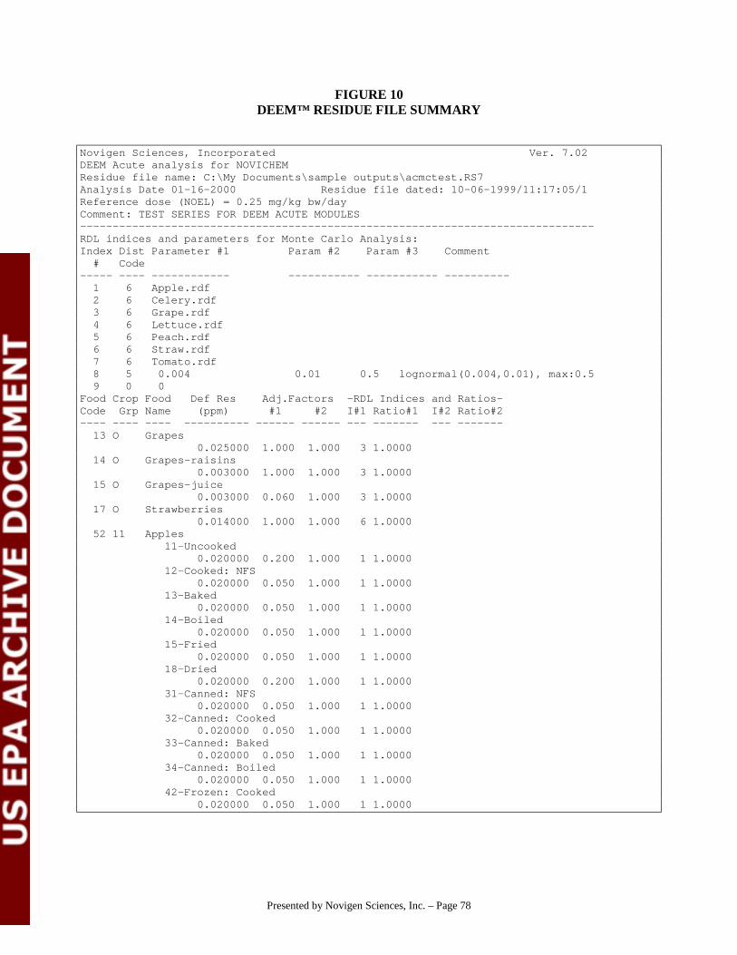
Presented by Novigen Sciences, Inc. – Page 78
FIGURE 10DEEM™ RESIDUE FILE SUMMARY
Novigen Sciences, Incorporated Ver. 7.02DEEM Acute analysis for NOVICHEMResidue file name: C:\My Documents\sample outputs\acmctest.RS7Analysis Date 01-16-2000 Residue file dated: 10-06-1999/11:17:05/1Reference dose (NOEL) = 0.25 mg/kg bw/dayComment: TEST SERIES FOR DEEM ACUTE MODULES-------------------------------------------------------------------------------RDL indices and parameters for Monte Carlo Analysis:Index Dist Parameter #1 Param #2 Param #3 Comment # Code----- ---- ------------ ----------- ----------- ---------- 1 6 Apple.rdf 2 6 Celery.rdf 3 6 Grape.rdf 4 6 Lettuce.rdf 5 6 Peach.rdf 6 6 Straw.rdf 7 6 Tomato.rdf 8 5 0.004 0.01 0.5 lognormal(0.004,0.01), max:0.5 9 0 0Food Crop Food Def Res Adj.Factors -RDL Indices and Ratios-Code Grp Name (ppm) #1 #2 I#1 Ratio#1 I#2 Ratio#2---- ---- ---- ---------- ------ ------ --- ------- --- ------- 13 O Grapes 0.025000 1.000 1.000 3 1.0000 14 O Grapes-raisins 0.003000 1.000 1.000 3 1.0000 15 O Grapes-juice 0.003000 0.060 1.000 3 1.0000 17 O Strawberries 0.014000 1.000 1.000 6 1.0000 52 11 Apples 11-Uncooked 0.020000 0.200 1.000 1 1.0000 12-Cooked: NFS 0.020000 0.050 1.000 1 1.0000 13-Baked 0.020000 0.050 1.000 1 1.0000 14-Boiled 0.020000 0.050 1.000 1 1.0000 15-Fried 0.020000 0.050 1.000 1 1.0000 18-Dried 0.020000 0.200 1.000 1 1.0000 31-Canned: NFS 0.020000 0.050 1.000 1 1.0000 32-Canned: Cooked 0.020000 0.050 1.000 1 1.0000 33-Canned: Baked 0.020000 0.050 1.000 1 1.0000 34-Canned: Boiled 0.020000 0.050 1.000 1 1.0000 42-Frozen: Cooked 0.020000 0.050 1.000 1 1.0000
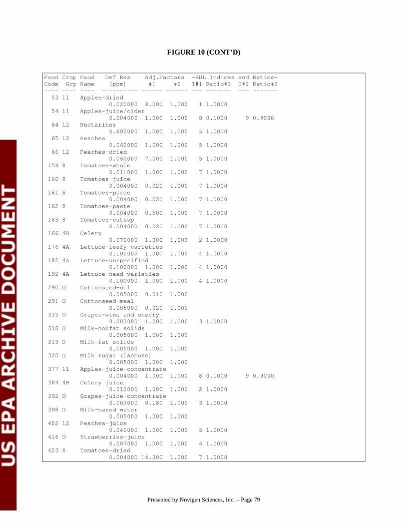
Presented by Novigen Sciences, Inc. – Page 79
FIGURE 10 (CONT’D)
Food Crop Food Def Res Adj.Factors -RDL Indices and Ratios-Code Grp Name (ppm) #1 #2 I#1 Ratio#1 I#2 Ratio#2---- ---- ---- ---------- ------ ------ --- ------- --- ------- 53 11 Apples-dried 0.020000 8.000 1.000 1 1.0000 54 11 Apples-juice/cider 0.004000 1.000 1.000 8 0.1000 9 0.9000 64 12 Nectarines 0.600000 1.000 1.000 5 1.0000 65 12 Peaches 0.060000 1.000 1.000 5 1.0000 66 12 Peaches-dried 0.060000 7.000 1.000 5 1.0000 159 8 Tomatoes-whole 0.011000 1.000 1.000 7 1.0000 160 8 Tomatoes-juice 0.004000 0.020 1.000 7 1.0000 161 8 Tomatoes-puree 0.004000 0.020 1.000 7 1.0000 162 8 Tomatoes-paste 0.004000 0.500 1.000 7 1.0000 163 8 Tomatoes-catsup 0.004000 0.020 1.000 7 1.0000 166 4B Celery 0.070000 1.000 1.000 2 1.0000 176 4A Lettuce-leafy varieties 0.100000 1.000 1.000 4 1.0000 182 4A Lettuce-unspecified 0.100000 1.000 1.000 4 1.0000 192 4A Lettuce-head varieties 0.100000 1.000 1.000 4 1.0000 290 O Cottonseed-oil 0.005000 0.010 1.000 291 O Cottonseed-meal 0.005000 0.020 1.000 315 O Grapes-wine and sherry 0.003000 1.000 1.000 3 1.0000 318 D Milk-nonfat solids 0.005000 1.000 1.000 319 D Milk-fat solids 0.005000 1.000 1.000 320 D Milk sugar (lactose) 0.005000 1.000 1.000 377 11 Apples-juice-concentrate 0.004000 1.000 1.000 8 0.1000 9 0.9000 384 4B Celery juice 0.012000 1.000 1.000 2 1.0000 392 O Grapes-juice-concentrate 0.003000 0.180 1.000 3 1.0000 398 D Milk-based water 0.005000 1.000 1.000 402 12 Peaches-juice 0.040000 1.000 1.000 5 1.0000 416 O Strawberries-juice 0.007000 1.000 1.000 6 1.0000 423 8 Tomatoes-dried 0.004000 14.300 1.000 7 1.0000
Presented by Novigen Sciences, Inc. – Page 80
Appendix 1
Listing of Foods, Food Forms, and Crop Groups

APPENDIX 1LISTING OF FOODS, FOOD FORMS, AND CROP GROUPS
Food Crop Food Name Adjust CSFII CSFIICode Grp \Food Form Factor 89-92 94-96----------------------------------------------------------------------------- 1 13A Blackberries 1.00 11 Uncooked X X 13 Baked X X 14 Boiled X X 31 Canned: NFS X X 34 Canned: Boiled X X 41 Frozen: NFS X X 2 13A Boysenberries 1.00 31 Canned: NFS X X 34 Canned: Boiled X X 41 Frozen: NFS X X 3 13A Dewberries 1.00 4 13A Loganberries 1.00 5 13A Raspberries 1.00 11 Uncooked X X 13 Baked X X 14 Boiled X X 31 Canned: NFS X X 34 Canned: Boiled X 41 Frozen: NFS X X 6 13A Youngberries 1.00 7 13B Blueberries 1.00 11 Uncooked X X 12 Cooked: NFS X X 13 Baked X X 14 Boiled X X 15 Fried X X 31 Canned: NFS X X 41 Frozen: NFS X X 8 O Cranberries 1.00 11 Uncooked X X 12 Cooked: NFS X X 13 Baked X X 18 Dried X X 31 Canned: NFS X X 42 Frozen: Cooked X X 9 O Cranberries-juice 1.10 11 Uncooked X X 12 Cooked: NFS X X 31 Canned: NFS X X 10 13B Currants 1.00 11 Uncooked X X 11 13B Elderberries 1.00 12 13B Gooseberries 1.00 13 O Grapes 1.00 11 Uncooked X X 12 Cooked: NFS X X 31 Canned: NFS X X

Presented by Novigen Sciences, Inc. – Page 82
APPENDIX 1 (CONT’D)
Food Crop Food Name Adjust CSFII CSFIICode Grp \Food Form Factor 89-92 94-96----------------------------------------------------------------------------- 41 Frozen: NFS X X 14 O Grapes-raisins 4.30 11 Uncooked X X 12 Cooked: NFS X X 13 Baked X X 14 Boiled X X 18 Dried X X 42 Frozen: Cooked X X 15 O Grapes-juice 1.20 11 Uncooked X X 12 Cooked: NFS X X 14 Boiled X X 31 Canned: NFS X X 34 Canned: Boiled X X 41 Frozen: NFS X 16 13B Huckleberries 1.00 17 O Strawberries 1.00 11 Uncooked X X 12 Cooked: NFS X X 13 Baked X X 14 Boiled X X 31 Canned: NFS X X 34 Canned: Boiled X X 41 Frozen: NFS X X 18 O Juneberry 1.00 19 O Mulberries 1.00 11 Uncooked X X 20 10 Citrus citron 1.00 13 Baked X X 14 Boiled X X 22 10 Grapefruit-peeled fruit 1.00 11 Uncooked X X 12 Cooked: NFS X 31 Canned: NFS X X 23 10 Grapefruit-juice 2.10 11 Uncooked X X 31 Canned: NFS X X 24 10 Kumquats 1.00 26 10 Lemons-peeled fruit 1.00 11 Uncooked X X 12 Cooked: NFS X X 31 Canned: NFS X X 27 10 Lemons-peel 1.00 11 Uncooked X X 13 Baked X X 14 Boiled X X 31 Canned: NFS X 34 Canned: Boiled X X 41 Frozen: NFS X X 28 10 Lemons-juice 2.00 11 Uncooked X X 12 Cooked: NFS X X

Presented by Novigen Sciences, Inc. – Page 83
APPENDIX 1 (CONT’D)
Food Crop Food Name Adjust CSFII CSFIICode Grp \Food Form Factor 89-92 94-96----------------------------------------------------------------------------- 13 Baked X X 14 Boiled X X 15 Fried X X 31 Canned: NFS X X 32 Canned: Cooked X X 34 Canned: Boiled X X 41 Frozen: NFS X X 42 Frozen: Cooked X X 30 10 Limes-peeled fruit 1.00 11 Uncooked X X 31 10 Limes-peel 1.00 13 Baked X X 14 Boiled X X 32 10 Limes-juice 2.00 11 Uncooked X X 31 Canned: NFS X X 32 Canned: Cooked X X 34 Canned: Boiled X X 41 Frozen: NFS X X 33 10 Oranges-juice-concentrate 6.70 11 Uncooked X X 12 Cooked: NFS X X 13 Baked X 14 Boiled X X 31 Canned: NFS X X 41 Frozen: NFS X X 42 Frozen: Cooked X X 34 10 Oranges-peeled fruit 1.00 11 Uncooked X X 12 Cooked: NFS X X 31 Canned: NFS X X 35 10 Oranges-peel 1.00 11 Uncooked X X 12 Cooked: NFS X X 31 Canned: NFS X X 41 Frozen: NFS X X 36 10 Oranges-juice 1.80 11 Uncooked X X 12 Cooked: NFS X X 31 Canned: NFS X X 41 Frozen: NFS X X 37 10 Tangelos 1.00 38 10 Tangerines 1.00 11 Uncooked X X 31 Canned: NFS X X 41 Frozen: NFS X 39 10 Tangerines-juice 2.30 11 Uncooked X 31 Canned: NFS X X 41 Frozen: NFS X 40 14 Almonds 1.00 11 Uncooked X X

Presented by Novigen Sciences, Inc. – Page 84
APPENDIX 1 (CONT’D)
Food Crop Food Name Adjust CSFII CSFIICode Grp \Food Form Factor 89-92 94-96----------------------------------------------------------------------------- 12 Cooked: NFS X X 13 Baked X X 14 Boiled X X 18 Dried X X 41 Frozen: NFS X X 41 14 Brazil nuts 1.00 11 Uncooked X X 13 Baked X X 14 Boiled X X 16 Pasteurized X X 42 14 Cashews 1.00 11 Uncooked X X 13 Baked X X 14 Boiled X X 43 14 Chestnuts 1.00 12 Cooked: NFS X 13 Baked X 44 14 Filberts (hazelnuts) 1.00 11 Uncooked X X 13 Baked X X 14 Boiled X X 45 14 Hickory nuts 1.00 11 Uncooked X 46 14 Macadamia nuts (bush nuts) 1.00 13 Baked X X 47 14 Pecans 1.00 11 Uncooked X X 13 Baked X X 14 Boiled X X 48 14 Walnuts 1.00 11 Uncooked X X 12 Cooked: NFS X X 13 Baked X X 49 14 Butter nuts 1.00 50 O Pistachio nuts 1.00 11 Uncooked X X 12 Cooked: NFS X X 13 Baked X X 51 14 Beechnuts 1.00 52 11 Apples 1.00 11 Uncooked X X 12 Cooked: NFS X X 13 Baked X X 14 Boiled X X 15 Fried X X 18 Dried X X 31 Canned: NFS X X 32 Canned: Cooked X X 33 Canned: Baked X X 34 Canned: Boiled X X 42 Frozen: Cooked X X

Presented by Novigen Sciences, Inc. – Page 85
APPENDIX 1 (CONT’D)
Food Crop Food Name Adjust CSFII CSFIICode Grp \Food Form Factor 89-92 94-96----------------------------------------------------------------------------- 53 11 Apples-dried 8.00 13 Baked X X 14 Boiled X X 18 Dried X X 42 Frozen: Cooked X 54 11 Apples-juice/cider 1.30 11 Uncooked X X 12 Cooked: NFS X 14 Boiled X X 31 Canned: NFS X X 41 Frozen: NFS X 55 11 Crabapples 1.00 31 Canned: NFS X 56 11 Pears 1.00 11 Uncooked X X 12 Cooked: NFS X X 13 Baked X 14 Boiled X X 31 Canned: NFS X X 57 11 Pears-dried 6.25 13 Baked X X 14 Boiled X 18 Dried X X 58 11 Quinces 1.00 59 12 Apricots 1.00 11 Uncooked X X 12 Cooked: NFS X X 14 Boiled X X 31 Canned: NFS X X 34 Canned: Boiled X X 60 12 Apricots-dried 6.00 13 Baked X X 14 Boiled X X 18 Dried X X 61 12 Cherries 1.00 11 Uncooked X X 12 Cooked: NFS X X 13 Baked X X 14 Boiled X X 31 Canned: NFS X X 33 Canned: Baked X X 41 Frozen: NFS X X 62 12 Cherries-dried 4.00 63 12 Cherries-juice 1.50 13 Baked X 14 Boiled X X 31 Canned: NFS X X 41 Frozen: NFS X 64 12 Nectarines 1.00 11 Uncooked X X 65 12 Peaches 1.00 11 Uncooked X X

Presented by Novigen Sciences, Inc. – Page 86
APPENDIX 1 (CONT’D)
Food Crop Food Name Adjust CSFII CSFIICode Grp \Food Form Factor 89-92 94-96----------------------------------------------------------------------------- 12 Cooked: NFS X X 13 Baked X X 14 Boiled X X 31 Canned: NFS X X 41 Frozen: NFS X X 66 12 Peaches-dried 7.00 14 Boiled X 18 Dried X X 67 12 Plums (damsons) 1.00 11 Uncooked X X 12 Cooked: NFS X X 31 Canned: NFS X X 42 Frozen: Cooked X X 51 Cured: NFS (smoked/pickled/saltd) X 68 12 Plums-prunes (dried) 5.00 13 Baked X X 14 Boiled X X 18 Dried X X 31 Canned: NFS X X 69 12 Plums/prune-juice 1.40 11 Uncooked X X 31 Canned: NFS X X 70 O Avocados 1.00 11 Uncooked X X 72 O Bananas 1.00 11 Uncooked X X 12 Cooked: NFS X X 13 Baked X X 14 Boiled X X 15 Fried X X 31 Canned: NFS X X 32 Canned: Cooked X X 73 O Bananas-dried 3.90 13 Baked X X 15 Fried X X 18 Dried X X 32 Canned: Cooked X 74 O Coconut 1.00 11 Uncooked X X 13 Baked X X 14 Boiled X X 75 O Coconut-dried (copra) 2.10 12 Cooked: NFS X 13 Baked X X 14 Boiled X X 18 Dried X X 76 O Coconut-water 1.00 11 Uncooked X 14 Boiled X X 77 O Dates 1.00 13 Baked X X 14 Boiled X X

Presented by Novigen Sciences, Inc. – Page 87
APPENDIX 1 (CONT’D)
Food Crop Food Name Adjust CSFII CSFIICode Grp \Food Form Factor 89-92 94-96----------------------------------------------------------------------------- 18 Dried X X 78 O Figs 1.00 11 Uncooked X X 13 Baked X X 79 O Guava 1.00 11 Uncooked X X 12 Cooked: NFS X X 31 Canned: NFS X X 80 O Mangoes 1.00 11 Uncooked X X 12 Cooked: NFS X X 31 Canned: NFS X X 81 11 Loquats 1.00 82 O Olives 1.00 60 Canned: Cured X X 84 O Papayas-pulp 1.00 11 Uncooked X X 12 Cooked: NFS X X 85 O Papayas-dried 1.80 18 Dried X 86 O Papayas-juice 1.50 11 Uncooked X X 87 O Pawpaws 1.00 88 O Persimmons 1.00 11 Uncooked X X 89 O Pineapples-peeled fruit 1.00 11 Uncooked X X 12 Cooked: NFS X X 13 Baked X X 14 Boiled X X 31 Canned: NFS X X 33 Canned: Baked X X 41 Frozen: NFS X X 90 O Pineapples-dried 5.00 18 Dried X X 91 O Pineapples-juice 1.70 11 Uncooked X X 12 Cooked: NFS X X 31 Canned: NFS X X 42 Frozen: Cooked X X 92 O Passion fruit (granadilla) 1.00 31 Canned: NFS X X 93 O Pomegranates 1.00 11 Uncooked X X 94 O Plantains-ripe 1.00 11 Uncooked X X 14 Boiled X X 15 Fried X X 95 O Lychees (litchi)/fresh 1.00 96 O Lychee-dried 1.85 97 O Kiwi fruit 1.00 11 Uncooked X X

Presented by Novigen Sciences, Inc. – Page 88
APPENDIX 1 (CONT’D)
Food Crop Food Name Adjust CSFII CSFIICode Grp \Food Form Factor 89-92 94-96----------------------------------------------------------------------------- 31 Canned: NFS X 98 O Acerola 1.00 99 O Ginkgo nuts 1.00 100 O Maney (mammee apple) 1.00 11 Uncooked X 101 O Pitanga (surinam cherry) 1.00 102 O Soursop (annona muricata) 1.00 11 Uncooked X 103 O Sugar apples (sweetsop) 1.00 104 O Bread fruit 1.00 14 Boiled X 105 O Bread nuts 1.00 106 O Carambola (starfruit) 1.00 11 Uncooked X 107 O Cherimoya 1.00 108 O Longan fruit 1.00 109 O Genip (spanish lime) 1.00 110 O Chocolate-cocoa butter 1.00 12 Cooked: NFS X X 111 O Chocolate 1.00 12 Cooked: NFS X X 13 Baked X X 14 Boiled X X 31 Canned: NFS X X 32 Canned: Cooked X X 41 Frozen: NFS X X 112 O Coffee 1.00 12 Cooked: NFS X X 14 Boiled X X 113 O Tea 1.00 12 Cooked: NFS X X 114 1AB Chicory 1.00 115 19B Anise 1.00 14 Boiled X X 52 Cured: Cooked(smokd/pickld/saltd) X X 116 19A Basil 1.00 13 Baked X X 14 Boiled X X 117 19B Caraway 1.00 13 Baked X X 118 19B Cassia 1.00 119 19B Cinnamon 1.00 11 Uncooked X X 12 Cooked: NFS X X 13 Baked X X 120 19B Clove 1.00 12 Cooked: NFS X X 121 19B Coriander 1.00 12 Cooked: NFS X X 122 19B Cumin 1.00 11 Uncooked X X 12 Cooked: NFS X X

Presented by Novigen Sciences, Inc. – Page 89
APPENDIX 1 (CONT’D)
Food Crop Food Name Adjust CSFII CSFIICode Grp \Food Form Factor 89-92 94-96----------------------------------------------------------------------------- 14 Boiled X X 42 Frozen: Cooked X 52 Cured:Cooked(smokd/pickld/saltd) X X 123 19A Dill 1.00 13 Baked X 14 Boiled X X 124 1CD Ginger 1.00 11 Uncooked X X 12 Cooked: NFS X X 13 Baked X X 14 Boiled X X 125 O Hops 1.00 99 Alcohol/Fermented/Distilled X X 126 1AB Horseradish 1.00 12 Cooked: NFS X X 14 Boiled X X 34 Canned: Boiled X X 51 Cured: NFS (smoked/pickled/saltd) X X 127 19A Rosemary 1.00 12 Cooked: NFS X X 128 19A Marjoram 1.00 12 Cooked: NFS X X 18 Dried X 129 19A Oregano 1.00 11 Uncooked X X 12 Cooked: NFS X X 42 Frozen: Cooked X 130 19B Mustard seed 1.00 11 Uncooked X X 12 Cooked: NFS X X 42 Frozen: Cooked X 131 19B Nutmeg 1.00 12 Cooked: NFS X X 132 19B Mace 1.00 13 Baked X X 133 19A Sage 1.00 12 Cooked: NFS X X 134 19A Savory 1.00 135 19A Bay 1.00 12 Cooked: NFS X X 136 19A Thyme 1.00 12 Cooked: NFS X X 137 1CD Turmeric 1.00 12 Cooked: NFS X X 138 19B Allspice 1.00 12 Cooked: NFS X X 139 8 Paprika 1.00 12 Cooked: NFS X X 140 19B Poppy 1.00 12 Cooked: NFS X X 141 9A Melons-cantaloupes-juice 1.00 142 9A Melons-cantaloupes-pulp 1.00

Presented by Novigen Sciences, Inc. – Page 90
APPENDIX 1 (CONT’D)
Food Crop Food Name Adjust CSFII CSFIICode Grp \Food Form Factor 89-92 94-96----------------------------------------------------------------------------- 11 Uncooked X X 143 9A Casabas 1.00 11 Uncooked X X 144 9A Crenshaws 1.00 145 9A Melons-honeydew 1.00 11 Uncooked X X 146 9A Melons-persian 1.00 147 9A Watermelon 1.00 11 Uncooked X X 148 9B Cucumbers 1.00 11 Uncooked X X 34 Canned: Boiled X X 60 Canned: Cured X X 149 9B Pumpkin 1.00 12 Cooked: NFS X X 13 Baked X X 14 Boiled X X 15 Fried X 33 Canned: Baked X X 34 Canned: Boiled X X 150 9B Squash-summer 1.00 11 Uncooked X X 12 Cooked: NFS X X 13 Baked X X 14 Boiled X X 15 Fried X X 34 Canned: Boiled X X 42 Frozen: Cooked X X 51 Cured: NFS (smoked/pickled/saltd) X 151 9B Squash-winter 1.00 11 Uncooked X 12 Cooked: NFS X X 13 Baked X X 14 Boiled X X 152 9B Bitter melon 1.00 12 Cooked: NFS X X 153 O Towelgourd 1.00 154 8 Eggplant 1.00 12 Cooked: NFS X X 13 Baked X X 14 Boiled X X 15 Fried X X 155 8 Peppers-sweet(garden) 1.00 11 Uncooked X X 12 Cooked: NFS X X 13 Baked X X 14 Boiled X X 31 Canned: NFS X X 32 Canned: Cooked X X 34 Canned: Boiled X X 42 Frozen: Cooked X X 51 Cured: NFS (smoked/pickled/saltd) X X

Presented by Novigen Sciences, Inc. – Page 91
APPENDIX 1 (CONT’D)
Food Crop Food Name Adjust CSFII CSFIICode Grp \Food Form Factor 89-92 94-96----------------------------------------------------------------------------- 156 8 Peppers-chilli incl jalapeno 1.00 11 Uncooked X X 12 Cooked: NFS X X 13 Baked X X 14 Boiled X X 15 Fried X X 31 Canned: NFS X X 32 Canned: Cooked X X 33 Canned: Baked X X 34 Canned: Boiled X X 42 Frozen: Cooked X X 51 Cured: NFS (smoked/pickled/saltd) X X 52 Cured: Cooked(smokd/pickld/saltd) X X 60 Canned: Cured X X 157 8 Peppers-other 1.00 11 Uncooked X 158 8 Pimientos 1.00 12 Cooked: NFS X X 14 Boiled X 31 Canned: NFS X X 60 Canned: Cured X X 159 8 Tomatoes-whole 1.00 11 Uncooked X X 12 Cooked: NFS X X 13 Baked X X 14 Boiled X X 15 Fried X X 31 Canned: NFS X X 32 Canned: Cooked X X 33 Canned: Baked X X 34 Canned: Boiled X X 42 Frozen: Cooked X X 160 8 Tomatoes-juice 1.50 31 Canned: NFS X X 32 Canned: Cooked X X 34 Canned: Boiled X X 42 Frozen: Cooked X 161 8 Tomatoes-puree 3.30 12 Cooked: NFS X X 14 Boiled X X 31 Canned: NFS X X 32 Canned: Cooked X X 33 Canned: Baked X X 34 Canned: Boiled X X 42 Frozen: Cooked X X 162 8 Tomatoes-paste 5.40 14 Boiled X X 31 Canned: NFS X X 32 Canned: Cooked X X 33 Canned: Baked X X 34 Canned: Boiled X X 42 Frozen: Cooked X X

Presented by Novigen Sciences, Inc. – Page 92
APPENDIX 1 (CONT’D)
Food Crop Food Name Adjust CSFII CSFIICode Grp \Food Form Factor 89-92 94-96----------------------------------------------------------------------------- 163 8 Tomatoes-catsup 2.50 34 Canned: Boiled X X 164 8 Groundcherries 1.00 165 2 Beets-garden-tops(greens) 1.00 11 Uncooked X 14 Boiled X X 166 4B Celery 1.00 11 Uncooked X X 12 Cooked: NFS X X 13 Baked X X 14 Boiled X X 15 Fried X X 31 Canned: NFS X X 32 Canned: Cooked X X 34 Canned: Boiled X X 42 Frozen: Cooked X X 167 4A Chicory(french/belgian endive) 1.00 11 Uncooked X X 168 5A Broccoli 1.00 11 Uncooked X X 12 Cooked: NFS X X 13 Baked X X 14 Boiled X X 15 Fried X X 32 Canned: Cooked X X 42 Frozen: Cooked X X 44 Frozen: Boiled X X 169 5A Brussels sprouts 1.00 14 Boiled X X 42 Frozen: Cooked X 170 5A Cabbage-green and red 1.00 11 Uncooked X X 12 Cooked: NFS X X 13 Baked X X 14 Boiled X X 15 Fried X X 31 Canned: NFS X X 32 Canned: Cooked X X 51 Cured: NFS (smoked/pickled/saltd) X X 171 5A Cauliflower 1.00 11 Uncooked X X 12 Cooked: NFS X X 14 Boiled X X 15 Fried X X 42 Frozen: Cooked X X 172 5B Collards 1.00 14 Boiled X X 32 Canned: Cooked X 42 Frozen: Cooked X 174 5B Kale 1.00 12 Cooked: NFS X 14 Boiled X X

Presented by Novigen Sciences, Inc. – Page 93
APPENDIX 1 (CONT’D)
Food Crop Food Name Adjust CSFII CSFIICode Grp \Food Form Factor 89-92 94-96----------------------------------------------------------------------------- 32 Canned: Cooked X 175 5A Kohlrabi 1.00 14 Boiled X 176 4A Lettuce-leafy varieties 1.00 11 Uncooked X X 177 4A Dandelion-greens 1.00 11 Uncooked X X 178 4A Endive-curley and escarole 1.00 11 Uncooked X X 12 Cooked: NFS X X 179 19B Fennel 1.00 12 Cooked: NFS X X 180 4A Cress-garden/field 1.00 11 Uncooked X 14 Boiled X 181 O Artichokes-globe 1.00 14 Boiled X X 182 4A Lettuce-unspecified 1.00 31 Canned: NFS X X 183 5B Mustard greens 1.00 14 Boiled X X 184 4A Parsley 1.00 11 Uncooked X X 12 Cooked: NFS X X 13 Baked X X 14 Boiled X X 15 Fried X X 31 Canned: NFS X X 32 Canned: Cooked X 34 Canned: Boiled X X 185 4B Rhubarb 1.00 12 Cooked: NFS X X 13 Baked X 43 Frozen: Baked X X 186 4A Spinach 1.00 11 Uncooked X X 12 Cooked: NFS X X 14 Boiled X X 31 Canned: NFS X X 32 Canned: Cooked X X 34 Canned: Boiled X 42 Frozen: Cooked X X 44 Frozen: Boiled X 187 4A Swiss chard 1.00 11 Uncooked X 14 Boiled X X 188 2 Turnips-tops 1.00 14 Boiled X X 32 Canned: Cooked X 44 Frozen: Boiled X 189 O Watercress 1.00 11 Uncooked X X

Presented by Novigen Sciences, Inc. – Page 94
APPENDIX 1 (CONT’D)
Food Crop Food Name Adjust CSFII CSFIICode Grp \Food Form Factor 89-92 94-96----------------------------------------------------------------------------- 14 Boiled X 31 Canned: NFS X X 190 2 Taro-greens 1.00 14 Boiled X 191 4A Cress-upland 1.00 192 4A Lettuce-head varieties 1.00 11 Uncooked X X 193 O Lambsquarter 1.00 12 Cooked: NFS X 194 O Cactus pads (nopal) 1.00 195 O Grapes-leaves 1.00 14 Boiled X X 196 O Oriental vegetables/leafy 1.00 197 1AB Beets-garden-roots 1.00 11 Uncooked X X 14 Boiled X X 31 Canned: NFS X X 32 Canned: Cooked X X 51 Cured: NFS (smoked/pickled/saltd) X X 198 1AB Carrots 1.00 11 Uncooked X X 12 Cooked: NFS X X 13 Baked X X 14 Boiled X X 31 Canned: NFS X X 32 Canned: Cooked X X 34 Canned: Boiled X X 42 Frozen: Cooked X X 44 Frozen: Boiled X X 199 1AB Celeriac 1.00 200 19A Chives 1.00 11 Uncooked X X 12 Cooked: NFS X X 13 Baked X X 18 Dried X 201 1CD Taro-root 1.00 12 Cooked: NFS X X 14 Boiled X X 202 3 Garlic 1.00 11 Uncooked X X 12 Cooked: NFS X X 13 Baked X X 14 Boiled X X 15 Fried X X 31 Canned: NFS X X 32 Canned: Cooked X X 33 Canned: Baked X X 34 Canned: Boiled X X 42 Frozen: Cooked X X 51 Cured: NFS (smoked/pickled/saltd) X X 52 Cured: Cooked(smokd/pickld/saltd) X X

Presented by Novigen Sciences, Inc. – Page 95
APPENDIX 1 (CONT’D)
Food Crop Food Name Adjust CSFII CSFIICode Grp \Food Form Factor 89-92 94-96----------------------------------------------------------------------------- 203 1CD Artichokes-jerusalem 1.00 11 Uncooked X 204 3 Leeks 1.00 11 Uncooked X 12 Cooked: NFS X X 205 3 Onions-dry-bulb (cipollini) 1.00 11 Uncooked X X 12 Cooked: NFS X X 13 Baked X X 14 Boiled X X 15 Fried X X 31 Canned: NFS X X 32 Canned: Cooked X X 34 Canned: Boiled X X 42 Frozen: Cooked X X 43 Frozen: Baked X 44 Frozen: Boiled X X 60 Canned: Cured X X 206 3 Onions-dehydrated or dried 9.00 12 Cooked: NFS X X 13 Baked X X 14 Boiled X X 15 Fried X X 31 Canned: NFS X X 32 Canned: Cooked X X 34 Canned: Boiled X X 42 Frozen: Cooked X X 207 1C Potatoes/white-whole 1.00 11 Uncooked X 12 Cooked: NFS X X 13 Baked X X 14 Boiled X X 15 Fried X X 31 Canned: NFS X X 208 1C Potatoes/white-unspecified 1.00 31 Canned: NFS X 209 1C Potatoes/white-peeled 1.00 12 Cooked: NFS X X 13 Baked X X 14 Boiled X X 15 Fried X X 32 Canned: Cooked X X 34 Canned: Boiled X X 42 Frozen: Cooked X X 43 Frozen: Baked X X 45 Frozen: Fried X X 210 1C Potatoes/white-dry 6.50 12 Cooked: NFS X X 14 Boiled X X 15 Fried X X 31 Canned: NFS X X 34 Canned: Boiled X X

Presented by Novigen Sciences, Inc. – Page 96
APPENDIX 1 (CONT’D)
Food Crop Food Name Adjust CSFII CSFIICode Grp \Food Form Factor 89-92 94-96----------------------------------------------------------------------------- 42 Frozen: Cooked X X 211 1C Potatoes/white-peel only 1.00 13 Baked X X 15 Fried X X 212 1AB Radishes-roots 1.00 11 Uncooked X X 12 Cooked: NFS X X 213 2 Radishes-tops 1.00 214 1AB Rutabagas-roots 1.00 215 2 Rutabagas-tops 1.00 12 Cooked: NFS X X 216 1AB Salsify(oyster plant) 1.00 217 3 Shallots 1.00 218 1CD Sweet potatoes (incl yams) 1.00 12 Cooked: NFS X X 13 Baked X X 14 Boiled X X 15 Fried X X 32 Canned: Cooked X X 34 Canned: Boiled X 219 1AB Turnips-roots 1.00 11 Uncooked X X 12 Cooked: NFS X X 14 Boiled X X 220 1AB Parsnips 1.00 14 Boiled X X 221 1CD Yambean tuber (jicama) 1.00 11 Uncooked X X 222 1CD Cassava (yuca blanca) 1.00 12 Cooked: NFS X X 13 Baked X X 14 Boiled X X 15 Fried X X 31 Canned: NFS X X 41 Frozen: NFS X X 224 1CD Yautia (tannier) 1.00 225 1AB Parsley roots 1.00 226 O Water chestnuts 1.00 14 Boiled X X 15 Fried X X 31 Canned: NFS X X 32 Canned: Cooked X X 34 Canned: Boiled X X 42 Frozen: Cooked X X 227 6C Beans-dry-great northern 1.00 32 Canned: Cooked X 228 6C Beans-dry-kidney 1.00 12 Cooked: NFS X 13 Baked X X 14 Boiled X X 32 Canned: Cooked X X 34 Canned: Boiled X X

Presented by Novigen Sciences, Inc. – Page 97
APPENDIX 1 (CONT’D)
Food Crop Food Name Adjust CSFII CSFIICode Grp \Food Form Factor 89-92 94-96----------------------------------------------------------------------------- 42 Frozen: Cooked X X 229 6C Beans-dry-lima 1.00 14 Boiled X X 32 Canned: Cooked X X 230 6C Beans-dry-navy (pea) 1.00 32 Canned: Cooked X 34 Canned: Boiled X X 231 6C Beans-dry-other 1.00 12 Cooked: NFS X X 13 Baked X X 14 Boiled X X 15 Fried X X 34 Canned: Boiled X X 232 6C Beans-dry-pinto 1.00 12 Cooked: NFS X X 13 Baked X X 14 Boiled X X 15 Fried X X 32 Canned: Cooked X X 42 Frozen: Cooked X X 233 6B Beans-succulent-lima 1.00 11 Uncooked X X 12 Cooked: NFS X X 14 Boiled X X 32 Canned: Cooked X X 42 Frozen: Cooked X X 44 Frozen: Boiled X X 234 6A Beans-succulent-green 1.00 11 Uncooked X X 12 Cooked: NFS X X 14 Boiled X X 31 Canned: NFS X 32 Canned: Cooked X X 34 Canned: Boiled X X 42 Frozen: Cooked X X 44 Frozen: Boiled X X 51 Cured: NFS (smoked/pickled/saltd) X 235 6A Beans-succulent-other 1.00 34 Canned: Boiled X X 236 6A Beans-succulent-yellow/wax 1.00 14 Boiled X X 32 Canned: Cooked X X 42 Frozen: Cooked X 237 15 Corn/pop 1.00 12 Cooked: NFS X X 13 Baked X X 238 15 Corn/sweet 1.00 11 Uncooked X X 12 Cooked: NFS X X 13 Baked X X 14 Boiled X X 32 Canned: Cooked X X

Presented by Novigen Sciences, Inc. – Page 98
APPENDIX 1 (CONT’D)
Food Crop Food Name Adjust CSFII CSFIICode Grp \Food Form Factor 89-92 94-96----------------------------------------------------------------------------- 34 Canned: Boiled X X 35 Canned: Fried X X 42 Frozen: Cooked X X 240 6C Peas (garden)-dry 1.00 12 Cooked: NFS X X 14 Boiled X X 31 Canned: NFS X X 32 Canned: Cooked X X 34 Canned: Boiled X X 241 6AB Peas (garden)-green 1.00 11 Uncooked X X 12 Cooked: NFS X X 13 Baked X X 14 Boiled X X 15 Fried X X 31 Canned: NFS X X 32 Canned: Cooked X X 34 Canned: Boiled X X 42 Frozen: Cooked X X 44 Frozen: Boiled X X 45 Frozen: Fried X X 243 6C Lentils 1.00 14 Boiled X X 244 6C Mung beans (sprouts) 1.00 11 Uncooked X X 12 Cooked: NFS X X 14 Boiled X X 15 Fried X X 245 O Okra 1.00 12 Cooked: NFS X X 14 Boiled X X 15 Fried X X 32 Canned: Cooked X X 42 Frozen: Cooked X 44 Frozen: Boiled X X 247 O Carob 1.00 13 Baked X X 248 O Alfalfa sprouts 1.00 11 Uncooked X X 249 6C Beans-dry-broadbeans 1.00 14 Boiled X X 250 6B Beans-succulent-broadbeans 1.00 251 6C Beans-dry-pigeon beans 1.00 252 O Sesame seeds 1.00 11 Uncooked X X 13 Baked X X 14 Boiled X X 42 Frozen: Cooked X 253 6 Beans-unspecified 1.00 254 O Pinenuts 1.00 11 Uncooked X X 14 Boiled X X

Presented by Novigen Sciences, Inc. – Page 99
APPENDIX 1 (CONT’D)
Food Crop Food Name Adjust CSFII CSFIICode Grp \Food Form Factor 89-92 94-96----------------------------------------------------------------------------- 255 6A Soybeans-sprouted seeds 0.33 14 Boiled X X 256 6C Beans-dry-hyacinth 1.00 257 6 Beans-succulent-hyacinth 1.00 258 6C Beans-dry-blackeye peas/cowpea 1.00 14 Boiled X X 259 6C Beans-dry-garbanzo/chick pea 1.00 12 Cooked: NFS X 14 Boiled X X 15 Fried X 32 Canned: Cooked X X 260 O Asparagus 1.00 11 Uncooked X X 14 Boiled X X 32 Canned: Cooked X X 42 Frozen: Cooked X 261 O Mushrooms 1.00 11 Uncooked X X 12 Cooked: NFS X X 13 Baked X X 14 Boiled X X 15 Fried X X 31 Canned: NFS X X 32 Canned: Cooked X X 33 Canned: Baked X X 34 Canned: Boiled X X 42 Frozen: Cooked X X 262 3 Onions-green 1.00 11 Uncooked X X 12 Cooked: NFS X X 13 Baked X X 14 Boiled X X 15 Fried X X 31 Canned: NFS X X 32 Canned: Cooked X X 263 O Poke greens 1.00 14 Boiled X X 264 O Bamboo shoots 1.00 11 Uncooked X X 12 Cooked: NFS X X 14 Boiled X X 265 15 Barley 1.00 11 Uncooked X X 12 Cooked: NFS X X 13 Baked X X 14 Boiled X X 15 Fried X X 31 Canned: NFS X 32 Canned: Cooked X X 34 Canned: Boiled X X 99 Alcohol/Fermented/Distilled X X
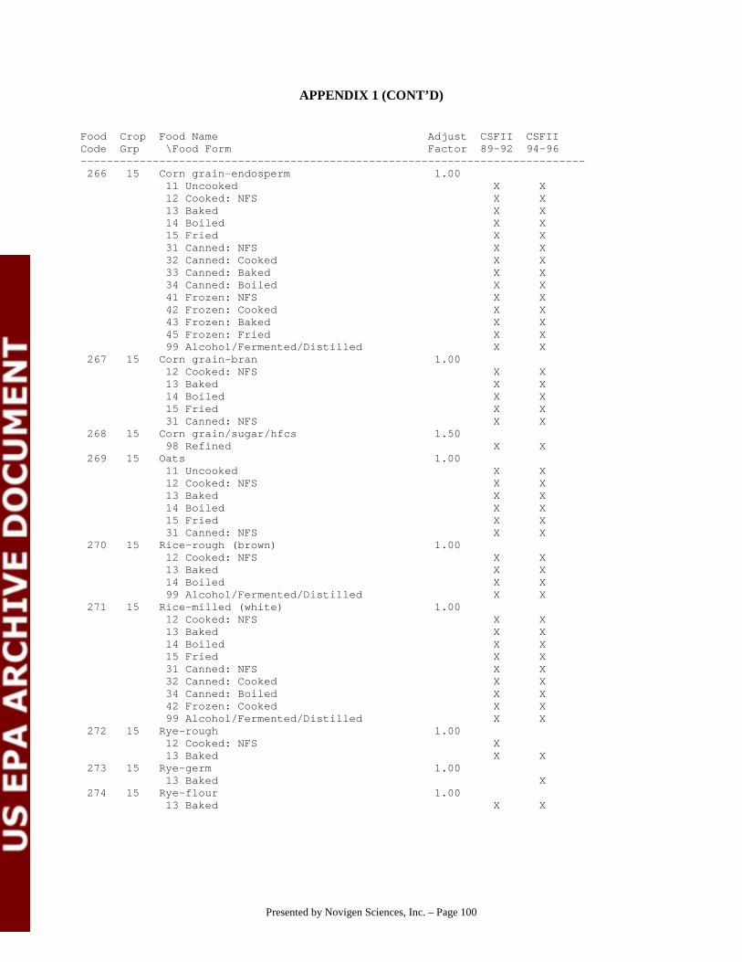
Presented by Novigen Sciences, Inc. – Page 100
APPENDIX 1 (CONT’D)
Food Crop Food Name Adjust CSFII CSFIICode Grp \Food Form Factor 89-92 94-96----------------------------------------------------------------------------- 266 15 Corn grain-endosperm 1.00 11 Uncooked X X 12 Cooked: NFS X X 13 Baked X X 14 Boiled X X 15 Fried X X 31 Canned: NFS X X 32 Canned: Cooked X X 33 Canned: Baked X X 34 Canned: Boiled X X 41 Frozen: NFS X X 42 Frozen: Cooked X X 43 Frozen: Baked X X 45 Frozen: Fried X X 99 Alcohol/Fermented/Distilled X X 267 15 Corn grain-bran 1.00 12 Cooked: NFS X X 13 Baked X X 14 Boiled X X 15 Fried X X 31 Canned: NFS X X 268 15 Corn grain/sugar/hfcs 1.50 98 Refined X X 269 15 Oats 1.00 11 Uncooked X X 12 Cooked: NFS X X 13 Baked X X 14 Boiled X X 15 Fried X X 31 Canned: NFS X X 270 15 Rice-rough (brown) 1.00 12 Cooked: NFS X X 13 Baked X X 14 Boiled X X 99 Alcohol/Fermented/Distilled X X 271 15 Rice-milled (white) 1.00 12 Cooked: NFS X X 13 Baked X X 14 Boiled X X 15 Fried X X 31 Canned: NFS X X 32 Canned: Cooked X X 34 Canned: Boiled X X 42 Frozen: Cooked X X 99 Alcohol/Fermented/Distilled X X 272 15 Rye-rough 1.00 12 Cooked: NFS X 13 Baked X X 273 15 Rye-germ 1.00 13 Baked X 274 15 Rye-flour 1.00 13 Baked X X

Presented by Novigen Sciences, Inc. – Page 101
APPENDIX 1 (CONT’D)
Food Crop Food Name Adjust CSFII CSFIICode Grp \Food Form Factor 89-92 94-96----------------------------------------------------------------------------- 275 15 Sorghum (including milo) 1.00 14 Boiled X 276 15 Wheat-rough 1.00 11 Uncooked X 12 Cooked: NFS X X 13 Baked X X 14 Boiled X X 277 15 Wheat-germ 1.00 12 Cooked: NFS X X 13 Baked X X 14 Boiled X X 278 15 Wheat-bran 1.00 11 Uncooked X X 12 Cooked: NFS X X 13 Baked X X 279 15 Wheat-flour 1.00 11 Uncooked X X 12 Cooked: NFS X X 13 Baked X X 14 Boiled X X 15 Fried X X 31 Canned: NFS X X 32 Canned: Cooked X X 33 Canned: Baked X X 34 Canned: Boiled X X 41 Frozen: NFS X X 42 Frozen: Cooked X X 43 Frozen: Baked X X 45 Frozen: Fried X X 52 Cured: Cooked(smokd/pickld/saltd) X X 280 15 Millet 1.00 13 Baked X X 281 O Honey 1.00 11 Uncooked X X 13 Baked X X 14 Boiled X X 15 Fried X X 34 Canned: Boiled X X 52 Cured: Cooked(smokd/pickld/saltd) X 282 1A Sugar-beet 1.00 98 Refined X X 283 O Sugar-cane 1.00 98 Refined X X 284 O Sugar-cane/molasses 1.00 13 Baked X X 285 O Maple sugar 1.00 14 Boiled X X 286 15 Buckwheat 1.00 12 Cooked: NFS X X 287 6C Guar beans 1.00 13 Baked X X 288 O Castor beans 1.00

Presented by Novigen Sciences, Inc. – Page 102
APPENDIX 1 (CONT’D)
Food Crop Food Name Adjust CSFII CSFIICode Grp \Food Form Factor 89-92 94-96----------------------------------------------------------------------------- 289 15 Corn grain-oil 1.00 98 Refined X X 290 O Cottonseed-oil 1.00 98 Refined X X 291 O Cottonseed-meal 1.00 13 Baked X X 292 O Flax seed 1.00 98 Refined X X 293 O Peanuts-oil 1.00 98 Refined X X 294 O Safflower-seed 1.00 295 O Safflower-oil 1.00 98 Refined X X 296 O Sesame-oil 1.00 98 Refined X X 297 6A Soybeans-oil 1.00 98 Refined X X 298 O Sunflower-oil 1.00 98 Refined X X 299 O Coconut-oil 1.00 98 Refined X X 300 O Olive oil 1.00 98 Refined X X 301 O Canola oil (rape seed oil) 1.00 98 Refined X X 302 O Palm oil 1.00 98 Refined X X 303 6A Soybean-other 1.00 304 6A Soybeans-mature seeds dry 1.00 12 Cooked: NFS X X 13 Baked X X 14 Boiled X X 15 Fried X X 41 Frozen: NFS X X 305 6A Soybeans-flour (full fat) 1.00 12 Cooked: NFS X X 13 Baked X 14 Boiled X X 34 Canned: Boiled X X 42 Frozen: Cooked X X 306 6A Soybeans-flour (low fat) 1.00 12 Cooked: NFS X X 13 Baked X X 15 Fried X X 31 Canned: NFS X X 307 6A Soybeans-flour (defatted) 1.00 12 Cooked: NFS X X 13 Baked X X 14 Boiled X X 15 Fried X X 31 Canned: NFS X X 34 Canned: Boiled X X

Presented by Novigen Sciences, Inc. – Page 103
APPENDIX 1 (CONT’D)
Food Crop Food Name Adjust CSFII CSFIICode Grp \Food Form Factor 89-92 94-96----------------------------------------------------------------------------- 42 Frozen: Cooked X X 98 Refined X X 308 O Oriental vegetables/non-leafy 1.00 309 O Seeds (misc.) 1.00 11 Uncooked X 13 Baked X X 14 Boiled X X 310 O Peppermint 1.00 311 O Peppermint-oil 1.00 14 Boiled X X 312 O Spearmint 1.00 313 O Spearmint-oil 1.00 314 O Vinegar 1.00 99 Alcohol/Fermented/Distilled X X 315 O Grapes-wine and sherry 1.00 99 Alcohol/Fermented/Distilled X X 316 O Alcohol-distilled 1.00 99 Alcohol/Fermented/Distilled X X 317 O Gelatin 1.00 12 Cooked: NFS X X 13 Baked X X 14 Boiled X X 41 Frozen: NFS X X 318 D Milk-nonfat solids 1.00 12 Cooked: NFS X X 13 Baked X X 14 Boiled X X 15 Fried X X 16 Pasteurized X X 18 Dried X X 31 Canned: NFS X X 32 Canned: Cooked X X 34 Canned: Boiled X X 41 Frozen: NFS X X 42 Frozen: Cooked X X 43 Frozen: Baked X X 45 Frozen: Fried X X 51 Cured: NFS (smoked/pickled/saltd) X X 52 Cured: Cooked(smokd/pickld/saltd) X X 98 Refined X 319 D Milk-fat solids 1.00 12 Cooked: NFS X X 13 Baked X X 14 Boiled X X 15 Fried X X 16 Pasteurized X X 18 Dried X X 31 Canned: NFS X X 32 Canned: Cooked X X 34 Canned: Boiled X X 41 Frozen: NFS X X 42 Frozen: Cooked X X

Presented by Novigen Sciences, Inc. – Page 104
APPENDIX 1 (CONT’D)
Food Crop Food Name Adjust CSFII CSFIICode Grp \Food Form Factor 89-92 94-96----------------------------------------------------------------------------- 45 Frozen: Fried X X 51 Cured: NFS (smoked/pickled/saltd) X X 52 Cured: Cooked(smokd/pickld/saltd) X X 320 D Milk sugar (lactose) 1.00 12 Cooked: NFS X X 13 Baked X X 14 Boiled X X 15 Fried X X 16 Pasteurized X X 18 Dried X X 31 Canned: NFS X X 32 Canned: Cooked X X 34 Canned: Boiled X X 41 Frozen: NFS X X 42 Frozen: Cooked X X 45 Frozen: Fried X X 51 Cured: NFS (smoked/pickled/saltd) X X 52 Cured: Cooked(smokd/pickld/saltd) X X 321 M Beef-meat byproducts 1.00 12 Cooked: NFS X X 52 Cured: Cooked(smokd/pickld/saltd) X X 322 M Beef-other organ meats 1.00 12 Cooked: NFS X X 14 Boiled X X 52 Cured: Cooked(smokd/pickld/saltd) X X 323 M Beef-dried 1.92 324 M Beef-fat w/o bones 1.00 11 Uncooked X 12 Cooked: NFS X X 13 Baked X X 14 Boiled X X 15 Fried X X 31 Canned: NFS X X 32 Canned: Cooked X X 34 Canned: Boiled X X 42 Frozen: Cooked X X 45 Frozen: Fried X X 51 Cured: NFS (smoked/pickled/saltd) X X 52 Cured: Cooked(smokd/pickld/saltd) X X 59 Cured: Dried (smokd/pickld/saltd) X X 325 M Beef-kidney 1.00 12 Cooked: NFS X 15 Fried X 326 M Beef-liver 1.00 12 Cooked: NFS X X 14 Boiled X X 15 Fried X X 327 M Beef-lean (fat/free) w/o bones 1.00 11 Uncooked X 12 Cooked: NFS X X 13 Baked X X 14 Boiled X X

Presented by Novigen Sciences, Inc. – Page 105
APPENDIX 1 (CONT’D)
Food Crop Food Name Adjust CSFII CSFIICode Grp \Food Form Factor 89-92 94-96----------------------------------------------------------------------------- 15 Fried X X 31 Canned: NFS X X 32 Canned: Cooked X X 33 Canned: Baked X X 34 Canned: Boiled X X 42 Frozen: Cooked X X 51 Cured: NFS (smoked/pickled/saltd) X X 52 Cured: Cooked(smokd/pickld/saltd) X X 59 Cured: Dried (smokd/pickld/saltd) X X 328 M Goat-meat byproducts 1.00 329 M Goat-other organ meats 1.00 330 M Goat-fat w/o bone 1.00 13 Baked X X 14 Boiled X X 331 M Goat-kidney 1.00 332 M Goat-liver 1.00 333 M Goat-lean (fat/free) w/o bone 1.00 13 Baked X X 14 Boiled X X 334 M Horsemeat 1.00 335 M Rabbit 1.00 12 Cooked: NFS X X 336 M Sheep-meat byproducts 1.00 337 M Sheep-other organ meats 1.00 338 M Sheep-fat w/o bone 1.00 12 Cooked: NFS X X 13 Baked X X 14 Boiled X X 31 Canned: NFS X X 52 Cured: Cooked(smokd/pickld/saltd) X X 339 M Sheep-kidney 1.00 340 M Sheep-liver 1.00 341 M Sheep-lean (fat free) w/o bone 1.00 12 Cooked: NFS X X 13 Baked X X 14 Boiled X X 15 Fried X X 342 M Pork-meat byproducts 1.00 12 Cooked: NFS X X 14 Boiled X X 15 Fried X X 52 Cured: Cooked(smokd/pickld/saltd) X X 343 M Pork-other organ meats 1.00 12 Cooked: NFS X X 15 Fried X X 344 M Pork-fat w/o bone 1.00 11 Uncooked X 12 Cooked: NFS X X 13 Baked X X 14 Boiled X X 15 Fried X X 31 Canned: NFS X X

Presented by Novigen Sciences, Inc. – Page 106
APPENDIX 1 (CONT’D)
Food Crop Food Name Adjust CSFII CSFIICode Grp \Food Form Factor 89-92 94-96----------------------------------------------------------------------------- 32 Canned: Cooked X X 34 Canned: Boiled X X 42 Frozen: Cooked X X 51 Cured: NFS (smoked/pickled/saltd) X X 52 Cured: Cooked(smokd/pickld/saltd) X X 60 Canned: Cured X X 345 M Pork-kidney 1.00 346 M Pork-liver 1.00 12 Cooked: NFS X X 15 Fried X X 347 M Pork-lean (fat free) w/o bone 1.00 12 Cooked: NFS X X 13 Baked X X 14 Boiled X X 15 Fried X X 31 Canned: NFS X X 32 Canned: Cooked X X 34 Canned: Boiled X X 42 Frozen: Cooked X X 51 Cured: NFS (smoked/pickled/saltd) X X 52 Cured: Cooked(smokd/pickld/saltd) X X 60 Canned: Cured X X 349 F Fish-shellfish 1.00 11 Uncooked X X 12 Cooked: NFS X X 13 Baked X X 14 Boiled X X 15 Fried X X 31 Canned: NFS X X 32 Canned: Cooked X X 34 Canned: Boiled X X 35 Canned: Fried X X 51 Cured: NFS (smoked/pickled/saltd) X X 350 O Meat-game 1.00 12 Cooked: NFS X X 13 Baked X X 14 Boiled X X 51 Cured: NFS (smoked/pickled/saltd) X 59 Cured: Dried (smokd/pickld/saltd) X X 351 F Fish-roe/caviar 1.00 11 Uncooked X X 352 F Fish-finfish/freshwater 1.00 12 Cooked: NFS X X 13 Baked X X 14 Boiled X X 15 Fried X X 51 Cured: NFS (smoked/pickled/saltd) X X 353 F Fish-finfish/saltwater (incl. tuna) 1.00 11 Uncooked X X 12 Cooked: NFS X X 13 Baked X X 14 Boiled X X

Presented by Novigen Sciences, Inc. – Page 107
APPENDIX 1 (CONT’D)
Food Crop Food Name Adjust CSFII CSFIICode Grp \Food Form Factor 89-92 94-96----------------------------------------------------------------------------- 15 Fried X X 31 Canned: NFS X X 32 Canned: Cooked X X 33 Canned: Baked X X 34 Canned: Boiled X X 35 Canned: Fried X X 42 Frozen: Cooked X X 51 Cured: NFS (smoked/pickled/saltd) X X 59 Cured: Dried (smokd/pickld/saltd) X 354 F Fish-finfish-saltwater-dried 1.60 18 Dried X 59 Cured: Dried (smokd/pickld/saltd) X 355 P Turkey-byproducts 1.00 12 Cooked: NFS X X 34 Canned: Boiled X X 42 Frozen: Cooked X X 52 Cured: Cooked(smokd/pickld/saltd) X X 356 P Turkey-giblets (liver) 1.00 12 Cooked: NFS X X 357 P Turkey--fat w/o bones 1.00 12 Cooked: NFS X X 13 Baked X X 14 Boiled X X 15 Fried X X 31 Canned: NFS X X 32 Canned: Cooked X X 34 Canned: Boiled X X 42 Frozen: Cooked X X 51 Cured: NFS (smoked/pickled/saltd) X X 52 Cured: Cooked(smokd/pickld/saltd) X X 358 P Turkey- lean/fat free w/o bones 1.00 12 Cooked: NFS X X 13 Baked X X 14 Boiled X X 15 Fried X X 31 Canned: NFS X X 32 Canned: Cooked X X 34 Canned: Boiled X X 42 Frozen: Cooked X X 51 Cured: NFS (smoked/pickled/saltd) X X 52 Cured: Cooked(smokd/pickld/saltd) X X 360 P Poultry-other-lean (fat free) w/o bone 1.00 12 Cooked: NFS X X 13 Baked X X 361 P Poultry-other-giblets(liver) 1.00 362 P Poultry-other-fat w/o bones 1.00 12 Cooked: NFS X X 13 Baked X X 14 Boiled X X 363 P Eggs-whole 1.00 11 Uncooked X X 12 Cooked: NFS X X

Presented by Novigen Sciences, Inc. – Page 108
APPENDIX 1 (CONT’D)
Food Crop Food Name Adjust CSFII CSFIICode Grp \Food Form Factor 89-92 94-96----------------------------------------------------------------------------- 13 Baked X X 14 Boiled X X 15 Fried X X 31 Canned: NFS X X 34 Canned: Boiled X X 41 Frozen: NFS X X 42 Frozen: Cooked X X 45 Frozen: Fried X X 364 P Eggs-white only 1.00 11 Uncooked X 12 Cooked: NFS X X 13 Baked X X 14 Boiled X X 31 Canned: NFS X X 32 Canned: Cooked X X 34 Canned: Boiled X X 41 Frozen: NFS X X 42 Frozen: Cooked X X 365 P Eggs-yolk only 1.00 11 Uncooked X X 12 Cooked: NFS X X 13 Baked X X 14 Boiled X X 15 Fried X X 31 Canned: NFS X X 32 Canned: Cooked X X 34 Canned: Boiled X X 41 Frozen: NFS X X 366 P Chicken-byproducts 1.00 12 Cooked: NFS X X 34 Canned: Boiled X X 367 P Chicken-giblets(liver) 1.00 12 Cooked: NFS X X 13 Baked X 15 Fried X X 42 Frozen: Cooked X 368 P Chicken-fat w/o bones 1.00 12 Cooked: NFS X X 13 Baked X X 14 Boiled X X 15 Fried X X 31 Canned: NFS X X 32 Canned: Cooked X X 34 Canned: Boiled X X 42 Frozen: Cooked X X 369 P Chicken-lean/fat free w/o bones 1.00 12 Cooked: NFS X X 13 Baked X X 14 Boiled X X 15 Fried X X 31 Canned: NFS X X 32 Canned: Cooked X X

Presented by Novigen Sciences, Inc. – Page 109
APPENDIX 1 (CONT’D)
Food Crop Food Name Adjust CSFII CSFIICode Grp \Food Form Factor 89-92 94-96----------------------------------------------------------------------------- 34 Canned: Boiled X X 42 Frozen: Cooked X X 376 O Aloe vera-juice 1.00 11 Uncooked X 377 11 Apples-juice-concentrate 3.90 12 Cooked: NFS X X 13 Baked X X 31 Canned: NFS X X 41 Frozen: NFS X X 378 O Bananas-juice 1.00 11 Uncooked X X 31 Canned: NFS X X 379 1A Sugar-beet-molasses 1.00 98 Refined X 380 13A Blackberries-juice 1.00 11 Uncooked X X 31 Canned: NFS X X 381 19B Pepper/black 1.00 11 Uncooked X X 12 Cooked: NFS X X 13 Baked X X 14 Boiled X X 15 Fried X X 31 Canned: NFS X X 32 Canned: Cooked X X 42 Frozen: Cooked X X 52 Cured: Cooked(smokd/pickld/saltd) X X 382 1AB Burdock 1.00 12 Cooked: NFS X 383 5B Cabbage-savoy 1.00 12 Cooked: NFS X 384 4B Celery juice 1.00 31 Canned: NFS X X 385 P Chicken-giblets (excl. liver) 1.00 12 Cooked: NFS X X 14 Boiled X X 34 Canned: Boiled X X 42 Frozen: Cooked X 386 9B Christophine 1.00 387 O Coconut-milk 1.00 11 Uncooked X X 12 Cooked: NFS X X 31 Canned: NFS X X 388 15 Corn grain/sugar-molasses 1.50 12 Cooked: NFS X X 41 Frozen: NFS X X 389 O Cranberries-juice-concentrate 3.30 31 Canned: NFS X X 390 O Fern shoots (fiddleheads) 1.00 392 O Grapes-juice-concentrate 3.60 12 Cooked: NFS X X 13 Baked X X

Presented by Novigen Sciences, Inc. – Page 110
APPENDIX 1 (CONT’D)
Food Crop Food Name Adjust CSFII CSFIICode Grp \Food Form Factor 89-92 94-96----------------------------------------------------------------------------- 14 Boiled X X 31 Canned: NFS X X 41 Frozen: NFS X X 393 O Guava-juice 1.00 31 Canned: NFS X 394 O Jackfruit 1.00 395 O Jobo 1.00 396 O Lotus root 1.00 14 Boiled X X 397 9B Okra/chinese (luffa) 1.00 398 D Milk-based water 1.00 12 Cooked: NFS X X 13 Baked X X 14 Boiled X X 15 Fried X X 16 Pasteurized X X 18 Dried X X 31 Canned: NFS X X 32 Canned: Cooked X X 33 Canned: Baked X X 34 Canned: Boiled X X 41 Frozen: NFS X X 42 Frozen: Cooked X X 43 Frozen: Baked X X 45 Frozen: Fried X X 52 Cured: Cooked(smokd/pickld/saltd) X X 399 15 Oats-bran 1.00 11 Uncooked X X 12 Cooked: NFS X 13 Baked X X 14 Boiled X X 15 Fried X 400 O Palm hearts 1.00 14 Boiled X X 401 O Passion fruit-juice 1.00 11 Uncooked X X 12 Cooked: NFS X X 14 Boiled X X 31 Canned: NFS X X 402 12 Peaches-juice 1.00 11 Uncooked X X 31 Canned: NFS X X 403 O Peanuts-butter 1.89 13 Baked X X 14 Boiled X X 404 11 Pears-juice 1.00 11 Uncooked X X 12 Cooked: NFS X X 13 Baked X X 31 Canned: NFS X X 33 Canned: Baked X X 41 Frozen: NFS X
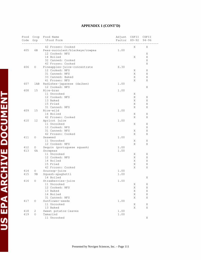
Presented by Novigen Sciences, Inc. – Page 111
APPENDIX 1 (CONT’D)
Food Crop Food Name Adjust CSFII CSFIICode Grp \Food Form Factor 89-92 94-96----------------------------------------------------------------------------- 42 Frozen: Cooked X X 405 6B Peas-succulent/blackeye/cowpea 1.00 12 Cooked: NFS X 14 Boiled X X 32 Canned: Cooked X 42 Frozen: Cooked X 406 O Pineapples-juice-concentrate 6.30 12 Cooked: NFS X X 31 Canned: NFS X X 33 Canned: Baked X X 41 Frozen: NFS X X 407 1AB Radishes-japanese (daiken) 1.00 12 Cooked: NFS X 408 15 Rice-bran 1.00 11 Uncooked X 12 Cooked: NFS X X 13 Baked X X 15 Fried X X 31 Canned: NFS X X 409 15 Rice-wild 1.00 14 Boiled X X 42 Frozen: Cooked X X 410 12 Apricot juice 1.00 11 Uncooked X X 12 Cooked: NFS X 31 Canned: NFS X X 42 Frozen: Cooked X X 411 O Seaweed 1.00 11 Uncooked X X 12 Cooked: NFS X X 412 O Sequin (portuguese squash) 1.00 413 6A Snowpeas 1.00 11 Uncooked X X 12 Cooked: NFS X X 14 Boiled X X 15 Fried X X 42 Frozen: Cooked X X 414 O Soursop-juice 1.00 415 9B Squash-spaghetti 1.00 14 Boiled X 416 O Strawberries-juice 1.00 11 Uncooked X X 12 Cooked: NFS X X 13 Baked X X 14 Boiled X X 31 Canned: NFS X X 417 O Sunflower-seeds 1.00 11 Uncooked X X 13 Baked X X 418 2 Sweet potatos-leaves 1.00 419 O Tamarind 1.00 11 Uncooked X

Presented by Novigen Sciences, Inc. – Page 112
APPENDIX 1 (CONT’D)
Food Crop Food Name Adjust CSFII CSFIICode Grp \Food Form Factor 89-92 94-96----------------------------------------------------------------------------- 420 10 Tangerines-juice-concentrate 7.35 422 O Thistle leaves 1.00 423 8 Tomatoes-dried 14.30 12 Cooked: NFS X 15 Fried X 424 M Veal-fat w/o bones 1.00 12 Cooked: NFS X X 13 Baked X X 14 Boiled X X 15 Fried X X 31 Canned: NFS X 425 M Veal-lean (fat free) w/o bones 1.00 12 Cooked: NFS X X 13 Baked X X 14 Boiled X X 15 Fried X X 31 Canned: NFS X 426 M Veal-kidney 1.00 15 Fried X 427 M Veal-liver 1.00 14 Boiled X 428 M Veal-other organ meats 1.00 429 M Veal-dried 1.92 430 M Veal-meat byproducts 1.00 431 14 Walnut oil 1.00 432 O Water-bottled 1.00 433 O Water-tap 1.00 11 Uncooked X X 12 Cooked: NFS X X 13 Baked X X 14 Boiled X X 15 Fried X X 434 O Water-commercial processing 1.00 11 Uncooked X X 12 Cooked: NFS X X 13 Baked X X 14 Boiled X X 15 Fried X X 16 Pasteurized X X 18 Dried X X 31 Canned: NFS X X 32 Canned: Cooked X X 33 Canned: Baked X X 34 Canned: Boiled X X 35 Canned: Fried X X 41 Frozen: NFS X X 42 Frozen: Cooked X X 43 Frozen: Baked X X 44 Frozen: Boiled X 51 Cured: NFS (smoked/pickled/saltd) X X 52 Cured: Cooked(smokd/pickld/saltd) X X 60 Canned: Cured X X

Presented by Novigen Sciences, Inc. – Page 113
APPENDIX 1 (CONT’D)
Food Crop Food Name Adjust CSFII CSFIICode Grp \Food Form Factor 89-92 94-96----------------------------------------------------------------------------- 98 Refined X X 435 O Water-non-food based 1.00 436 9A Watermelon-juice 1.00 437 15 Wheat-germ oil 1.00 13 Baked X X 438 O Wi-apple 1.00 439 9B Wintermelon 1.00 14 Boiled X 440 O Yeast 1.00 12 Cooked: NFS X X 99 Alcohol/Fermented/Distilled X X 441 10 Grapefruit-juice-concentrate 8.26 41 Frozen: NFS X X 442 10 Lemons-juice-concentrate 11.40 12 Cooked: NFS X X 13 Baked X X 14 Boiled X X 31 Canned: NFS X X 34 Canned: Boiled X X 41 Frozen: NFS X X 443 10 Limes-juice-concentrate 6.00 12 Cooked: NFS X X 41 Frozen: NFS X X 447 4A Chervil 1.00 14 Boiled X X 448 10 Grapefruit peel 1.00 449 P Turkey-other organ meats 1.00 12 Cooked: NFS X X 450 1AB Ginseng 1.00 11 Uncooked X 451 5A Broccoli-chinese 1.00 14 Boiled X X 452 5B Bok choy 1.00 11 Uncooked X X 12 Cooked: NFS X X 14 Boiled X X 42 Frozen: Cooked X X 51 Cured: NFS (smoked/pickled/saltd) X X 460 O Seafood-misc(turtle/frog) 1.00 12 Cooked: NFS X 14 Boiled X X 467 19B Celery seed 1.00 11 Uncooked X X 14 Boiled X X 31 Canned: NFS X X 51 Cured: NFS (smoked/pickled/saltd) X X 473 O Sapodilla 1.00 480 O Plantains-green 1.00 15 Fried X 481 O Plantains-dried 3.90 482 O Soybeans-protein isolate 1.00 12 Cooked: NFS X X

Presented by Novigen Sciences, Inc. – Page 114
APPENDIX 1 (CONT’D)
Food Crop Food Name Adjust CSFII CSFIICode Grp \Food Form Factor 89-92 94-96----------------------------------------------------------------------------- 13 Baked X X 14 Boiled X X 15 Fried X X 31 Canned: NFS X X 32 Canned: Cooked X X 33 Canned: Baked X X 34 Canned: Boiled X X 41 Frozen: NFS X X 42 Frozen: Cooked X X 51 Cured: NFS (smoked/pickled/saltd) X 483 O Chayote 1.00 484 O Radishes-oriental 1.00 485 O Leaves (misc) 1.00 11 Uncooked X 14 Boiled X X 31 Canned: NFS X X 34 Canned: Boiled X X 489 O Vanilla 1.00 99 Alcohol/Fermented/Distilled X X 491 O Arugula 1.00 11 Uncooked X 492 O Radicchio 1.00 11 Uncooked X 493 O Tarragon 1.00 14 Boiled X X 494 O Saffron 1.00 14 Boiled X X 495 O Cilantro 1.00 11 Uncooked X 12 Cooked: NFS X 496 O Nopales 1.00 11 Uncooked X 14 Boiled X X 497 9B Balsam pear 1.00 498 4A Amaranth 1.00 13 Baked X X 890 O Miscellaneous/nfs 1.00 11 Uncooked X X 12 Cooked: NFS X X 13 Baked X X 14 Boiled X X 15 Fried X X 31 Canned: NFS X X 32 Canned: Cooked X X 33 Canned: Baked X X 34 Canned: Boiled X X 41 Frozen: NFS X X 42 Frozen: Cooked X X 51 Cured: NFS (smoked/pickled/saltd) X X 52 Cured: Cooked(smokd/pickld/saltd) X X 60 Canned: Cured X X

Presented by Novigen Sciences, Inc. – Page 115
APPENDIX 1 (CONT’D)
Food Crop Food Name Adjust CSFII CSFIICode Grp \Food Form Factor 89-92 94-96----------------------------------------------------------------------------- 891 O Jute 1.00 892 O Chrysanthemum 1.00 893 O Salt 1.00 98 Refined X X 894 O Leavening agents 1.00 12 Cooked: NFS X X 895 O Psyllium 1.00 13 Baked X X 896 O Sweeteners-artificial 1.00 12 Cooked: NFS X X 897 O Gums/gels 1.00 11 Uncooked X X 12 Cooked: NFS X X 13 Baked X X 14 Boiled X X 15 Fried X X 31 Canned: NFS X X 32 Canned: Cooked X X 34 Canned: Boiled X X 41 Frozen: NFS X X 42 Frozen: Cooked X X 911 O Molasses-nfs 1.00 98 Refined X X 940 O Peanuts-hulled 1.00 12 Cooked: NFS X X 13 Baked X X 14 Boiled X X 15 Fried X X 41 Frozen: NFS X X 950 O Beer 1.00 99 Alcohol/Fermented/Distilled X X

Presented by Novigen Sciences, Inc. – Page 116
Appendix 2
Algorithm Documentation for the DEEM™ Acuteand Chronic Program Modules

Presented by Novigen Sciences, Inc. – Page 117
Algorithm Documentation for the DEEM™ Acuteand Chronic Program Modules*
By:Stephen R. Petersen
Durango Software, LLC
Presented to:The Advanced DEEM™ Users Workshop
Washington, DC
January 18, 2000
* Copyright 2000 by Durango Software LLC. All rights reserved. Reproduction prohibited except by written permission fromDurango Software LLC.

Copyright 2000 by Durango Software LLC. All rights reserved. Reproduction prohibited except by written permission from Durango SoftwareLLC.
Presented by Novigen Sciences, Inc. – Page 118
Algorithm Documentation for the DEEM™ Acuteand Chronic Program Modules
By Stephen R. Petersen, Durango Software, LLC
The Novigen Sciences Dietary Exposure and Evaluation Model (DEEM™), written in Visual Basic for IBM-compatible personal computers by Durango Software LLC, consists of four executable modules: The main DEEM™module, the Acute analysis module, the Chronic analysis module, and the RDFgen™ module. The main DEEM™module is used by the exposure analyst to create and edit residue files for specific chemical application, to launch theseparate DEEM™ Acute, Chronic and RDFgen™ modules, and to specify file directories and certain report formattingoptions. This documentation focuses on the computational algorithms in the two analytical modules. User-createdDEEM™ residue files are self-documenting. That is, both the residue file itself and an annotated version of the file(for inclusion with a completed DEEM™ analysis) can be printed or displayed to the screen for visual inspection andverification. The RDFgen™ module also produces self documented files.
Before undertaking either a DEEM™ Acute or DEEM™ Chronic analysis, the user must prepare a chemical-specificresidue file, using the DEEM™ residue file editor, in which default chemical residue amounts, residue distributionfunctions, and adjustment factors are set up for each food or food/foodform of interest, along with the toxicologyendpoints (separately for chronic and acute analyses) to be used in the analyses. The same DEEM™ residue file can beused by both the DEEM™ Chronic and DEEM™ Acute modules for the analysis of a given chemical, as well as by theNovigen Sciences Calendex™ program for computing dietary exposure in an aggregate or cumulative exposure.(Toxicology endpoints can be changed at the time that the analyses are launched.) The validity of the Acute and/orChronic analyses for a given chemical is largely determined by the quality of the data in the residue file used in theanalysis. (The GIGO principle.) The Acute and Chronic modules apply the residue data in the residue files (and insupporting residue distribution files) to food consumption data derived from the USDA’s Continuing Survey of FoodIntakes by Individuals (CSFII) to determine acute and chronic exposure amounts in the U.S. Population and specifiedsubsets of that population. The validity of the DEEM™ Acute and Chronic analyses for a given chemical is largelydetermined by the quality of the data in the residue file used in those analyses. (The GIGO principle.)
Guide to this documentation
A. The Acute Exposure Module page 1191. Variables used in Acute analysis page 1192. Important constants used in the acute analysis module page 1203. Ten steps in the Acute Analysis page 1214. Subroutine ComputeExpos page 1235. Acute module code segments page 1266. Subroutines used to compute
distributions from distribution parameters page 136
B. The Chronic Exposure module page 1381. Steps in a Chronic Analysis page 1392. Non-Food-Based (NFB) Water
consumption means page 1423. Subroutine to calculate body weight for CSFII participants
who do not have a recorded bodyweight page 143
C. The RDFgen™ Module Page 145

Copyright 2000 by Durango Software LLC. All rights reserved. Reproduction prohibited except by written permission from Durango SoftwareLLC.
Presented by Novigen Sciences, Inc. – Page 119
A. The Acute Exposure Module
1. Variables used in the Acute analysis module
User specifies the following variables to be used in an Acute analysis:
Variable TypeResidue file name (*.R96 or *.RS7)Divide Exposure by Body Weight bw Boolean (0,1)Use second adjustment factor usesecond Boolean (0,1)Use Monte Carlo Analysis (MCA) flagmc Boolean (0,1)Generate CEC file CEC Boolean (0,1)Evaluate foods by eating occasion lineitem Boolean (0,1)Number of Standard Pops to be evaluated npops integer 1-27Standard populations to be evaluated popx (1 to 27) Boolean (0,1)Number of Custom Pops to be evaluated nsubpops integer 1-6List of custom populations isubpop (1 to 6) Boolean (0,1)NFCS survey to be used survey 1 = 1989-91; 2 = 1994-96
If MCA is used:number of iterations nsims integer 1 to 5000random number seed seed integer 1 to 32,000
If CEC file is to be generated:Number of printed records nrecordstosave integer 1 0 500Minimum exposure contribution
by food/foodform cecminperc! Real 1 to 100Excel format ExcelOption Boolean (0,1)Low percentile boundary LowPctl! Real .95 to .999High percentile boundary HighPctl! Real .95 to 1.0
The current residue file defines the list of residue distribution functions in general and specific default residue values,adjustment factors, and (optionally) residue distribution pointers and ratios for each food/foodform to be include in thecurrent analysis.
All valid food (RAC) and Foodform codes are shown in the DEEM™ residue file editor with their correspondingnames. RAC codes are assigned to all foods (integer 1-950, but not all numbers in this series are used.)Foodform codes are assigned to all foods which are actually consumed in either CSFII survey (integer 11-99, but notall numbers are used.)
Active foodforms for any consumed food (RAC) were predetermined at the time that Novigen recipe translation factorswere initially applied to the CSFII foods “as-eaten” for all participants in preparing the Acute food consumption database; only those food/foodform combinations that are derived from the foods “as eaten” either survey (CSFII 1989-91or 1994-96) are considered “active”. Note that food/foodform consumption records in the Acute data base werecalculated for each individual separately, and that the total daily consumption amount for each food/foodform for eachindividual was rounded to the nearest 0.1g before it was saved to the Acute data base. (By multiplying the dailyconsumption amount for each food/foodform by 10 the resulting amount could be saved as an integer instead of a realnumber, which halved the data storage requirement for this large data base. The conversion of the food consumptionvalues in the data base back to 0. 1 g is performed as part of the Acute analysis.) Note that in the “line item” data baseof individual food consumption for Acute analysis by eating occasion, each occurrence of food/foodform consumptionis rounded to 0.1 g, multiplied by 10, and saved separately as an integer amount rather than combining them into adaily total. In both the daily total food consumption data base and the line-item food consumption data base used in theAcute analysis module, food/foodform consumption amounts represent intake amounts by individuals unadjusted forbody weight.

Copyright 2000 by Durango Software LLC. All rights reserved. Reproduction prohibited except by written permission from Durango SoftwareLLC.
Presented by Novigen Sciences, Inc. – Page 120
If survey = 1 (CSFII 89-91) then nregions = 9 (CSFII 89-91 uses 9 census regions) ndays = 3 (Number of days in survey) k1 = 458 (Number of foods (RACs) k2 = 1264 (Number of food/food form combinations, plus nfb water) k4 = 27 (Number of standard populations, including pacific census region)
If survey = 2 (CSFII 94-96) nregions = 4 (CSFII 94-96 uses 4 census regions) ndays = 2 (Number of days in survey) k1 = 458 (Number of foods (RACs) k2 = 1270 (Number of food/food form combinations, plus nfb water) k4 = 26 (Number of standard populations, (Pacific is not available due to limitation on census regions)
Other variables and arrays needed in the analysis:RacIndex(rac) = array with RAC indices as function of RACs (k1 indices )NSI(rac index) = array with RACs as function of rac indices (reverse of RacIndex array)Ffcd(1-k2) is array with active foodform codes for each RACFFF(1-k1) is array with location in Ffcd() of first foodform available for each RAC (as indexed)NFF(1-k1) is array with number of food forms in Ffcd() available for each RAC (as indexed)waterindex = 415 (the rac index for nfb water, which is not included directly in the CSFII food consumption records)k7 = number of standard populations (npops) + number of custom populations (nsubpops) selected for analysis in thecurrent run.
Programming conventions:All variable and array names ending with “!” are real numbers (7 significant digits).All variable and array names ending with “&” are long integers.All variable and array names ending with “#” are double-precision real numbers (14 significant digits).All variables and array names ending with “$” are strings.All variable names ending without a special character areintegers (0-32,767).
2. Important constants used in the acute analysis module:
Percentile markers:pctl!(0) = 100 pctl!(1) = 90pctl!(2) = 80 pctl!(3) = 70pctl!(4) = 60 pctl!(5) = 50pctl!(6) = 40 pctl!(7) = 30pctl!(8) = 20 pctl!(9) = 10pctl!(10) = 5 pctl!(11) = 2.5pctl!(12) = 1 pctl!(13) = 0.5pctl!(14) = 0.25 pctl!(15) = 0.1
Standard Populations:1 U.S. Pop - 48 states - all seasons2 U.S. Population - spring season3 U.S. Population - summer season4 U.S. Population - autumn season5 U.S. Population - winter season6 Northeast region7 Midwest region8 Southern region9 Western region10 Hispanics11 Non-hispanic whites

Copyright 2000 by Durango Software LLC. All rights reserved. Reproduction prohibited except by written permission from Durango SoftwareLLC.
Presented by Novigen Sciences, Inc. – Page 121
12 Non-hispanic blacks13 Non-hispanic other than black or white14 All infants (<1 year)15 Nursing infants (<1 year)16 Non-nursing infants (<1 year)17 Children (1-6 years)18 Children (7-12 years)19 Females (13+/pregnant/not nursing)20 Females (13+/nursing)21 Females (13-19 yrs/not preg. or nursing)22 Females (20+ years/not preg. or nursing)23 Females (13-50 years)24 Males (13-19 years)25 Males (20+ years)26 Seniors (55+)27 Pacific Region (Used only in CSFII 1989-91 analyses)
3. Ten steps in the Acute Analysis:
Step 1: Read in the residue file to be used in this analysis(1) Read in distribution functions (i = 1 to Nindices) ResDistType(i) = residue distribution type (0-6) of ith function (see list of distribution types and parameters) ResParam!(i, j) = jth residue parameter for ith residue distribution function (j = 1 to 3) McFl$(i) = name of RDF file if ith residue distribution type = 6(2) Read in residue amounts, conversion factors, distribution pointers and probabilities ratios Tol!(i) = residue amount for ith Rac in residue file (i = 1 to totalfoods)
Cf!(i) = conversion factor #1 for ith food Cf2!(i) = conversion factor #2 for ith food Rff(i) = number of food forms included in the residue file for this RAC DistPointer(i,j) = jth distribution index for ith RAC (j = 1 to 5) DistRatio!(i,j) = jth distribution probability ratio for ith RAC (j = 1 to 5) (must add to 1.0) FFTol!(l) = residue amount for food form FFF(l) FFCf!(l) = conversion factor #1 for food form FFF(l) FFCf2!(l) = conversion factor #2 for food form FFF(l) FFDistPointer(l,j) = jth distribution index for lth food form (j = 1 to 5) FFDistRatio!(l,j) = jth distribution probability ratio for lth food form (j = 1 to 5) (must add to 1.0)
Step 2: For any RAC without foodforms, convert RACs to its constituent food forms (analysis is never performed atRAC level because all food consumption amounts in the Acute food consumption data base are stored at the foodformlevel.
See code segment #1
Step 3: (MCA with RDFs only) Preprocess all residue distribution file (RDF) declared in the current residue file andsave results to two temporary files. (1) The first contains summary statistics for each RDF file, including the number ofdeclared zeros/, the number of declared LODs (limit of detection), the LOD residue value, the number of specifiedresidue values, and a location variable showing the starting address of its corresponding list of specified residue valuesin the second file. (2) The second file contains a vector of the individually specified residue values for all of the RDFfiles declared in the residue file.
Step 4: (MCA only) Compute ffmcmean!, CumProb!, and wtdmeanff! Arrays for use in MCA.The ffmcmean! array is the approximate mean value that will be returned from any given residue distribution function(not including the declared zeros in the case of an RDF file). It is computed in subroutine rdfmeans. Note that theapproximate mean for distribution types 2-5 is found by sampling the referenced distribution with random samplingvalues of 0.05, 0.15, …0.95, summing these values and then dividing by 10 (an exact value is not needed; these means

Copyright 2000 by Durango Software LLC. All rights reserved. Reproduction prohibited except by written permission from Durango SoftwareLLC.
Presented by Novigen Sciences, Inc. – Page 122
will be used to estimate the mean exposure amount for each population which in turn will be used to calibrate the binsfor capturing the exposure distribution.See code segment #2
The CumProb! array is the cumulative probability of use (real, 0 to 1) for each of up to 5 different residue distributionfunctions specified for a given food/foodform in the current residue file. The cumulative probability is based on theindividual probabilities assigned to each function (which must add up to 1.0) and the order in which they are includedin the residue file for that food/foodform. See code segment #3.
The wtdmeanff! array is the weighted mean for each food/foodform based on the 1 to 5 RDF’s specified for that usingone or more residue distribution functions and cumulative probability of each rdf used with each foodform). See codesegment #3.
Step 5: Compute FFFactor! array of preliminary exposure calculations for each food/foodform having a definedresidue in the current residue file. If MCA is not used, or there is no RDL pointer for the lth food/food form, thenFFFactor!(l) (l here is lower case letter L) is the residue amount, multiplied by the adjustment factors, that can bemultiplied by individual food/foodform consumption amounts to yield individual exposure for that food/foodform. IfMCA is used and one or more RDL pointers are used for any given food/foodform, then FFFactor!(l) represents theadjustment factors only; the residue amount must be determined probabilistically from the appropriate residuedistribution function. If a food/foodform is not included in the residue file, then FFFactor!(l) = 0.
See code segment #4.
Step 6: First pass through entire food consumption data base to compute the approximate mean daily exposure forusers (participants who consume at least one of the food/foodforms in the residue file) in each population groupspecified when setting up the analysis. These means will be used to set up the exposure bins needed for distributionanalysis.
Residue selection: If this is not an MCA, the default (deterministic) residues amounts for each food/foodform in theresidue file are used in computing individual exposure amounts. If this is an MCA, then the mean residue amounts foreach food/foodform, as derived from the residue distribution functions (wtdmeanff!(1 to k2)) in the residue file, areused. However, in the first pass only a single iteration is performed and no stochastic processes (using randomnumbers) are employed.
Set testmean = 1.
Then call the computeexpos subroutine to compute mean daily exposure for the users in each populationReturn with array cmeans!(i), i = 1 to number of populations to be evaluated (including both standard populations(npops) and custom populations (nsubpops)). Set scalar! array = Cmeans! array. ComputeExpos subroutine shownbelow.
Step 7: (only used when generating CEC file): Make a pass through the entire food consumption data base with 10iterations (if MCA) or 1 iteration (if no MCA) to determine the approximate user exposure at the 95th percentile foreach population selected.
Set CEC =1, testmean = 0, and Nsims (number of MC iterations) = 10Call subroutine computeexposReturn with distribution array, ex#():Call distribution subroutine with Ex# array to find daily exposure at 95th percentile for each selected population (1-k7)and place in Array cecvalue!(k7).
Step 8: Call ComputeExpos to determine the total daily exposure for each individual on each day in the survey andplace this exposure amount into the bin vector, bin&(), for each population. Also generate the summation variablesneeded to compute mean, standard deviation, and standard error of mean for each population.

Copyright 2000 by Durango Software LLC. All rights reserved. Reproduction prohibited except by written permission from Durango SoftwareLLC.
Presented by Novigen Sciences, Inc. – Page 123
If this total daily exposure exceeds the preliminary exposure estimate at the 95th percentile, as determined in step 7,save a record of this individual’s demographic variables (age, sex, body weight) and daily exposure amount,along witha list of the food/foodforms eaten that contribute to this exposure amount, including their consumption amount, residueamount, and adjustment factors. Individual foods/foodforms are only included in this list if their percentagecontribution to the total daily exposure exceeds the percentage level specified by the user (“minimum exposurecontribution by food”). These CEC records are is saved to a temporary disk file which is post-processed after the finalacute exposure analysis report is generated.
Step 9: Call the report subroutine to generate the acute analysis report, which contains user and per capita means,standard deviation, and standard error or mean, as well as exposure distributions for users and per capita, for alldesignated populations.
For each population of interest, i (1 to k7), compute the percent of total person-days in the survey that are user days(i.e., at least one of the food/foodform combinations in the residue file were eaten)
See code segment #14
For both users and per capita, compute:(1) the mean exposure: See code segment #15(2) standard deviation and standard error of mean: code segment #16(3) MOE: code segment #17(4) exposure distribution statistics (exposure at predefined percentiles with toxicology endpoint calculations): code
segment #18 (users) and code segment #19 (per capita)
Step 10: (CEC only) Generate the CEC file, refining and sort the list of CEC records saved during the current analysis.Read the temporary CEC records file generated during the last pass through the food consumption data. For eachpopulation of interest, find all records in the file and save these to a second file sorted by population type (some recordsmay be included in more than one population). Then read the records for each population individually from secondfile; for each record for which total daily exposure falls within the low and high percentile bounds specified by the userin this run, save this subset in a third file. Count the number of times each food/foodform is found in the records in thissubset and sum the exposures for each food/foodform. Then divide the sum of exposures for each food/foodform by thesum or total daily exposures in this subset to get the percent contribution by each food/foodform toward the totalexposure in the referenced percentile interval. Sort the individual records in the subset in decreasing order of total dailyexposure and print the number of individual records specified by the user to the final CEC report, starting with theindividual with the highest exposure. (This is repeated for each population of interest; summaries and record listings foreach population of interest are included in the same CEC report).
4. Subroutine ComputeExpos
This is the “computational engine” of the acute program, in which the individual exposure amounts are calculated foreach individual, summed and binned for later post-processing and reporting.
Step C1. Seed the random number generator with the seed specified by the user. See code segment #5.
Step C2. Initialize arrays with bins for each population, Array bin#(j, i), j = 0 to 1200, i = 1 to k7, and upperboundary of each bin, Array ubex!(i, j) (i = 1 to k7, j = 1 to 1201)
For each standard population and for each custom population (k = 1 to k7), compute the upper boundary of each bin(ubex!(k7, nbinsx + 1) as follows:
For the first 100 bins (1 to 100), the upper boundary of the bin for a given population is the mean daily exposure forusers divided by 100, where the mean is established in the first iteration through subroutine ComputeExpos.
For bins j = 101 through 1200, the upper boundary is computed as mean!(i) x 1.01 (j-100). An exposure amount x isplaced in bin j if ubex!(j -1) <= x < ubex!(j). Note that if an exposure amount exactly equals the upper boundary of a

Copyright 2000 by Durango Software LLC. All rights reserved. Reproduction prohibited except by written permission from Durango SoftwareLLC.
Presented by Novigen Sciences, Inc. – Page 124
bin, it is added to the next higher bin. See code segment #6 for the code used to compute the upper boundaries. Thecode used to place exposure amounts into the appropriate bin is discussed below in step
Step C3. Initialize arrays used in exposure analysis
Array cmeans!(1 to k7) = mean daily exposure for each populationArray max!(1 to k7) = maximum daily exposure for each populationArray subtotal0#(i) = sum of daily exposure for each indiv in population i (1 to k7) x their statistical wtArrray subtotal3#(i) = sum of square of daily exposure for each indiv in population i (1 to k7) x their statistical wtArray total0#(i) = sum of all individual daily exposures for entire 3-year survey, weighted (populations 1 to k7)Array total3#(i) = sum squares of all individual daily exposures for entire 3-year survey, weighted (populations 1 to k7)Note: subtotal0#(i) and subtotal3#(i) are reinitialized at start of each file of food consumption records processed inAcute module, then summed into total0#(i) and total3#(i) at end of each file.Array total1#(i) = total number of persons in population i (1 t k7) in the survey (weighted)Array total1u#(i) = total number of persons in population i (1 t k7) in the survey (unweighted)Array total1#(i) = total number of persons in population i (1 t k7) in the survey (weighted)Array total1u#(i) = total number of persons in population i (1 t k7) in the survey (unweighted)….weightedArray total2u#(i) = number of persons in population i (1 to k7) that consume one or more foods in the residue file(“users”), ….unweighted
Step C4. For each file (1 to 9) of food consumption data in the data base for the designated survey, get household andindividual records.
Get the next household demographic record.For each individual in household get the individual’s demographic record.If this individual passes the demographic test (i.e., matches designated sex, age, region, race, pregnant/nursing status)then proceed with this individual, otherwise skip this individual.
If this individual passes the demographics test (to match to designated populations for analysis), then for each day insurvey (d = 1 to ndays), read the food code and consumption amounts for each of the nf(d) foods eaten by thatindividual on that day (j = 1 to nf(d)) into the following arrays:Array ffindex(j), where this index is the RAC/foodform code used in the DEEM™ consumption data base to identifyspecific RACs and foodforms.Array amount!(j), the total daily amount consumed in grams.Also compute totamount! as the total amount of food consumption on this day in grams (this will be used to determinewhether or not the individual is a user, not the exposure amount, which could be zero if the residue amounts are zero).
Step C5. Now for each person-day in the survey, perform the designated number of MCA iterations (or 1 iterationonly if MCA is not used), recomputing total daily exposure for this individual at each iteration.
Individual daily exposure is computed as the sum of exposures from each food/foodform, then the exposure amount is“binned” into each appropriate population vector in the bin array. (Any given individual can belong to two or morestandard populations and custom populations.) The summation variables for each appropriate population areaccumulated with the exposure amount, population count, user count, etc.
Step C5a.
For each food/foodform eaten (j = 1 to nf(d))If MCA is not used, multiply the FFFactor!() corresponding to ffindex(j) (in ppm) by the consumption amount (ingrams) and divide by 1000 to compute exposure for that food/foodform in mg/day. (The FFFactor! already contains thedeterministic residue amount for that food/foodform.)
If MCA is used, then a residue amount must be drawn at random from the appropriate residue distribution function(s)assigned to that food/foodform. If there is only one residue distribution function assigned, then this function is used inthis iteration. If there are 2 or more functions assigned, each with its own probability ratio, then draw a random number

Copyright 2000 by Durango Software LLC. All rights reserved. Reproduction prohibited except by written permission from Durango SoftwareLLC.
Presented by Novigen Sciences, Inc. – Page 125
(p!) between 0 and 1 to determine which function will be used in this iteration. (Use the function designated for thecurrent food/foodform for which its CumProb value first exceeds p!.)
Given the RDF to be used as the source for the residue for this food/foodform for this iteration, use one of thefollowing methods to choose a residue, based on its distribution type.
(1) Distribution type = 0 (constant):Use the constant as the residue.
(2) Distribution type = 1 through 5 (distribution functions with parameters)Choose a random number, p!, between 0 and 1. Call the associated subroutine with p!and the parameters for thatfunction and return with a distribution. (These distribution subroutines are documented below.)
(3) Distribution type = 6 (RDF file)RDF files can have a specified number of zero residues (Totalz), a specified number of LOD residues (TotalLOD, allhaving the same value), and other (usually non-zero) specified residues, with the latter residues entered into a vector ofresidue values. Let totobs& = the total number of residue values (if all were enumerated separately, i.e., zeros + LOD’s+ individually specified residues) that are enumerated in the RDF file. Let rx& = the integer value of totobs& x p! +1.If rx& <= the number of individually specified residues, then the residue amount is the value in cell rx& of the residuevector of specified residues for that RDF file. If rx& is greater than the number of individually specified residues, thenif rx& <= the sum of the individually specified residues + the number of LODs, then the residue amount equals theLOD amount. Otherwise the residue amount is zero (i.e., rx& lies within the specified zeros zone).
Note: if the total number of individually specified residues < 32,000 for all of the RDF files used in a single analysis,then a named vector (array) is established. Otherwise the individual residue values are written to a random access filesaved to the disk and retrieved using rx& as a record number in order to reduce the memory requirements of theprogram. (The 32,000 limit on the vector size is a carry over from an earlier version of the program when memory wasmore limited. This limit is subject to be raised in the future as memory capabilities are increased.)
See code segment #8
For MCA analyses, the daily exposure amount for the food/foodform for this individual and MC iteration on day d iscalculated as the product of the FFFactor! for that food/foodform, the residue amount, and the consumption amount.The resulting exposure for each food/foodform is accumulated for this individual/day/iteration.
See code segment #9
Step C5b. After the exposure is calculated for all foods/foodforms for this person/day/iteration, divide it by theindividual’s body weight to compute exposure in mg/kg-body weight – day.
See code segment #10
Step C5c: Insert the individual’s statistical weight into the distribution vector for each population for which thisindividual is member.
Use the resulting total daily exposure for this individual to determine where in the binning vector to insert theindividual’s statistical weighting (sw). The sw is added to the bin#(i, j) array for each population i, where j iscomputed as follows: Scalar!(i) is the mean user consumption (= cmeans!(i)) for each population i (1 to k7), computedin the first pass through the entire survey using mean residue amounts. Wght& is the individuals sampling weight;nbinsx = the number of bins available, 1200 to start. If 1200 is not large enough, then one additional superbin is addedso that the program will not crash. However, the user is warned that the largest available bin is not sufficient, implyingthat a computed residue amount was probably unrealistically high. The 1200 bins used in the Acute module allows fora maximum bin size 56,690 times the mean user exposure amount.

Copyright 2000 by Durango Software LLC. All rights reserved. Reproduction prohibited except by written permission from Durango SoftwareLLC.
Presented by Novigen Sciences, Inc. – Page 126
See code segment #11
Step C5d: Keep track of maximum exposure for each population (max(i), i = 1 to k7:
See code segment #12
Step C5e: Aggregate the summation statistics for the individuals in each population:
See code segment #13
5. Acute module code segments (taken directly from the source code, with additional remarks):
Code segment #1:Purpose: to expand residue amounts, adjustment factors, and distribution pointers and ratios defined at the food level tothe foodform level for foods which were not declared at the foodform level in the residue file. (The same parametersused for the foods are transferred to the foodforms. Note that acute analysis is always performed at the foodform level.)From step 1.
For i = 1 To k1 If TOL!(i) > 0 And nff(i) = 0 Then TOL!(i) = 0 (foods without foodforms are not used) ElseIf TOL!(i) > 0 And rff(i) = 0 Then 'expand to ff For k = fff(i) To fff(i) + nff(i) - 1 fftol!(k) = TOL!(i) ffcf!(k) = CF!(i) ffcf2!(k) = CF2!(i) If flagmc Then ‘monte carlo analysis will be performed in this run For l = 1 To NIndices ffdistpointer(k, l) = DistPointer(i, l) ffdistperc!(k, l) = DistPerc!(i, l) Next End If Next rff(i) = nff(i) End If Next
Code segment #2:
Subroutine rdfmeans (used to calculate the mean of all non-zero residues in each residue function (including RDF files)referenced in the current residue file). From step 4.
Variables:Nrdfiles is number of residue distribution functions in the current residue fileResdistype(i) is the distribution type (0-6) for the ith residue distribution function. (Note: The “0” distribution type(constant) is handled as “-1” so as not to confuse with the null.Rdfpointer&(i) (distribution type 6 (RDF file) only) is the address of the first specified residue value for the ith RDFfile in the vector (array mcres!) containing all specified residue values from all referenced RDF files in the currentresidue file.Rdfarray is a flag indicating that the vector of residue values is in a random access file rather than the mcres! array.totobs&(i) is the total number of specified residue values in the ith RDF file.totmld&(i) is the number of declared LOD values in the ith RDF filemld!(i) is the declared LOD value in the ith RDF file

Copyright 2000 by Durango Software LLC. All rights reserved. Reproduction prohibited except by written permission from Durango SoftwareLLC.
Presented by Novigen Sciences, Inc. – Page 127
totobsmld&(i) = totobs&(i) + totmld&(i)
For i = 1 To nrdfiles If resdistype(i) = 6 Then rec& = rdfpointer&(i) sum! = 0 For j& = 1 To totobs&(i) ran& = rec& + j& - 1 If rdfarray Then sum! = sum! + mcres!(ran&) Else Get #6, ran&, r sum! = sum! + r.res End If Next sum! = sum! + totmld&(i) * mld!(i) 'note that zero residues are not included in this mean 'totobsmld& is number of all individually specified residues + number of mlds 'mlds are assumed to be non-zero If totobsmld&(i) Then ffmcmean!(i) = sum! / (totobsmld&(i)) Else ffmcmean!(i) = 0 End If
ElseIf resdistype(i) = -1 Then ffmcmean!(i) = resparam!(i, 1) ElseIf resdistype(i) = 1 Then p! = 0.5 Call uniform(p!, resparam!(i, 1), resparam!(i, 2), ffmcmean!(i)) ElseIf resdistype(i) = 2 Then meantotal! = 0 For k = 0 To 9 p! = k / 10 + 0.05 Call pareto(p!, resparam!(i, 1), resparam!(i, 2), resparam!(i, 3), ffmcmeanx!) meantotal! = meantotal! + ffmcmeanx! Next ffmcmean!(i) = meantotal! / 10 ElseIf resdistype(i) = 3 Then meantotal! = 0 For k = 0 To 9 p! = k / 10 + 0.05 Call triangular(p!, resparam!(i, 1), resparam!(i, 2), resparam!(i, 3), ffmcmeanx!) meantotal! = meantotal! + ffmcmeanx! Next ffmcmean!(i) = meantotal! / 10 ElseIf resdistype(i) = 4 Then meantotal! = 0 For k = 0 To 9 p! = k / 10 + 0.05 Call normal(p!, resparam!(i, 1), resparam!(i, 2), resparam!(i, 3), ffmcmean!(i)) meantotal! = meantotal! + ffmcmeanx! Next ffmcmean!(i) = meantotal! / 10 ElseIf resdistype(i) = 5 Then meantotal! = 0

Copyright 2000 by Durango Software LLC. All rights reserved. Reproduction prohibited except by written permission from Durango SoftwareLLC.
Presented by Novigen Sciences, Inc. – Page 128
For k = 0 To 9 Call lognormal(p!, resparam!(i, 1), resparam!(i, 2), resparam!(i, 3), ffmcmean!(i)) meantotal! = meantotal! + ffmcmeanx! Next ffmcmean!(i) = meantotal! / 10 Else 'error in resdistype Stop End If If ffmcmean!(i) < 0 Then ffmcmean!(i) = 0 'do not allow negative residue values that might be generated by somedistributions Next
Code segment #3:Compute cumprob! and wtdmeanff! arrays used in estimating the mean exposure in the first pass through the foodconsumption data and which of (up to) 5 residue distributions for a given food/foodform will be used in MCA. Fromstep 4.
(All variables,except indices) have been defined above)
ReDim cumprob!(k2, NIndices), wtdmeanff!(k2)For i = 1 To k1 If TOL!(i) > 0 And nff(i) > 0 Then For k = fff(i) To fff(i) + nff(i) - 1 For l = 1 To NIndices cumprob!(k, l) = cumprob!(k, l - 1) + ffdistperc!(k, l) Next If cumprob!(k, NIndices) Then sumperc! = 0 For l = 1 To NIndices If ffmcmean!(ffdistpointer(k, l)) Then wtdmeanff!(k) = wtdmeanff!(k) + ffmcmean!(ffdistpointer(k, l)) * ffdistperc!(k, l) sumperc! = sumperc! + ffdistperc!(k, l) End If Next l If sumperc! > 0 And sumperc! < 1 Then wtdmeanff!(k) = wtdmeanff!(k) / sumperc! 'we only want to include non-zero rdl means in the wtdmean calc here End If Next k 'note: cumprob!(k, nindices) >0 means that this ff has at least one valid rdl pointer End If Next i
Code segment #4:Compute fffactor! array with partial exposure calculations before starting through the food consumption records. Thisincludes the first adjustment factor, second adjustment factor (if use is specified) and a conversion factor of 1000needed eventually to convert the product of residue amount (in ppm) and the food consumption amount (in grams) tomg units. From step 5.
ReDim fffactor!(k2) ‘initialize arraynfbwater = 0 'initializeFor i = 1 To k1 If rff(i) Then

Copyright 2000 by Durango Software LLC. All rights reserved. Reproduction prohibited except by written permission from Durango SoftwareLLC.
Presented by Novigen Sciences, Inc. – Page 129
If i = waterindex Then nfbwater = 1 (flag to indicate that nfbwater is to be evaluated, which is not in foodconsumption array) For l = fff(i) To fff(i) + nff(i) - 1 If fftol!(l) > 0 Or cumprob!(l, NIndices) > 0 Then fffactor!(l) = ffcf!(l) / 1000 'first conversion factor If UseSecond Then fffactor!(l) = fffactor!(l) * ffcf2!(l) 'include second conversion factor if specified If cumprob!(l, NIndices) = 0 Then fffactor!(l) = fffactor!(l) * fftol!(l) 'include residue from RES file if MCA isnot used
for this food/foodform End If Next l End IfNext i
Code segment #5:Random number seeding (Step 1 in ComputeExpos subroutine)
p! = Rnd(-1) 'forces the same sequence of random numbers each time a new analysis is started If seed = 0 Then Randomize Timer Else Randomize seed End If
Code segment #6:Compute upper boundary of each bin, ubex!(i, j) (from Step 2 in ComputeExpos Subroutine)
Nbinsx = 1200 ‘number of bins available for each population to use in the calculation of exposure distributionsFor i = 1 to k7 ubex!(i, 0) = 0 For j = 1 To 100 ubex!(i, j) = scalar!(i) * j / 100 Next For j = 101 To nbinsx ubex!(i, j) = scalar!(i) * 1.01 ^ (j - 100) Next End If Next
Code segment #7:Retrieve a residue value from a residue distribution file (resdistype = 6) or a residue distribution function and computeexposure amount for each food and sum for all food/foodforms
Array totobsz&(ii) = total number of all residue values referenced in the iith RDF file, where ii is the RDF file fromwhich the residue value is to be drawn.Array totobs&(ii) = total number of all individually specified residue values referenced in the iith RDF file.Array totobsmld&(ii) = total number of all individually specified residue values + LOD values referenced in the iithRDF file.Variable rdfarray = 1 if values are stored in a vector, 0 if stored in a random access file (open file #6)
For j = 1 To nracs ‘the number of food/foodform combinations the individual has consumed on this day jj = ffindex(j) ii = 0

Copyright 2000 by Durango Software LLC. All rights reserved. Reproduction prohibited except by written permission from Durango SoftwareLLC.
Presented by Novigen Sciences, Inc. – Page 130
If flagmc Then If cumprob!(jj, NIndices) Then 'this ff uses residue from rdl If testmean Then expos! = expos! + fffactor!(jj) * amount!(j) * wtdmeanff!(jj) GoTo skiptohere2 Else 'generate an ii index If NIndices = 1 Then ii = ffdistpointer(jj, 1) Else p! = Rnd(1) For m = 1 To NIndices If p! < cumprob!(jj, m) Then ii = ffdistpointer(jj, m): Exit For Next If ii = 0 Then MsgBox "Error selecting ii": End 'temporary check End If End If End If End If
If ii > 0 And flagmc = 1 Then 'use MC analysis to select residue from RDL p! = Rnd(1) If resdistype(ii) = 6 Then rx& = Int(totobsz&(ii) * p!) + 1 If rx& <= totobs&(ii) Then If rdfarray Then rescc!(j) = mcres!(rdfpointer&(ii) + rx& - 1) Else rec& = rdfpointer&(ii) Get #6, rec& + rx& - 1, r rescc!(j) = r.res End If
ElseIf rx& <= totobsmld&(ii) Then rescc!(j) = mld!(ii) Else rescc!(j) = 0 End If
ElseIf resdistype(ii) = -1 Then rescc!(j) = resparam!(ii, 1) ElseIf resdistype(ii) = 1 Then Call uniform(p!, resparam!(ii, 1), resparam!(ii, 2), rescc!(j)) ElseIf resdistype(ii) = 2 Then Call pareto(p!, resparam!(ii, 1), resparam!(ii, 2), resparam!(ii, 3), rescc!(j)) ElseIf resdistype(ii) = 3 Then Call triangular(p!, resparam!(ii, 1), resparam!(ii, 2), resparam!(ii, 3), rescc!(j)) ElseIf resdistype(ii) = 4 Then Call normal(p!, resparam!(ii, 1), resparam!(ii, 2), resparam!(ii, 3), rescc!(j)) ElseIf resdistype(ii) = 5 Then Call lognormal(p!, resparam!(ii, 1), resparam!(ii, 2), resparam!(ii, 3), rescc!(j)) Else Stop 'error End If If rescc!(j) < 0 Then rescc!(j) = 0 'do not allow negative residue values that might be generated by somedistributions expos! = expos! + fffactor!(jj) * amount!(j) * rescc!(j)

Copyright 2000 by Durango Software LLC. All rights reserved. Reproduction prohibited except by written permission from Durango SoftwareLLC.
Presented by Novigen Sciences, Inc. – Page 131
Else 'use residue from residue file expos! = expos! + fffactor!(ffindex(j)) * amount!(j) 'where fffactor!() = ffcf!() / 1000 * ffcf2!() * fftol!() rescc!(j) = fftol!(ffindex(j)) End If
Code segment #9:jj = ffindex(j), where j is the jth food eaten on this dayexpos! = expos! + fffactor!(jj) * amount!(j) * rescc!(j)where expos! is the variable used to cumulate exposure amounts over all of the foods/foodforms eatenby this person/day/iteration
Code segment #10:Adust exposure in mg/day to mg/kg-bw-day by dividing exposure by bodyweight in kilograms
expos! = total daily exposure in mg.wtbls = individuals weight in pounds, as included in his/her demographic record
expos! = expos! * 2.2 / wtlbs
Code segment #11:Place the individual’s statistical weight into the appropriate distribution bin, based on the total daily exposure amountfor that individual.
If expos! = 0 Then bin#(i, 0) = bin#(i, 0) + wght& Else If expos! / scalar!(i) < 1 Then j = Int(expos! / scalar!(i) * 100) + 1 Else j = Int(Log(expos! / scalar!(i)) / Log(1.01)) + 101 End If
If j > nbinsx Then j = nbinsx + 1 bin#(i, j) = bin#(i, j) + wght& End If
Code segment #12:Keep track of the maximum exposure amount in each population group, i
If expos! > max!(i) Then max!(i) = expos!
Code segment #13:Aggregate the summation statistics for the individuals in each population:
Code executed at end of each individual/day/iteration:subtotal0#(i) = subtotal0#(i) + expos! * wght&subtotal3#(i) = subtotal3#(i) + (expos! ^ 2) * wght&

Copyright 2000 by Durango Software LLC. All rights reserved. Reproduction prohibited except by written permission from Durango SoftwareLLC.
Presented by Novigen Sciences, Inc. – Page 132
Code executed at end of each of the nine food consumption data base files:
total0#(i) = total0#(i) + subtotal0#(i)total3#(i) = total3#(i) + subtotal3#(i)
Code executed for each individual passing population screen for the designated population, before looking at specificdays (1-3) and iterations:
Where wght& = individuals sample weightNdays = number of days in CSFII survey (3 for 1989-91, 2 for 1994-96)Nsims = number of MCA simulations in this run
total1x# = wght& * ndays 'note that this 3-part construction is needed to maintain accuracy at high iteration levelstotal1x# = total1x# * nsimstotal1#(1) = total1#(1) + total1x#total1u#(1) = total1u#(1) + nsims * ndays
Code executed during specific day and iteration when at least one food/foodform in the residue file is consumed on thatday, regardless of the residue level on that food (that is, even if the residue is zero, the individual is still a user if he/sheate the specified food/foodform on that day):
total2#(i) = total2#(i) + wght&total2u#(i) = total2u#(i) + 1
Code segment #14:the percent of person-days that are user days
If total1#(i) Then userpcratio! = total2#(i) / total1#(i) * 100 'percent of person-days that are users Else userpcratio! = 0 End If
Code segment #15: Compute the mean exposure both per user and per capita:
Per user means:
If total2#(i) > 0 Then cmeans!(i) = total0#(i) / total2#(i) Else cmeans!(i) = 0 End If
Per capita means = cmeans!(i) * userpcratio! / 100, mask$)
Code segment #16:standard deviation per user and per capitastandard error of mean per user and per capita
If total2#(i) > 1 Then

Copyright 2000 by Durango Software LLC. All rights reserved. Reproduction prohibited except by written permission from Durango SoftwareLLC.
Presented by Novigen Sciences, Inc. – Page 133
varu# = (total3#(i) - (total0#(i) ^ 2) / total2#(i)) / (total2#(i) - 1) If varu# < 0 Then varu# = 0 sdu# = varu# ^ 0.5 ‘standard deviation (user)
semu# = sdu# / total2u#(i) ^ 0.5 ‘standard error of mean (user) varpc# = (total3#(i) - (total0#(i) ^ 2) / total1#(i)) / (total1#(i) - 1) If varpc# < 0 Then varpc# = 0
sdpc# = varpc# ^ 0.5 ‘standard deviation (per capita) If total1u#(i) > 0 Then sempc# = sdpc# / total1u#(i) ^ 0.5 ‘standard error of mean (per capita) Else sempc# = 0 End IfEnd if
Code segment #17:Compute statistics related to toxicology endpoints:
Compare$ = N used to force computation of margin of exposure onlyCompare$ = R used to force computation of percent of RfD onlyCompare$ = P used to force computation of percent of PAD onlyCompare$ = NR used to force computation of margin of exposure and percent of RfDCompare$ = NP used to force computation of margin of exposure and percent of PAD
mosun! = margin of exposure, usermospcnx! = margin of exposure, per capitamosur! = percent of RfD or percent of PAD (user)mospcrx! = percent of RfD or percent of PAD (per capita)userpcratio! = percent of the sample population that are users (consumers) of one or more foods on this day.RfD! = reference dose (same for all populations).PAD!(i) = population-adjusted dose for the ith population (Note: if this is not explicitly specified, then the RfD! isused for this population).
If compare$ = "N" Then mosun! = Noel! / cmeans!(i) mospcnx! = Int(mosun! / (userpcratio! / 100)) mosun! = Int(mosun!) ElseIf compare$ = "R" Then mosur! = cmeans!(i) / Rfd! * 100 mospcrx! = mosur! * (userpcratio! / 100) ElseIf compare$ = "NR" Then mosun! = Noel! / cmeans!(i) mospcnx! = Int(mosun! / (userpcratio! / 100)) mosun! = Int(mosun!) mosur! = cmeans!(i) / Rfd! * 100 mospcrx! = mosur! * (userpcratio! / 100) ElseIf compare$ = "P" Then mosur! = cmeans!(i) / PAD!(i) * 100 mospcrx! = mosur! * (userpcratio! / 100) ElseIf compare$ = "NP" Then mosun! = Noel! / cmeans!(i) mospcnx! = Int(mosun! / (userpcratio! / 100)) mosun! = Int(mosun!) mosur! = cmeans!(i) / PAD! (i) * 100

Copyright 2000 by Durango Software LLC. All rights reserved. Reproduction prohibited except by written permission from Durango SoftwareLLC.
Presented by Novigen Sciences, Inc. – Page 134
mospcrx! = mosur! * (userpcratio! / 100) Else mosun! = 0 mospcnx! = 0 mosur! = 0 mospcrx! = 0 End If Else mosun! = 0 mospcnx! = 0 mosur! = 0 mospcrx! = 0 End If
Code segment #18:Percentile calculations for users
For each population of interest, i = 1 to k7
‘provide an extra bin at 1201 (nbinsx) if the maximum exposure observation is larger than the upper boundary of the1200th bin and set the upper value of this bin to the maximum exposure value (separately for each population) If max!(i) > ubex!(i, nbinsx) Then ubex!(i, nbinsx + 1) = max!(i) nbins(i) = nbinsx + 1 Else: nbins(i) = nbinsx End If
‘Remove all unused bins above the highest bin actually used (separately for each population) Dim tempnbins tempnbins = nbins(i) For j = nbins(i) To 1 Step -1 If bin#(i, j) Then Exit For tempnbins = tempnbins - 1 Next nbins(i) = tempnbins If ubex!(i, nbins(i)) > max!(i) Then ubex!(i, nbins(i)) = max!(i) 'replace upper boundary of last bin having user dayswith max exposure
‘compute the daily exposure at each of the prescribed reporting percentiles (10, 20, …95, 97,5, 99, 99.5, 99.9) for users
cumperc#(i, 0) = 100 - bin#(i, 0) / total2#(i) * 100 For j = 1 To nbins(i) cumperc#(i, j) = cumperc#(i, j - 1) - bin#(i, j) / total2#(i) * 100 If cumperc#(i, j) < 0 Then cumperc#(i, j) = 0 Next
k = 0 For j = 1 To npctls While cumperc#(i, k) > pctl!(j) And k < nbins(i) k = k + 1 Wend
If k = 0 Then aratio# = (100 - pctl!(j)) / (100 - cumperc#(i, k)) ex#(i, j) = aratio# * ubex!(i, k)
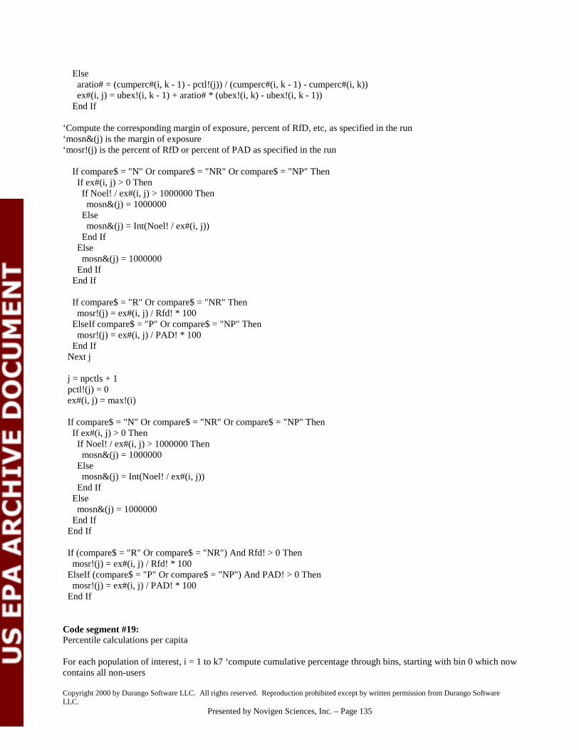
Copyright 2000 by Durango Software LLC. All rights reserved. Reproduction prohibited except by written permission from Durango SoftwareLLC.
Presented by Novigen Sciences, Inc. – Page 135
Else aratio# = (cumperc#(i, k - 1) - pctl!(j)) / (cumperc#(i, k - 1) - cumperc#(i, k)) ex#(i, j) = ubex!(i, k - 1) + aratio# * (ubex!(i, k) - ubex!(i, k - 1)) End If
‘Compute the corresponding margin of exposure, percent of RfD, etc, as specified in the run‘mosn&(j) is the margin of exposure‘mosr!(j) is the percent of RfD or percent of PAD as specified in the run
If compare$ = "N" Or compare$ = "NR" Or compare$ = "NP" Then If ex#(i, j) > 0 Then If Noel! / ex#(i, j) > 1000000 Then mosn&(j) = 1000000 Else mosn&(j) = Int(Noel! / ex#(i, j)) End If Else mosn&(j) = 1000000 End If End If
If compare$ = "R" Or compare$ = "NR" Then mosr!(j) = ex#(i, j) / Rfd! * 100 ElseIf compare$ = "P" Or compare$ = "NP" Then mosr!(j) = ex#(i, j) / PAD! * 100 End If Next j
j = npctls + 1 pctl!(j) = 0 ex#(i, j) = max!(i)
If compare$ = "N" Or compare$ = "NR" Or compare$ = "NP" Then If ex#(i, j) > 0 Then If Noel! / ex#(i, j) > 1000000 Then mosn&(j) = 1000000 Else mosn&(j) = Int(Noel! / ex#(i, j)) End If Else mosn&(j) = 1000000 End If End If
If (compare$ = "R" Or compare$ = "NR") And Rfd! > 0 Then mosr!(j) = ex#(i, j) / Rfd! * 100 ElseIf (compare$ = "P" Or compare$ = "NP") And PAD! > 0 Then mosr!(j) = ex#(i, j) / PAD! * 100 End If
Code segment #19:Percentile calculations per capita
For each population of interest, i = 1 to k7 ‘compute cumulative percentage through bins, starting with bin 0 which nowcontains all non-users

Copyright 2000 by Durango Software LLC. All rights reserved. Reproduction prohibited except by written permission from Durango SoftwareLLC.
Presented by Novigen Sciences, Inc. – Page 136
cumpercpc#(i, 0) = 100 - (bin#(i, 0) + (total1#(i) - total2#(i))) / total1#(i) * 100 'add all non-users to zero bin For j = 1 To nbins(i) cumpercpc#(i, j) = cumpercpc#(i, j - 1) - bin#(i, j) / total1#(i) * 100 If cumpercpc#(i, j) < 0 Then cumpercpc#(i, j) = 0 Next
k = 0 For j = 1 To npctls While cumpercpc#(i, k) > pctl!(j) And k < nbins(i) k = k + 1 Wend
If k = 0 Then aratio# = (100 - pctl!(j)) / (100 - cumpercpc#(i, k)) expc#(i, j) = aratio# * ubex!(i, k) Else aratio# = (cumpercpc#(i, k - 1) - pctl!(j)) / (cumpercpc#(i, k - 1) - cumpercpc#(i, k)) expc#(i, j) = ubex!(i, k - 1) + aratio# * (ubex!(i, k) - ubex!(i, k - 1)) End If Next
‘Compute the corresponding margin of exposure, percent of RfD, etc, as specified in the run‘mospcn&(j) is the margin of exposure‘mospcr!(j) is the percent of RfD or percent of PAD as specified in the run
ReDim mospcr!(npctls + 1), mospcn&(npctls + 1) If bw Then For j = 1 To npctls If compare$ = "N" Or compare$ = "NR" Or compare$ = "NP" Then If expc#(i, j) > 0 Then If Noel! / expc#(i, j) > 1000000 Then mospcn&(j) = 1000000 Else mospcn&(j) = Int(Noel! / expc#(i, j)) End If Else mospcn&(j) = 1000000 End If End If If (compare$ = "R" Or compare$ = "NR") And Rfd! > 0 Then mospcr!(j) = expc#(i, j) / Rfd! * 100 ElseIf (compare$ = "P" Or compare$ = "NP") And PAD! > 0 Then mospcr!(j) = expc#(i, j) / PAD! * 100 End If Next j mospcn&(npctls + 1) = mosn&(npctls + 1) mospcr!(npctls + 1) = mosr!(npctls + 1) End If
6. Subroutines used to compute distributions from distribution parameters
p! is always a random number >= 0 and <1.

Copyright 2000 by Durango Software LLC. All rights reserved. Reproduction prohibited except by written permission from Durango SoftwareLLC.
Presented by Novigen Sciences, Inc. – Page 137
Code segment #20:Sub lognormal (p!, m!, sd!, max!, c!)
m! is the meansd! is the standard deviationmax! is the highest value that the subroutine can returnc! is the residue amount returned
Dim mx!, sdx!
If m! > 0 Then mx! = Log((m! ^ 2) / ((m! ^ 2 + sd! ^ 2) ^ 0.5)) sdx! = (Log(1 + (sd! / m!) ^ 2)) ^ 0.5 Call normal(p!, mx!, sdx!, 0, c!) 'don't sent max to normal c! = Exp(c!) If c! < 0 Then c! = 0 If max! Then If c! > max! Then c! = max! End IfElse c! = 0End If
Code segment #21:Sub normal(p!, m!, sd!, max!, c!)m! is the meansd! is the standard deviationmax! is the highest value that the subroutine can returnc! is the residue amount returned
Dim Y!, top!, bottom!, quot! If p! = 0 Then p! = 0.0000001 If p! = 1 Then p! = 0.9999999 If p! <= 0.5 Then Y! = -Log(2 * p!) Else Y! = -Log(2 * (1 - p!)) End If If Y! <> 0 Then top! = 4 * Y! ^ 4 + 100 * Y! ^ 3 + 205 * Y! ^ 2 bottom! = 2 * Y! ^ 3 + 56 * Y! ^ 2 + 192 * Y! + 131 If bottom! Then quot! = top! / bottom! Else quot! = 0 End If c! = (quot! ^ 0.5) If p! <= 0.5 Then c! = -c! Else c! = 0 End If c! = c! * sd! + m! If max! Then If c! > max! Then c! = max! End If

Copyright 2000 by Durango Software LLC. All rights reserved. Reproduction prohibited except by written permission from Durango SoftwareLLC.
Presented by Novigen Sciences, Inc. – Page 138
End Sub
Code segment #22:Sub pareto(p!, a!, k!, max!, c!)
a! is the location variablek! is the shape variablemax! is the highest value that the subroutine can returnc! is the residue value returned
If p! < 1 Then c! = k! / (1 - p!) ^ (1/a!) If c! < 0 Then c! = 0 If max! Then If c! > max! Then c! = max! Else c! = 0 End If
Code segment #23:Sub triangular(p!, l!, m!, u!, c!)
l! is the low boundm! is the most likely valueu! is the high boundc! is the residue value returned
Dim h! If u! = l! Then c! = u! Else h! = (m! - l!) / (u! - l!) If p! <= h! Then c! = l! + (u! - l!) * (p! * h!) ^ 0.5 Else c! = l! + (u! - l!) * (1 - (1 - h! - p! + p! * h!) ^ 0.5) End If End If If c! < 0 Then c! = 0
Code segment #24:Sub uniform(p!, l!, u!, c!)
l! is the low boundu! is the high boundc! is the residue value returned c! = l! + p! * (u! - l!) If c! < 0 Then c! = 0
B. The Chronic Exposure Module
The Chronic module uses a data base of pre-calculated per-capita mean food consumption data (g/kg-bw-day) for eachfood (RAC) and food/foodform used in the CSFII surveys and residue data from a DEEM™ residue file to determine

Copyright 2000 by Durango Software LLC. All rights reserved. Reproduction prohibited except by written permission from Durango SoftwareLLC.
Presented by Novigen Sciences, Inc. – Page 139
the mean residue intake (in mg/kg-bw-day) for all individuals in the standard populations. The mean food consumptiondata base has been pre-calculated using the same algorithms used to generate the DEEM™ data base, except thatindividual food consumption amounts (after conversion from foods “as eaten” to constituent food-foodform amountsand summed by food-foodform type for the day) are rounded to the nearest 0.1 g in the DEEM™ Acute data base. Thepopulation-specific average daily food-foodform consumption amounts have not been rounded in the Chronic database, but instead saved in real number format (seven significant digits). In addition, food/foodform consumptionamounts for each individual were divided by the individual’s body weight before being summed into the accumulationvariables used to calculate the per-capita population-specific means. (The rationale for the rounding of individual foodconsumption records in the Acute program is discussed in the section addressing the Acute data base preparation.)
Mean per capita food consumption for estimating Chronic exposure can be calculated at either the food (RAC) orfood/foodform level, using residue data specified at either of the levels in the DEEM™ residue file. A DEEM™residue file can contain mixed residue data; that is, some foods can be specified at the food level and others at thefood/foodform level. The residues specified at the food level will be processed using daily food consumption data atthe food level; while any residues specified at the food/foodform level will be processed using daily food consumptiondata at the food/foodform level. (In the Acute module, all calculations are performed at the food/foodform level, evenif the residues are specified at the food level.)
Note that the same DEEM™ residue file can be used for both Acute and Chronic analysis. However, any residuedistribution functions and pointers in the residue file are ignored in the Chronic analysis; only the default residueamounts are used in a Chronic analysis. The residue file contains separate toxicology endpoints (NOEL and RfD) forchronic and acute analysis.
The Chronic analysis module calculates per capita daily mean, tmrc!(j), for each of the standard populations j = 1 to k4,by adding up exposure from each food in residue file and multiplying by the residue amount for that food, thenapplying adjusting factors and normalizing the exposure amounts to mg/kg-bw-day units. K4 = 27 when using theCSFII 1989-91 survey (which includes the Pacific zone) and k4 = 26 when using the CSFII 1994-96 survey. Thesemeans are reported directly, along with the margin of exposure estimates based on the chronic toxicology endpointsincluded in the residue file (or as modified when setting up the Chronic analysis).
1. Steps in a Chronic Analysis
Step 1: Read in the residue file specific to the analysis
(1) Read the toxicology endpoints(2) Read past the list of residue distribution functions (not used in Chronic)(3) Read the default residue amounts and conversion factors for each food/foodform in the residue file (ignore the
distribution pointers and ratios) as set up arrays as follows:
Tol!(i) = residue amount for ith Rac in residue file (i = 1 to totalfoods) Cf!(i) = conversion factor #1 for ith food Cf2!(i) = conversion factor #2 for ith food Rff(i) = number of food forms included in the residue file for this RAC FFTol!(l) = residue amount for food form FFF(l) FFCf!(l) = conversion factor #1 for food form FFF(l) FFCf2!(l) = conversion factor #2 for food form FFF(l)
Step 2. Read the NFB water consumption means for each standard population from supporting file. (See the list ofNFB water means above.) Meanw!(j) is per capita NFB water consumption from CSFII survey for each standardpopulation, as computed in DEEM™ Acute. RAC(435) is NFB water. Note that NFB water consumption is notreported for each drinking occasion, as are other foods, but rather reported as a total daily amount by the individual andincluded with the demographic records for that individiual.
Step 3. Open the two files of per capita food consumption means for the appropriate CSFII survey (1989-91 or 1994-96). (See the note on preparation of these means above.)

Copyright 2000 by Durango Software LLC. All rights reserved. Reproduction prohibited except by written permission from Durango SoftwareLLC.
Presented by Novigen Sciences, Inc. – Page 140
Mean!(j) is per-capita mean food consumption amounts (g/kg-bw-day) derived from the CSFII surveys for eachstandard population (j = 1 to k4), as retrieved from the Chronic food consumption data base.
K4 is the number of standard populations. (See the list of standard populations and their code above. Custompopulations cannot be used in the DEEM™ Chronic module. Note that the Pacific population group is not available inthe 94-96 survey because only four regions are available )Index(rac(i)) is the NSI index number for each of the 950 RACs (same as in the Acute module)The following variables are taken from the residue file used in the analysis:Nfx is number of RACs with residue amounts in the residue file.UseSecond is the Boolean operator used to determine if second adjustment factor is to be used.
Step 4. For each food or food/foodform in the residue file (all of which have a default residue amount), retrieve thefood consumption record for that food or food/foodform from the Chronic data base. Multiply the residue amount bythe food consumption amount for each of the k4 populations and sum for this exposure amount separately for eachpopulation. The resulting sums are reported as the total daily exposure for each population.
Step 5. Calculate the margin of exposure for each population using the toxicology endpoints and report.
See Code segement #26.
Step 6. If a critical commodity analysis and/or complete commodity analysis is desired, the same algorithms are usedas shown above, but consumption and residue amounts for individual foods/foodforms are reported as well as the sumor those amounts.
Code segment #25:Chronic module per capita daily exposure for each standard population
For i = 1 To nfx ‘For each food in residue file (1 to nfx) If index(rac(i)) Then If rff(i) = 0 Then If rac(i) = 435 Then For j = 1 To k4 mean!(j) = meanw!(survey, j) Next Else Get #1, index(rac(i)), mn94 For j = 1 To k4 mean!(j) = mn94.mean(j) ‘read in means for the k4 standard populations from data file Next j End If For j = 1 To k4 'these are not computed in display order tmrcx! = mean!(j) * tol!(i) * cf!(i) / 1000 If usesecond Then tmrcx! = tmrcx! * cf2!(i) tmrc!(j) = tmrc!(j) + tmrcx! Next j Else For l = kff(i) To kff(i) + rff(i) - 1 If rac(i) = 435 Then 'assumes that there is only one foodform for nfb water which is same as food For j = 1 To k4 mean!(j) = meanw!(survey, j) Next Else If nsiff(l) Then 'this is a valid ff Get #2, nsiff(l), mn94

Copyright 2000 by Durango Software LLC. All rights reserved. Reproduction prohibited except by written permission from Durango SoftwareLLC.
Presented by Novigen Sciences, Inc. – Page 141
ff = mn94.ff For j = 1 To k4 mean!(j) = mn94.mean(j) ‘read in means for the k4 standard populations from data file Next Else 'this ff is not available in fformxxn.fil, set means to 0 For j = 1 To k4 mean!(j) = 0 Next End If End If For j = 1 To k4 If mean!(j) Then tmrcx! = mean!(j) * fftol!(l) * ffcf!(l) / 1000 If usesecond Then tmrcx! = tmrcx! * ffcf2!(l) tmrc!(j) = tmrc!(j) + tmrcx! End If Next j Next l End If End If Next i
Code segment #26:Computation of percent of RfD or percent of PAD
rfdchonic! = RfD or PAD to be used in the analysisprfd! = percent RfD or % PAD as outputmeanindex(survey, j) is used to reorder the order in which the k4 populations are reportednoelchronic! = chronic NOEL measurepnoelfx! = exposure as percent of Noelmos! = margin of exposureqstar! = Q starq! = lifetime risk
If compare$ = "R" Or compare$ = "P" Then For j = 1 To k4 'display order now o = meanindex(survey, j) 'the corresponding mean and pop$() location If tmrc!(o) Then prfd! = tmrc!(o) * 100 / rfdchronic! End If Next jElseIf compare$ = "N" Then 'noel For j = 1 To k4 o = meanindex(survey, j) 'the order we want to display them pnoelfx! = tmrc!(o) * 100 / noelchronic! If tmrc!(o) Then mos! = noelchronic! / tmrc!(o) Else mos! = 0 NextElse For j = 1 To k4 o = meanindex(survey, j) 'the order we want to display them If tmrc!(o) Then q! = tmrc!(o) * qstar! End If NextEnd If

Copyright 2000 by Durango Software LLC. All rights reserved. Reproduction prohibited except by written permission from Durango SoftwareLLC.
Presented by Novigen Sciences, Inc. – Page 142
2. Non-Food-Based (NFB) Water consumption means (mg/kg-bw-day) by population (calculated in the acutemodule, used in Chronic module) (See population definitions corresponding to indices below.)
CSFII 89-91: meanw!(1) = 14.09 meanw!(2) = 14.26 meanw!(3) = 14.98 meanw!(4) = 13.66 meanw!(5) = 13.48 meanw!(6) = 12.47 meanw!(7) = 13.99 meanw!(8) = 14.07 meanw!(9) = 14.86 meanw!(10) = 16.77 meanw!(11) = 13.4 meanw!(12) = 16.35 meanw!(13) = 15.19 meanw!(14) = 25.41 meanw!(15) = 9.45 meanw!(16) = 28.28 meanw!(17) = 25.66 meanw!(18) = 17.06 meanw!(19) = 14.54 meanw!(20) = 18.57 meanw!(21) = 11.39 meanw!(22) = 13.24 meanw!(23) = 12.79 meanw!(24) = 12.14 meanw!(25) = 10.98 meanw!(26) = 12.98 meanw!(27) = 14.86CSFII 94-96: meanw!(1) = 13.077 meanw!(2) = 13.433 meanw!(3) = 13.607 meanw!(4) = 12.562 meanw!(5) = 12.68 meanw!(6) = 11.308 meanw!(7) = 13.471 meanw!(8) = 12.487 meanw!(9) = 15.201 meanw!(10) = 15.799 meanw!(11) = 12.704 meanw!(12) = 13.836 meanw!(13) = 14.128 meanw!(14) = 12.674 meanw!(15) = 6.29 meanw!(16) = 14.965 meanw!(17) = 19.039 meanw!(18) = 13.353 meanw!(19) = 14.442 meanw!(20) = 21.098 meanw!(21) = 10.645 meanw!(22) = 12.239

Copyright 2000 by Durango Software LLC. All rights reserved. Reproduction prohibited except by written permission from Durango SoftwareLLC.
Presented by Novigen Sciences, Inc. – Page 143
meanw!(23) = 12.237 meanw!(24) = 10.848 meanw!(25) = 12.809 meanw!(26) = 11.7
3. Subroutine to calculate body weight for CSFII participants who do not have a recorded bodyweight
Infant weights are computed by age in month (0-11) and by sex (1 = male, 2 = female)All others are computed by age in years (0-90) and by sex (1 = male, 2 = female); body weights for participants above90 are assumed to be the same as for age 90. These body weights were derived from those individuals in the sameCSFII survey for which body weight is provided (1989-91 or 1994-96), using average body weight within age intervalsin which weight does not vary significantly by age, and using simple straight-line curve fitting techniques for intervalsin which a straight line characterizes the weight distribution.
Note that these body weights were computed for individuals without body weights at the time that the acute andchronic data bases were developed for use with DEEM™. Body weight computations are not made during the acute orchronic analyses.
(1) Subroutine compbw for 1994-96 CSFII survey participants
Sub compbw(infwt(), agewt())
Dim mFor m = 0 To 11 infwt(1, m) = 10 + 1.24 * m infwt(2, m) = 9 + 1.3 * mNextDim yFor y = 1 To 5 agewt(1, y) = 22.1 + 4.7 * y agewt(2, y) = 19.7 + 4.7 * yNextFor y = 6 To 11 agewt(1, y) = -1 + 8.5 * y agewt(2, y) = -3.4 + 8.66 * yNextFor y = 12 To 16 agewt(1, y) = -51 + 13.6 * y agewt(2, y) = 6.6 + 8.4 * yNextFor y = 16 To 18 agewt(1, y) = 160 agewt(2, y) = 132NextFor y = 19 To 21 agewt(1, y) = 171 agewt(2, y) = 137NextFor y = 22 To 25 agewt(1, y) = 176 agewt(2, y) = 143NextFor y = 26 To 30 agewt(1, y) = 184 agewt(2, y) = 146

Copyright 2000 by Durango Software LLC. All rights reserved. Reproduction prohibited except by written permission from Durango SoftwareLLC.
Presented by Novigen Sciences, Inc. – Page 144
NextFor y = 31 To 40 agewt(1, y) = 184 agewt(2, y) = 150NextFor y = 41 To 50 agewt(1, y) = 190 agewt(2, y) = 155NextFor y = 51 To 60 agewt(1, y) = 187 agewt(2, y) = 161NextFor y = 61 To 70 agewt(1, y) = 182 agewt(2, y) = 154NextFor y = 71 To 80 agewt(1, y) = 175 agewt(2, y) = 147NextFor y = 81 To 90 agewt(1, y) = 161 agewt(2, y) = 131Next
End Sub
(2) Subroutine compbw for 1989-91 CSFII survey participants
Sub compbw(infwt(), agewt())Dim m, yFor m = 0 To 11 infwt(1, m) = 10 + 1.3 * m infwt(2, m) = 9 + 1.3 * mNextFor y = 1 To 5 agewt(1, y) = 21 + 4.8 * y agewt(2, y) = 21 + 4.8 * yNextFor y = 6 To 11 agewt(1, y) = -4 + 9.36 * y agewt(2, y) = -4 + 9.36 * yNextFor y = 12 To 15 agewt(1, y) = -4 + 9.36 * y agewt(2, y) = 30 + 6.44 * yNextFor y = 16 To 18 agewt(1, y) = 155 agewt(2, y) = 130NextFor y = 19 To 21 agewt(1, y) = 165 agewt(2, y) = 134

Copyright 2000 by Durango Software LLC. All rights reserved. Reproduction prohibited except by written permission from Durango SoftwareLLC.
Presented by Novigen Sciences, Inc. – Page 145
NextFor y = 22 To 25 agewt(1, y) = 171 agewt(2, y) = 138NextFor y = 26 To 30 agewt(1, y) = 177 agewt(2, y) = 139NextFor y = 31 To 40 agewt(1, y) = 181 agewt(2, y) = 146NextFor y = 41 To 50 agewt(1, y) = 187 agewt(2, y) = 151NextFor y = 51 To 60 agewt(1, y) = 180 agewt(2, y) = 157NextFor y = 61 To 70 agewt(1, y) = 179 agewt(2, y) = 151NextFor y = 71 To 80 agewt(1, y) = 174 agewt(2, y) = 144NextFor y = 81 To 90 agewt(1, y) = 155 agewt(2, y) = 129NextFor y = 91 To 100 agewt(1, y) = 144 agewt(2, y) = 130Next
End Sub
C. The RDFgen™ Module
RDFgen™ uses QA’ed sets of spreadsheets containing up-to-date monitoring data from the most widely used source,the Pesticide Data Program (PDP) of the U.S. Department of Agriculture (USDA). These sets of spreadsheets areready for immediate use with RDFgen™, and are referred to by the following titles: “RDFgen™ pre-extracted PDPdata set formatted for RDFgen™ Individual Analyte Mode” and “RDFgen™ pre-extracted PDP data set formatted forRDFgen™ Cumulative Mode.”

Copyright 2000 by Durango Software LLC. All rights reserved. Reproduction prohibited except by written permission from Durango SoftwareLLC.
Presented by Novigen Sciences, Inc. – Page 146
Additionally, to allow creation of RDFgen™ Cumulative Mode or Individual Analyte Mode PDP residue inputspreadsheets filtered for specific sample attributes (such as origin or date collected), Novigen maintains a pre-extracteddata set integrating all PDP sample database and residue database information, plus the following helpful standardizedfields:
" COMMOD_NAM (Translated version of the two-character COMMOD field, including separation ofprocessed commodities that share COMMOD code with unprocessed commodities, such as greenbeans/processed green beans and peaches/canned peaches).
" FULL_PESTN (Standardized version of two-character PEST_NAME field)." BOOKYEAR (PDP data annual report year to which the record belongs)." YEARY2K (Ensures continued ability to correctly sort and query based on sample date)." DETECT (Y/N field indicating whether sample is a detect or non-detect sample)." ORIGINSTD (Standardized version of ORIGIN field, facilitating separation of domestic samples, imported
samples, and samples of unknown origin).
This series of spreadsheets is referred to as the RDFgen™ full Pre-extracted PDP data set. Creation of RDFgen™Cumulative or Individual Analyte Mode PDP residue input spreadsheets or user-defined subsets of the RDFgen™ fullPre-extracted PDP data set is automated by the RDFgen™ Input Generator™ Excel add-in.
RDFgen™ can operate in two primary modes: Individual Analyte Mode and Cumulative Mode. The IndividualAnalyte mode allows the user to perform the following residue adjustments on any single analyte residue distribution:
" Percent Crop Treated" Decompositing
The Cumulative mode allows the user to perform the following residue adjustments on any combination of compounds,provided those individual samples have been tested for co-incident residues:
" Percent Crop Treated" Estimation of concentrations in individual fruits/vegetables based on values in a composite sample (referred to
through this document as “decompositing”)" Relative Potency" Processing Factors
RDFgen™ may be launched from within DEEM™ or used independently.
The RDFgen™ module of DEEM™ accepts as input any residue data spreadsheet that has been formatted according toa specified format. The user is responsible for the quality and representativeness of the data contained in userdeveloped or modified spreadsheets. In general, Individual Analyte Mode input spreadsheets contain distributions forvarious commodities tested for a particular chemical, while Cumulative Mode input spreadsheets generally containdistributions for various chemicals tested on a particular commodity. Cumulative Mode should be used when it isdesired to combine residue data from multiple analytes into a single distribution. Note that RDFgen™ CumulativeMode will only use samples from the Cumulative Mode input spreadsheets that have been tested for all of the analytesthat are selected for inclusion. Individual analyte mode should be employed when residue distribution adjustments aregoing to be performed on single analyte’s residue data.


