The Economic Value of Fundamental and TechnicalInformation in Emerging Currency Markets∗
Gerben de Zwart†
ING Investment Management andRSM Erasmus University
Thijs MarkwatEconometric Institute and
Erasmus Research Institute of Management
Laurens SwinkelsRobeco Quantitative Strategies and
Erasmus Research Institute of Management
Dick van DijkEconometric Institute
Erasmus University Rotterdam
January 2008
Abstract
We measure the economic value of information derived from macroeconomicvariables and from technical trading rules for emerging markets currency in-vestments. Using a sample of 23 emerging markets with a floating exchangerate regime over the period 1995-2007, we document that both types of in-formation can be exploited to implement profitable trading strategies. In linewith evidence from surveys of foreign exchange professionals concerning theuse of fundamental and technical analysis, we find that combining the twotypes of information improves the risk-adjusted performance of the invest-ment strategies.
Keywords: Emerging markets, Foreign exchange rates, Structural exchangerate models, Technical trading, Heterogeneous agentsJEL Classification: C53, F31, G15
∗We are grateful to Kees Bouwman, Ron Jongen and Marno Verbeek for helpful suggestions.We would also like to thank participants of the Conference on Heterogeneous Agents in FinancialMarkets at the Radboud University Nijmegen, the Nonlinear Economics and Finance ResearchCommunity at Keele University, and seminar participants at the University of Groningen. We aregrateful to Robeco for providing the data.
†Corresponding Author: ING Investment Management, P.O. Box 90470, NL-2509 LLDen Haag, The Netherlands. E-mail addresses are [email protected], [email protected],[email protected], and [email protected]

The Economic Value of Fundamental and TechnicalInformation in Emerging Currency Markets
December 2007
Abstract
We measure the economic value of information derived from macroeconomicvariables and from technical trading rules for emerging markets currency in-vestments. Using a sample of 23 emerging markets with a floating exchangerate regime over the period 1995-2007, we document that both types of in-formation can be exploited to implement profitable trading strategies. In linewith evidence from surveys of foreign exchange professionals concerning theuse of fundamental and technical analysis, we find that combining the twotypes of information improves the risk-adjusted performance of the invest-ment strategies.
Keywords: Emerging markets, Foreign exchange rates, Structural exchangerate models, Technical trading, Heterogeneous agentsJEL Classification: C53, F31, G15

1 Introduction
The literature on exchange rate forecasting has extensively analyzed the predictive
content of two types of information: news on macroeconomic fundamentals as used
in structural exchange rate models, and information from historical prices as used
in technical trading rules. Meese and Rogoff’s (1983) finding that structural models
cannot outperform a naive random walk forecast at short horizons still stands after
25 years of intense research, see Cheung et al. (2005) for a recent assessment. There is
somewhat more supportive evidence for the usefulness of macroeconomic information
for forecasting exchange rates at longer horizons, see Mark (1995), Kilian (2001)
and Berkowitz and Giorgianni (2001), among others. In general, the performance of
technical trading rules at short horizons has been found to be considerably better,
see Sweeney (1986), Levich and Thomas (1993) and Neely and Weller (1999), with
Menkhoff and Taylor (2007) providing a recent comprehensive survey. Nevertheless,
Olson (2004), Pukthuanthong-Le et al. (2007) and Neely et al. (in press) report that
the profitability of technical trading rules has weakened substantially in recent years,
at least for developed currencies.
The predictive ability of structural exchange rate models and technical trading
rules has generally been considered in isolation. This is quite remarkable, in the
sense that surveys among foreign exchange market participants invariably indicate
that they regard both types of information to be important factors for determining
future exchange rate movements, see Taylor and Allen (1992), Menkhoff (1997),
Lui and Mole (1998), Cheung and Chinn (2001), and Gehrig and Menkhoff (2004).
Not surprisingly then, most foreign exchange professionals use some combination of
fundamental analysis and technical analysis for their own decision making, with the
relative weight given to technical analysis becoming smaller as the forecasting (or
trading) horizon becomes longer.
The weights assigned to fundamental and technical information for a given hori-
zon may also vary over time. For example, Frankel and Froot (1990) provide em-
pirical evidence for the switch of many professional forecasters from being “fun-
damentalists” (using structural models and macro data) to acting as “chartists”
(using technical trading rules) during the second half of the 1980s. They motivate
this changing behavior by the fact that fundamentalists experienced large negative
1

returns in the mid-1980s, when currency prices deviated from their fundamental
values. The concept of switching behavior has been formalized in so-called het-
erogeneous agents models. Brock and Hommes (1997, 1998) develop equilibrium
models in which agents update their beliefs about the profitability of investment
strategies based on their past performance. These models show that rational in-
vestors can switch between simple (costless) strategies and sophisticated (costly)
strategies. When all investors follow the simple strategy prices may diverge from
their fundamental value, making it worthwhile for investors to engage in sophisti-
cated strategies, because expected profits increase. Prices are then pushed back to
their fundamental value and the expected net profits for sophisticated investors are
negative, which leads them to switch back to simple and costless strategies that
might again result in prices moving away from their fundamental value. These het-
erogeneous agents models have recently been applied to currency markets, explicitly
allowing for the presence of both chartists and fundamentalists, see Chiarella et al.
(2006), and De Grauwe and Grimaldi (2005, 2006). The relative importance of these
two types of traders (and, hence, the two types of information) varies over time as
investors are assumed to switch between strategies according to their relative past
performance. De Grauwe and Markiewicz (2006) offer an alternative interpretation
of these models, in which market participants combine technical analysis and funda-
mental information in order to forecast future foreign exchange rates, with weights
varying over time as a function of past profitability.
Most research on exchange rate forecasting has focused on developed markets.
Scarcely any attention has been paid to emerging market currencies, possibly due to
the fact that many emerging countries maintained a fixed or pegged exchange rate
regime until fairly recently.1 Since the mid-1990s, approximately, more and more
countries have switched to a floating exchange rate regime, such that by now the
time series length as well as the cross-sectional breadth are sufficient to warrant a
meaningful investigation of exchange rate predictability in emerging markets. To the
best of our knowledge we are the first to conduct such an analysis. Previous empirical
research on heterogeneous agents models has also been limited to developed currency
1One aspect of exchange rate forecasting in emerging markets that did receive ample attention inthe past is prediction of currency crises, in particular by means of so-called early warning systems,see Kaminsky (2006) for a detailed overview.
2

markets, such as Vigfusson (1997) and De Jong et al. (2006), which report only
limited evidence supporting the switching behavior that is assumed in the theoretical
models. Our study contributes to this literature by examining the profitability of
trading strategies that switch between fundamentalist and chartist strategies based
on past performance in emerging currency markets.
In this paper we conduct a comprehensive analysis of the economic value of tech-
nical and fundamental information in emerging currency markets. Specifically, we
assess the performance of currency trading strategies based on monthly fundamen-
tal information derived from the real interest rate differential, GDP growth, and the
ratio of money supply to foreign exchange reserves, as well as a set of daily moving
average technical trading rules. We implement these strategies for all freely float-
ing emerging market currencies relative to the US dollar over the period 1995-2007.
We also consider combined strategies in which both chartist and fundamentalist
information are used, in line with the actual behavior of market participants, as
discussed above. In particular, we examine a dynamic combination scheme with
time-varying weights according to the relative profitability of the fundamental and
technical strategies. As a benchmark we employ a naive strategy that assigns con-
stant and equal weights to the two types of information. Throughout the empirical
analysis, we also consider nine developed currencies as a control sample.
Our results can be summarized as follows. First, both fundamentalist and
chartist strategies generate economically and statistically significant Sharpe ratios
for emerging currency markets. This finding is consistent with McNown and Wallace
(1989), who document that fundamentalist trading strategies perform well in four
emerging markets over the period 1972-1986. Our positive results for technical trad-
ing rules provide out-of-sample evidence for the profits described by Martin (2001)
and Lee et al. (2001a) for the early 1990s.
Second, we document that naively combining chartist and fundamentalist strate-
gies generates positive risk-adjusted returns that are both economically and sta-
tistically significant. Moreover, the performance of the combined strategy is much
more consistent and stable across currencies than the individual fundamentalist and
chartist strategies. This provides convincing evidence for the complementary value
of technical and fundamental information as suggested by questionnaires among
currency traders. The dynamic combined strategies, where the weights assigned to
3
fundamentalist and chartist strategies vary according to their past performance, do
not increase the profitability of the trading strategy relative to the naive combina-
tion. Thus, we find only limited empirical support for the enhanced profitability
of the investment strategies based on the heterogeneous agents models of Chiarella
et al. (2006) and De Grauwe and Grimaldi (2005, 2006).
Third, for developed currency markets we find that fundamental trading strate-
gies render statistically and economically significant Sharpe ratios, but this is not
the case for the chartist strategies. This result is in line with Abhyankar et al.
(2005), who conclude that investors may benefit from fundamental exchange rate
models trading the US dollar against the Canadian dollar, Japanese Yen, and British
Pound over the period 1977-2000. It also corroborates the findings of Olson (2004),
Pukthuanthong-Le et al. (2007) and Neely et al. (in press), who document that
returns to technical trading strategies in developed markets have declined over time.
The remainder of this paper is organized as follows. In Section 2 we describe
the data. We examine the performance of the fundamentalist and chartist strategies
individually in Sections 3 and 4, respectively. In Section 5 we integrate the chartist
and fundamentalist information into combined strategies. Finally, we conclude in
Section 6.
2 Data description
Our analysis is most relevant for exchange rates under a free float, as currency
prices in this system are determined in principle by demand and supply, although
intervention activities of central banks cannot be ruled out completely.2 Data before
1995 is thus not considered, as most of the countries in our sample adopted a floating
exchange rate regime around that time or later.3 In total we examine the currencies
2We refer to the conference notes of the IMF ‘High-Level seminar on exchange rate regimes:Hard peg or free floating?’ for an overview of central bank intervention activity in the emergingcurrency markets, see http://www.imf.org/external/pubs/ft/seminar/2001/err/eng/.
3In the late 1980s many emerging market countries pegged their currency to the US dollaror a basket of developed currencies to achieve price stability after a period of (hyper-)inflation.Some countries used a crawling peg, where the currency was allowed to depreciate at a steadyrate such that the local inflation rate could be higher than the pegged rate. A side effect of theemerging markets currency crises during the 1990s has been that most emerging markets changedtheir exchange rate system from a pegged to a floating regime. Currently, only a small numberof emerging market countries still maintain a (crawling) peg regime: China (pegged to the USdollar), Russia (pegged to a basket of the US dollar and euro), Vietnam (US dollar) and Pakistan
4
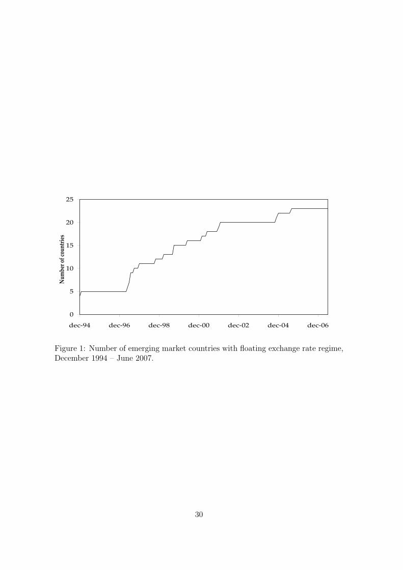
of 23 emerging markets which currently have a (managed) floating exchange rate
system: the Argentine peso, Brazilian real, Chilean peso, Colombian peso, Mexican
peso and Peruvian sol from Latin-America; the Indian rupee, Indonesian rupiah,
Kazakhstan tenge, Korean won, Malaysian ringitt, Phillipine peso, Sri Lanka rupee,
Taiwanese dollar and Thai bath from Asia; and the Czech koruna, Hungarian forint,
Israeli shekel, Polish zloty, Romanian leu, Slovak koruna, South African rand, and
Turkish lira from Europe, Middle-East, and Africa (EMEA). All of these currencies
became floating at some point between January 1995 and June 2007. Figure 1
shows the historical development of the number of emerging market countries with a
floating exchange rate regime in our sample. The exact dates of the the currencies’
floats are given in Table 1.
- insert Figure 1 about here -
We employ daily and monthly exchange rates for the technical trading rules and
the fundamental models, respectively. The exchange rates correspond to Reuters
07:00 GMT middle rate fixings against the US dollar.4 All exchange rates are ex-
pressed in the standard way, that is, as the price of one US dollar in the emerging
market currency. The sample period runs from January 1, 1995 to June 30, 2007
(3260 daily and 150 monthly observations), where it is to be understood that each
currency is included in the analysis only six months after the start of its floating
exchange rate regime. In practice, most investors will hold off investing in a currency
for some time to avoid the often dramatic exchange rate movements immediately
following the float of a currency. The market has sufficiently ‘cooled down’ after
about half a year for most currencies.
A common instrument that can be used for sec investments in the currency
market is the currency forward contract. These instruments enable us to invest in
a currency without owning any underlying assets, for example bonds or stocks, in
the country. With the help of the forward contract we lock in a specific foreign
exchange rate in the future. The investment return on a currency is then defined as
(US dollar).4Results for the Eastern European currencies (CZK, SKK, PLN, HUF and RON) relative to
the EUR are similar and available upon request.
5
the difference between this forward rate and the future spot rate:
rt = st − ft−1,t (1)
where st is the log spot rate at time t and ft−1,t is the log forward rate at time t− 1
maturing at time t. In the absence of arbitrage opportunities, the forward rate is
given by:
Ft−1,t = St−1 exp(iEMt−1 − iUS
t−1) (2)
where iEMt−1 and iUS
t−1 are the cash interest rates in the emerging country and the US,
respectively. The cash rate is generally the offshore deposit rate for money deposited
in the currency and maturity that matches the maturity of the forward contract, for
example the London Interbank Offered Rate (LIBOR) for US dollars.5 Substitution
of (2) in (1) leads to the return on a foreign exchange investment:
rt = st − st−1 + iUSt−1 − iEM
t−1 (3)
Many studies on trading strategies for developed exchange rate markets disregard
the interest rate differential as the influence on profitability is found to be negligible,
see Sweeney (1986) and LeBaron (1999), among others. For emerging markets the
interest rate differentials can be substantial, as shown below, and therefore should
be taken into account for a fair judgement of the investment returns. We obtain
interest rates from two different sources: Bloomberg and the IMF International
Financial Statistics (IFS) database. The monthly IFS data has the advantage that it
is available for a longer time period, while the Bloomberg data is updated on a daily
basis. As daily data entails more information, Bloomberg three-month interbank
interest rates are used from the moment they are available; otherwise IFS three-
month deposit rates are used.6
- insert Table 1 about here -
5The cash rates are quoted on an annualized basis. For our return calculations the cash ratesare scaled to the a daily or monthly basis by dividing the rate by 360 days and multiplying by thenumber of days that a position will be held.
6We use the three-month deposit rates because our final trading strategy (see Section 5) holdsits positions for three months on average.
6

Summary statistics for the monthly returns of the emerging markets currencies
are reported in Table 1.7 The Turkish lira has the best performance with an annu-
alized mean return of 25.6 percent per year, relative to the US dollar. Note that the
Turkish lira hardly moved during its floating period (February 2001 - June 2007),
but an investor was more than compensated by the interest rate differential of 25.4
percent per year. The Taiwanese dollar has the worst performance with an average
return of –2.45 percent per year. The annualized standard deviations of the monthly
returns range between a low of 3.4 percent for the Malaysian ringitt (July 2005 -
June 2007) and a high of 26.5 percent for the Indonesian Rupiah (August 1997 - June
2007). For 12 of the 23 currencies the kurtosis is (much) higher than three, indicat-
ing a high peak and fat tails in the empirical distribution of the returns relative to
a normal distribution. The tail behavior of emerging market currencies is studied in
detail by Candelon and Straetmans (2006). The unreported Jarque-Bera test shows
that almost none of the currency returns are Gaussian, due to the high kurtosis and
the nonzero skewness. The example of the Turkish lira mentioned above already
suggests that we should not disregard the interest rate differential when computing
the investment return on the emerging market currencies. This is confirmed by the
last two columns of Table 1, showing that the average interest rate differential is
even larger than the spot rate return for 11 out of 23 currencies.
Table 1 also includes summary statistics of our developed markets control sam-
ple. This sample holds the G10 currencies: Australian dollar, Canadian dollar, UK
pound, Japanese yen, Euro, Swiss franc, Norwegian krone, Swedish krona, and the
New Zealand dollar, all relative to the US dollar. We use the German Deutschmark
for the history of the euro prior to 1999. The New Zealand dollar performs best
with an annualized return of 3.7 percent. The Japanese yen shows the worst perfor-
mance with an average return of −7.1 percent per year. The average volatility is 9.4
percent, with much less variation across currencies than for the emerging markets.
Finally, we compute the cross-correlations of the monthly returns. The average
correlation between all possible pairs of emerging markets exchange rates is 0.18.
Most correlations are in fact close to zero, although some currencies within the
7The (unreported) descriptive statistics for the daily returns show similar patterns, althoughthe kurtosis is higher. This corresponds quite well with the stylized fact of asset returns that non-normality (in particular peakedness and fat tails) becomes more pronounced at higher frequencies
7
same region have a correlation of up to 0.50 for Asia and 0.75 for Europe. These
small correlations are advantageous for our empirical analysis, as it means that the
trading strategies can benefit from diversification if we combine the currencies in a
portfolio. The cross-correlations among emerging market currencies are considerably
smaller than those for the developed exchange rates, which generally exceed 0.75.
For example, the correlation between the euro and Swiss Franc is equal to 0.94.
The main exception is the correlation of the Japanese yen with the other developed
currencies, which is substantially lower and equals 0.32 on average.
3 Fundamentalist trading strategies
Fundamentalists believe that the exchange rate is intimately linked to macroeco-
nomic variables such as output, inflation, and the trade balance, among others.
Hence, news in these economic “fundamentals” is responsible for exchange rate move-
ments. A wide variety of structural exchange rate models is available that might be
used for forecasting the future exchange rate. Cheung et al. (2005) conclude that
“old-fashioned”, basic structural models, such as the real interest rate differential
(see Frankel (1979), for example) perform at least as good as more recent, elaborate
models. This motivates us to use relatively simple structural models in our empirical
analysis. In particular, we assume that fundamentalists derive their exchange rate
forecasts from information on the real interest rate differential, the growth rate of
GDP, and the growth rate of the ratio of the money supply (M2) to foreign exchange
reserves.8 Furthermore, we do not explicitly estimate regression models that include
these variables as regressors, but instead we simply use them to generate buy and sell
signals for the different currencies based on a prediction of the sign of the exchange
rate return in the next month, as explained in detail below. On the one hand, this
is motivated by the fact that the time period during which the emerging market
currencies are floating generally is already rather short. Using part of the available
sample for model estimation would leave only a very limited number of observations
for out-of-sample forecasting. On the other hand, as pointed out by Leitch and Tan-
ner (1991), among others, correctly forecasting the sign of asset returns is perhaps
8Data on inflation, GDP, M2 and Reserves are taken from the IFS database. The Taiwan datacomes from the website of the Taiwanese Central Bank.
8

more crucial than forecasting their magnitude when it comes to economic forecast
evaluation measures such as the performance of trading strategies.
The three macroeconomic variables are used to generate buy and sell signals as
follows. First, we consider the real interest rate differential (RID) as an example.
Given the high inflation in emerging markets we do not consider the nominal dif-
ferential but the real interest differential, see Isaac and de Mel (2001) for discussion
of the real interest rates differential literature. The RID forecasting rule can be
thought of in terms of the variable RID t, defined as
RID t =
1 if iEM
t−1 − πEMt−1 < iUS
t−1 − πUSt−1,
−1 otherwise,(4)
where iXt−1 is the short-term interest in country X and πXt−1 is the corresponding
inflation rate. The values 1 and −1 for RID t correspond to a long position in the US
dollar and in the emerging market currency, respectively. In other words, in month
t we take a long (short) position in the emerging market currency if its real interest
rate in month t− 1 is above (below) the US one.
The levels of GDP in the countries under consideration differ substantially, there-
fore we consider the relative GDP growth rates as more appropriate for forecasting
the direction of the future exchange rate movement. As higher GDP growth leads to
higher income, we expect an increased demand for money and therefore a stronger
currency. Hence, we take a long position in the emerging market currency if its GDP
growth over the past 12 months was higher than the US GDP growth, and a short
position when GDP growth was lower. The GDP buy-sell indicator may thus be
defined as
GDP t =
1 if ∆GDPEM
t−1 < ∆GDPUSt−1,
−1 otherwise,(5)
where ∆GDPXt−1 is the GDP growth rate in country X.
Our third and final fundamental variable, the growth rate of the ratio of M2
money supply (M2) to foreign exchange reserves (RES), influences exchange rates
through the rules of demand and supply. A loss of international reserves or a large
rise in the domestic money supply can lead to less confidence in a currency and
therefore less demand and more supply. Let ∆(
M2Xt−1
RESXt−1
)denote the 12-month growth
rate of the money-reserves ratio in country X in period t−1. The investment decision
9
is based on the buy-sell indicator
M 2Rt =
1 if ∆
(M2EM
t−1
RESEMt−1
)> ∆
(M2US
t−1
RESUSt−1
)
−1 otherwise,(6)
that is, we take a long position in the currency with the lowest growth of the money-
reserves ratio.
Although in the following we also consider the strategies based on the RID,
GDP and M 2R signals individually, we mainly focus on an investor who combines
the different fundamental signals for making her ultimate decision. Of course, there
are infinitely many ways to combine the three pieces of information. Here we take
the simple average of the three signals, that is
Ft =RID t + GDP t + M 2Rt
3. (7)
Note that the combined fundamentalist signal will be +1 if all three strategies are
negative on the non-US currency, and vice versa.
The fundamental buy-sell indicators RID t, GDP t, M 2Rt, and Ft are used to im-
plement trading strategies with monthly rebalancing. The return of the fundamental
strategy based on signal Yt for currency i, rYi,t, is computed as rY
i,t = Yt ·rt,i, where ri,t
is the return on a short position in the non-US currency (and thus a long position
in the US dollar) for month t. This is a long-short investment strategy, because we
will be long in one currency and short in the other currency. The risk free rate is
therefore an appropriate benchmark. For this reason we use the Sharpe Ratio as the
main criterion to judge the performance of the strategies, because our returns are
self financed (excess) returns.
The strategies are implemented for all the emerging and developed currencies
individually. In addition, we consider the performance of equally-weighted (EW)
and volatility-weighted (VW) portfolios. The weights in the latter portfolio are set
proportional to the inverse of the ex post volatility of the spot rates, as measured by
the standard deviation over the whole sample period. This is based on the idea that
in that case each currency contributes an approximately equal amount to the total
portfolio risk. The return of the equal-weighted and volatility weighted portfolios
are computed as
rY,EWt =
1
nt
∑iεΩt
rYi,t and rY,V W
t =1∑
iεΩt
1σi
∑iεΩt
1
σi
rYi,t (8)
10
where Ωt is the set of available currencies at time t, nt the number of currencies
in Ωt at t, and σi is the volatility of the spot rate for country i. We acknowledge
that the use of the full-sample standard deviation to weight the currencies entails
some form of data-snooping and also avoids the fact that, especially for the emerging
markets, the volatilities vary over time. More advanced weighting schemes using an
ex ante volatility measure would, however, put serious limitations on the sample
period available for forecast evaluation. Hence, these are left for future research.
- insert Table 2 about here -
The results for the fundamental strategies based on the individual RID, GDP
and M 2R signals are summarized in Table 2. Several interesting conclusions emerge.
First, the performance of the strategies for individual currencies based on RID or
GDP is on average positive, while the performance of the M 2R strategy is mostly
negative. Especially for the GDP strategy the average return is also significantly
different from zero (in terms of t-values at a 5 percent significance level) for quite
a large number of currencies, while no significantly negative average returns occur.
The M 2R strategy renders a significantly negative average return for two individual
countries, compared to only one significantly positive return. Thus, the RID and
GDP strategies seem to provide considerably more accurate forecasts of future ex-
change rate movements than the M 2R strategy. Within the strategies the results
vary dramatically across countries. For example, the average returns on the RID
strategy range between 14.3 and –5.1 percent for Turkey and Kazakhstan, respec-
tively. For the other strategies the variation is even more pronounced. This also
shows up in the volatilities of the individual strategies, see India and Slovakia, for
example.
For the developed currencies, we also find that the M 2R strategy performs rela-
tively worse for most countries. A difference with the emerging markets is, however,
that the real interest rate differential seems to be more informative for the exchange
rate movements than the relative GDP growth rates. Except for the Swedish krona,
the RID strategy results in positive average returns for all developed currencies,
which furthermore are statistically significant for four of the eight countries.
The results in Table 2 do not take into account transaction costs. To investigate
the influence of such costs, we record the number of transactions in each strategy
11

and compute break-even transaction costs. The average number of transactions per
year is equal to approximately 1, 0.5 and 1.5 for the RID, GDP and M 2R strategies,
respectively. Compared to trend strategies these numbers are rather low (as shown in
the next section), which also results in relatively high levels of break-even transaction
costs. For most countries and strategies having a positive performance, break-even
transaction costs exceed 2 percent, which for most currencies is clearly above the
level of transactions costs encountered in practice by a large institutional investor.
More detailed results on the RID, GDP and M 2R strategies are not shown here to
save space, but are available upon request.
Combining the individual currencies in a portfolio results in significantly posi-
tive returns for the RID- and GDP -based strategies, except for the equally-weighted
emerging market portfolio based on the real interest rate differential. The benefits
of diversification across currencies become clear by noting the low volatilities of the
portfolio returns. For the emerging markets, we also observe a substantial difference
in returns for the equally-weighted and volatility-weighted portfolios, especially for
the GDP strategy. This is due to the fact that the countries generating the high-
est average returns for this strategy, including Turkey, Argentina, Indonesia and
Brazil, also have the highest exchange rate volatility (see Table 1) and thus receive
a relatively small weight in the volatility-weighted portfolio. The reduction in aver-
age return from 4.32 to 2.49 percent when going from equal weighting to volatility
weighting is, however, more than compensated for by the reduction in volatility,
from 4.2 to 1.9, such that the Sharpe ratio in fact increases. For the M 2R strategy
the portfolio performances are negative, albeit insignificant, as expected from the
poor performance of this strategy for the individual currencies.
- insert Table 3 about here -
Our next step is to combine the individual fundamental signals, as in (7). Table 3
reports results of this combined strategy. The most pronounced effect of combining
the three fundamental signals is a substantial reduction in volatility. For almost all
currencies, the volatility of the combined strategy is about 50% lower compared to
the individual strategies. The same applies to the volatility at the portfolio level.
At the same time, the average portfolio returns for the combined strategy are also
lower than those for the individual RID and GDP strategies, due to the inclusion
12
of the negative performing M 2R strategy. The reduction in returns is relatively
small though for the emerging market RID strategy, such that the resulting Sharpe
ratio is considerably higher. For the volatility-weighted portfolio, for example, the
Sharpe ratio reaches 0.96, compared to 0.80 for the corresponding portfolio in the
RID strategy. Due to the larger return difference, the combined strategy performs
worse than the GDP -based strategy, which achieves a Sharpe of 1.30. The decline
in average returns is also much larger for the developed portfolios, such that both
the individual RID and GDP strategies outperform the combined strategy.
Returning to the results for individual emerging market currencies, we observe
that the performance differences across countries of the combined strategy are much
less extreme than for the individual strategies in Table 2. We find positive average
returns for 18 of the 23 currencies, while none of the five negative average returns
are significant. In sum, combining the fundamental signals results in an attractive
and fairly robust fundamentalist trading strategy.
4 Chartist trading strategies
Among the different types of technical trading rules employed by chartists moving
average rules are by far the most popular. The general idea of these rules is to give
a buy signal when a fast moving average of the spot rate over the previous K days
is above a slow moving average taken over the previous L days, that is
MAt(K, L) =
1 if 1
K
∑Kk=1 St−k ≥ 1
L
∑Ll=1 St−l,
−1 otherwise,(9)
where K < L. Moving average rules are sometimes referred to as trend-following
rules, as they generate long (short) signals when the exchange rate has recently been
rising (falling). We compute the returns of the moving average strategy as before,
with the difference that the signal in (9) is updated daily.
In order to prevent data-snooping, as discussed in the context of technical trading
rules by Sullivan et al. (1999), we decide to combine a range of moving average rules
instead of testing one particular rule. To determine a reasonable range for the
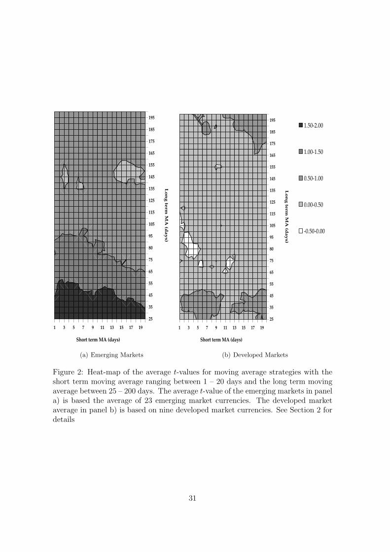
lengths of the fast and slow moving averages, we vary K between 1 – 20 days in
steps of one day and L between 25 – 200 days in steps of 5 days. Figure 2 shows the
empirical results for the individual moving average strategies based on (9) for each
13

of the resulting 720 different combinations of K and L. Panels (a) and (b) of Figure
2 show the average t-values for the 23 emerging markets currencies and for the nine
developed currencies, respectively. For the emerging markets we observe that the
average t-value of these strategies is positive for all settings. The average t-values
are high for the models with a relatively short slow moving average (L < 100),
independent of the length of the fast moving average.
The results for the developed markets are disappointing. For all settings the
t-value is between –0.5 and 1. Closer inspection of these results reveals that they
actually are poor for each of the individual developed currencies. This finding is in
line with Olson (2004), Pukthuanthong-Le et al. (2007) and Neely et al. (in press),
who report that profit opportunities for the moving average rules in the developed
currency markets disappeared by the mid-1990s.
Based on these results we decide to select all rules with a fast moving average
between 5 and 20 days and a slow moving average between 25 and 65 days, resulting
in 144 combinations of K and L. The simple average of the resulting buy-sell
signals MAt(K, L) obtained from (9) is defined as the buy-sell indicator Ct, which
is employed in the chartist trading strategy.
- insert Figure 2 and Table 4 about here -
Table 4 reports the performance statistics of the chartist strategy. The trend
strategy renders a positive return for 21 of the 23 currencies, where 10 are significant
at a 5% level. One of the best risk-adjusted results is obtained for Taiwan, with a
Sharpe ratio of 1.23 and t-statistic of 4.26. This is in line with Lee et al. (2001b),
who find that moving average technical trading rules work well for Taiwan over the
period 1988-1995. The high Sharpe ratios for Colombia, Romania and Kazakhstan
are also worth mentioning (1.23, 1.22 and 2.02 respectively), although their floating
regime history is shorter than for Taiwan. Negative returns, albeit not significant, are
found for the Mexican peso and the Sri Lanka rupee. Our findings for Mexico are in
contrast with the positive results reported by Lee et al. (2001a) for the period 1992-
99. Apart from the different sample period, this discrepancy can be explained by
the fact that Lee et al. (2001a) do not take into account the interest rate differential
in the calculation of the exchange rate returns. As seen in Table 1, with an average
14
of 12.7 percent per year the interest rate differential is far from negligible for the
Mexican peso.
Combining the individual currencies again achieves a large reduction in risk. The
equal-weighted portfolio based on the moving average trading rules has a highly eco-
nomically and statistically significant Sharpe ratio of 1.24. The Sharpe ratio further
increases to 1.52 for the volatility-weighted portfolio, as the moving average strategy
performs well for the relatively less volatile currencies (Taiwan, Peru, India, Israel
and Philippines), while it performs worse for some of the more volatile currencies
(Mexico and Czech Republic).
Trend models with daily rebalancing as considered here may lead to high turnover.
For that reason we now also consider the effects of transactions costs. Columns 6
and 7 in Table 4 show the number of transactions and the break-even transaction
costs, respectively. Averaged across individual currencies, the number of trans-
actions equals approximately 6.7 per year, which means that the chartist investor
trades about once every two months in each currency. Compared to the fundamental
strategies these numbers are rather high. For most countries and strategies having
a positive performance, break-even transaction costs exceed 0.4 percent, which for
most currencies is still above the level of transactions costs encountered in practice
by a large institutional investor.
Thus, based on our empirical analysis, we conclude that chartists may benefit
from applying a moving average trading rule in emerging markets currencies. Note
that this is not the case for the developed markets in our control sample. Although
the average return is positive for eight of the nine currencies, none of these are
significantly different from zero. Even combining the currencies into a portfolio
does not render significantly positive risk-adjusted returns, possibly as a result of
the limited diversification potential due to the high cross-correlations among these
currencies.
5 Combining fundamentalist and chartist trading
rules
In the previous two sections we analyzed the profitability of fundamentalist and
chartist investment strategies for emerging currency markets. Our empirical results
15
indicate that both types of strategies generate significantly positive risk-adjusted re-
turns over the period 1995-2007. In this section, we investigate whether the perfor-
mance can be improved further by combining fundamental and chartist information.
We start by examining a naive equally-weighted combination of both types of infor-
mation. Subsequently, this is extended to a combined strategy where the relative
weight given to fundamental and chartist signals is based on their past performance.
Table 5 shows the performance statistics of the strategy that is based on an
equally-weighted combination of the fundamental signal Ft and the chartist signal
Ct. This strategy mimics the behavior of a currency trader who puts equal value on
fundamentalist and chartist information. The benefits of combining both sources of
information is clearly borne out by the results for the individual emerging markets.
The ‘naive’ combination yields positive risk-adjusted returns for all 23 currencies,
with no less than 12 being significant at the 5 percent level. We also note that
turnover is reduced compared to the chartist strategy in Table 4, such that for most
currencies the break-even transaction costs are considerably higher than transaction
cost levels encountered in practice.
At the portfolio level, the highly significant Sharpe ratios equal 1.39 and 1.63
for the equally-weighted and volatility-weighted portfolios, respectively, which also
are higher than the Sharpe ratios for the fundamental and chartist strategies indi-
vidually. The Sharpe ratio of the combined strategy is significantly higher than the
fundamental strategy according to the Jobson and Korkie (1981) test (and Mem-
mel’s (2003) adjustment). Although the Sharpe ratio of the chartist strategy is
not significantly different from the combined strategy at the 5% level, the Jobson-
Korkie t-values of 1.80 and 1.44 for the equal and volatility weighted portfolios,
respectively, are quite high.9 This indicates that over the past 12 years an emerging
markets currency trader would have earned higher risk-adjusted returns from com-
bining fundamentalist and chartist trading rules, even with a naive equally-weighted
combination.
- insert Table 5 about here -
This result for emerging markets is in line with the questionnaire results obtained
by Taylor and Allen (1992), Lui and Mole (1998), Cheung and Chinn (2001), and
9Details are not reported here to save space, but are available upon request.
16

Gehrig and Menkhoff (2004), which indicate that foreign exchange dealers, based in
the major foreign exchange trading centers, view technical and fundamental analysis
as complementary sources of information. In contrast, a naive combination does not
seem to add sufficient value for an investor in the developed markets. We observe
that none of the individual developed currencies has a risk-adjusted return which
is statistically significant at the 5% level. Sharpe ratios are even negative (albeit
insignificant) for Canada and Norway. The equally-weighted and volatility-weighted
portfolios of developed currencies yield t-values of 1.72 and 1.60, respectively, indi-
cating that the risk-adjusted returns (0.50 and 0.46) are not significantly different
from zero.
In the heterogeneous agents models developed in Chiarella et al. (2006), De
Grauwe and Grimaldi (2005, 2006) and De Grauwe and Markiewicz (2006), agents
determine the weights assigned to the different available investment strategies based
on their relative past performance. In order to test whether this type of strategy
delivers superior returns we consider a combined investment strategy with monthly
rebalancing and dynamic weights placed on fundamental and chartist signals as
follows:
W Ft =
exp(γ
∑Jj=1 rF
t−j
)
exp(γ
∑Jj=1 rF
t−j
)+ exp
(γ
∑Kk=1 rC
t−k
) , (10)
WCt =
exp(γ
∑Jj=1 rC
t−j
)
exp(γ
∑Jj=1 rF
t−j
)+ exp
(γ
∑Jj=1 rC
t−j
) = 1−W Ft , (11)
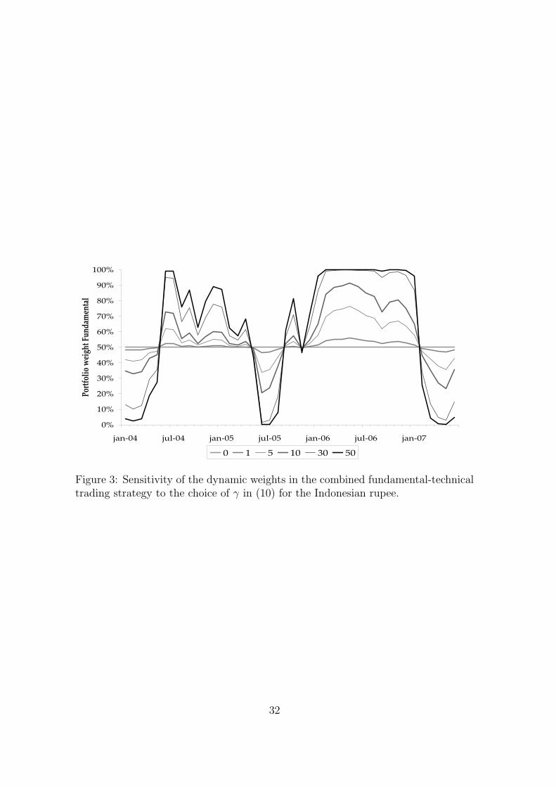
where W Ft and WC
t are the weights on the fundamentalist and chartist signals,
respectively, rFt and rC
t are the returns on the fundamentalist and chartist trading
strategies in month t, and J is the length of the look-back period of the investor.
The parameter γ ≥ 0 determines the strength of the deviation from the equally
weighted average and thus measures the ‘aggressiveness’ of the dynamic weighting
scheme. Note that the limiting case γ = 0 implies equal weighting, as this reduces
W Ft and WC
t to 0.5. Figure 3 shows an example of the sensitivity of the dynamic
weights for the choice of γ for Indonesia over the period 2004-2007.
- insert Figure 3 about here -
17

In Table 6 we display the results from the dynamic weighting scheme in (10) and
(11) with J = 12 months and γ = 30, as well as the results of our equally-weighted
strategy for the period 1997-2007.10 The results from this dynamic approach are
mixed for the individual countries, as about 2/3 of the Sharpe ratios (and their t-
values) decrease relative to the equally-weighted strategy. Nevertheless, we observe
a small increase in the level of risk-adjusted returns for both emerging market port-
folios from 1.26 and 1.53 to 1.31 and 1.59 for the equally-weighted and volatility-
weighted portfolios, respectively. This result does not depend on the particular
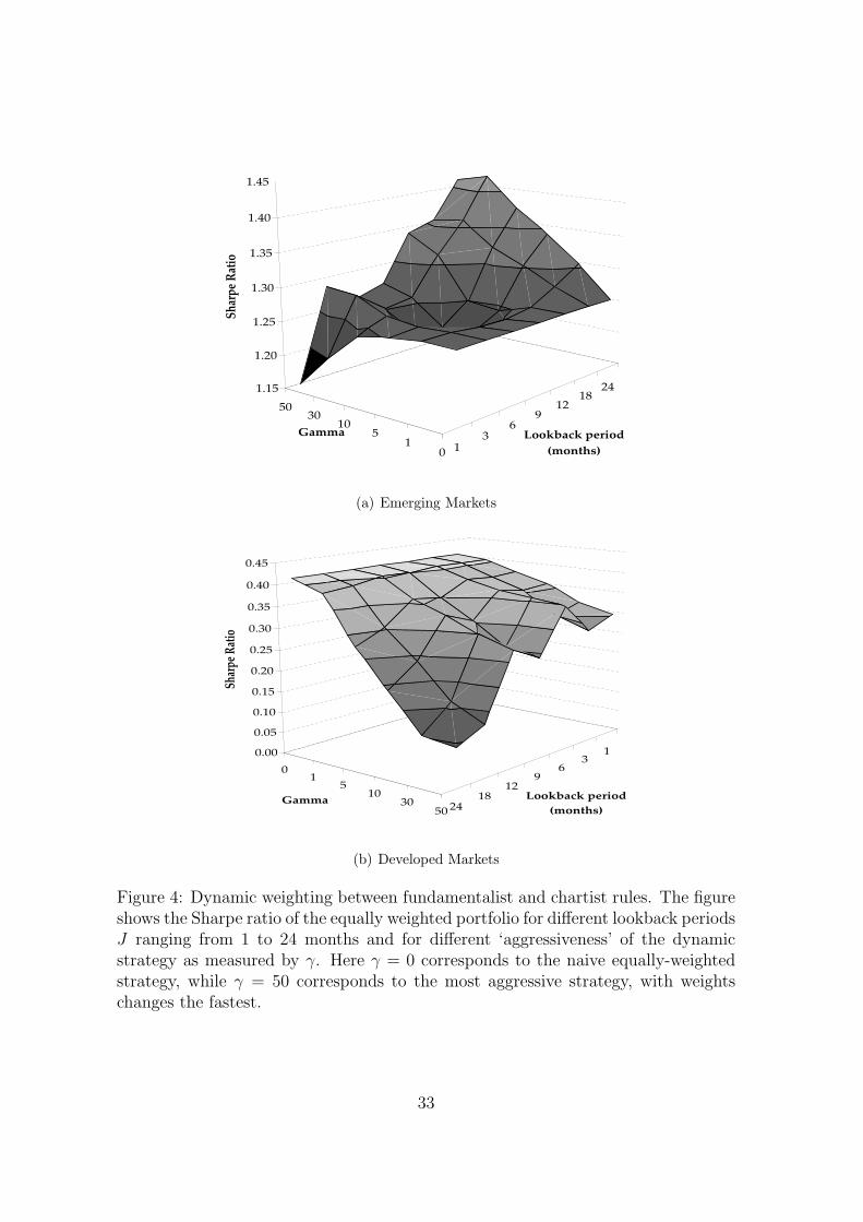
configuration of the parameters J and γ, as can be seen in Figure 4. This figure
shows the Sharpe ratios of the portfolio based on the combined strategy with dy-
namic weights for different look-back periods J ranging from 1 to 24 months and for
different levels of ‘aggressiveness’ as measured by γ. Panel (a) of Figure 4 contains
the results for the emerging markets portfolio. The Sharpe ratios are comparable for
all parameter settings, although we do observe a modest increase in the Sharpe ratio
when the look-back period gets longer and the strategy becomes more aggressive.
The difference in Sharpe ratios between the best performing dynamic strategy (with
J = 24 and γ = 50) and the equally-weighted strategy is not significant, however.11
In panel (b) of Figure 4, where we rotate the graph by 90 degrees, it can be seen
that for developed currency markets the naive equally-weighted combination seems
to be best within the range of parameters considered. The Sharpe ratio declines
along both dimensions with J or γ. This leads us to the conclusion that a dynamic
weighting scheme between chartists and fundamentalists does not yield additional
returns relative to a naive combination.
- insert Table 6 and Figure 4 about here -
6 Conclusions
Empirical research on exchange rate forecasting has tended to focus on the usefulness
of either technical analysis or of structural exchange rate models. Both question-
naires among foreign exchange market participants as well as recently developed
10We reduce the sample period to 1997-2007 such that the performance evaluation covers thesame period for all values of the look-back period J , which we vary between 1 and 24 months.
11More detailed results are available upon request.
18

heterogeneous agents models indicate that both types of information are relevant
for assessing future exchange rate movements. In addition, the heterogeneous agents
models suggest that the relative importance of chartism and fundamentalism varies
over time according to the past performance of the corresponding trading strategies.
In this paper we analyze the economic value of combining chartist and fundamen-
talist information for 23 emerging currency markets with a floating exchange rate
regime over the period 1995-2007. We document that an equally-weighted combined
chartist/fundamentalist investment strategy renders economically and statistically
significant positive risk-adjusted returns. Although both fundamentalist and chartist
trading rules individually also generate positive risk-adjusted returns on average, the
performance of the combined strategy is far superior and, in particular, much more
stable across countries. Notably, the dynamic strategy, in which the weights assigned
to chartist and fundamental information are adjusted dynamically based on relative
past performance, does not outperform a naive equally-weighted combination.
Further research can be done on the inclusion of other types of information in
the emerging currency market. More specifically, it may be of interest to expand our
information set with information on (proprietary) customer order flows of invest-
ment banks, which have been studied, as far as our knowledge, only for developed
markets, see Evans and Lyons (1999), among others. Gehrig and Menkhoff (2004),
for example, document that many foreign exchange market participants consider
flow analysis as an independent third type of information, next to technical analysis
and fundamental information. The inclusion of this additional source of information
may further increase the economic value of emerging markets currency investments.
19
References
Abhyankar, A., L. Sarno, and G. Valente (2005), Exchange rates and fundamen-
tals: evidence on the economic value of predictability, Journal of International
Economics , 66, 325–348.
Berkowitz, J. and L. Giorgianni (2001), Long-horizon exchange rate predictability,
Review of Economics and Statistics , 83, 81–91.
Brock, W. and C. Hommes (1997), A rational route to randomness, Econometrica,
65, 1059–1095.
Brock, W. and C. Hommes (1998), Heterogeneous beliefs and routes to chaos in
a simple asset pricing model, Journal of Economic Dynamics and Control , 22,
1235–1274.
Candelon, B. and S. Straetmans (2006), Testing for multiple regimes in the tail be-
havior of emerging currency returns, Journal of International Money and Finance,
25, 1187–1205.
Cheung, Y.-W. and M. D. Chinn (2001), Currency traders and exchange rate dy-
namics: a survey of the US market, Journal of International Money and Finance,
20, 439–471.
Cheung, Y.-W., M. D. Chinn, and A. G. Pascual (2005), Empirical exchange rate
models of the nineties: are any fit to survive?, Journal of International Money
and Finance, 24, 1150–1175.
Chiarella, C., X.-Z. He, and C. Hommes (2006), A dynamic analysis of moving
average rules, Journal of Economic Dynamics and Control , 30, 1729–1753.
De Grauwe, P. and M. Grimaldi (2005), Heterogeneity of agents, transactions costs,
and the exchange rate, Journal of Economic Dynamics and Control , 29, 691–719.
De Grauwe, P. and M. Grimaldi (2006), Exchange rate puzzles: a tale of switching
attractors, European Economic Review , 50, 1–33.
De Grauwe, P. and A. Markiewicz (2006), Learning to forecast the exchange rate:
Two competing approaches, CESifo Working Paper No. 1717.
20

De Jong, E., W. F. Verschoor, and R. C. J. Zwinkels (2006), Heterogeneity of agents
and excange rate dynamics: evidence from the EMS, Radboud University, working
paper.
Evans, M. and R. K. Lyons (1999), Order flow and exchange rate dynamics, Journal
of Political Economy , 110, 170–180.
Frankel, J. A. (1979), On the Mark: a theory of floating exchange rates based on
real interest differentials, American Economic Review , 69, 610–622.
Frankel, J. A. and K. A. Froot (1990), Chartists, fundamentalists, and trading in
the foreign exchange market, American Economic Review , 80, 181–185.
Gehrig, T. and L. Menkhoff (2004), The use of flow analysis in foreign exchange:
exploratory evidence, Journal of International Money and Finance, 23, 573–594.
Isaac, A. G. and S. de Mel (2001), The real-interest-differential model after 20 years,
Journal of International Money and Finance, 20, 473–495.
Jobson, J. and B. Korkie (1981), Performance hypothesis testing with the Sharpe
and Treynor measures, Journal of Finance, 36, 889–908.
Kaminsky, G. L. (2006), Currency crisis: are they all the same?, Journal of Inter-
national Money and Finance, 25, 503–527.
Kilian, L. (2001), Exchange rates and fundamentals: What do we learn from long-
horizon regressions?, Journal of Applied Econometrics , 14, 491–510.
LeBaron, B. (1999), Technical trading rule profitability and foreign exchange inter-
vention, Journal of International Economics , 49, 125–143.
Lee, C. I., K. C. Gleason, and I. Mathur (2001a), Trading rule profits in Latin
American currency spot rates, International Review of Financial Analysis , 10,
135–156.
Lee, C. I., M.-S. Pan, and Y. A. Liu (2001b), On market efficiency of Asian foreign
exchange rates: Evidence from a joint variance ratio test and technical trading
rules, Journal of International Financial Markets, Institutions and Money , 11,
199–214.
21
Leitch, G. and J. E. Tanner (1991), Economic forecast evaluation: profits versus the
conventional error measures, American Economic Review , 81, 580–590.
Levich, R. and L. Thomas (1993), The significance of technical trading rule profits
in the foreign exchange market: a bootstrap approach, Journal of International
Money and Finance, 12, 451–474.
Lui, Y. and D. Mole (1998), The use of fundamental and technical analyses by
foreign exchange dealers: Hong Kong evidence, Journal of International Money
and Finance, 17, 535–545.
Mark, N. C. (1995), Exchange rates and fundamentals: Evidence on long-horizon
predictability, American Economic Review , 85, 201–218.
Martin, A. D. (2001), Technical trading rules in the spot foreign exchange markets of
developing countries, Journal of Multinational Financial Management , 11, 59–68.
McNown, R. and M. Wallace (1989), National price levels, purchasing power parity,
and cointegration: a test of four high inflation economies, Journal of International
Money and Finance, 8, 533–545.
Meese, R. and K. Rogoff (1983), Empirical exchange rate models of the seventies:
do they fit out-of-sample?, Journal of International Economics , 14, 3–24.
Memmel, C. (2003), Performance hypothesis testing with the Sharpe ratio, Finance
Letters , 1, 21–23.
Menkhoff, L. (1997), Examining the use of technical currency analysis, Journal of
Economic Literature, 2, 307–318.
Menkhoff, L. and M. P. Taylor (2007), The obstinate passion of foreign exchange
professionals: Technical analysis, Journal of Economic Literature, 45, 936–972.
Neely, C. J. and P. A. Weller (1999), Technical trading rules in the European Mon-
etary System, Journal of International Money and Finance, 18, 429–458.
Neely, C. J., P. A. Weller, and J. M. Ulrich (in press), The adaptive markets hy-
pothesis: evidence from the foreign exchange market, Journal of Financial and
Quantitative Analysis .
22
Olson, D. (2004), Have trading rule profits in the currency markets declined over
time?, Journal of Banking and Finance, 28, 85–105.
Pukthuanthong-Le, K., R. M. Levich, and L. R. Thomas (2007), Do foreign exchange
markets still trend?, Journal of Portfolio Management , 34, 114–118.
Sullivan, R., A. Timmermann, and H. White (1999), Data-snooping, technical trad-
ing rule performance and the bootstrap, Journal of Finance, 54, 1647–1691.
Sweeney, R. (1986), Beating the foreign exchange market, Journal of Finance, 41,
163–182.
Taylor, M. P. and H. Allen (1992), The use of technical analysis in the foreign
exchange market, Journal of International Money and Finance, 11, 304–314.
Vigfusson, R. (1997), Switching between chartists and fundamentalists: a Markov
regime-switching approach, International Journal of Financial Economics , 2, 291–
305.
23

Table 1: Summary statistics currency returns
Currency Float Mean Stdev Skew. Kurt. FX IRDEmergingTaiwanese dollar (TWD) Dec-94 2.45 5.52 0.06 5.43 1.9 0.6Peruvian sol (PEN) Dec-94 −3.17 4.00 −0.12 4.12 2.7 −5.8Indian rupee (INR) Dec-94 0.04 5.05 0.74 5.13 2.0 −1.9Mexican peso (MXN) Dec-94 −8.23 9.06 0.53 1.68 4.4 −12.7S. African rand (ZAR) Jan-95 −2.07 15.37 0.20 1.21 5.5 −7.6Czech koruna (CZK) May-97 −5.45 11.57 −0.27 −0.20 −4.5 −1.0Israeli shekel (ILS) Jun-97 −1.82 7.41 1.45 5.46 1.9 −3.8Thai bath (THB) Jul-97 −3.55 11.97 −2.43 18.33 −3.3 −0.3Phillipine peso (PHP) Jul-97 −4.70 8.43 −0.05 4.43 1.4 −6.1Indonesian rupiah (IDR) Aug-97 −11.97 26.49 −0.64 8.83 0.4 −12.3Korean won (KRW) Dec-97 −5.47 9.60 −0.14 4.58 −4.6 −0.8Slovak koruna (SKK) Oct-98 −8.92 10.26 −0.24 −0.29 −6.2 −2.7Brazilian real (BRL) Feb-99 −13.31 17.61 1.10 5.24 0.9 −14.2Chilean peso (CLP) Sep-99 0.19 9.27 −0.14 −0.34 0.7 −0.5Colombian peso (COP) Sep-99 −5.05 9.14 −0.12 3.30 0.1 −5.1Polish zloty (PLN) Apr-00 −11.80 11.01 0.08 −0.30 −7.1 −4.7Turkish lira (TRY) Feb-01 −25.64 16.68 0.34 1.93 −0.2 −25.4Hungarian forint (HUF) May-01 −13.45 12.02 0.59 1.16 −7.7 −5.7Sri Lanka rupee (LKR) Dec-01 −4.59 3.92 −1.39 9.41 2.9 −7.5Argentine peso (ARS) Jan-02 −13.77 9.28 −1.38 2.40 −4.1 −9.6Romanian leu (RON) Oct-04 −9.85 8.93 0.17 −0.90 −8.0 −1.9Kazakhstan tenge (KZT) Dec-04 −5.09 6.40 1.21 3.65 −4.1 −1.0Malaysian ringitt (MYR) Jul-05 −4.41 3.44 0.43 0.19 −6.0 1.6
DevelopedAustralian dollar (AUD) Dec-94 −2.59 9.88 0.21 −0.04 −1.3 −1.2Canadian dollar (CAD) Dec-94 −1.84 6.33 −0.09 0.01 −2.1 0.3UK sterling (GBP) Dec-94 −3.04 7.26 0.03 −0.14 −1.9 −1.1Japanese yen (JPY) Dec-94 7.13 11.02 −0.88 4.72 3.1 4.0Euro (EUR/DEM) Dec-94 1.31 9.37 −0.25 0.06 0.2 1.1Swiss franc (CHF) Dec-94 3.14 9.87 −0.28 −0.39 0.5 2.7Norwegian krone (NOK) Dec-94 −0.99 9.99 −0.12 0.58 −0.5 −0.5Swedish krona (SEK) Dec-94 −0.14 10.13 −0.31 −0.01 −0.5 0.4N. Zealand dollar (NZD) Dec-94 −3.70 10.58 0.28 0.43 −1.3 −2.4
Note: The table shows annualized statistics (mean, standard deviation, skewness and kurtosis) ofmonthly returns on 23 emerging markets and 9 developed market foreign exchange rates (based on along US dollar position and a short position in the emerging market) for the period January 1995 -June 2007. The returns include the spot rate change as well as the interest rate differential betweenthe US and the specific country. Columns 7-8 report the average, annualized return on the foreignexchange rate (FX) and the average, annualized interest rate differential (IRD), respectively.
24
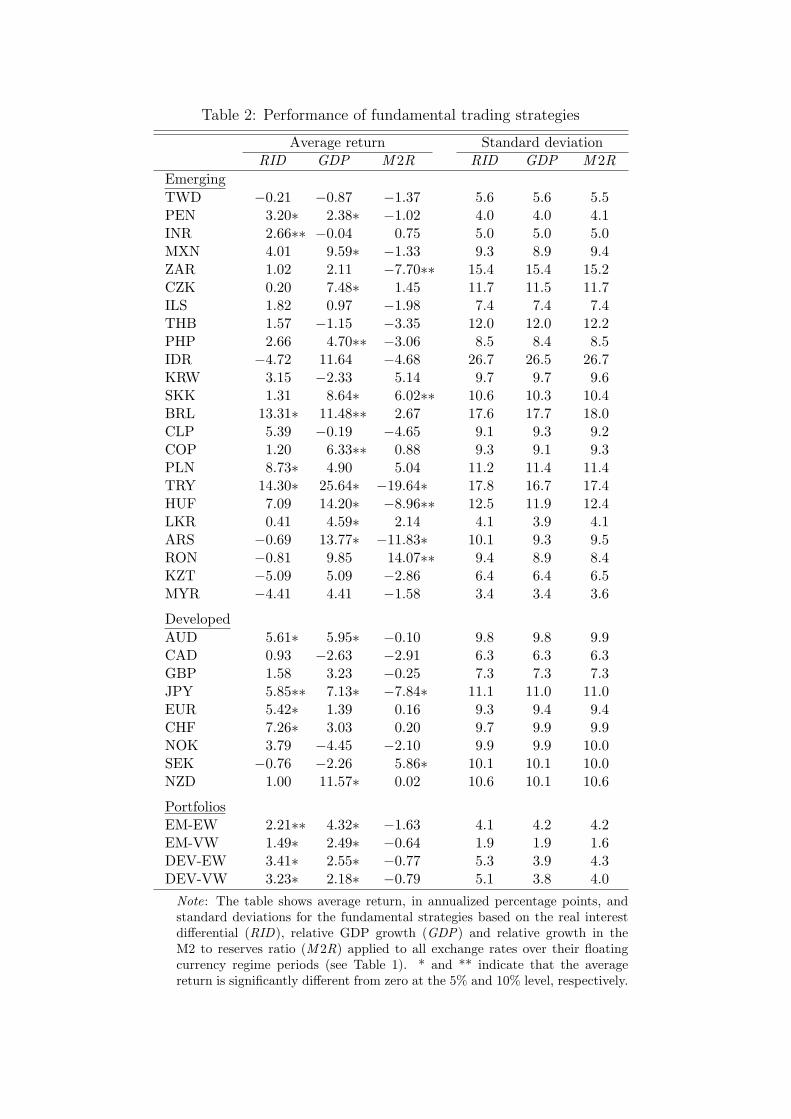
Table 2: Performance of fundamental trading strategies
Average return Standard deviationRID GDP M 2R RID GDP M 2R
EmergingTWD −0.21 −0.87 −1.37 5.6 5.6 5.5PEN 3.20∗ 2.38∗ −1.02 4.0 4.0 4.1INR 2.66∗∗ −0.04 0.75 5.0 5.0 5.0MXN 4.01 9.59∗ −1.33 9.3 8.9 9.4ZAR 1.02 2.11 −7.70∗∗ 15.4 15.4 15.2CZK 0.20 7.48∗ 1.45 11.7 11.5 11.7ILS 1.82 0.97 −1.98 7.4 7.4 7.4THB 1.57 −1.15 −3.35 12.0 12.0 12.2PHP 2.66 4.70∗∗ −3.06 8.5 8.4 8.5IDR −4.72 11.64 −4.68 26.7 26.5 26.7KRW 3.15 −2.33 5.14 9.7 9.7 9.6SKK 1.31 8.64∗ 6.02∗∗ 10.6 10.3 10.4BRL 13.31∗ 11.48∗∗ 2.67 17.6 17.7 18.0CLP 5.39 −0.19 −4.65 9.1 9.3 9.2COP 1.20 6.33∗∗ 0.88 9.3 9.1 9.3PLN 8.73∗ 4.90 5.04 11.2 11.4 11.4TRY 14.30∗ 25.64∗ −19.64∗ 17.8 16.7 17.4HUF 7.09 14.20∗ −8.96∗∗ 12.5 11.9 12.4LKR 0.41 4.59∗ 2.14 4.1 3.9 4.1ARS −0.69 13.77∗ −11.83∗ 10.1 9.3 9.5RON −0.81 9.85 14.07∗∗ 9.4 8.9 8.4KZT −5.09 5.09 −2.86 6.4 6.4 6.5MYR −4.41 4.41 −1.58 3.4 3.4 3.6
DevelopedAUD 5.61∗ 5.95∗ −0.10 9.8 9.8 9.9CAD 0.93 −2.63 −2.91 6.3 6.3 6.3GBP 1.58 3.23 −0.25 7.3 7.3 7.3JPY 5.85∗∗ 7.13∗ −7.84∗ 11.1 11.0 11.0EUR 5.42∗ 1.39 0.16 9.3 9.4 9.4CHF 7.26∗ 3.03 0.20 9.7 9.9 9.9NOK 3.79 −4.45 −2.10 9.9 9.9 10.0SEK −0.76 −2.26 5.86∗ 10.1 10.1 10.0NZD 1.00 11.57∗ 0.02 10.6 10.1 10.6
PortfoliosEM-EW 2.21∗∗ 4.32∗ −1.63 4.1 4.2 4.2EM-VW 1.49∗ 2.49∗ −0.64 1.9 1.9 1.6DEV-EW 3.41∗ 2.55∗ −0.77 5.3 3.9 4.3DEV-VW 3.23∗ 2.18∗ −0.79 5.1 3.8 4.0
Note: The table shows average return, in annualized percentage points, andstandard deviations for the fundamental strategies based on the real interestdifferential (RID), relative GDP growth (GDP) and relative growth in theM2 to reserves ratio (M 2R) applied to all exchange rates over their floatingcurrency regime periods (see Table 1). * and ** indicate that the averagereturn is significantly different from zero at the 5% and 10% level, respectively.
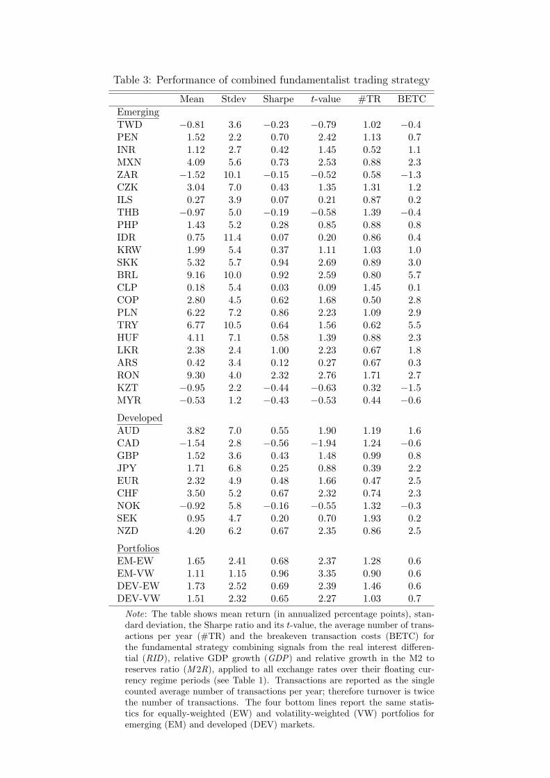
Table 3: Performance of combined fundamentalist trading strategy
Mean Stdev Sharpe t-value #TR BETCEmergingTWD −0.81 3.6 −0.23 −0.79 1.02 −0.4PEN 1.52 2.2 0.70 2.42 1.13 0.7INR 1.12 2.7 0.42 1.45 0.52 1.1MXN 4.09 5.6 0.73 2.53 0.88 2.3ZAR −1.52 10.1 −0.15 −0.52 0.58 −1.3CZK 3.04 7.0 0.43 1.35 1.31 1.2ILS 0.27 3.9 0.07 0.21 0.87 0.2THB −0.97 5.0 −0.19 −0.58 1.39 −0.4PHP 1.43 5.2 0.28 0.85 0.88 0.8IDR 0.75 11.4 0.07 0.20 0.86 0.4KRW 1.99 5.4 0.37 1.11 1.03 1.0SKK 5.32 5.7 0.94 2.69 0.89 3.0BRL 9.16 10.0 0.92 2.59 0.80 5.7CLP 0.18 5.4 0.03 0.09 1.45 0.1COP 2.80 4.5 0.62 1.68 0.50 2.8PLN 6.22 7.2 0.86 2.23 1.09 2.9TRY 6.77 10.5 0.64 1.56 0.62 5.5HUF 4.11 7.1 0.58 1.39 0.88 2.3LKR 2.38 2.4 1.00 2.23 0.67 1.8ARS 0.42 3.4 0.12 0.27 0.67 0.3RON 9.30 4.0 2.32 2.76 1.71 2.7KZT −0.95 2.2 −0.44 −0.63 0.32 −1.5MYR −0.53 1.2 −0.43 −0.53 0.44 −0.6
DevelopedAUD 3.82 7.0 0.55 1.90 1.19 1.6CAD −1.54 2.8 −0.56 −1.94 1.24 −0.6GBP 1.52 3.6 0.43 1.48 0.99 0.8JPY 1.71 6.8 0.25 0.88 0.39 2.2EUR 2.32 4.9 0.48 1.66 0.47 2.5CHF 3.50 5.2 0.67 2.32 0.74 2.3NOK −0.92 5.8 −0.16 −0.55 1.32 −0.3SEK 0.95 4.7 0.20 0.70 1.93 0.2NZD 4.20 6.2 0.67 2.35 0.86 2.5
PortfoliosEM-EW 1.65 2.41 0.68 2.37 1.28 0.6EM-VW 1.11 1.15 0.96 3.35 0.90 0.6DEV-EW 1.73 2.52 0.69 2.39 1.46 0.6DEV-VW 1.51 2.32 0.65 2.27 1.03 0.7
Note: The table shows mean return (in annualized percentage points), stan-dard deviation, the Sharpe ratio and its t-value, the average number of trans-actions per year (#TR) and the breakeven transaction costs (BETC) forthe fundamental strategy combining signals from the real interest differen-tial (RID), relative GDP growth (GDP) and relative growth in the M2 toreserves ratio (M 2R), applied to all exchange rates over their floating cur-rency regime periods (see Table 1). Transactions are reported as the singlecounted average number of transactions per year; therefore turnover is twicethe number of transactions. The four bottom lines report the same statis-tics for equally-weighted (EW) and volatility-weighted (VW) portfolios foremerging (EM) and developed (DEV) markets.
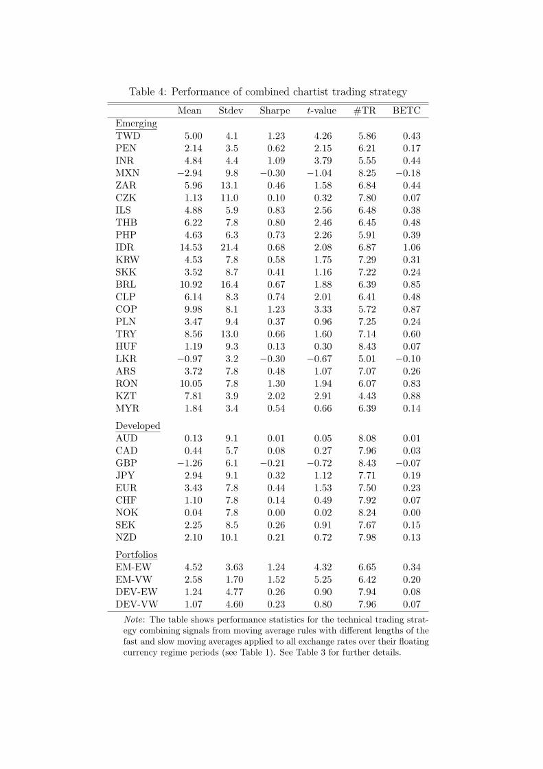
Table 4: Performance of combined chartist trading strategy
Mean Stdev Sharpe t-value #TR BETCEmergingTWD 5.00 4.1 1.23 4.26 5.86 0.43PEN 2.14 3.5 0.62 2.15 6.21 0.17INR 4.84 4.4 1.09 3.79 5.55 0.44MXN −2.94 9.8 −0.30 −1.04 8.25 −0.18ZAR 5.96 13.1 0.46 1.58 6.84 0.44CZK 1.13 11.0 0.10 0.32 7.80 0.07ILS 4.88 5.9 0.83 2.56 6.48 0.38THB 6.22 7.8 0.80 2.46 6.45 0.48PHP 4.63 6.3 0.73 2.26 5.91 0.39IDR 14.53 21.4 0.68 2.08 6.87 1.06KRW 4.53 7.8 0.58 1.75 7.29 0.31SKK 3.52 8.7 0.41 1.16 7.22 0.24BRL 10.92 16.4 0.67 1.88 6.39 0.85CLP 6.14 8.3 0.74 2.01 6.41 0.48COP 9.98 8.1 1.23 3.33 5.72 0.87PLN 3.47 9.4 0.37 0.96 7.25 0.24TRY 8.56 13.0 0.66 1.60 7.14 0.60HUF 1.19 9.3 0.13 0.30 8.43 0.07LKR −0.97 3.2 −0.30 −0.67 5.01 −0.10ARS 3.72 7.8 0.48 1.07 7.07 0.26RON 10.05 7.8 1.30 1.94 6.07 0.83KZT 7.81 3.9 2.02 2.91 4.43 0.88MYR 1.84 3.4 0.54 0.66 6.39 0.14
DevelopedAUD 0.13 9.1 0.01 0.05 8.08 0.01CAD 0.44 5.7 0.08 0.27 7.96 0.03GBP −1.26 6.1 −0.21 −0.72 8.43 −0.07JPY 2.94 9.1 0.32 1.12 7.71 0.19EUR 3.43 7.8 0.44 1.53 7.50 0.23CHF 1.10 7.8 0.14 0.49 7.92 0.07NOK 0.04 7.8 0.00 0.02 8.24 0.00SEK 2.25 8.5 0.26 0.91 7.67 0.15NZD 2.10 10.1 0.21 0.72 7.98 0.13
PortfoliosEM-EW 4.52 3.63 1.24 4.32 6.65 0.34EM-VW 2.58 1.70 1.52 5.25 6.42 0.20DEV-EW 1.24 4.77 0.26 0.90 7.94 0.08DEV-VW 1.07 4.60 0.23 0.80 7.96 0.07
Note: The table shows performance statistics for the technical trading strat-egy combining signals from moving average rules with different lengths of thefast and slow moving averages applied to all exchange rates over their floatingcurrency regime periods (see Table 1). See Table 3 for further details.

Table 5: Performance of equally-weighted fundamentalist-chartisttrading strategy
Mean Stdev Sharpe t-value #TR BETCEmergingTWD 2.09 2.63 0.80 2.77 3.44 0.30PEN 1.83 2.12 0.87 3.01 3.67 0.25INR 2.98 2.83 1.06 3.67 3.04 0.49MXN 0.57 5.35 0.11 0.37 4.57 0.06ZAR 2.22 7.75 0.29 0.99 3.71 0.30CZK 2.09 7.07 0.30 0.92 4.55 0.23ILS 2.57 3.13 0.82 2.54 3.67 0.35THB 2.72 4.38 0.62 1.87 3.92 0.35PHP 3.03 3.34 0.91 2.79 3.39 0.45IDR 7.70 11.11 0.69 2.12 3.86 1.00KRW 3.26 5.29 0.62 1.86 4.16 0.39SKK 4.42 5.46 0.81 2.33 4.06 0.54BRL 10.04 9.10 1.10 3.10 3.59 1.40CLP 3.16 5.05 0.63 1.69 3.93 0.40COP 6.39 4.67 1.37 3.70 3.11 1.03PLN 4.85 6.83 0.71 1.84 4.17 0.58TRY 7.67 8.47 0.91 2.20 3.88 0.99HUF 2.65 6.65 0.40 0.95 4.66 0.28LKR 0.70 1.99 0.35 0.79 2.84 0.12ARS 2.07 3.08 0.67 1.51 3.87 0.27RON 10.48 5.83 1.80 2.14 3.89 1.35KZT 3.43 2.36 1.45 2.10 2.38 0.72MYR 0.66 1.65 0.40 0.48 3.41 0.10
DevelopedAUD 1.98 6.20 0.32 1.11 4.63 0.21CAD −0.55 2.80 −0.20 −0.68 4.60 −0.06GBP 0.13 4.06 0.03 0.11 4.71 0.01JPY 2.33 5.32 0.44 1.52 4.05 0.29EUR 2.88 5.14 0.56 1.95 3.98 0.36CHF 2.30 5.10 0.45 1.57 4.33 0.27NOK −0.44 5.00 −0.09 −0.31 4.78 −0.05SEK 1.60 5.04 0.32 1.10 4.80 0.17NZD 3.15 6.48 0.49 1.69 4.42 0.36
PortfoliosEM-EW 3.08 2.22 1.39 4.81 3.97 0.39EM-VW 1.83 1.12 1.63 5.65 3.66 0.25DEV-EW 1.48 2.98 0.50 1.72 4.70 0.16DEV-VW 1.30 2.83 0.46 1.60 4.50 0.15
Note: The table shows performance statistics for the equally-weightedfundamentalist-chartist strategy applied to all exchange rates over their float-ing currency regime periods (see Table 1). See Table 3 for further details.

Table 6: Performance of dynamic combined fundamentalist-chartist trading strategy
Dynamic weights Equally-weightedMean Stdev Sharpe t-value Mean Stdev Sharpe t-value
EmergingTWD 4.49 3.78 1.19 3.78 2.37 2.69 0.88 2.80PEN 2.51 2.68 0.94 2.98 2.38 2.22 1.07 3.41INR 3.78 3.17 1.19 3.79 3.12 2.60 1.20 3.81MXN 0.05 8.19 0.01 0.02 −0.41 5.35 −0.08 −0.24ZAR 5.29 13.81 0.38 1.21 2.18 8.40 0.26 0.82CZK 1.83 7.00 0.26 0.72 3.12 6.72 0.46 1.29ILS 1.99 3.91 0.51 1.40 2.62 3.16 0.83 2.29THB 4.97 4.79 1.04 2.76 3.38 3.18 1.06 2.83PHP 4.37 5.17 0.85 2.32 2.80 2.48 1.13 3.09IDR 6.72 9.32 0.72 1.96 4.39 6.74 0.65 1.77KRW 1.91 4.80 0.40 1.06 3.12 4.37 0.71 1.90SKK 6.28 6.60 0.95 2.38 4.98 5.65 0.88 2.20BRL 13.58 16.72 0.81 1.98 11.35 9.87 1.15 2.80CLP 3.91 7.05 0.55 1.28 2.79 5.24 0.53 1.23COP 7.62 6.51 1.17 2.70 6.98 5.18 1.35 3.11PLN 1.58 6.77 0.23 0.51 4.42 6.82 0.65 1.41TRY 4.88 10.93 0.45 0.88 7.37 7.13 1.03 2.05HUF 1.13 5.28 0.21 0.41 1.00 5.75 0.17 0.33LKR −0.80 1.32 −0.60 −1.05 −0.60 1.59 −0.38 −0.65ARS 0.27 1.43 0.19 0.33 0.53 1.48 0.35 0.61RON 22.60 5.74 3.94 1.97 23.24 5.78 4.02 2.01KZT NA NA NA NA NA NA NA NAMYR NA NA NA NA NA NA NA NA
DevelopedAUD 3.21 7.98 0.40 1.28 2.44 6.67 0.37 1.16CAD −0.72 4.47 −0.16 −0.51 −0.48 2.92 −0.17 −0.52GBP 0.02 3.85 0.00 0.01 0.11 3.87 0.03 0.09JPY 0.56 5.86 0.10 0.30 0.96 4.79 0.20 0.64EUR 2.20 5.56 0.39 1.25 2.98 5.22 0.57 1.81CHF 0.58 5.63 0.10 0.33 1.47 4.62 0.32 1.01NOK 0.43 6.48 0.07 0.21 −0.29 5.12 −0.06 −0.18SEK 0.46 6.08 0.08 0.24 1.01 4.79 0.21 0.67NZD 2.78 8.18 0.34 1.08 3.32 7.01 0.47 1.50
PortfoliosEM-EW 3.83 2.91 1.31 4.17 2.78 2.21 1.26 3.99EM-VW 1.93 1.21 1.59 5.06 1.61 1.05 1.53 4.86DEV-EW 1.06 3.54 0.30 0.95 1.28 3.12 0.41 1.30DEV-VW 0.92 3.39 0.27 0.86 1.14 2.97 0.38 1.21
Note: The table shows performance statistics for the combined fundamentalist-chartist strategywith weights determined by the relative performance during the past 12 months, applied to allexchange rates over their floating currency regime periods in the period 1997-2007 (see Table1). See Table 3 for further details.
0
5
10
15
20
25
dec-94 dec-96 dec-98 dec-00 dec-02 dec-04 dec-06
Nu
mb
er
of
cou
ntr
ies
Figure 1: Number of emerging market countries with floating exchange rate regime,December 1994 – June 2007.
30
1 3 5 7 9 11 13 15 17 19
25
35
45
55
65
75
80
95
105
115
125
135
145
155
165
175
185
195
Short term MA (days)
Lo
ng
te
rm
MA
(d
ay
s)
(a) Emerging Markets
1 3 5 7 9 11 13 15 17 19
25
35
45
55
65
75
80
95
105
115
125
135
145
155
165
175
185
195
Short term MA (days)
Lo
ng
te
rm
MA
(d
ay
s)
1.50-2.00
1.00-1.50
0.50-1.00
0.00-0.50
-0.50-0.00
(b) Developed Markets
Figure 2: Heat-map of the average t-values for moving average strategies with theshort term moving average ranging between 1 – 20 days and the long term movingaverage between 25 – 200 days. The average t-value of the emerging markets in panela) is based the average of 23 emerging market currencies. The developed marketaverage in panel b) is based on nine developed market currencies. See Section 2 fordetails
31
0%
10%
20%
30%
40%
50%
60%
70%
80%
90%
100%
jan-04 jul-04 jan-05 jul-05 jan-06 jul-06 jan-07
Po
rtfo
lio
we
igh
t F
un
da
me
nta
l
0 1 5 10 30 50
Figure 3: Sensitivity of the dynamic weights in the combined fundamental-technicaltrading strategy to the choice of γ in (10) for the Indonesian rupee.
32
1
3
6
912
1824
01
510
3050
1.15
1.20
1.25
1.30
1.35
1.40
1.45
Sh
arp
e R
ati
o
Lookback period
(months)
Gamma
(a) Emerging Markets
13
69
12
18
24
01
510
3050
0.00
0.05
0.10
0.15
0.20
0.25
0.30
0.35
0.40
0.45
Sh
arp
e R
atio
Lookback period
(months)
Gamma
(b) Developed Markets
Figure 4: Dynamic weighting between fundamentalist and chartist rules. The figureshows the Sharpe ratio of the equally weighted portfolio for different lookback periodsJ ranging from 1 to 24 months and for different ‘aggressiveness’ of the dynamicstrategy as measured by γ. Here γ = 0 corresponds to the naive equally-weightedstrategy, while γ = 50 corresponds to the most aggressive strategy, with weightschanges the fastest.
33


