1
The G-Econ Database on Gridded Output: Methods and Data1
William Nordhaus, Qazi Azam, David Corderi, Kyle Hood, Nadejda Makarova
Victor, Mukhtar Mohammed, Alexandra Miltner, and Jyldyz Weiss2
Yale University May 12, 2006
Abstract
The present study describes a project that has developed a geophysically based data set on economic activity. The project is called the Yale G-Econ project (for Geographically based Economic data). The G-Econ data set calculates gross value added at a 1-degree longitude by 1-degree latitude resolution at a global scale for all terrestrial cells. These data allow better integration of economic and environmental data to investigate environmental economics, the impact of global warming, and the role of geophysical factors in economic activity. On of the major results is to show that the true economic deserts of the globe are in Greenland, Antarctica, northern Canada, Alaska, and Siberia.
1 This research was supported by the National Science Foundation and the Glaser Foundation. Nordhaus is primarily responsible for this report. The underlying data for G-
Econ 1.3 as of May 2006 can be found at the project web site at gecon.yale.edu.2 Nordhaus is Sterling Professor of Economics, Yale University, 28 Hillhouse
Avenue, New Haven, CT, 06511, email [email protected], and is corresponding author. Azam was Associate in Research, Department of Economics, Yale University, project associate 2003-2005. Corderi was Associate in Research, Department of Economics, Yale University, project associate 2005-06. Corderi was a graduate student in Economics, Yale University and project associate 2003-06. Victor is Fellow at the Program on Energy and Sustainable Development at Stanford University and was project associate 2000-2004. Mohammed was Associate in Research, Department of Economics, Yale University, project associate 2003-2005. Miltner was Associate in Research, Department of Economics, Yale University, project associate 2001-2003. Weiss was Associate in Research, Department of Economics, Yale University, project associate 2005-06.
2
I. Introduction
The last two decades have witnessed a dramatic growth in interest, at both
national and international levels, in geography and geophysical data. A major hurdle
for current research is the complete disjunction of socioeconomic and geophysical
analyses. In part, the lack of intersection of the research programs has been due to the
disparate interests and descriptions of the different disciplines working in these two
areas.
One group of studies has been largely undertaken by economists and other
social scientists concerned with “wealth of nations,” comparative growth rates, and
national economic policies. These analyses have naturally relied upon socioeconomic
data constructed from accounts largely free of any geophysical dimension and sorted
by political boundaries. Economic studies of the relationship between economic
activity and geography have generally relied upon data that are organized by political
jurisdictions (countries, states, counties, and the like). Most recent analysis has
debated the relative importance of geography, institutions, and leadership in
determining income patterns.3
3 For example, see R.E. Hall and C. I. Jones Hall (1999) “Why Do Some Countries Produce So Much More Output Per Worker Than Others?” Quarterly Journal Economics, 114 , 1, pp. 83-116.; J. D. Sachs, A. Mellinger, and J. Gallup (2000), “Climate, Coastal Proximity, and Development,” in Gordon L. Clark, G.L., Feldman, M. P., and Gertler, M. S., eds., Oxford Handbook of Economic Geography (Oxford University Press, Oxford, UK; D. Acemoglu, S. Johnson, and J. A. Robinson, J. A (2001) “The Colonial Origins of Comparative Development: An Empirical Investigation,” American Economic Review, 91, pp. 1369-1401.
3
The other group of studies, largely undertaken by natural scientists, has
concentrated on understanding geophysical processes. These have increasingly relied
upon terrestrial or satellite observation of a variety of geophysical phenomena such as
weather or climate, ecological features, soils, glaciology, and so forth. The units of
analysis in these geophysical studies are generally physical, or “gridded” by latitude
or longitude. Prominent examples of such geophysically-based studies are ones that
project the climatic consequences of the accumulation of radiatively active
atmospheric gases. 4 There have been several attempts to link geophysical studies with
socioeconomic studies. Perhaps the most intensive have been the “integrated
assessment” models developed in the climate-change community.5 These analyses
have invariably linked the geophysical and socioeconomic modules by rescaling the
geophysical variables (such as climate and ecological impacts) into political
boundaries.
There have been few attempts to rescale from political to geophysical scaling.
This gap has occurred partly because the major impacts being examined were
economic ones along with national economic or energy policies. Even more important,
however, has been the complete lack of an integrated socioeconomic database scaled
on a geophysical level. To put it simply, it would be impossible to conduct an
4 There is a vast literature on the impact of industrial activity on climate. A systematic review is contained in J.T. Houghton, Y. Ding, D.J. Griggs, M. Noguer, P.J. van der Linden, X. Dai, K. Maskell, and C.A. Johnson (2001), eds., Climate Change 2001: The Scientific Basis, Cambridge University Press, Cambridge, UK.
5 See W. D. Nordhaus, and J. Boyer (2000), Warming the World: Economic Modeling of Global Warming, MIT Press, Cambridge, MA. A review of existing integrated assessment models is contained in Bruce, J.P., Lee, H., and Haites, E.F., eds. (1995) Climate Change 1995: Economic and Social Dimensions of Climate Change, Cambridge University Press, UK, chapter 10.
4
economic analysis on a geophysical basis today because the underlying data do not
currently exist.
The present study describes the results of a project to develop a
geophysically based data set on economic activity. The project is called the Yale
G-Econ project (for Geographically based Economic data). The G-Econ data
presented here estimate gross output at a 1-degree longitude by 1-degree latitude
resolution at a global scale. This includes virtually all terrestrial regions. The
resolution is approximately 100 km by 100 km, which is approximately the size of
most third-level political entities (e.g., counties in the United States). The effort is
limited to producing data on value added (conceptually similar to gross domestic
product) for 1990. In the course of the study, we have also developed or relied
upon data on population, land area, some estimates of minerals production, and
“RIG” or area of a region or country within each grid cell. For all countries, we
have developed output measures converted into common metrics using both
market exchange rates and purchasing power parity (PPP) exchange rates. For
some countries, we develop more detailed data (for example, we have developed
data by grid cell and major industry for decades from 1950 to 2000 for the United
States), but these data are not yet available for general use.
There are several advantages of the G-Econ data set for studies in economic
geography and environmental economics. One important advantage is that it can
easily link economic data to readily available geophysical data (such as on
climate, soils, ecology, and the like). A second advantage is that the database for
studying global processes is much more detailed than the standard ones. By
disaggregating to grid cells, the number of useful observations increases from
around 100 countries to over 27,000 terrestrial cells. Additionally, because the

5
data set has multiple observations per country, it is possible to control for factors
that are unique to individual countries.
In addition to the level of aggregation, the G-Econ data set emphasizes
certain features that are unavailable in conventional approaches. First, the data
are primarily concerned with the geographical intensity of economic activity rather
than the personal intensity of economic activity. In other words, the data focus on
the intensity of economic activity per unit area rather than per capita or per hour
worked. This approach places the emphasis clearly on geography rather than
demography. Second, by emphasizing gridded data rather than national data,
this data set allows a much richer set of geophysical data to be used in the
analysis. Most of the important geographical data (climate, location, distance
from markets or seacoasts, soils, and so forth) are generally collated on a
geophysical basis rather than based on political boundaries. There is also an
important interaction between the finer resolution of the economic data and the
use of geophysical data because, for many countries, averages of many variables
(such as temperature or distance from seacoast) cover such a huge area that they
are virtually meaningless, whereas for most grid cells the averages cover a
reasonably small area.
6
II. Methodology for Estimating Gross Cell Product
Gross Cell Product
The major statistical contribution of the present research program has been
the development of “gridded output” data, which are called gross cell product or
GCP. The conceptual basis of GCP is the same as gross domestic product (GDP) as
developed in the national income and product accounts of major countries. These
procedures have been harmonized internationally in the System of National
Accounts, or SNA.6 The basic measure of output is gross value added in a specific
geographical region; gross value added is defined as total production of market
goods and services less purchases from other businesses. Under the principles of
double-entry bookkeeping, GCP also equals the incomes of factors of production
located within the region. Under the principles of national economic accounting,
GCP will aggregate up across all cells within a country to gross domestic product.
Because the quality of economic data varies widely across countries, the
methodologies for developing GCP also differ by country. The general
methodology for calculating GCP is the following:
6 The SNA, or System of National Accounts, developed under the aegis of the United Nations and other international agencies, is a set of concepts, definitions, classifications, and accounting rules. The latest SNA is from 1993 and can be found at Commission of the European Communities, International Monetary Fund, Organization for Economic Cooperation and Development (1993), System of National Accounts, (United Nations, and World Bank, Brussels and elsewhere) also at http://esa.un.org/unsd/sna1993/introduction.asp.

7
(1) GCP by grid cell = (population by grid cell) x (GCP/population) by grid cell
The approach in (1) is particularly attractive because demographers and
quantitative geographers have recently constructed a detailed set of population by
grid cell, the first term on the right-hand side of (1).7 The effort in this study
generally estimates GCP by using population and developing estimates of the
second term of (1), per capita output by grid cell.
From a statistical point of view, using the approach shown in equation (1) is
useful because the distribution of population across regions generally has much
higher variability that the distribution of per capita GCP. Table 1 shows statistics
on the distribution of normalized estimated GCP, population, and per capita GCP
from detailed county data for the United States. (“Normalized” variables are
divided by their mean, so the standard deviation is the coefficient of variation. The
total sample is larger than the common sample because some cells have estimated
population of zero.) As can be seen, the coefficient of variation of per capita GDP is
between one-eighth and one-tenth of that of GCP or population. The ratio of
dispersions is even greater for Canada, where the estimated coefficient of variation
of GCP and population is around 17 times than of per capita GCP.
7 A full description of the GPW project (gridded population of the world) is contained at http://www.ciesin.org/datasets/gpw/globldem.doc.html. Also see the description in a later footnote.

Common sample Total sample
GCP Population
Per capita GCP GCP Population
Per capita GCP
Maximum 55.10 45.56 1.74 64.03 52.95 1.74 Minimum 0.00 0.00 0.58 0.00 0.00 0.58 Std. Dev. 3.07 2.76 0.38 3.33 3.00 0.38 Skewness 8.77 7.53 1.15 10.91 9.36 1.15 Kurtosis 115.33 87.07 2.71 153.35 115.39 2.71 Observations 1178 1178 1178 1369 1369 1178
Table 1. Statistics for United States for the normalized value of gross cell
product, population, and per capita GCP (The normalized value is the ratio of the
value to its mean value, so the standard deviation, “Std. Dev.,” is the coefficient of
variation.)
Methodologies for estimating per capita gross cell product
The detail and accuracy of economic and demographic data vary widely
across countries, and we have developed different methodologies depending upon
the data availability and quality. The details, methodologies, and underlying data
are all available for each country on the project website at http://gecon.yale.edu/.
In developing the data and methods for the project, two different attributes
are important: the level of spatial disaggregation and the underlying data used to
construct the estimates of gross cell output.
8
9
Spatial disaggregation
In terms of spatial disaggregation, there are usually three levels of data which
can be drawn upon:
A. National data
B. “State data”: the first political subdivision
C. “County data”: the second political subdivision
Source of estimates of economic data
To develop gross cell output, we generally rely upon the following data sets
1. Regional gross product (such as gross state product for the United
States and gross county product for China). These are regional estimates of
gross product developed by national statistical agencies.
2. Regional income by industry (such as labor income by industry and
counties for the United States and Canada). These are estimates of various
economic data by region developed by national statistical agencies.
3. Regional employment by industry (such as detailed employment by
industry and region for Egypt). These are estimates of different demographic
and labor-force data developed by national statistical agencies.
4. Regional urban and rural population or employment along with
sectoral data on agricultural and non-agricultural incomes (used for African
countries such as Niger). These are estimates of different demographic and
labor-force data developed by national statistical agencies, but generally do
not include any extensive regional industrial detail.
10
In some cases, we have combined data at different levels.
It is difficult to determine the precise level of reliability of the data because
agencies do not provide estimates of the reliability of their national accounts and
seldom include reliability estimates of demographic data. In general, the data for
high-income countries are the most reliable, while those for low-income countries
are the least reliable. For a few countries, we have alternative methodologies. For
example, for China we have estimates of county gross product and provincial
gross product. Using the finer detail gives quite different estimates of GCP with
the ratio varying by a factor of more than two across different cells. By contrast, the
differences in estimates of GCP between using state data and county data for the
United States are relatively small.
Specific Methodologies
Some examples illustrate the variety of methodologies.
$ For the United States, government estimates are available for gross state
product for 51 second-level entities. We use detailed data on labor income by
industry for 3100 counties to develop estimates of gross county product. We then
apply spatial rescaling to convert the county data to the 1380 terrestrial grid cells
for the United States. This approach is therefore C.1 using the classification system
above. We would judge these estimates to be highly reliable. A similar approach
was used for Canada, Australia, and Brazil.
$ For countries of the European Union, we rely on Eurostat estimates of
regional gross value added for second level political subdivisions. We then use
data on population density to convert regional data to the 1344 terrestrial grid

11
cells. This approach is therefore C.1. We would judge these estimates to be of high
quality and similar in construction to the estimates developed for the United
States.
$ For most other high-income countries, we have employed gross regional
product by primary subdivision (“provinces” for Argentina or “oblasts” for the
Russian Federation). This approach is therefore B.1. For small or medium sized
countries (Argentina), this approach will be relatively reliable, while for large
countries (Russia) the regions are too large to provide accurate estimates for many
regions.
$ For many middle-income countries, such as Egypt, we have data from
recent censuses, which collect data on employment by region and industry. We
then use these data along with national accounts data on national output by
industry to estimate output by region and industry and then aggregate these data
across industries to obtain estimates of gross regional product. This technique is
therefore B.3.
$ The Chinese statistical agency has developed estimates of gross county
product for approximately 3000 counties. These data are not consistent with the
gross output data by province or for the country, and the process by which they
are produced is mysterious. We have scaled the county and provincial data to
conform to the national estimates of gross domestic product. This approach is
therefore C.1. Because of the inconsistency of the data and the lack of explanation
of the derivation of the county data, we judge the reliability of these data to be only
moderate.
12
$ For Nigeria and many of the lowest-income countries, particularly those in
Africa, we have no regional economic data at all. We use population census data to
estimate rural and urban populations by county. We further use national
employment and output data to estimate output per capita in agriculture and non-
agricultural industries. Combining these, we then can estimate output per capita
by region. This technique is therefore C.4. Because the resolution of the economic
data is so poor, we judge these estimates to be relatively unreliable.
$ For countries where natural-resource production is a significant fraction of
total output (generally taken to be more than 10 percent of GDP), we have
developed independent data on production for petroleum or other mining
activities by grid cell; from these we can obtain relatively accurate estimates of
gross value of mining production, which can also be matched with the national-
accounts data on mining value added. We then estimate non-mining output using
one of the other techniques. For most Middle-east oil-exporting countries, the oil
sector is C.1, while the balance of the economy is estimated using B.4 or B.3.
$ For Greenland, we took the population by grid cell and multiplied that by
average gross product of Greenland. This technique is therefore B.1. Because the
underlying data are relatively good, we estimate this to be relatively reliable.
$ Antarctica is an interesting case. Most economic studies carry Antarctica on
the books as having GDP of $0. In fact, several small research efforts are
undertaken there, and we estimated product by estimating the resident population
as well as the levels of research performance. The estimated total output of the
continent is thereby estimated to be $0.47 billion in 1990. The output density of
Antarctica is approximately 1/3,000,000th that of Hong Kong.

13
$ We have developed disaggregated estimates for per capita output
according to the methods described in the preceding summaries for all “large
countries.” A large country is defined as one with at least 50 grid cells. (For
example, Zimbabwe is a “large country” with 52 grid cells, whereas Belarus is a
“small country” with 44 cells.) For most “small countries,” representing 1577 grid
cells and 97 countries or entities, we have estimated GDP using a simpler
technique of assuming that per capita GDP is constant across different grid cells.
The distribution of GCP within these countries is therefore determined by
population distribution. For these countries, the regional variation of GCP is likely
to be informative, but the distribution of per capita output is not. We took this
simpler approach to complete the data set for terrestrial observations. Note,
however, that small countries constitute only 6.2 percent of the sample.
A general point about the quality of the data should be emphasized. For many
low-income countries, as well as countries experiencing war or revolution, data on
gross output are not available by states or counties, and even population data are
of poor quality. While methodologies have been developed to estimate regional
product, we suspect that the data are unable to resolve the major differences in per
capita output by region. Most of the difficulties arise because of the absence or
poor quality of economic data at the regional level.
We can illustrate this problem by examining the dispersion of per capita GCP
across different countries. For example, the standard deviation across grid cells of
the logarithm of per capita GCP in the United States is 0.494, while that of Chad in
0.143. In other words, the variability in the United States is more than three times
that of Chad. Although personal income inequality is estimated to be somewhat
higher in the United States than that in Chad, it seems likely that most of the
discrepancy between these two numbers is due to the lack of detailed regional

14
economic data. There is no remedy for this other than better data. On the other
hand, as noted above, a substantial fraction of the variation in GCP arises in
variation in population density rather than in per capita GCP. Therefore,
particularly for countries with poor economic statistics, the estimates will be
relatively reliable as long as the population estimates are accurate.
Spatial rescaling
The data on output and per capita output are estimated by political
boundaries. To create gridded data, we need to transform the data to geophysical
boundaries, a process called “spatial rescaling.”8 In the field of quantitative
geography, the techniques involved in spatial rescaling data are known as
“cross-area aggregation” or as “areal interpolation.” Spatial rescaling arises in a
number of different contexts, such as when data from census tracts are aggregated
into legislative districts. 9
We can picture the procedure graphically using Figure 1. The figure shows
three irregular regions (counties A, B, and C) as well as 25 grid cells. We begin
with demographic and economic data (population, income, output, and the like)
for each of the counties and need to convert it to data for the grid cells. If we
8 See A. Stewart Fotheringham, Chris Brunsdon, and Marton Charlton (2000), Quantitative Geography, Sage, London, pp. 59-60.
9 See Robin Flowerdew and Mick Green (1989), “Statistical Methods for Inference Between Incompatible Zonal Systems,” in Michael Goodchild and Sucharita Gopal, eds., The Accuracy of Spatial Databases, Taylor and Francis, London, 239-247. Also see P. F. Fisher and M. Langford (1995), “Modelling the errors in areal interpolation between zonal systems by Monte Carlo simulation,” Environment and Planning A, vol. 27, pp. 211-224.

consider county A, 1 grid cell lies entirely in the county, while parts of 10 others lie
partially within the county.
15
County
County A
County
Figure 1. Example of rescaling from political boundaries to grid cells
This shows a typical example in which data need to be converted from counties
(here three irregularly shaped regions) to twenty-five grid cells.
______________________________________________________
For our purposes, we call this problem “spatial rescaling” to indicate that it
is generally not aggregation but requires inferring the distribution of the data in
one set of spatial aggregates on the basis of the distribution in another set of spatial
aggregates, where neither is a subset of the other. The scaling problem arises in
this context because all economic data are collected and presented using political
boundaries and we wish to transform these to geophysical boundaries. In general,
we are using data at the subnational level (corresponding to states and counties for
the United States) and converting these to gridded data.

16
In a background simulation study, we investigated a number of alternative
approaches to spatial rescaling using actual disaggregated economic,
demographic, climate, and random variables for the United States.10 We
investigated seven techniques: (1) weighted average or proportional allocation, (2)
median allocation or plurality rule, (3) local kernel regression (six alternatives), (4)
global kernel regression (three alternatives), (5) weighted non-linear regression, (6)
country average, and (7) pycnophylactic smoothing.11
Having reviewed alternative approaches and done some simulations
with economic data, we settled on the proportional allocation rule. We describe the
technique briefly here and provide a more detailed description with an example in
the appendix. The first step is to divide each grid cell into “sub-grid cells.” Each
sub-grid cell belongs uniquely to the smallest available political administrative
unit (call them “counties”). For example, in Figure 1, the cross-hatched area is a
sub-grid cell that belongs to county A. We allocate the population of the county
among the different sub-grid cells to which it belongs assuming that the
population density in each county is uniform. We then rescale the population in
each grid cell to conform to the GPW estimate of the population of the grid cell.
The next step is to collect or estimate per capita output for each county. We
assume that per capita output is uniformly distributed in each county. We then
10 William D. Nordhaus, “Alternative Approaches to Spatial Rescaling” (2002), Yale University, February 28, Version 2.2.2. The GPW gridded population estimates used technique (2) in the original version and moved to technique (1) in the latest version. 11 W.A. Tobler, “Smooth Pycnophylactic Interpolation for Geographical Regions” (1979), Journal of the American Statistical Association, pp. 519-529.

17
calculate a tentative estimate of output for each sub-grid cell as the product of the
sub-grid cell area times the population density of the county times the per capita
output of the county. We next calculate the tentative gross cell product as the sum
of the outputs of each sub-grid cell. The final step is to rescale the gross cell
products to conform to the totals for the country. For the current version of G-
Econ, we have generally used national totals for population and PPP GDP from the
World Bank as control totals.
This approach is data-intensive and computationally burdensome because it
requires detailed maps for each grid cell showing the RIGs of each sub-grid cell
along with the county to which it belongs. We further need to estimate the
economic data for each of the counties. For example, to use proportional allocation
in Figure 1, it would be necessary to apportion the county A among the 11 sub-grid
cells into which it falls and to estimate per capita output for each county.
The Appendix to this paper shows a specific example of how the technique
is applied to a grid cell in India.
The analysis in the background paper applied the different techniques to
actual data for the United States. It concluded that the weighted average technique
(proportional allocation) is the most robust technique and generally gives the most
accurate estimate of the true values. Other “local” techniques, such as kernel
regressions, also performed well. Global techniques, such as country averaging or
weighted regressions, had significantly higher errors. Finally, there were seen to be
significant gains in accuracy from disaggregating. For the U.S., as an example, we
estimate that disaggregating from the national average to counties would decrease
the root mean squared error of the cell average by a factor of around 5.

18
III. Other Variables
Two other variables are central to the calculations of gross cell product: cell
population and cell area.
Population by Grid Cell
The population estimates for grid cell have been developed by the GPW
project (versions 1 through 3).12 This project has developed global population
estimates by grid cell for different spatial resolutions; for this project, we use the
1990 population estimates aggregated to 1-degree longitude by 1-degree latitude.
Because these data are central to our methodology, we describe briefly the
methodology by which the population data are constructed.13 The project collected
both administrative boundary data (e.g., boundaries of states) and population
estimates associated with those administrative units. The resolution of the data can
be measured by the average number of administrative units per grid cell. This
12 W. Tobler, U. Deichman, J. Gottsegen, and K. Malloy (1995), The Global Demography Project Technical Report 1995-6, National Center for Geographic Information and Analysis, Santa Barbara, CA, 1995. Center for International Earth Science Information Network (CIESIN), Columbia University; International Food Policy Research Institute (IFPRI); and World Resources Institute (WRI), Gridded Population of the World (GPW), Version 2 (CIESIN, Columbia University Palisades, NY), available at http://sedac.ciesin.columbia.edu/plue/gpw. 13 The methodology is described in Uwe Deichmann, Deborah Balk, and Greg Yetman (2001), “Transforming Population Data for Interdisciplinary Usages: From Census to Grid,” October 1, available at http://sedac.ciesin.columbia.edu/plue/gpw/index.html?grl.html&2 .
19
ranged from over 200 for Portugal and Switzerland to under 0.1 for Mongolia,
Saudi Arabia, and Greenland. Since most countries with low resolution are ones
with large unpopulated areas and little economic activity, the population
resolution appears satisfactory for most countries.
The quality of the population data varies widely and depends upon the
timeliness of the census estimates, the number of census estimates, and the quality
of the census. The data are usually best for high-income countries, while many of
the low-income countries, particularly those with unstable political conditions,
have relatively unreliable estimates. These problems are paralleled by the
inadequacies of the economic data, which we discussed above.
Grid cell area
The final data requirements for constructing estimates are the maps for grid
cells and administrative boundaries. We have generally taken these from a variety
of non-commercial sources in the open literature. From a statistical point of view,
the most important data are the “RIG,” or “rate in grid” data. These estimate the
fraction of a grid cell that is within a country; and further estimate the fraction of
each grid cell that lies within each sub-grid cell. For example, in Figure 1, we need
to estimate the fraction of the grid cell that is taken up by the cross-hatched sub-
grid cell.
Our decision to take the base year 1990 as our data point for the output
estimates had the unfortunate result that this was a year in which several major
national boundaries changed in the wake of the breakup of the Soviet Union. For
our purposes, we selected national boundaries as of 2000 rather than 1990,
although this does not affect the economic data by grid point.

20
There were four different sources for constructing the RIGs: UN data, data
from the GPW project, estimates from ArcView, and manual estimates from
detailed national maps. Of the 27,500 grid cells we have examined, approximately
1400 had discrepancies of more than 10 percent. These usually involved an obvious
mistake of one of the first three techniques (such as including a body of water). For
the balance, we inspected the grid cell and resolved the difference based on
detailed national maps. In principle, grid cells in this study exclude major bodies
of water, but smaller ones, including puddles, are inevitably included.
Additionally, we have generally excluded off-shore oil production from the data
set for grid cells that lie completely offshore (since these generally have 0 percent
RIG), even though for several countries we have estimated production from this
source.
IV. Summary Statistics
The research described here is ongoing, and methodologies for individual
countries will be improved in the near future. It will be useful to provide a
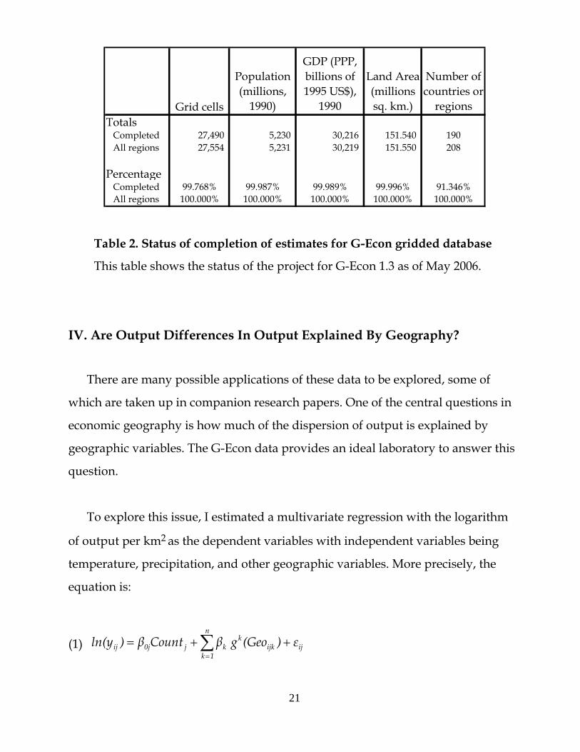
summary of the status of the data. Table 2 shows estimates for GEcon 1.3, which
was completed in May 2006. This table shows the number of grid cells, population,
output, land area, and number of countries or regions that have been completed.
The GEcon 1.3 database contains economic data on 190 completed countries
and regions, which comprise virtually all GDP, population, and terrestrial land
area. The only regions that are excluded are a few postage-stamp countries like
Mayotte and Liechtenstein.
Grid cells
Population (millions,
1990)
GDP (PPP, billions of 1995 US$),
1990
Land Area (millions sq. km.)
Number of countries or
regionsTotals Completed 27,490 5,230 30,216 151.540 190 All regions 27,554 5,231 30,219 151.550 208
Percentage Completed 99.768% 99.987% 99.989% 99.996% 91.346% All regions 100.000% 100.000% 100.000% 100.000% 100.000%
Table 2. Status of completion of estimates for G-Econ gridded database
This table shows the status of the project for G-Econ 1.3 as of May 2006.
IV. Are Output Differences In Output Explained By Geography?
There are many possible applications of these data to be explored, some of
which are taken up in companion research papers. One of the central questions in
economic geography is how much of the dispersion of output is explained by
geographic variables. The G-Econ data provides an ideal laboratory to answer this
question.
To explore this issue, I estimated a multivariate regression with the logarithm
of output per km2 as the dependent variables with independent variables being
temperature, precipitation, and other geographic variables. More precisely, the
equation is:
(1) ij
n
1kijk
kkj0jij ε)(GeogβCountβ)ln(y + += ∑
=
21
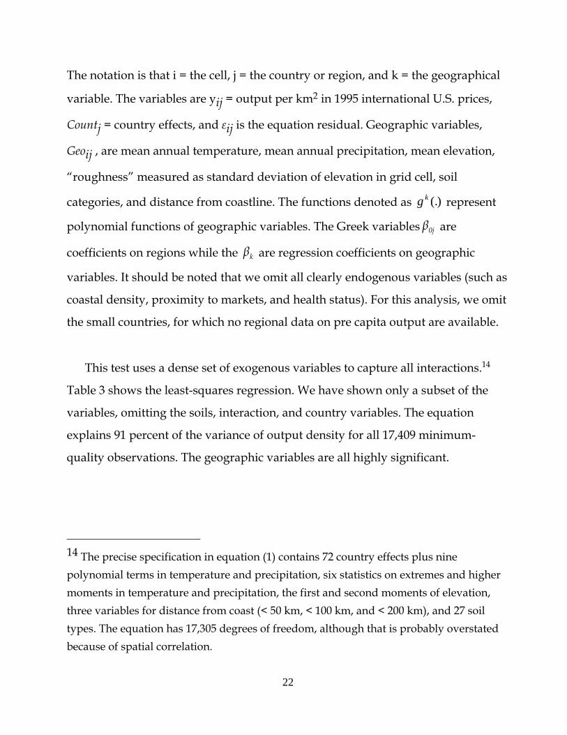
The notation is that i = the cell, j = the country or region, and k = the geographical
variable. The variables are yij = output per km2 in 1995 international U.S. prices,
Countj = country effects, and εij is the equation residual. Geographic variables,
Geoij , are mean annual temperature, mean annual precipitation, mean elevation,
“roughness” measured as standard deviation of elevation in grid cell, soil
categories, and distance from coastline. The functions denoted as represent
polynomial functions of geographic variables. The Greek variables are
coefficients on regions while the
)(.kg
0jβ
kβ are regression coefficients on geographic
variables. It should be noted that we omit all clearly endogenous variables (such as
coastal density, proximity to markets, and health status). For this analysis, we omit
the small countries, for which no regional data on pre capita output are available.
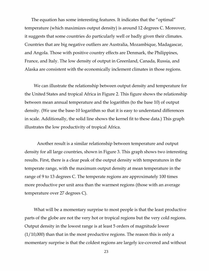
This test uses a dense set of exogenous variables to capture all interactions.14
Table 3 shows the least-squares regression. We have shown only a subset of the
variables, omitting the soils, interaction, and country variables. The equation
explains 91 percent of the variance of output density for all 17,409 minimum-
quality observations. The geographic variables are all highly significant.
14 The precise specification in equation (1) contains 72 country effects plus nine polynomial terms in temperature and precipitation, six statistics on extremes and higher moments in temperature and precipitation, the first and second moments of elevation, three variables for distance from coast (< 50 km, < 100 km, and < 200 km), and 27 soil types. The equation has 17,305 degrees of freedom, although that is probably overstated because of spatial correlation.
22
23
The equation has some interesting features. It indicates that the “optimal”
temperature (which maximizes output density) is around 12 degrees C. Moreover,
it suggests that some countries do particularly well or badly given their climates.
Countries that are big negative outliers are Australia, Mozambique, Madagascar,
and Angola. Those with positive country effects are Denmark, the Philippines,
France, and Italy. The low density of output in Greenland, Canada, Russia, and
Alaska are consistent with the economically inclement climates in those regions.
We can illustrate the relationship between output density and temperature for
the United States and tropical Africa in Figure 2. This figure shows the relationship
between mean annual temperature and the logarithm (to the base 10) of output
density. (We use the base-10 logarithm so that it is easy to understand differences
in scale. Additionally, the solid line shows the kernel fit to these data.) This graph
illustrates the low productivity of tropical Africa.
Another result is a similar relationship between temperature and output
density for all large countries, shown in Figure 3. This graph shows two interesting
results. First, there is a clear peak of the output density with temperatures in the
temperate range, with the maximum output density at mean temperature in the
range of 9 to 13 degrees C. The temperate regions are approximately 100 times
more productive per unit area than the warmest regions (those with an average
temperature over 27 degrees C).
What will be a momentary surprise to most people is that the least productive
parts of the globe are not the very hot or tropical regions but the very cold regions.
Output density in the lowest range is at least 5 orders of magnitude lower
(1/10,000) than that in the most productive regions. The reason this is only a
momentary surprise is that the coldest regions are largely ice-covered and without

24
human habitation or major economic activity (aside from isolated oil fields). The
true economic deserts of the globe are in Greenland, Antarctica, northern Canada,
Alaska, and Siberia.
V. Conclusion
This concludes the description of the G-Econ database for gridded output.
More detail on individual countries will be available on the project web site at
gecon.yale.edu. It must be emphasized that the current results are the first word and
not the last. If this approach to measuring economic activity proves fruitful, then
other researchers, particularly those in the countries involved, and especially
national statistical agencies, will be able to provide much more detailed and
accurate assessments of regional and gridded data, as well as time series. The
history of innovative data systems usually involves small-scale efforts by private
researchers to provide an example of how a particular data system might be
constructed or used. After the initial experience, if in fact the data set appears
valuable, more extensive and regular collection can be routinized and
institutionalized within government statistical agencies. 15 The production of
gridded global and national economic data by statistics agencies of governments is
entirely feasible once the general principles are developed, and it could form part
of the regular data collection and processing activities of governments.
15 For example, the U.S. national income and product accounts were first developed by a private researcher, Simon Kuznets, and were then lodged inside the government during the Great Depression when their value for understanding business cycles became clear. Similarly, after initial efforts to develop environmental accounts by private researchers, governments began to develop these accounts.

25
Dependent Variable: ln(output density)
Included observations: 17409
Weighting series: AREA
Variable Coefficient Std. Error t-Statistic Prob.
Mean Temp 0.511515 0.031529 16.22353 0.0000
Mean temp2 -0.009161 0.000307 -29.87665 0.0000
Mean temp3 -9.25E-05 1.03E-05 -8.936777 0.0000
Mean precip 0.010669 0.001134 9.407875 0.0000
Mean precip 2 -0.000237 1.12E-05 -21.14637 0.0000
Mean precip 3 4.91E-07 1.94E-08 25.36917 0.0000
Maximum temp -0.048580 0.040842 -1.189474 0.2343
Minimum temp -0.225336 0.035560 -6.336753 0.0000
Mean elevation 0.267036 0.037535 7.114287 0.0000
Coast distance: med 0.545384 0.067147 8.122203 0.0000
Coast distance: short 0.462837 0.075421 6.136724 0.0000
Coast distance: long 0.941525 0.050107 18.79012 0.0000
[other variables are
omitted
Weighted Statistics
R-squared 0.908350 Mean dependent var 9.135930
Adjusted R-squared 0.907730 S.D. dependent var 6.488201
S.E. of regression 1.970851 Sum squared resid 67162.64
Log likelihood -36454.51 F-statistic 326.0882
Durbin-Watson stat 0.607693 Prob(F-statistic) 0.000000
Table 3. Regression of ln of output density on geographic variables

0
1
2
3
4
5
6
7
8
9
-20 -10 0 10 20 30 40
Mean temperature
US observationsTropical African observations
Kernel fit, AfricaKernel fit, US
log
10 (o
utpu
t den
sity
, $ p
er k
m s
q)
Figure 2. Mean Temperature and ln Output Density for United States and
Tropical Africa.
Output measured as output per km2 for 1990, in 1995 U.S. dollars, purchasing
power parity. Solid lines are kernel fits to data for regions. Temperature is monthly
average Centigrade.
26

0
2
4
6
8
10
12
-40 -30 -20 -10 0 10 20 30 40
Mean temperature (C)
log1
0(ou
tput
den
sity
)
Figure 2. Kernel fit of average temperature and output density by grid cell
Output measured as output per km2 for 1990, in 1995 U.S. dollars, purchasing
power parity. Solid line is kernel fit. This shows results for all terrestrial grid cells
for which data are available (N = 19,919). Zero output is set at output per unit area
= 1.
27

28
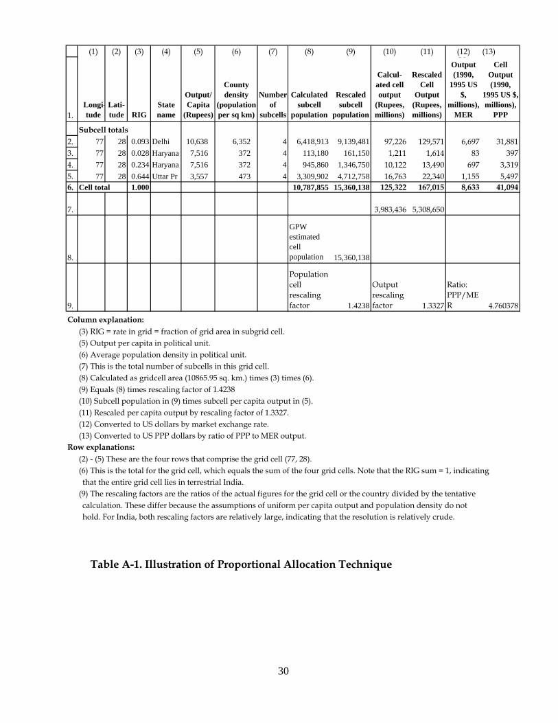
Appendix. Example of Application
of the Proportional Allocation Technique
This appendix shows the actual application of the technique to a single grid
cell in India. The data apply to the year 1990. Table A-1 shows the actual data for
the grid cell in which Delhi is located. Our convention is to label grid cells by the
coordinates at the southwest corner, so a coordinate of (latitude, longitude)
= (28, 77) indicates the grid cell centered at (28.5, 77.5). Southern and western
hemispheres are indicated by negative values. Also note that we use World Bank
national totals as controls for 1990, although that does not affect the algorithm
described here.
There are four sub-grid cells. The first step is to estimate the population of
each sub-grid cell. This is done by taking the area of each sub-grid cell and
multiplying it by the population density of the administrative unit. Summing over
the sub-grid cells gives a calculated grid cell population, here totaling 10.8 million.
However, the GPW estimate of grid cell population is 15.4 million, so the sub-grid
cell estimates are rescaled by a population rescaling factor (specific to each grid
cell), here equal to 1.42, to obtain the rescaled sub-grid cell population estimates
that are consistent with the GPW grid cell total.
The next step is to estimate the output of each sub-grid cell. These take the
rescaled population estimate for each sub-grid cell from column (9) and multiply
these by the per capita output of each administrative unit in column (5). (Note that
the per capita outputs of the administrative units are different.) The preliminary
calculation of gross cell product in row (6) of column (10) is derived by summing
the sub-grid cell estimates of output. This calculation provides an estimate of gross
cell product for grid cell (28, 77) of 125.3 billion rupees. An estimate of the gross

29
domestic product of India summing over calculated cell outputs for all sub-grid
cells (not shown) yields an estimate of total GDP that is lower than the control total
from the national accounts, so the sub-grid cell estimates are rescaled upwards
uniformly by the output rescaling factor of 1.3327.
The final estimate of the gross cell output is then 167.0 billion rupees, shown
in row (6) of column (11). We then convert this number into U.S. dollars at market
exchange rates by multiplying by an exchange rate of 19.3 rupees per dollar. These
are also converted into a PPP level of output by multiplying the MER number by a
conversion rate of 4.76 PPP units of output per MER unit of output.
The final results for grid cell (77, 28), in local currency, U.S. dollars at MER,
and U.S. dollars at PPP, are shown in columns (11) through (13) of row (6).
(1) (2) (3) (4) (5) (6) (7) (8) (9) (10) (11) (12) (13)
1.Longi-tude
Lati-tude RIG
State name
Output/ Capita
(Rupees)
County density
(population per sq km)
Number of
subcells
Calculated subcell
population
Rescaled subcell
population
Calcul-ated cell output
(Rupees, millions)
Rescaled Cell
Output (Rupees, millions)
CeOutput (1990,
1995 US $,
millions), MER
Cell Output (1990,
1995 US $, millions),
PPP
Subcell totals2. 77 28 0.093 Delhi 10,638 6,352 4 6,418,913 9,139,481 97,226 129,571 6,697 31,8813. 77 28 0.028 Haryana 7,516 372 4 113,180 161,150 1,211 1,614 83 3974. 77 28 0.234 Haryana 7,516 372 4 945,860 1,346,750 10,122 13,490 697 3,3195. 77 28 0.644 Uttar Pr 3,557 473 4 3,309,902 4,712,758 16,763 22,340 1,155 5,4976. Cell total 1.000 10,787,855 15,360,138 125,322 167,015 8,633 41,094
7. 3,983,436 5,308,650
8.
GPW estimated cell population 15,360,138
9.
Population cell rescaling factor 1.4238
Output rescaling factor 1.3327
Ratio: PPP/MER 4.760378
Column explanation:(3) RIG = rate in grid = fraction of grid area in subgrid cell.(5) Output per capita in political unit.(6) Average population density in political unit.(7) This is the total number of subcells in this grid cell.(8) Calculated as gridcell area (10865.95 sq. km.) times (3) times (6).(9) Equals (8) times rescaling factor of 1.4238(10) Subcell population in (9) times subcell per capita output in (5).(11) Rescaled per capita output by rescaling factor of 1.3327.(12) Converted to US dollars by market exchange rate.(13) Converted to US PPP dollars by ratio of PPP to MER output.
Row explanations:(2) - (5) These are the four rows that comprise the grid cell (77, 28). (6) This is the total for the grid cell, which equals the sum of the four grid cells. Note that the RIG sum = 1, indicatingthat the entire grid cell lies in terrestrial India.
(9) The rescaling factors are the ratios of the actual figures for the grid cell or the country divided by the tentativecalculation. These differ because the assumptions of uniform per capita output and population density do nothold. For India, both rescaling factors are relatively large, indicating that the resolution is relatively crude.
Table A-1. Illustration of Proportional Allocation Technique
30


