The Impact of Consumer Inattention on Insurer Pricing in the
Medicare Part D Program∗
Kate Ho† Joseph Hogan ‡ Fiona Scott Morton §
February 8, 2017
Abstract
Medicare Part D presents a novel privatized structure for a government pharmaceutical
benefit. Incentives for firms to provide low prices and high quality are generated by consumers
who choose among multiple insurance plans in each market. To date the literature has primarily
focused on consumers, and has calculated how much could be saved if choice frictions were
removed. In this paper we take the next analytical step and consider how plans would adjust
prices if consumer search behavior improved and consumers became more elastic. Margins
should fall, leading to additional consumer and government savings. We estimate a model of
consumer plan choice with inattentive consumers. We then turn to the supply side and examine
insurer responses to this behavior. We show that high observed premiums are consistent with
insurers profiting from consumer inertia. We use the demand parameters and a simple model
of firm pricing to approximate how much lower steady state Part D plan premiums would be
if consumers were attentive. Our estimates indicate that an average consumer could save over
$1000 over three years when firms’ lower markups are taken into account. Further, since the
government pays three-quarters of the cost of the Part D program, government expenditures
would also fall. Our simulations indicate the government could save $1.3 billion over three years,
or 1% of the cost of subsidizing the relevant enrollees.
∗We thank Mark Duggan, Liran Einav, Gautam Gowrisankaran, Ben Handel, Robin Lee, Bentley MacLeod, AvivNevo, Eric Johnson and participants at the NBER I.O. Summer Institute for helpful comments. We especially thankFrancesco Decarolis for sharing his data with us. All errors are our own.†Columbia University and NBER, [email protected].‡Columbia University, [email protected].§Yale University and NBER, [email protected].
1

1 Introduction and Motivation
The addition of pharmaceutical benefits to Medicare in 2006 was the largest expansion to
the Medicare program since its inception. Not only is the program large, it is also innovative in
design. Traditional Medicare Parts A and B are organized as a single-payer system; enrollees see
the physician or hospital of their choice and Medicare pays a pre-set fee to that provider, leaving no
role for an insurer. In contrast, Part D benefits are provided by private insurance companies that
receive a subsidy from the government as well as payments from their enrollees. The legislation
creates competition among plans for the business of enrollees, which is intended to drive drug prices
and premiums to competitive levels. Each Medicare recipient can choose among the plans offered
in her area based on monthly premiums, deductibles, plan formularies, out-of-pocket costs (OOP
costs or copayments) for drugs, and other factors such as the brand of the insurer and the quality
of customer service.
The premise of the Part D program was that consumers’ ability to choose their preferred plan
would discipline insurers into providing lower prices and higher quality than would be achieved
through a government-run plan. Critically, these better outcomes require that consumers choose
effectively, so that demand shifts to plans that consumers prefer because they offer low prices or
high quality. If consumers choose plans randomly, a plan will have no incentive to lower its price
since this will not affect enrollment, and markups will be high. In contrast, if many consumers
choose to enroll in a plan that lowers its price, markups will fall as firms offer lower premiums to
consumers.
This paper analyzes the supply-side response to imperfect consumer demand in Part D. We
demonstrate that, in reality, consumer choices are made with substantial frictions. Consumers
rarely switch between plans and do not consistently shop for price and quality when they do switch,
reducing the effective demand elasticity faced by insurers. We provide evidence that, because of
the absence of strong disciplining pressures from consumers, insurers set prices above the efficient
level. Thus plans extract high rents due to consumer inattention. Not only would improved con-
sumer search benefit consumers directly, it would also lead to plan re-pricing that would save both
consumers and the government significant sums. Our estimates indicate that removing inattention
and allowing prices to adjust while leaving other sources of consumer preferences unchanged could
reduce consumer expenditures by over $1000 per enrollee over the three years 2007-9. Under our
assumptions, government program costs would fall by $1.3 billion over the same period due to plan
re-pricing. To our knowledge, this is the first paper to estimate the impact of reduced consumer
inertia through both demand and supply-side channels. We find that the insurer response - lowering
premiums - results in significant savings to both enrollees and taxpayers.
One concern when Part D began was that the prices the plans paid for drugs would rise because
plans would lack the bargaining power of the government. Duggan and Scott Morton (2010)
demonstrate that this did not happen. Rather, prices for treatments bought by the uninsured elderly
fell by 20% when they joined Part D. Since the program’s inception, increases in pharmaceutical
prices have been restrained. This is due in part to aggressive use of generics by many insurers, but
2

also to insurers’ ability to bargain for rebates in exchange for favorable formulary placement and
therefore market share. According to Congressional Budget Office estimates, drug costs under the
basic Part D benefit increased by only 1.8% per beneficiary from 2007-2010 net of rebates. The
remainder of plan expenditures - approximately 20% of total costs according to the CBO - consists
of administration, marketing, customer service, and like activities. The PCE deflator for services
during this same time period increased at an average annual rate of 2.40%. Yet, despite these
modest increases in the costs of providing a Part D plan, premiums in our data were on average
62.8% higher in 2009 than they were in 2006, the first year of the program, which corresponds
to a 17.6% compound annual growth rate. The CBO estimates indicate that plan profits and
administrative expenses per beneficiary (combined) grew at an average rage of 8.6% per year from
2007 to 2010.
These figures raise the question of why slow growth in the costs of drugs and plan administration
were not passed back to consumers in the form of lower premiums. One possibility is that Part
D may be well designed to create competition among treatments that keeps the prices of drugs
low, yet may not do so well at creating competition among plans in order to restrain the prices
consumers face. Since the program is 75% subsidized by the federal government, any lack of effective
competition would increase government expenditures as well as consumer costs. Our objective in
this paper is to investigate the extent to which consumer choice imperfections in this market impede
competition between plans.
Part 2 of the paper describes the Medicare Part D program and discusses reasons for search
imperfections. In Parts 3 and 4 we review the literature related to consumer demand with choice
frictions, in Medicare Part D and elsewhere, and the dynamics of pricing in that environment. In
Part 5 we describe our dataset, which provides detailed information on the choices and claims of non-
subsidized enrollees in New Jersey. In Part 6 we observe that consumers consistently make choices
that are financially costly given their consumption patterns, and that this pattern of choosing
expensive plans when cheaper ones are available does not appear to diminish with either experience
in the program or time. Consumers seem to switch plans in response to “shocks” to their health
or current plan characteristics, but are much less sensitive to changes in other plans. Motivated
by these findings, we develop a two-stage consumer decision model for estimation which accounts
for inattention as a source of inertia. We identify the effect of consumer inattention separately
from other potential sources of choice persistence, such as persistent heterogeneous unobserved
preferences, using a detailed panel dataset which documents the choices of new entrants to the
Part D program and then follows each individual’s choices over time. Our identification strategy
is similar to that utilized in recent related papers that investigate the reasons for consumer choice
persistence in other health insurance programs (Handel (2013), Polyakova (2014)). The estimates
indicate that inattention is an important part of the story.
Having established the behavior of consumers, we turn to analysis of the supply side of the Part
D marketplace in Section 7. Using a dataset of nationwide plan characteristics and enrollment,
we show that plans with larger market shares set prices in a manner consistent with high choice
3
frictions. We also document rapid growth in plan prices that is not accounted for by changes in
costs, and high dispersion in relatively homogenous standard benefit plans that is indicative of
search frictions.
The final section of the paper, Section 8, uses the estimated demand model to conduct simula-
tions that allow the supply side to adjust to a reduction in the proportion of consumers who are
inattentive. We focus on plan premium choices. We abstract away from dynamics and model plans
as profit-maximizing insurers that take into account the elasticity of demand, including consumers’
attentiveness, when choosing a markup over cost. More attentive and price-elastic consumers will
generate lower insurer margins. We use accounting data from the Part D program to estimate firm
costs and then predict plans’ optimal static premium bids under various assumptions regarding the
proportion of consumers who are inattentive, and hence the expected premium sensitivity faced by
insurers. We show that the greater the percent inattentive, the higher the optimal premium bids
chosen by plans. In our preferred simulation, removing inattention—and allowing plans to reprice
in response to this change—would generate savings of $1,050 per consumer over the years 2007-
2009. These results indicate that even if consumers do not choose the lowest-cost plan for them,
whether due to information processing costs or for other reasons, simply prompting them to choose
a new plan every year has a substantial effect on costs through the channel of plan premiums. If
we assume these changes can be generalized to plans nationwide, the federal government would
save $1.3 billion between 2007-2009 if inattention was removed. While we note that allowing for
dynamic pricing would affect these predictions, perhaps generating an increase in premiums over
time as plans “invest” to attract enrollees and then “harvest” their installed base, our static anal-
yses are sufficient to demonstrate the substantial long-run savings, to consumers and government,
that could result from increasing competition through reduced inattention.
Studies such as ours are crucial both to future policies concerning Part D plan design, infor-
mation provision, and quality regulation, but also to those same issues in health insurance. The
Patient Protection and Affordable Care Act (2010) created health plan exchanges through which
consumers who are not eligible for employer-sponsored insurance can access health insurance cov-
erage. In this setting consumers again face an array of plans, regulated in quality, and provided by
private insurers. The use of competition as a means to control costs and deliver quality requires
policy-makers to make choices regarding the design and regulation of such marketplaces.
2 Medicare Part D
Pharmaceutical benefits were not part of Medicare when it was first launched in 1965. However,
the rising share of pharmaceuticals in the cost of healthcare created significant OOP expenditures
for seniors and led to the creation of the Part D program under President Bush in 2006. The
novelty of this government benefit is the fact that it is essentially privatized: insurance companies
and other sponsors compete to offer subsidized plans to enrollees. The sponsor is responsible for
procuring the pharmaceutical treatments and administering the plan.
4
The Basic Part D plan is tightly regulated in its benefit levels so that there is limited flexibility
for plans to reduce quality and thereby lower costs and attract enrollees. Plans must offer coverage
at the standard benefit level, and each bid must be approved by the Centers for Medicare and Med-
icaid Services (CMS). The coverage rules include restrictions on plans’ formularies, including which
therapeutic categories or treatments must be covered. Plans are mandated to cover “all or substan-
tially all” drugs within six “protected” drug treatment classes, as well as two or more drugs within
roughly 150 smaller key formulary types. The protected classes include many treatments that would
identify very sick patients such as AIDS drugs, chemotherapy treatments, and antipsychotropics.
Plans’ placement of these drugs on their formulary is required, and the cost-sharing required of
beneficiaries is carefully scrutinized by CMS to ensure plans are not discriminating against sick
beneficiaries. Hence it is not straightforward for a plan to avoid the sickest enrollees; this was
particularly true in the first years of the program when it was unclear which enrollees would have
particular costs or utilization profiles and there was no usage history. Moreover, subsidy payments
to plans are risk-adjusted according to their enrollee’s demographics and health status. There is
an additional multiplier to increase the subsidy for low-income and institutionalized status. Thus
sponsors receive higher payments for sicker enrollees which reduces their incentive to seek out
healthy participants. In addition, plans must evaluate their predicted costs using CMS-specific
actuarial models. This limits their ability to attract consumers by shifting costs to a part of the
benefit that the enrollee has difficulty evaluating or will pay later. The result of this fairly tight
regulatory environment is that the plan’s premium emerges as its most salient characteristic for
consumers, particularly for the defined standard benefit plan.1 We will see in our empirical work
that consumers place high weight on a plan’s premium when they make choices among plans. The
deductible and other characteristics have an effect, but their empirical magnitude is much smaller
than that of the premium.
Enrolling in Part D is voluntary, and one might be concerned that adverse selection would mean
only sick seniors enroll. However, the subsidy for the program is set by legislation to be an average
of 74.5% of costs, so for the vast majority of seniors, enrolling is financially favorable (see Heiss et
al. (2006)) and most eligible seniors did enroll. In addition, the newly eligible who delay enrolling
(perhaps until they become sick) are required to pay a higher price for coverage when they do join.
Many observers have noted that the Part D choice problem is difficult and the empirical liter-
ature indicates that consumers do not choose plans that minimize their costs. In 2006 when the
program began there were at least 27 plans offered in each county in the US. Enrollees had to con-
sider how premiums varied across these plans, forecast their drug consumption in the year ahead
and compare the OOP costs for that set of drugs across plans. In addition enrollees might receive
an adverse health shock during the year that would change the set of medications demanded, ne-
cessitating the comparison of expected expenditures across plans. Furthermore, no major program
like this existed in the US at the time Part D began, so seniors likely had no experience attempting
1As we show in the paper, enrollees can do better by searching for the plan-specific out-of-pocket payments forthe particular drugs they will consume.
5
to make these calculations. Lastly, most Part D consumers are older Americans; outside the dual-
eligible and disabled, Medicare eligibility begins at age 65. Finding a low-cost plan in the Part D
program therefore requires the elderly to carry out a fairly difficult cognitive task.
Part D benefits are provided through two types of private insurance plans. The first is a simple
prescription drug plan (PDP) which provides coverage only for prescription drug costs for seniors
enrolled in the standard fee-for-service Medicare program (which does not cover drug costs). In
2006, 10.4 million people enrolled in PDPs. Medicare Advantage plans (MA-PD), for seniors who
have opted out of standard Medicare, function similarly to an HMO; such plans insure all Medicare-
covered services, including hospital care and physician services as well as prescription drugs. In
2006, 5.5 million people enrolled in MA-PDs. By 2013, of the 32 million Part D enrollees, almost 20
million were enrolled in PDPs. MA-PD plans have particularly low enrollment in New Jersey, the
state from which our data are taken: only 18-20% of NJ Part D enrollees were in MA-PD plans in
2006-9, compared to 32-38% in the U.S. overall. This paper focuses solely on PDPs and prescription
drug coverage. We assume that PDP enrollees do not consider enrolling in an MA-PD plan. We
justify this assumption by noting both the low share of New Jersey MA-PD plans and the fact that
moving from a stand-alone PDP to an MA-PD plan incurs the substantial cost of changing coverage
(and potentially providers) for hospital and physician services as well as prescription drugs.
A fee-for-service Medicare enrollee can choose among all the PDPs offered in her region of the
country. A plan sponsor contracts with CMS to offer a plan in one (or more) of the 34 defined
regions of the US. The actuarial value of the benefits offered by a plan must be at least as generous
as those specified in the legislation. In the 2006 calendar year this included a deductible of $250, a
25% co-insurance rate for the next $2000 in spending, no coverage for the next $2850 (the “coverage
gap”), and a five percent co-insurance rate in the “catastrophic region”, when OOP expenditures
exceed $3600. As these figures change annually, we report them through 2013 in Appendix Table
A1. A sponsor may offer a basic plan with exactly this structure, or one that is actuarially equivalent
- for example with no deductible but higher cost-sharing. Enhanced plans have additional coverage
beyond these levels and therefore higher expected costs and higher premiums.2
The way in which sponsors bid to participate in the program is important to an analysis of
competition. Sponsors must apply to CMS with a bid at which each plan they wish to offer will
provide the benefits of a basic plan to enrollees.3 Importantly, the costs that the plan is meant to
include in its bid are those it will expend to administer the plan, including for example, the cost
of drugs, overhead, and profit, and net of any costs paid by the enrollee such as the deductible or
copayments and reinsurance paid by CMS.4 The bid is supposed to reflect the applicant’s estimate
2The added benefit typically takes the form of either additional coverage in the coverage gap, reduced copayments,or coverage of certain drug types excluded from normal Part D coverage, such as cosmetic drugs and barbiturates.Plan sponsors offering plans with enhanced coverage must also offer a basic plan within the same region, and sponsorsare prohibited from offering more than two enhanced plans in a given region. Enhanced plans do not receive highersubsidies, and any incremental costs are paid entirely by enrollees.
3Any costs of enhanced benefits in enhanced plans must be excluded at this stage.4CMS may not bargain with plans over their bids. The agency may disallow a bid if some aspect of the plan such
as the formulary or the actuarial equivalence does not follow regulations.
6

of its “average monthly revenue requirements” (i.e. how much it wants to be paid) to provide
basic Part D benefits for a well-defined statistical person. CMS takes these bids and computes a
“national average monthly bid amount” (NAMBA).5 CMS uses the government subsidy percentage
(74.5%) plus an estimate of its reinsurance costs and other payments to determine how much of
the bid the beneficiaries must pay on average. This is called the beneficiary premium percentage,
and in the first year of the program it was 34%6. The Base Beneficiary Premium (BBP) is then
the average bid (NAMBA) times the percentage payable by consumers. The premium for any
given plan is this BBP adjusted by the full difference between the plan’s own bid and the NAMBA
average. If a plan’s monthly bid is $30 above NAMBA, then its premium will be $30 above the
BBP, and similarly if the bid is below the NAMBA (with the caveat that the premium is truncated
at zero). This scheme makes the consumer bear higher premiums at the margin, which contributes
to differences in premiums being important in consumer choice.
Two types of beneficiaries do not pay the full cost of Part D coverage. Approximately 6.3
million dual-eligible Medicaid recipients were automatically enrolled in Part D in 2006, as were
an additional 2.2 million Low Income Subsidy (LIS) recipients. Premiums and OOP costs are
fully paid by the government for the former, while the latter receive steep discounts. Foreseeing
that LIS enrollees might be less price sensitive than regular enrollees, the Part D regulations only
provide a full subsidy for LIS recipients who choose a plan with costs below the benchmark for
their region.7 If a plan loses benchmark status, its enrollees are automatically reassigned (equally
across qualifying plans) to a benchmark plan in their region unless they choose to opt out and pay
the cost difference themselves. Approximately 10% of enrollees in this category chose to opt out
and become active “choosers” in 2007-8 (Summer et al 2010). While our demand model considers
only non-LIS enrollees who are not dual eligible, that paper suggests that LIS enrollees who opted
out behaved in a manner consistent with inattention, like the population we consider.8
The participation of private sector insurers in this new program in 2006 was voluntary and
therefore uncertain. However, it turned out that many sponsors, both public and private, entered
the Part D market in 2006. There were 1429 PDP plans offered nationwide in 2006 (though this
had fallen to 1031 by 2013); every state had at least 27 PDPs every year during our sample period.
Enrollees select one of these plans during the open enrollment period each November to take effect
5In 2006 the various plans were equally weighted, but from 2008 onwards the NAMBA slowly transitioned to anenrollment weighted average.
6The sum of the government subsidy and the beneficiary premium percentage is over 100% because part of thegovernment subsidy is used for plan reinsurance rather than as a direct subsidy to premiums.
7For the first three years of the program, the benchmark was calculated as the equal-weighted mean basic PDPplan premium in a region. In later years it was an enrollment-weighted mean. Since lower cost plans have moreenrollees, this policy change reduced the number of plans that qualified as benchmark over time.
8Since carriers set a single premium for a plan that enrolls both LIS and non-LIS consumers, there may beinteractions between the two markets. For example, a strategy studied by Decarolis (2012) in the early years of PartD involved cycling of plans. A sponsor would raise the price of an existing plan above the benchmark, but introducea new plan below the benchmark to catch auto-assigned LIS recipients, meanwhile keeping any choosers and otherenrollees in the original plan. We note that this cycling strategy was not used by all insurers, and declined over time.For example, Summer et al (2010) report that by 2010, 92% of all auto-assignments were across corporate boundaries.In the analysis below we find no evidence of this cycling behavior by plans in our New Jersey sample; we do notattempt to account for it in our model of supply.
7

in the subsequent calendar year. The program includes many sources of aid for enrollees in making
these decisions. Most importantly, CMS has created a website called “Planfinder” that allows a
person to enter her zip code and any medications and see the plans in her area ranked according
to OOP costs. The website also enables prospective enrollees to estimate costs in each plan under
three health statuses (Poor/Good/Excellent), to estimate costs in standard benefit plans based
on total expenditures in the previous year, and to filter plans based on premiums, deductibles,
quality ratings and brand names. A Medicare help line connects the enrollee to a person who
can use the Planfinder website on behalf of the caller in order to locate a good choice. However,
conversations with CMS representatives suggest that very few enrollees make full use of the website.
Pharmacies, community service centers, and other advocates offer advice. Survey evidence (Kaiser
Family Foundation (2006), Greenwald and West (2007)) indicates that enrollees rely on friends and
family to help them choose a Part D plan, yet still find the choice process difficult.
3 Literature Review: Consumer Demand
The introduction of Part D immediately created a literature evaluating outcomes from the
novel program structure. An important early paper documenting that the elderly do not choose
optimally is that of Abaluck and Gruber (2011, hereafter AG). Using a subset of claims data from
2005 and 2006 and a similar methodology to our own, the authors show that only 12% of consumers
choose the lowest cost plan; on average, consumers in their sample could save 30% of their Part
D expenditure by switching to the cheapest plan. Consumers place a greater weight on premium
than expected OOP costs, don’t value risk reduction, and value certain plan characteristics well
beyond the way those characteristics influence their measure of expected costs. These results have
been largely corroborated by Heiss et al. (2013) and Ketcham et al. (2012) among others.
Other studies have examined infrequent switching between plans as an explanation for inefficient
consumer choice in the Part D market. In a field experiment, Kling et al. (2012) show that
giving Part D consumers individualized information about which plans will generate the most
cost savings for them can raise plan switching by 11% (from 17% to 28%) and move more people
into low-cost plans. Ketcham et al. (2015) use administrative data through 2010 to show that
switching increases when more plans are available and that people become more responsive to
large increases in their plans’ costs over time. Polyakova (2016) estimates a model of plan choice
featuring consumer switching costs and adverse selection, with unobservably riskier beneficiaries
choosing more comprehensive coverage. She uses the model to simulate the effect of closing of the
coverage gap on adverse selection and finds that switching costs inhibit the capacity of the regulation
to eliminate sorting on risk. The presence of switching costs and consumer choice frictions has been
documented in other health insurance markets by Handel (2013) among others.
Abaluck and Gruber followed up their results with a study of how enrollees’ choices varied
across the first four years of Part D (Abaluck and Gruber (2013), hereafter AG13). AG13 finds
that consumers continue to make significant mistakes and that there is no measurable learning
8
over time in their national sample. These findings are consistent with the estimates from our New
Jersey sample. In both sets of results consumers continue to be extremely sensitive to premiums.
The empirical specification in AG13 is more reduced form than our model, but the two papers
estimate similar levels of welfare loss from inertia. AG13 controls for brand fixed effects but still
finds a strong role for inertia, concluding “rather than reflecting persistent unobserved factors of
chosen plans, [inertia] reflect[s] either adjustment costs or inattention.” Our paper explores the
inattention hypothesis in more detail. Our specification separately models consumer inattention,
consumer valuation of the insurer’s brand, and also persistent unobserved heterogeneity in prefer-
ences for a particular product. We continue to find an empirical role for inattention even in this
more sophisticated choice environment. AG13 concludes that choice inconsistencies are “driven
by changes on the supply side that are not offset both because of inertia and because non-inertial
consumers still make inconsistent choices.” By modeling the supply side, as we do in this paper,
we can simulate how insurers will set premiums in response to changing consumer attention. This
step has received very little attention in the Part D literature. Ketcham, Kuminoff and Powers
(2016) predict the impact of various policies to reduce the impact of choice imperfections in Part
D, for example by reducing the size of the choice set, but they assume plan premium adjustments
are designed to maintain the net revenue per enrollee that they earned prior to the policy. This
assumption does not capture the impact of consumer inattention on plan markups that is the focus
of this paper.
There is a great deal of research in both psychology and economics literatures on consumer
search and choice. Iyengar and Kamenica (2010) provide evidence that more options result in
consumers making worse choices. In contrast to the prediction of a standard neoclassical model,
more choice may not improve consumer welfare if it confuses consumers and leads them to seek
simplicity. A large literature studies the importance of information processing costs to explain
deviations from the choices expected of computationally unconstrained agents (see Sims (2003)
and Reis (2006) for examples). Models of consumer search with learning, where each consumer
uses the observed price of a single product to infer the prices likely to be set by other firms, also
indicate that consumers may incur excessive costs by searching either too little or too much (e.g.
Cabral and Fishman (2012)). Agarwal et al.(2009) show that the ability to make sound financial
decisions declines with age. Since Part D enrollees are either disabled or elderly, and seem likely to
experience cognitive costs of processing information, it may be reasonable to expect less optimal
behavior from Part D consumers than from the population as a whole. These types of results
have led some critics of Part D to call for CMS to limit the number of plans available to seniors.
On the other hand, using data on private-sector health insurance, Dafny et al. (2013) show that
most employers offer very few choices to their employees and that employees would greatly value
additional options. Moreover the results from Stocking et al. (2014) suggest that merely limiting
the number of available plans would not be sufficient, as this would limit competition and lead to
higher prices. Thus while the difficulty of choosing an insurance plan may lead consumers to choose
expensive plans, it is not clear that limiting the range of options is the correct policy response.
9
Other authors have found evidence for inattention or lack of comparison shopping in complex
and infrequent purchase decisions. In the auto insurance market, Honka (2014) finds that consumers
face substantial switching costs, leading them to change plans infrequently, and that search costs
lead those who switch to collect quotes from a relatively small number of insurers. Sallee (2014)
uses the idea of rational inattention to explain why consumers under-weight energy efficiency when
purchasing durable goods. Busse et al. (2010) find that consumers are inattentive and use a limited
number of “cues” such as price promotions and mileage thresholds to evaluate auto purchases rather
than actual prices and qualities. Luco (2016) and Illanes (2016) consider switching costs and firm
competition in retirement investment choices. Hortacsu et al (2015) examine consumer choices
and switching behavior among retail electricity suppliers in Texas and conclude that high search
frictions lead to a high market share for the incumbent supplier.
4 Dynamics and Pricing Responses
Farrell and Klemperer (2007) surveys the substantial theoretical literature considering the
effects of consumer switching costs and other sources of inertia on firm competition and pricing.
There are two sets of results: the first relates to price changes over time while the second considers
steady state price levels. We discuss both here but focus on the latter in our estimation.
Papers such as Klemperer (1987) and Klemperer (1995) argue that, if firms cannot commit
to future prices, consumer switching costs provide an incentive to “invest” and then “harvest”.
“Investing” is the process of building up market share through low prices in order to increase
future profits, while “harvesting” is the process of reaping those profits by raising prices on an
installed base. If the market begins in some particular period (as in 2006 for Medicare Part D),
and all consumers have zero switching costs in that period, one might expect to see low initial prices
and then price increases over time as the incentive to harvest the installed base increases relative to
the incentive to attract new market entrants. In the longer term, once the market reaches steady
state, multiple possible pricing patterns could emerge. If firms cannot discriminate between cohorts
of consumers (as in the Part D application), new firms may choose a single price that is attractive
to new consumers, and thereby effectively specialize in selling to new customers. Firms with old
locked-in customers will choose a single price that is higher, and effectively specialize in selling only
to old consumers, leading to cycling (Farrell and Klemperer 2007). Alternatively, a firm may hold a
“sale” in a particular period to attract new customers, while other firms pursue the same strategy
in possibly different periods (Farrell and Shapiro 1988, Padilla 1995).
Several prior empirical studies have investigated the evidence for these dynamic pricing patterns
in the presence of choice frictions. Ericson (2012) and Ericson (2014) analyze the insurer’s problem
in Medicare Part D and show that firms initially set relatively low prices for newly introduced plans,
but then raise prices as plans age, consistent with the “invest then harvest” dynamic. Similar
questions have been studied empirically in other markets, e.g. by Miller (2014) in the case of
Medicare Advantage, and Cebul et al (2011) in commercial health insurance. Decarolis (2015) and
10
Decarolis et al (2014) also study the supply side of the Part D market paying particular attention
to the interaction of low-income subsidy and other enrollees.
We show below that premium trends in the data are consistent with the predictions of these
models: premiums increase substantially between 2006-2009, and they increase particularly for the
plans with the greatest incentive to harvest their installed base (those with the greatest number of
enrollees and in years with the smallest number of new entrants aging into Part D). However we do
not explicitly model price dynamics and our counterfactual analyses do not predict price patterns
over time. Instead our simulations utilize the predictions of theoretical papers that analyze the
impact of switching costs on price levels.
Beggs and Klemperer (1992) examine a no-sale equilibrium of an infinite-period duopoly model
with consumer switching costs, in which in every period new consumers arrive and a fraction of old
consumers leaves. Firms cannot discriminate between these groups of consumers. Consumers are
forward-looking and firms make dynamic profit-maximizing pricing decisions. Under the assump-
tion that switching costs are sufficiently large that old consumers are locked into the product they
have previously bought, there is a steady state Markov perfect equilibrium where firm prices are
higher than in the model without switching costs.9 The intuition is that consumer lock-in gives the
firm effective market power over some portion of consumers, which implies a price increase relative
to the case with no switching costs. A similar intuition is provided in Radner (2003) which considers
a model of “viscous demand”, i.e. where demand adjusts slowly to changes in prices. This viscosity
provides the firm with a kind of market power since it can raise its price above that of competitors
without immediately losing all of its customers. In the homogenous product duopoly case there is a
family of Nash equilibria where, once firms have achieved their target market shares and the total
target market penetration, they both charge a price equal to consumers’ willingness to pay (similar
to a collusive outcome, with prices strictly greater than the equilibrium price without viscosity).
Farrell and Klemperer (2007) summarize these models, and other related papers, and conclude
that there is a “strong presumption” that switching costs make markets less competitive, i.e. lead
to increased equilibrium prices.10 Moreover, our setting has an additional feature that reinforces
this conclusion. We find that consumer inertia in the Part D setting is caused by inattention (or
asymmetric search costs) rather than switching costs of the conventional type. Since incumbent
enrollees in a particular plan will only rarely notice other plans’ prices, the incentive for firms to
reduce prices in order to attract consumers from competitors (“invest”) is small compared to a
9The authors note that the results will also hold if there is a startup cost K of trying a brand and K′ of switchingto a new brand, for K,K′ sufficiently large.
10Work such as Dube, Hitsch and Rossi (2008) shows that this result may not hold in cases where a firm’s incumbentcustomers are not fully locked into a single firm. That paper solves and/or simulates several simplified versions ofa model with differentiated products, consumer switching costs and imperfect lock-in. The authors show that asswitching costs grow, equilibrium prices first fall and then increase relative to the case with no switching costs. Theintuition is that with low switching costs the incentive for a firm to invest in future loyalty, and attract consumersfrom its competitors, by lowering current prices can dominate the incentive to harvest. The competitor anticipatesthis and lowers its price to prevent the customer from switching. This effect is much less relevant for our settingbecause inattention is unlike other switching costs. Inattentive consumers do not notice a lower price and thereforecannot be attracted by it.
11

model with conventional switching costs. The intuition in Beggs and Klemperer (1992) is therefore
likely to hold in the Part D context: equilibrium prices are likely to be higher than in the case
without consumer inattention.11
Our counterfactual analyses investigate the magnitude of the steady state price increases likely
to be generated by inattention given our estimated model. We abstract from firm dynamic choices.
We are interested in the steady state pricing of a marketplace of plans selling to fully attentive
consumers compared to one pricing to inattentive consumers. We argue, following the intuition
in Beggs and Klemperer (1992) and related papers, that the existence of inattentive enrollees
has the effect of reducing the average elasticity faced by insurers. The true elasticity of any
consumer’s demand does not change, but a fraction of consumers is inattentive and therefore
behaves inelastically. This group does not switch plans in response to a price increase and therefore
lowers the effective insurer elasticity of demand. We use this insight to generate a range of estimates
of the premium effect of inattention.
5 Data
Our primary data source, provided by the Centers for Medicare and Medicaid Services (CMS),
contains information on prescriptions and plan choices for Part D enrollees from New Jersey in
2006-9. Our data consist only of enrollees who did not have LIS status at any time and who were
enrolled in stand-alone PDPs, rather than MA plans. Limiting the study to these enrollees reduced
the population size from all New Jersey enrollees in PDP plans, of which there were between 527,000
and 545,000 from 2006 to 2009, to between 300,000 and 325,000 over the same time period. We
chose New Jersey partially because it had a very low percentage of MA-PD enrollees compared to
the national average—18-20% of NJ enrollees were in MA-PD plans compared to a national average
of 32-38%—and because the total number of enrollees that met our criteria was not far above the
CMS cutoff of 250,000. From this subpopulation we drew a random sample in 2006 and a random
sample of new enrollees in 2007-9 to bring the total sample up to 250,000 enrollees. We limited the
sample to unsubsidized PDP enrollees in order to focus on a setting where consumers had to pay
the listed price for every plan and where plans had relatively standardized quality (not the case for
MA-PD plans which include medical as well as pharmacy benefits). Details of the data cleaning
procedure are provided in Appendix A.
Appendix Table A2 shows the number of enrollees in our dataset each year, ranging from 127,000
in the first year of the program up to 160,000 in 2009. Just over 60% of enrollees are female, and
about 90% are white. The breakdown by age group is also shown in the table. Over our sample
period the entering cohort, ages 65-69, grows in size from under 20% to almost 28% of the sample.12
11The papers on consumer search and learning referenced above (e.g. Cabral and Fishman (2012)) also consider howfirms price in response to consumer search. They contain similar intuition and make the point that the equilibriumoutcome for prices depends on the size of the search cost relative to the variation in firm costs of production.
12It may be that over time employers and their about-to-be-retired employees no longer make other arrangementsfor pharmaceutical coverage, but build in to the employee benefit that he or she will use Part D. An evolution of thistype would cause the flow rate into Part D at retirement to increase over time.
12
Because we have data from four years of the program we can study the behavior of enrollees who
have different numbers of years’ experience in Part D. About 10% of each cohort leaves the program
each year, and between 27,000 and 30,000 new enrollees enter each year.
The average quality of PDP plans nationally, as measured by the proportion of the 117 most-
commonly prescribed chemical compounds covered by the plan, rises over time from 51% to 80%.
Appendix Table A3 summarizes the variation in this measure of quality across plans and over
time. When weighted by enrollment we see that consumers are slightly more likely to choose plans
that include more drugs: the enrollment-weighted average coverage begins at 59% and rises to
82% by 2009. Our demand model accounts for this issue through consumers’ expected out-of-
pocket payments and through brand fixed effects and enhanced plan-year interactions.13 Preferred
pharmacy networks—which are not observed in our data—were not a significant factor during our
time period. The Kaiser Family Foundation reports that only 6% of enrollees had a preferred
pharmacy network in 2011, though they became popular shortly after that and expanded to 72%
of enrollees by 2014.
For each enrollee, we estimate counterfactual costs in each plan (after discarding very small
plans) holding consumption constant. While Einav et al (2015) have shown that moral hazard
affects an enrollee’s drug consumption and, in addition, an enrollee might be elastic across ther-
apeutic substitutes when she changes plans, dealing with these issues is beyond the scope of the
current paper. We follow the existing literature in our calculation of counterfactual costs. Our
methodology, described in detail in Appendix B, combines elements of the techniques used in AG
(2011) and Ketcham et al. (2012). First we asked a physician to classify drugs as either chronic
(taken regularly over a prolonged period) or acute (all other). We assume that chronic drug con-
sumption is perfectly predicted by the patient and calculate the total underlying drug cost for each
enrollee of the observed chronic drug prescriptions. For acute drugs, as in AG (2011) we assign
each individual to a group of ex-ante “similar” individuals and assume that the consumer expects
to incur a total per-month underlying drug cost equal to the median within her group. Follow-
ing Ketcham et al. (2012), we then apply each plan’s coverage terms (deductible, copayment or
coinsurance rate on each tier, gap coverage) to each individual and use his or her predicted total
(chronic plus acute) monthly drug costs to predict total out-of-pocket (OOP) spending given these
terms. This procedure yields estimates which closely track those we observe in the data for chosen
plans. While we expect there to be very little measurement error in the chronic OOP spending
variable, since this is derived from observed utilization, there may be some measurement error in
the acute OOP spending variable. Hence in much of the analysis we treat these variables separately.
13One other dimension of quality that consumers might care about is customer service. CMS has a star ratingsystem for enrollees to rate plans (with 3-5 stars available in each of 11-19 categories). Appendix Table A3 indicatesthat consumers may prefer higher-rated plans. However, the method used to assign star ratings changed dramaticallybetween 2007 and 2008, making comparison between the 2006-2007 and 2008-2009 period difficult. There is evidencein prior papers that utilization management varies over time and across plans. The weighted average use of priorauthorization for expensive drugs is 22% in 2014 (Hoadley et al 2014). We do not observe this in our data; it iscaptured in the brand and enhanced plan-by-year fixed effects in our utility equation.
13

Table 1: Overspending Relative to the Minimum Cost Plan by Part D Cohort
Full Sample New Enrollees 2006 Enrollees
Count $ Error % Error Count $ Error % Error Count $ Error % Error
$425.37 37.28 $425.37 37.28 $425.37 37.282006 127,654 ($369.50) (22.38) 127,654 ($369.49) (22.38) 127,654 ($369.49) (22.38)
$320.08 29.61 $299.03 30.12 $325.36 29.482007 141,897 ($301.97) (18.59) 28,460 ($313.16) (19.25) 113,437 ($298.87) (18.41)
$378.72 32.83 $331.88 30.74 $387.50 32.922008 151,289 ($348.80) (17.98) 26,802 ($346.83) (18.91) 99,742 ($346.24) (17.49)
$436.96 36.01 $371.78 32.02 $459.19 37.012009 159,906 (359.44) (16.49) 31,275 ($371.34) (18.44) 84,258 ($353.25) (15.61)
Notes: Predicted spending above the minimum by year. “%” is percent of enrollee’s total OOP spending(including premium) in observed plan. Standard deviations in parentheses.
6 The Behavior of Part D Enrollees
In this section we explore the implications of the data for consumers’ plan choice behavior. Further
details and analyses are provided in Appendix C. Table C1 of that Appendix reports enrollee
switching rates by demographic group in each of the observed open enrollment periods. From
2006-7 a total of 19% of enrollees switch plans; this increases to 24% in 2007-8 but falls to 8% in
2008-9.14 In every year, women and non-whites are more likely to switch plans than other enrollees.
The probability of switching increases monotonically with age. We create a group of those under-65
but eligible for Medicare due to disability. This group is similar in switching behavior to the 85+
group. The switching probability also decreases monotonically with income15.
We define the gap in payment as the expected OOP payment (including premium) in the chosen
plan less the minimum expected OOP payment in any other plan in the choice set. We refer to this
payment gap as “overspending” or gap spending. We note that, if consumers have preferences for
non-price characteristics, these may lead them to choose a plan other than the cheapest available;
such a choice would not be an “error” and therefore the term we use in the paper is “overspending”.
Table 1 summarizes the level of overspending by year in our sample16.
In 2006, the first year of the program, the average amount paid above the minimum expected
OOP payment available to the enrollee, including premium, was $425.37, or 37% of the OOP
payments. The percent and dollar amounts both fell in 2007 but then increased in both 2008 and
2009, to a level of $436.96 or 36% of total spending in the final year of our sample. Thus high
spending is not declining over time in our sample. The data also indicate that part of the spending
gap results from enrollees opting not to switch plans. Appendix Table C2 demonstrates that the
spending gap is lower for consumers who have just switched plans, while it increases over time for
14There are consumers who “passively” switch in the sense that the firm retires their plan and automatically movesthem into a different plan run by the same firm, and we do not count these as switches.
15Income is measured as the median value in the enrollee’s census tract; see Appendix A for details.16We include both chronic and acute payments in our measure of OOP spending; the qualitatitive results change
very little when we exclude acute spending.
14

non-switchers. Appendix Table C3 shows that by 2009, over a quarter of switchers spent less than
110% of the cost of their estimated lowest-cost plan, while only 4% of those not switching achieved
this.
One potential explanation for this behavior, which has been explored in numerous papers in this
and other settings, is that consumers face switching costs which lead to inertia. If switching costs
were important, the consumers choosing to switch would be those for whom the value of switching
was high enough to compensate them for these costs. Our data appear consistent with this idea. On
average over all years and plans, switchers would overspend relative to the minimum-cost plan by
$524 if they remained in their current plan, while the figure for non-switchers is $338 on average.17
We decompose this difference in next year’s overspending between switchers (if they remained in
the current plan) and non-switchers, for each year 2006-2008, into five categories: overspending
in the current year, the increase in the current plan’s premium and in its predicted out-of-pocket
cost (TrOOP) relative to the current year, and the reduction in the lowest-cost plan’s premium
and in its predicted TrOOP relative to the current year18. We report this decomposition, by base
year, in Table 2, where a positive number indicates a larger contribution towards overspending
for switchers than for non-switchers. The decomposition is illuminating. While the proportions
differ over time, in two out of three years over 55% of the difference between switchers’ and non-
switchers’ overspending if they remain in the current plan comes from changes in their current
plan’s premium.19 In other words, a key distinguishing feature of switchers is not just that their
value of switching plans is high, but that they also receive a signal of this fact in the form of a large
increase in their current plan’s premium.
Table 2: Decomposition of Difference in Next-Year Overspending if Remain in CurrentPlan, Switchers vs. Non-Switchers
Base % from Change in % from Change in % from % from Change in % from Change in
Year Current Plan Prem Current Plan TrOOP Current Year Cheapest Plan Prem Cheapest Plan TrOOP
2006 29.35% -64.92% 173.89% -16.77% -21.54%
2007 71.76% -0.62% -9.98% 10.59% 28.26%
2008 57.11% 2.63% 2.28% 2.04% 35.93%
Notes: Decomposition of the difference between the change in overspending of switchers vs non-switchersif they remain in their current plan. This difference is broken into five components: the contributiongfrom the current year (defined as over-spending in current year relative to lowest-cost plan), the increase incurrent-plan premium and TrOOP, and the reduction in lowest-cost plan premium and TrOOP.
Given these findings, we propose a slightly different explanation for the infrequent switching
observed in the data. Rather than facing switching costs, consumers may be inattentive and in
the absence of highly visible “prompts” may simply roll-over their current plan choice. We argue
17We exclude enrollees who enter or exit the program the following year from this analysis.18Throughout the paper, TrOOP refers to “true out of pocket costs”, or OOP costs excluding premium, while OOP
is the equivalent figure including premium.19In the first year of the sample, the dominant factor is that switchers have larger errors in the current year than
non-switchers.
15

in Appendix D that this behavior can be generated by a model where consumers have a cost of
obtaining and processing information regarding alternative plan options and choose to incur this
cost only when prompted by “cues” or “shocks” that are freely observed.
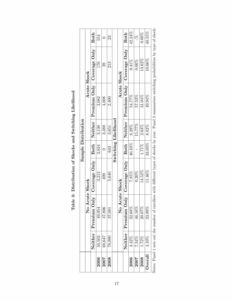
We investigate this hypothesis by considering three shocks to the consumer’s own characteristics
that could prompt her to incur the costs of search: two types of bad news concerning her current
plan’s characteristics for next year (the plan’s premium will rise or coverage will fall noticeably) and
an unusually high OOP payment driven by a health shock. We define a shock to premiums in the
enrollee’s current plan (vp) as a premium increase of more than the weighted median increase in the
relevant year. A coverage shock (vc) is defined as the plan dropping coverage in the coverage gap or
moving from the defined standard benefit to a different (tiered) system in the Pre-ICL phase. An
enrollee is defined as having an acute shock (vh) when she is in the top quintile of total drug cost
as well as the top decile of either percent spending on acute drugs or deviation between predicted
and observed spending. The distribution of these shocks in the population and their correlation
with the decision to switch plans are shown in Table 3.20 These three shocks appear to explain
switching behavior well. Those who receive no shocks switch very infrequently, only 4% of the
time, while those who receive multiple shocks are much more likely to switch plans21. Almost all
switchers (87%) receive some shock in the year of the switch.
We present further evidence in support of consumer inattention in Appendix C. In particular,
Table C4 sets out probit regressions of decision to switch plans on own-plan, low-cost plan and
personal characteristics. The estimates suggest that consumers’ switching probabilities increase
when their own plans’ premiums and OOP costs rise, but we find no evidence that consumers
respond to changes in premiums and costs for the lowest-cost plan available, the lowest-cost plan
within-brand, or the average of the five lowest-cost plans.
6.1 Consumer Demand Model
We specify a simple two-stage model of consumer decision-making with inattention. We assume
that each consumer i, once enrolled in a plan, ignores the choice problem until hit by a shock to the
OOP costs of her current plan or to her health. We consider the same three shocks vp, vc, vh defined
above; these are assumed to have additively separable effects on her decision to re-optimize her plan
choice. Additionally, the consumer could simply receive a random shock that causes awareness, for
example from a younger relative visiting the consumer and reviewing her plan choices. We label
this shock ve. The sum of these shocks creates a composite shock received by consumer i at time t:
vi,t = vi,p,tβ1 + vi,c,tβ2 + vi,h,tβ3 + vi,e,t (1)
20The acute shock has a cross-year correlation of around .5, which is considerably lower than the cross-year corre-lation of other measures of sickness. Total spending, total supply, and acute supply each have a cross-year correlationbetween .8 and .9, implying that the acute shock is substantially less persistent than underlying health status.
21These findings are corroborated by Hoadley et al. (2013), who find that premium increases and removal of gapcoverage are the best predictors of switching behavior.
16
Tab
le3:
Dis
trib
uti
on
of
Sh
ock
san
dS
wit
chin
gL
ikelih
ood
Sam
ple
Dis
trib
uti
on
No
Acu
teS
hock
Acu
teS
hock
Neit
her
Pre
miu
mO
nly
Covera
ge
On
lyB
oth
Neit
her
Pre
miu
mO
nly
Covera
ge
On
lyB
oth
2006
50,5
03
49,9
543,
212
2,82
43,
138
3,08
217
0554
2007
68,6
47
47,8
0649
90
3,48
84,
008
390
2008
78,9
80
37,0
815,
640
643
3,65
12,
400
213
23
Sw
itch
ing
Lik
eli
hood
No
Acu
teS
hock
Acu
teS
hock
Neit
her
Pre
miu
mO
nly
Covera
ge
On
lyB
oth
Neit
her
Pre
miu
mO
nly
Covera
ge
On
lyB
oth
2006
3.4
2%
32.6
8%
7.85
%40
.16%
8.29
%54
.77%
9.4
1%42
.24%
2007
7.3
4%
46.1
6%
0.20
%-
15.7
7%57
.53%
0.0
0%-%
2008
1.7
2%
20.0
7%
14.5
2%
1.71
%2.
63%
31.0
4%13.
62%
0.00
%
Overa
ll4.1
0%
33.9
9%
11.4
6%
33.0
3%8.
82%
49.9
4%10.
66%
40.5
5%
Not
es:
Pan
el1
sets
out
the
nu
mb
erof
enro
llee
sw
ith
diff
eren
tty
pes
of
shock
sby
year.
Pan
el2
sum
mari
zes
swit
chin
gp
rob
ab
ilit
ies
by
typ
eof
shock
.
17
where the weights β allow the different shocks to have different effects on the propensity to search
(for example shocks to premiums may increase the likelihood of switching more than other shocks).
When the composite shock vi,t is large enough, i.e. when:
vi,t ≥ vi,t, (2)
then the consumer becomes aware and decides to re-optimize her plan election. Here vi,t is a
function of consumer demographics related to health status and sensitivity to changes in plan
characteristics: age groups, income quartiles, gender and race. We also include year fixed effects
in vi,t to account for differences in the environment (e.g. advertising, phyarmacy and government
outreach) across our three different enrollment periods.
The second stage of the model examines how consumers who have decided to re-optimize choose
whether to switch and to which plans. We assume that, once aware, consumer i makes a choice
from the full choice set (including her current plan) based on the following utility from choosing
plan j in year t:
ui,j,t = ˆTrOOP i,j,tβ1 + Premiumj,t[β2,1 + vi,p,tβ2,2] +Dedj,tβ3,1
+ Gapj,t[β4,1 + vi,c,tβ4,2 + vi,h,tβ4,3] +Xj,tβ5,i + εi,j,t
= δi,j,t + εi,j,t (3)
where expected chronic OOP spending excluding premium ( ˆTrOOP i,j,t) is calculated using the
method described above, Premiumj,t and Dedj,t are annual premiums and deductibles and Gapj,t
is an indicator for any coverage in the gap. Xj,t are non-price plan characteristics including brand
fixed effects (defined at the carrier rather than the plan level) and an indicator for enhanced plans
interacted with year fixed effects, and εi,j,t is an IID extreme value type 1 error term (assumed to
be independent of vi,e,t). We allow consumers prompted to search by shocks to premiums to place
additional weight on premiums. Consumers experiencing shocks to coverage, or acute shocks, are
permitted to place additional weight on the plan offering gap coverage.
We model persistent unobserved preference heterogeneity by including normally-distributed
random coefficients β5,i on fixed effects for the three dominant brands, which together have over
80% market share in 2006, and on the enhanced plan fixed effect. The model therefore allows choice
persistence (such as a lack of switching away from a particular plan even when other plans reduce
their premiums) to be caused either by heterogeneous preferences (some consumers have a very
strong valuation for this brand that makes it worthwhile to remain enrolled even at a high relative
price) or by inattention (consumers who are not affected by any of the previously-defined shocks
are unaware of other plan premium reductions).
The model is estimated using a random coefficients simulated maximum likelihood approach
similar to that summarized in Train (2009). The likelihood function for each enrollee is predicted
for a sequence of choices from entry into the Part D program until the end of our data panel. A full
description of the empirical model is provided in Appendix D, where we also present estimates of
18
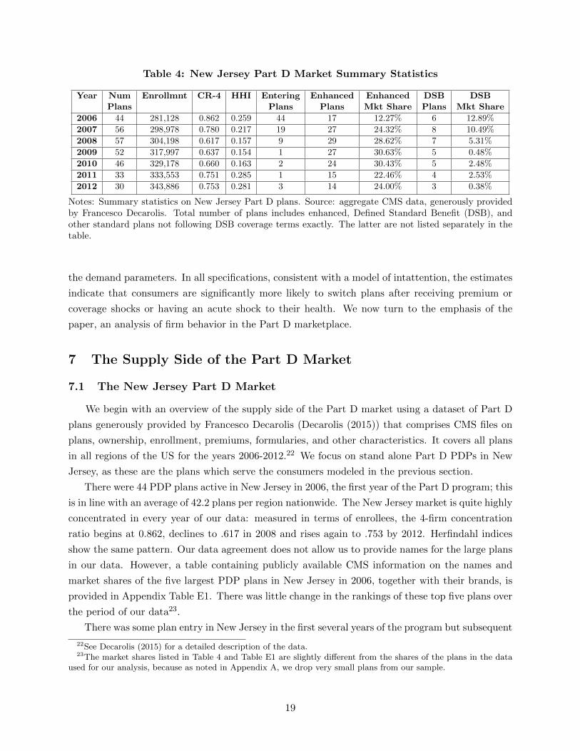
Table 4: New Jersey Part D Market Summary Statistics
Year Num Enrollmnt CR-4 HHI Entering Enhanced Enhanced DSB DSBPlans Plans Plans Mkt Share Plans Mkt Share
2006 44 281,128 0.862 0.259 44 17 12.27% 6 12.89%
2007 56 298,978 0.780 0.217 19 27 24.32% 8 10.49%
2008 57 304,198 0.617 0.157 9 29 28.62% 7 5.31%
2009 52 317,997 0.637 0.154 1 27 30.63% 5 0.48%
2010 46 329,178 0.660 0.163 2 24 30.43% 5 2.48%
2011 33 333,553 0.751 0.285 1 15 22.46% 4 2.53%
2012 30 343,886 0.753 0.281 3 14 24.00% 3 0.38%
Notes: Summary statistics on New Jersey Part D plans. Source: aggregate CMS data, generously providedby Francesco Decarolis. Total number of plans includes enhanced, Defined Standard Benefit (DSB), andother standard plans not following DSB coverage terms exactly. The latter are not listed separately in thetable.
the demand parameters. In all specifications, consistent with a model of intattention, the estimates
indicate that consumers are significantly more likely to switch plans after receiving premium or
coverage shocks or having an acute shock to their health. We now turn to the emphasis of the
paper, an analysis of firm behavior in the Part D marketplace.
7 The Supply Side of the Part D Market
7.1 The New Jersey Part D Market
We begin with an overview of the supply side of the Part D market using a dataset of Part D
plans generously provided by Francesco Decarolis (Decarolis (2015)) that comprises CMS files on
plans, ownership, enrollment, premiums, formularies, and other characteristics. It covers all plans
in all regions of the US for the years 2006-2012.22 We focus on stand alone Part D PDPs in New
Jersey, as these are the plans which serve the consumers modeled in the previous section.
There were 44 PDP plans active in New Jersey in 2006, the first year of the Part D program; this
is in line with an average of 42.2 plans per region nationwide. The New Jersey market is quite highly
concentrated in every year of our data: measured in terms of enrollees, the 4-firm concentration
ratio begins at 0.862, declines to .617 in 2008 and rises again to .753 by 2012. Herfindahl indices
show the same pattern. Our data agreement does not allow us to provide names for the large plans
in our data. However, a table containing publicly available CMS information on the names and
market shares of the five largest PDP plans in New Jersey in 2006, together with their brands, is
provided in Appendix Table E1. There was little change in the rankings of these top five plans over
the period of our data23.
There was some plan entry in New Jersey in the first several years of the program but subsequent
22See Decarolis (2015) for a detailed description of the data.23The market shares listed in Table 4 and Table E1 are slightly different from the shares of the plans in the data
used for our analysis, because as noted in Appendix A, we drop very small plans from our sample.
19
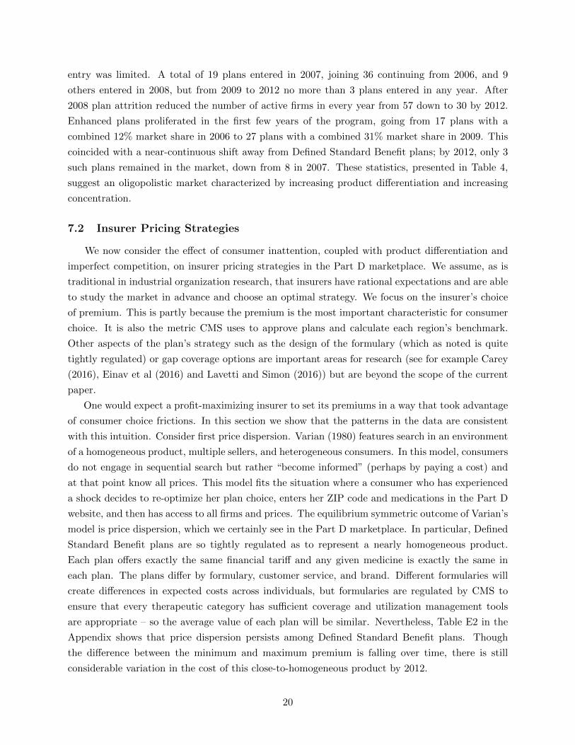
entry was limited. A total of 19 plans entered in 2007, joining 36 continuing from 2006, and 9
others entered in 2008, but from 2009 to 2012 no more than 3 plans entered in any year. After
2008 plan attrition reduced the number of active firms in every year from 57 down to 30 by 2012.
Enhanced plans proliferated in the first few years of the program, going from 17 plans with a
combined 12% market share in 2006 to 27 plans with a combined 31% market share in 2009. This
coincided with a near-continuous shift away from Defined Standard Benefit plans; by 2012, only 3
such plans remained in the market, down from 8 in 2007. These statistics, presented in Table 4,
suggest an oligopolistic market characterized by increasing product differentiation and increasing
concentration.
7.2 Insurer Pricing Strategies
We now consider the effect of consumer inattention, coupled with product differentiation and
imperfect competition, on insurer pricing strategies in the Part D marketplace. We assume, as is
traditional in industrial organization research, that insurers have rational expectations and are able
to study the market in advance and choose an optimal strategy. We focus on the insurer’s choice
of premium. This is partly because the premium is the most important characteristic for consumer
choice. It is also the metric CMS uses to approve plans and calculate each region’s benchmark.
Other aspects of the plan’s strategy such as the design of the formulary (which as noted is quite
tightly regulated) or gap coverage options are important areas for research (see for example Carey
(2016), Einav et al (2016) and Lavetti and Simon (2016)) but are beyond the scope of the current
paper.
One would expect a profit-maximizing insurer to set its premiums in a way that took advantage
of consumer choice frictions. In this section we show that the patterns in the data are consistent
with this intuition. Consider first price dispersion. Varian (1980) features search in an environment
of a homogeneous product, multiple sellers, and heterogeneous consumers. In this model, consumers
do not engage in sequential search but rather “become informed” (perhaps by paying a cost) and
at that point know all prices. This model fits the situation where a consumer who has experienced
a shock decides to re-optimize her plan choice, enters her ZIP code and medications in the Part D
website, and then has access to all firms and prices. The equilibrium symmetric outcome of Varian’s
model is price dispersion, which we certainly see in the Part D marketplace. In particular, Defined
Standard Benefit plans are so tightly regulated as to represent a nearly homogeneous product.
Each plan offers exactly the same financial tariff and any given medicine is exactly the same in
each plan. The plans differ by formulary, customer service, and brand. Different formularies will
create differences in expected costs across individuals, but formularies are regulated by CMS to
ensure that every therapeutic category has sufficient coverage and utilization management tools
are appropriate – so the average value of each plan will be similar. Nevertheless, Table E2 in the
Appendix shows that price dispersion persists among Defined Standard Benefit plans. Though
the difference between the minimum and maximum premium is falling over time, there is still
considerable variation in the cost of this close-to-homogeneous product by 2012.
20

Table 5: Average Premium Increase and % of Plans with $10 Premium Increase
Premium Increase ≥ $10 Premium Increase
Equal Equal Weighted Weighted Equal Equal Weighted WeightedBasic Enhanced Basic Enhanced Basic Enhanced Basic Enhanced
2007 -$2.94 $1.01 -$2.20 $7.20 33.33% 40.74% 0.33% 10.53%
2008 $4.65 $11.50 $5.93 $14.45 39.29% 55.17% 24.10% 39.82%
2009 $6.20 $7.12 $3.68 $4.39 24.00% 33.33% 0.83% 39.31%
2010 $5.06 $1.77 $2.92 $5.44 21.74% 29.17% 1.19% 35.08%
2011 $1.04 $14.33 -$3.09 $2.84 11.11% 73.33% 6.50% 24.48%
2012 -$1.24 $6.52 $1.97 $2.02 12.50% 42.86% 0.16% 16.38%
Notes: Summary of premium changes ($ per enrollee per month) over time for New Jersey PDPs, by Yearand Plan Type
As discussed in Section 4, consumer inertia is likely to have the effect of increasing equilbrium
price levels and creating an upward slope to prices. The upward trend may not be a steady-state
phenomenon; it occurs because the entire market begins in 2006. Thus every plan faces only
elastic choosers in that year and no locked in base. Table 5 shows that, consistent with these
predictions, premiums increase on average almost every year from 2007-12. The average annual
premium increase for basic plans (weighted by enrollment) is small, less than $6 per month in every
year. Premiums for enhanced plans increase more quickly; in 2008, the weighted-average premium
increase for enhanced plans is over $14 per month, and in 2011 and 2012 smaller enhanced plans
post large premium increases. The second panel of Table 5 flags plans that raise premiums by more
than $10. For three years from 2008 to 2010, at least a third of enrollees in enhanced plans face
large premium shocks, although the rate is lower in other years.
We can also use the intuition from the theory to predict differences in premium growth across
insurers. First, the change in profit for a given change in price is a function of both the intensive
margin (profit per enrollee) and the extensive margin (number of enrollees). Since larger firms
have a larger intensive margin, we should expect large firms to raise prices more than smaller firms
all else equal. Second, we should expect slower premium growth when the number of consumers
purchasing for the first time is high relative to the size of the installed base. Thus premiums should
rise more slowly in years with high attrition (e.g. high death rates) or large cohorts aging into the
Part D program.24 We estimate regressions of annual premium increases on lagged market shares,
growth rates, and other plan variables that might affect costs for all PDP plans in the national
dataset.
Table 6 reports the results of the main specification. When we control for region and carrier
fixed effects and coverage variables that may affect costs, lagged market shares significantly predict
future increases in premiums, providing evidence in support of the first hypothesis. The estimates
also indicate that the growth rate of enrollment in the region, which we treat as a proxy for new
24Because of our focus on shocks to consumers’ attention and the dynamics of pricing, we do not estimate ourmotivating regression in levels like Polyakova (2016), but rather in premium changes. It is the increase in price thatbecomes more lucrative with an increase in installed base.
21
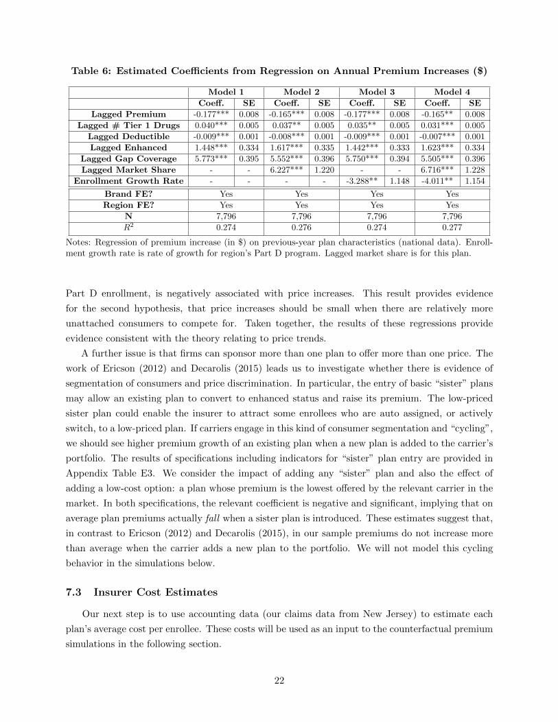
Table 6: Estimated Coefficients from Regression on Annual Premium Increases ($)
Model 1 Model 2 Model 3 Model 4
Coeff. SE Coeff. SE Coeff. SE Coeff. SE
Lagged Premium -0.177*** 0.008 -0.165*** 0.008 -0.177*** 0.008 -0.165** 0.008
Lagged # Tier 1 Drugs 0.040*** 0.005 0.037** 0.005 0.035** 0.005 0.031*** 0.005
Lagged Deductible -0.009*** 0.001 -0.008*** 0.001 -0.009*** 0.001 -0.007*** 0.001
Lagged Enhanced 1.448*** 0.334 1.617*** 0.335 1.442*** 0.333 1.623*** 0.334
Lagged Gap Coverage 5.773*** 0.395 5.552*** 0.396 5.750*** 0.394 5.505*** 0.396
Lagged Market Share - - 6.227*** 1.220 - - 6.716*** 1.228
Enrollment Growth Rate - - - - -3.288** 1.148 -4.011** 1.154
Brand FE? Yes Yes Yes Yes
Region FE? Yes Yes Yes Yes
N 7,796 7,796 7,796 7,796
R2 0.274 0.276 0.274 0.277
Notes: Regression of premium increase (in $) on previous-year plan characteristics (national data). Enroll-ment growth rate is rate of growth for region’s Part D program. Lagged market share is for this plan.
Part D enrollment, is negatively associated with price increases. This result provides evidence
for the second hypothesis, that price increases should be small when there are relatively more
unattached consumers to compete for. Taken together, the results of these regressions provide
evidence consistent with the theory relating to price trends.
A further issue is that firms can sponsor more than one plan to offer more than one price. The
work of Ericson (2012) and Decarolis (2015) leads us to investigate whether there is evidence of
segmentation of consumers and price discrimination. In particular, the entry of basic “sister” plans
may allow an existing plan to convert to enhanced status and raise its premium. The low-priced
sister plan could enable the insurer to attract some enrollees who are auto assigned, or actively
switch, to a low-priced plan. If carriers engage in this kind of consumer segmentation and “cycling”,
we should see higher premium growth of an existing plan when a new plan is added to the carrier’s
portfolio. The results of specifications including indicators for “sister” plan entry are provided in
Appendix Table E3. We consider the impact of adding any “sister” plan and also the effect of
adding a low-cost option: a plan whose premium is the lowest offered by the relevant carrier in the
market. In both specifications, the relevant coefficient is negative and significant, implying that on
average plan premiums actually fall when a sister plan is introduced. These estimates suggest that,
in contrast to Ericson (2012) and Decarolis (2015), in our sample premiums do not increase more
than average when the carrier adds a new plan to the portfolio. We will not model this cycling
behavior in the simulations below.
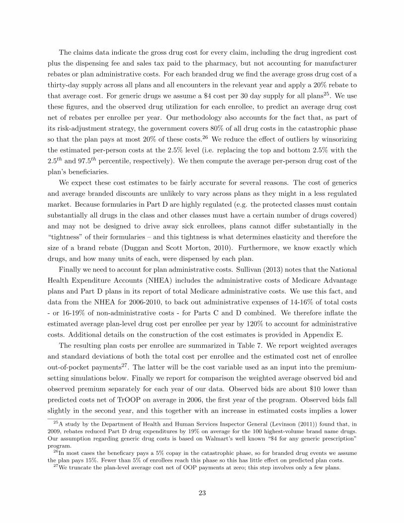
7.3 Insurer Cost Estimates
Our next step is to use accounting data (our claims data from New Jersey) to estimate each
plan’s average cost per enrollee. These costs will be used as an input to the counterfactual premium
simulations in the following section.
22
The claims data indicate the gross drug cost for every claim, including the drug ingredient cost
plus the dispensing fee and sales tax paid to the pharmacy, but not accounting for manufacturer
rebates or plan administrative costs. For each branded drug we find the average gross drug cost of a
thirty-day supply across all plans and all encounters in the relevant year and apply a 20% rebate to
that average cost. For generic drugs we assume a $4 cost per 30 day supply for all plans25. We use
these figures, and the observed drug utilization for each enrollee, to predict an average drug cost
net of rebates per enrollee per year. Our methodology also accounts for the fact that, as part of
its risk-adjustment strategy, the government covers 80% of all drug costs in the catastrophic phase
so that the plan pays at most 20% of these costs.26 We reduce the effect of outliers by winsorizing
the estimated per-person costs at the 2.5% level (i.e. replacing the top and bottom 2.5% with the
2.5th and 97.5th percentile, respectively). We then compute the average per-person drug cost of the
plan’s beneficiaries.
We expect these cost estimates to be fairly accurate for several reasons. The cost of generics
and average branded discounts are unlikely to vary across plans as they might in a less regulated
market. Because formularies in Part D are highly regulated (e.g. the protected classes must contain
substantially all drugs in the class and other classes must have a certain number of drugs covered)
and may not be designed to drive away sick enrollees, plans cannot differ substantially in the
“tightness” of their formularies – and this tightness is what determines elasticity and therefore the
size of a brand rebate (Duggan and Scott Morton, 2010). Furthermore, we know exactly which
drugs, and how many units of each, were dispensed by each plan.
Finally we need to account for plan administrative costs. Sullivan (2013) notes that the National
Health Expenditure Accounts (NHEA) includes the administrative costs of Medicare Advantage
plans and Part D plans in its report of total Medicare administrative costs. We use this fact, and
data from the NHEA for 2006-2010, to back out administrative expenses of 14-16% of total costs
- or 16-19% of non-administrative costs - for Parts C and D combined. We therefore inflate the
estimated average plan-level drug cost per enrollee per year by 120% to account for administrative
costs. Additional details on the construction of the cost estimates is provided in Appendix E.
The resulting plan costs per enrollee are summarized in Table 7. We report weighted averages
and standard deviations of both the total cost per enrollee and the estimated cost net of enrollee
out-of-pocket payments27. The latter will be the cost variable used as an input into the premium-
setting simulations below. Finally we report for comparison the weighted average observed bid and
observed premium separately for each year of our data. Observed bids are about $10 lower than
predicted costs net of TrOOP on average in 2006, the first year of the program. Observed bids fall
slightly in the second year, and this together with an increase in estimated costs implies a lower
25A study by the Department of Health and Human Services Inspector General (Levinson (2011)) found that, in2009, rebates reduced Part D drug expenditures by 19% on average for the 100 highest-volume brand name drugs.Our assumption regarding generic drug costs is based on Walmart’s well known “$4 for any generic prescription”program.
26In most cases the beneficary pays a 5% copay in the catastrophic phase, so for branded drug events we assumethe plan pays 15%. Fewer than 5% of enrollees reach this phase so this has little effect on predicted plan costs.
27We truncate the plan-level average cost net of OOP payments at zero; this step involves only a few plans.
23
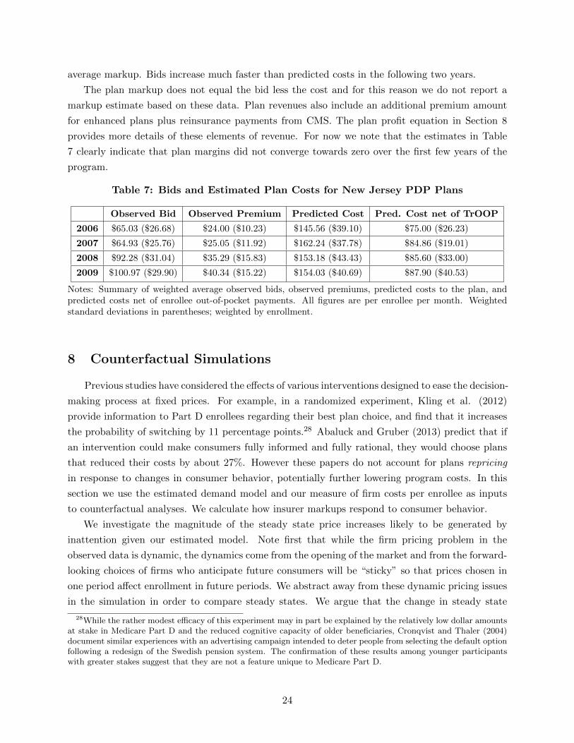
average markup. Bids increase much faster than predicted costs in the following two years.
The plan markup does not equal the bid less the cost and for this reason we do not report a
markup estimate based on these data. Plan revenues also include an additional premium amount
for enhanced plans plus reinsurance payments from CMS. The plan profit equation in Section 8
provides more details of these elements of revenue. For now we note that the estimates in Table
7 clearly indicate that plan margins did not converge towards zero over the first few years of the
program.
Table 7: Bids and Estimated Plan Costs for New Jersey PDP Plans
Observed Bid Observed Premium Predicted Cost Pred. Cost net of TrOOP
2006 $65.03 ($26.68) $24.00 ($10.23) $145.56 ($39.10) $75.00 ($26.23)
2007 $64.93 ($25.76) $25.05 ($11.92) $162.24 ($37.78) $84.86 ($19.01)
2008 $92.28 ($31.04) $35.29 ($15.83) $153.18 ($43.43) $85.60 ($33.00)
2009 $100.97 ($29.90) $40.34 ($15.22) $154.03 ($40.69) $87.90 ($40.53)
Notes: Summary of weighted average observed bids, observed premiums, predicted costs to the plan, andpredicted costs net of enrollee out-of-pocket payments. All figures are per enrollee per month. Weightedstandard deviations in parentheses; weighted by enrollment.
8 Counterfactual Simulations
Previous studies have considered the effects of various interventions designed to ease the decision-
making process at fixed prices. For example, in a randomized experiment, Kling et al. (2012)
provide information to Part D enrollees regarding their best plan choice, and find that it increases
the probability of switching by 11 percentage points.28 Abaluck and Gruber (2013) predict that if
an intervention could make consumers fully informed and fully rational, they would choose plans
that reduced their costs by about 27%. However these papers do not account for plans repricing
in response to changes in consumer behavior, potentially further lowering program costs. In this
section we use the estimated demand model and our measure of firm costs per enrollee as inputs
to counterfactual analyses. We calculate how insurer markups respond to consumer behavior.
We investigate the magnitude of the steady state price increases likely to be generated by
inattention given our estimated model. Note first that while the firm pricing problem in the
observed data is dynamic, the dynamics come from the opening of the market and from the forward-
looking choices of firms who anticipate future consumers will be “sticky” so that prices chosen in
one period affect enrollment in future periods. We abstract away from these dynamic pricing issues
in the simulation in order to compare steady states. We argue that the change in steady state
28While the rather modest efficacy of this experiment may in part be explained by the relatively low dollar amountsat stake in Medicare Part D and the reduced cognitive capacity of older beneficiaries, Cronqvist and Thaler (2004)document similar experiences with an advertising campaign intended to deter people from selecting the default optionfollowing a redesign of the Swedish pension system. The confirmation of these results among younger participantswith greater stakes suggest that they are not a feature unique to Medicare Part D.
24

outcomes is of most policy relevance for a program that is long-lived. We assume in our demand
model that attentive consumers are not forward-looking or strategic; rather, they choose the plan
they most prefer today based on today’s characteristics. (This seems very likely given what we
know about the sophistication of these consumers and their uncertainty about how the market
will develop in the future.) This estimation therefore yields preference parameters that are valid
representations of consumer behavior, regardless of the strategy the firms may be pursuing. We can
then use these preference parameters combined with our cost data to generate a variety of different
static equilibrium markups, corresponding to different levels of inattention and hence different
premium elasticities, using a simple system of static first-order conditions. We consider only non-
LIS enrollees and focus on the simple situation where consumer preferences are not affected by
shocks experienced in the previous year.
We focus on the premium markup for several reasons. First, the results of Abaluck and Gruber
and others indicate that consumers choose poorly in this marketplace and are unable to properly
weight attributes of a plan such as out of pocket costs and deductibles. Consumers often choose
plans based largely on the premium. Our demand estimates are consistent with this finding, im-
plying that removing inattention (without addressing other choice frictions) would affect consumer
sensitivity to premiums much more than their response to out of pocket costs. That is, we focus on
the plan characteristic that is most likely to respond to the removal of inattention. Further, basic
plans are constrained to offer a tariff that is actuarially equivalent to that set out in the law, so they
are financially fairly homogeneous to the average consumer except for the premium. While insurers
may design the formulary, and hence out-of-pocket payments, of their plans (particularly enhanced
plans) in a strategic way to influence enrollee choices and utilization, the plan’s bid is the choice
over which it has most discretion and the one that feeds directly into the premium calculation and
therefore its competitiveness in the marketplace. We focus on this choice, leaving issues related to
formulary design for future research.29
We begin by predicting plans’ optimal premiums in the simple scenario of full attention; details
of our method are provided in Section 8.1. The next step is to use the premium, coverage and acute
health shocks observed in the data (generated by realized plan premium and coverage changes) to
calculate the proportion of consumers that our model (equation (2)) predicts will be attentive
in each year. For example, the shocks in the data imply that 37% of consumers will reoptimize
in 2007, while 100% are assumed to optimize in 2006. We assume that attentive consumers make
choices to maximize the estimated utility equation (3) while inattentive consumers have a zero price
coefficient in that equation. This provides a simple way to translate the “probability of attention”
implied by the mix of attentive and inattentive consumers in the data into an expected premium
sensitivity that is faced by insurers.30 It is then straightforward to repeat the exercise of predicting
29Papers such as Carey (2016), Einav et al (2016) and Lavetti and Simon (2016) consider strategic factors affectinginsurers’ formulary choices in Part D.
30We generate a new utility equation that is the same as equation (3) except that the premium coefficient is scaledby the percent of consumers who are attentive. It would be more accurate to assume that inattentive consumers hada zero price elasticity, but this would substantially complicate the simulations.
25
equilibrium premiums using static first order conditions given the new (less negative) premium
coefficient.
This method abstracts away from several complicating factors. First, as noted, our desired
simulation does not require us to address dynamics at all. Secondly, we do not compare our
simulated outcomes to data because the data contain in them the impact of the dynamics—which
might lower the absolute level of markups in early years, for example—and therefore are not directly
comparable to our predictions. Our objective is to provide an approximate magnitude of the
impact of consumer inattention on the steady state markup. We therefore calculate a range of
possible premium effects under different assumptions regarding the mix of attentive and inattentive
consumers in the population. As we vary the proportion of consumers who are attentive, we vary
the price elasticity of demand facing the insurer, and hence its incentive to choose a particular
premium level. We assess the range of likely premium effects of inattention by reporting predicted
consumer spending when the percent attentive varies between 20% and 80% of the population.
A second caveat is that we do not model each individual plan at the micro level to make the link
between that plan’s premium choice and the attentiveness of its own incumbent enrollees. That
is, our analysis does not model the strategy of each plan to raise premiums and lose some (newly
attentive) consumers. We instead assume a population-level probability of consumer attentiveness,
and then calculate premiums that generate an equilibrium at the population level. Our preferred
method uses an iterative algorithm to address the issue that the premiums chosen by particular
plans may generate premium increases (and hence shocks) that affect the proportion of enrollees
choosing to re-optimize, implying that assuming a fixed probability of attentiveness to which plans
respond when choosing premiums may generate predictions that are internally inconsistent. Our
iterative algorithm proceeds as follows. The predicted premium choices in iteration k are used
to generate predicted premium shocks and therefore a probability of attentiveness (from equation
(2)) and new premium coefficient (in equation (3)). That premium coefficient is used to predict
new premium choices in iteration k + 1. We repeat until convergence, thereby ensuring that the
population percent attentive is consistent with the proportion of plans generating premium shocks.
We note that some price changes over time are predicted in our simulations, despite their being
a steady state exercise. We do not mean these to be interpreted as “dynamics.” Rather, they are
changes in static predictions that occur due to changing inputs, such as underlying plan costs, and
to the fact that the proportion of enrollees new to Part D differs by year. For example, premiums
are predicted to be low in 2006 in every simulation, since all consumers are new to the market in
that first year and therefore are assumed to be attentive.
We now discuss the possible sources of error in our approach. As noted above, we expect our
approximation of costs to be fairly accurate. Any mismeasurement would in any case be likely to
affect cost levels rather than the differences across our simulations. Second, our model does not
account for the possibility that consumers may in fact be forward-looking, choosing plans with
relatively high prices because they expect those plans to have lower prices in the future when they
are inattentive. However, there is a large amount of research into the behavior of Part D consumers,
26
none of which indicates that this kind of forward-looking planning is probable. Third, there might
be a steady state that is a perpetual cycle (perhaps with entry and price changes, or LIS cycling as
in Decarolis 2015) and not the static outcome we simulate. Our approach also abstracts away from
other reasons why premiums might change over time, including insurer learning and low pricing in
early years to attract enrollees with the goal of switching them to MA plans. While these dynamic
effects are certainly possible, we showed in Section 7 that we found no evidence of premium cycling
in response to sister plan entry in our sample. Further, we argue that short-term issues such as plan
learning are of second-order importance for the steady state premium effect of inattention that is
our focus.
An alternative approach to our counterfactuals would have been to simulate the dynamic path
of premiums in the baseline model with inattention. However, predicting the equilibrium of a
dynamic pricing game with many firms is difficult. Papers on the methodological frontier have
either considered very simple markets with two firms and small numbers of consumer types (e.g.
Dube et al (2010)) or made other simplifying assumptions, e.g. of a finite time horizon, or the
simplification that markets are large enough that the random evolution of individual firms “averages
out” and each firm can be assumed to respond to a long-run average industry state rather than the
predicted current choices of its competitors (Weintraub et al (2008) and applications such as Miller
(2014)). None of these assumptions seems reasonable in our setting. We argue that our simulations
provide a reasonable first approximation to the substantial cost savings, for both consumers and
the federal government, that could arise from policies to increase consumer attentiveness. We leave
the specification and estimation of a dynamic premium-setting model as an important path for
future research.
8.1 Counterfactual Details
We simulate consumer and plan choices using the fixed sample of 40 New Jersey PDP plans that
entered the market in 2006; we follow each plan through to its exit from the market.31 By limiting
ourselves to these 40 plans we ensure that the reported numbers focus only on within-plan price
and spending changes.
Recall that each insurer submits a bid for each plan. That bid determines the price consumers
face (the amount over the base beneficiary premium). This institutional reality requires us to
reframe the static price-setting game that is standard in the industrial organization literature as a
game where insurers choose bids given a prediction of the implications for the premiums faced by
consumers. Importantly, each basic plan must offer actuarially equivalent coverage if it does not
follow the tariff set out by law. This means that for a statistical person, the mean of OOP charges
must be the same in expectation for all basic plans, so plans cannot respond to increased consumer
premium sensitivity by reducing premiums while increasing average OOP charges. Additionally, the
subsidy for each enrollee is risk-adjusted depending on age, chronic conditions, LIS, and institutional
31There were actually 44 PDP plans in New Jersey in 2006 (Table 4); as noted in Appendix A, we drop the smallestplans in the sample, so we focus on 40 of these 44. 31 of the 40 plans were still active in 2009.
27
status. While the risk-adjustment mechanism is potentially manipulable, risk-adjusted subsidies
plus the high share of catastrophic costs paid by CMS (80%) mean it will be difficult for firms to
immediately determine whether particular enrollees are profitable or not, and the computation will
be complex. We therefore abstract from selection issues as we model the behavior of insurers. We
model insurers’ choices of bids while holding the schedule of OOP charges fixed.
We write plan j’s variable profit in year t as:
πj,t = (Bj,t + Ej,t − Cj,t)Nj,t (4)
where Bj,t is the bid made to CMS reflecting the plan’s average monthly revenue requirement per
enrollee in a basic plan (including profit), Ej,t is the additonal amount charged to enrollees in an
enhanced plan (the “enhanced premium”; this is zero when j is a basic plan), Cj,t is the plan’s cost
per enrollee net of enrollee OOP payments and Nj,t is its number of enrollees.
The premium charged to enrollees in a basic plan is the difference between the bid and the
proportion of the NAMBA that is subsidized by the government:
PremiumBasicj,t = Bj,t − γtNAMBAt = (1− γt
Jt)Bj,t −
γtJt
Σk 6=jBk,t (5)
where γt is the proportion of the NAMBA that is paid by the government and Jt is the number of
Part D plans included in the average in year t.32 This expression reflects the fact that, in the first
two years of the program, the NAMBA was an unweighted national average of bids for all MA and
PDP plans. From 2008 on, CMS phased in the implementation of a weighted average, where the
weight was the plan’s enrollment.33
We take several steps to account for CMS’s risk adjustment strategy. The government subsidy,
which is written into law at 74.5% of the NAMBA, is split between a premium subsidy and reinsur-
ance or risk adjustment payments. The latter include a commitment to pay 80% of the total cost
of drugs above each enrollee’s catastrophic threshold and payments to keep plans within symmetric
risk corridors that limit their overall losses and profits. We adjust our measure of plan costs per
enrollee to take account of the catastrophic drug subsidies as described in the previous section. We
use the true proportion of the NAMBA that is paid by the government in every year (which is
observed in our data, e.g. 66% in 2006) as an input to the premium calculation in equation (5).
We assume that the remaining risk adjustment payments offset the effect of enrollee selection on
plan costs, i.e. the cost per enrollee does not change with enrollees’ plan choices in our simulations.
32CMS requires that the basic premium never fall below zero. Our simulations account for this constraint. Howeverwe note that the constraint is not binding for PDPs in our data, although MA-PDs, which bundle prescription druginsurance with Medicare Part C insurance and whose bids are included in the NAMBA, often have very low premiumbids.
33The premium charged to enhanced plan enrollees is the basic premium defined in equation (5) plus the enhancedpremium Ej,t. The enhanced premium is negotiated between the carrier and CMS and is meant to comprise theaverage additional cost of enhanced benefits provided to enrollees in the plan. It is not subsidized by CMS. Weobserve this variable in the data for every plan-year and account for it in our simulations under the assumption thatit does not change in response to changes in enrollee attention.
28
Under each counterfactual scenario we consider a single-stage consumer demand system. We
use the estimated parameters of the utility equation described in Section 6.1 (the full specification,
model 4 of Appendix Table D1) but set the coefficients on premium, coverage and acute health
shocks to zero. The premium coefficient is adjusted as described above to approximate the effect of
a particular mix of attentive and inattentive consumers on premium responsiveness. The resulting
utility equation can be written as:
ui,j,t = ˆTrOOP i,j,tβ1 + Premiumj,tβ2,1 +Dedj,tβ3,1 +Gapj,tβ4,1 +Xj,tβ5,i + εi,j,t
= λi,j,t(β5,i) + Premiumj,tβ2,1 + εi,j,t
= δi,j,t(β5,i) + εi,j,t (6)
where Premiumj,t includes the enhanced premium where relevant and β2,1 is adjusted across sim-
ulations. λi,j,t(.) includes all consumer and plan-specific variables in the estimated utility equation
except the premium; it is a function of β5,i, the random coefficients on the three dominant brands
and the interactions between enhanced plan and year fixed effects. This utility equation can be
used to predict plan enrollment Nj,t under any set of plan characteristics:
Nj,t =
Nt∑i=1
∫β5,i
eδi,j,t(β5,i)∑Jtk=1 e
δi,k,t(β5,i)∂F (β5,i)
=
Nt∑i=1
∫β5,i
Λi,j,t(λi,j,t(β5,i), λi,−j,t(β5,i), P remiumj,t, P remium−j,t) ∂F (β5,i). (7)
Here Λi,j,t(.) is the predicted probability that consumer i chooses plan j in period t; it is a
function of all plan characteristics including their premiums. We consider plans’ optimal choices in
the static bid-setting game. The first-order condition for plan profits with respect to the bid Bj,t
is:
(Bj,t + Ej,t − Cj,t)∂Nj,t
∂Bj,t+Nj,t = 0. (8)
Calculating the derivative∂Nj,t
∂Bj,trequires us to predict the effect of a change in the bid Bj,t on
the premium. We use the expression in equation (5) under the assumption that the NAMBA is an
(unweighted) national average for MA-PD and PDP plans and that plans internalize their impact
on the NAMBA, and therefore on the government subsidy, when choosing their bids34. We predict
34We account for the fact that a change in one plan’s bid will affect all plans’ premiums via the subsidy. We usenational NAMBA figures published in annual press releases as an input to this analysis. The bid-setting game issolved for New Jersey PDP plans, assuming that PDP plans outside NJ will change their bids proportionately withNJ PDP plans, but holding fixed the bids of MA plans both within and outside this state. See Appendix E for details.
29
the resulting effect on enrollment using equation (7). The first order condition simplifies to:
Nj,t + (Bj,t + Ej,t − Cj,t){
ΣNti=1 β2,1[
∫β5,i
Λi,j,t(.)(1− Λi,j,t(.)) ∂F (β5,i)]Jt − γtJt
+Σk 6=j β2,1[
∫β5,i
Λi,j,t(.)Λi,k,t(.) ∂F (β5,i)]γtJt
}= 0
where we omit the arguments of Λi,j,t(.) for ease of exposition. All plans’ bids enter this equation
through Λi,j,t(.) as well as through Bj,t. We solve this system of equations to obtain the implied
new equilibrium for bids. Additional details of this derivation are provided in Appendix E.
8.2 Counterfactual Results
Tables 8-10 report our results. Table 8 sets out the cross-enrollee average premium costs and OOP
spending (including premiums) predicted by our model with and without inattention. The first col-
umn shows the predictions under full attention. Column 2 (“Inattention (Using Observed Shocks)”)
shows the same simulated costs when the shocks observed in the data between 2006-2008 are used
to predict the proportion of consumers who are attentive the following year (given equation (2))
and the premium coefficient in equation (6) is scaled down accordingly. The proportion attentive
is reported in the column labeled “P(att’n)”. It equals 1 in 2006, the first year of the program;
predicted spending with and without inattention are equal in that year. In the subsequent three
years the percent attentive varies between 0.33-0.45. Premiums and OOP spending are lower under
full attention in each of these years for two reasons. First, plans reduce their premium bids in
response to the higher premium elasticity, generating a reduction in premiums charged. Second,
enrollees place a higher (negative) weight on premiums in the utility equation, and hence choose
lower-premium plans. These results indicate a large saving from the simulated change in elasticity
due to attention: a total out-of-pocket cost saving (including premiums) of $1,154.20 per enrollee
over three years or 25.6% of total spending.
The third column of Table 8, labeled “Inattention (Iterative Algorithm)”, contains our preferred
specification under inattention. As described above we begin with the outcome under “Inattention
(Using Observed Shocks)” and iterate, predicting the shocks in iteration k using premiums gener-
ated in iteration k − 1, and repeating until convergence. Thus the predicted premiums reported
in this column are consistent with the proportion of consumers assumed to be attentive (i.e. the
proportion with a non-zero premium coefficient). The results change only slightly: the probability
of attention is slightly higher than in column 2, varying from 0.38-0.42 in the years 2007-9, and the
corresponding consumer spending is slightly lower. Savings from a move to full attention are now
$1,051.90 or 23.9% of total spending.
Table 9 sets out additional robustness tests in the spirit of providing a range of estimates of the
effect of consumer inattention. We report consumer spending under different assumed proportions
of attentive and inattentive consumers in the population: we allow the proportion attentive to vary
from 0.2 to 0.8, in increments of 0.2. The estimates are intuitive. The higher the proportion atten-
30

Table 8: Simulated Per-Person Spending With Premium Adjustments
Full Attention Inattention Inattention(Using Observed Shocks) (Iterative Algorithm)
Premium OOP Premium OOP P(att’n) Premium OOP P(att’n)
2006 $190.19 $1,111.90 $190.19 $1,111.90 1 $190.19 $1,111.90 1
2007 $263.62 $1,149.00 $678.26 $1,545.80 0.37 $611.49 $1,480.30 0.42
2008 $253.76 $1,075.00 $750.71 $1,545.40 0.33 $659.98 $1,457.20 0.38
2009 $275.53 $1,135.40 $596.45 $1,422.40 0.45 $650.67 $1,473.80 0.41
Total ’07-09 $792.91 $3,359.40 $2,025.42 $4,513.60 $1,922.14 $4,411.30
Spending above $1,154.20 $1,051.90Full Attention
% Difference 25.6% 23.9%
Notes: Results of simulations allowing premiums to adjust to changes in consumer behavior. Predicted OOPcosts are cross-enrollee averages per enrollee per year including premiums. “Full Attention” assumes allconsumers make a new choice every year. “Inattention (Using Observed Shocks)” uses observed shocks toinfer percent of attentive consumers and implied premium coefficient. “Inattention (Iterative Algorithm)”iterates to a point where predicted premium increases consistent with percent attentive consumers.
Table 9: Simulated Per-Person Spending, Robustness
P(att’n)=0.2 P(att’n)=0.4 P(att’n)=0.6 P(att’n)=0.8
Premium OOP Premium OOP Premium OOP Premium OOP)
2007 $1,128.50 $1,991.00 $639.37 $1,507.60 $445.11 $1,318.30 $337.10 $1,215.90
2008 $1,159.30 $1,947.60 $633.46 $1,431.50 $430.88 $1,237.80 $320.36 $1,134.90
2009 $1,153.70 $1,964.50 $661.66 $1,484.30 $464.54 $1,299.60 $351.14 $1,198.90
Total ’07-09 $5,903.10 $4,423.40 $3,890.90 $3,549.70
Spending above $2,543.70 $1,064.00 $496.30 $190.30Full Attention
% Difference 43.1% 24.1% 12.9% 5.4%
Notes: Predicted OOP costs are cross-enrollee averages per enrollee per year including premiums. Premiumsinclude both basic and enhanced premium. Each column assumes a different percent of consumers who areattentive, and hence a different premium coefficient in utility equation.
tive, the higher the effective premium elasticity, and the lower is consumer spending on premiums,
both because plans adjust their premiums strategically and because consumers increasingly prefer
low-premium plans. The relationship between percent attentive and total consumer spending is
not linear: the spending reductions fall with each incremental increase in percent attentive. This
is unsurprising because the premium coefficient is one input into a non-linear choice model that
determines plan market shares and hence both bids and consumer spending. However, it is clear
that the higher the initial percent attentive, the lower the saving from removing inattention. The
estimates range from a 43% saving if only 20% of consumers are initially attentive, to a 5% saving
if the initial proportion is 80%.
Table 10 reports the cross-plan unweighted average bids (the NAMBA) that generate the pre-
miums reported in Table 8, with and without inattention. Since we assume that all consumers
are attentive in 2006, the same average bid—$1027.40 per enrollee per year—is predicted in both
columns 1 and 2 of the table (“attentive” and “inattentive”). In later years, as expected, average
bids are lower when all consumers are assumed to be attentive (column 1) than under our preferred
31

Table 10: Government Savings from Repricing Due to Full Attention
Year NAMBA: NAMBA: γt Annual ($) Non-LIS SavingsFull Att’n Inattention Savings / Enr Enrollment ($ million)
2006 $1,027.40 $1,027.40 0.65
2007 $964.30 $1,061.50 0.66 $64.15 8,120,524 $521 million
2008 $971.90 $1,049.80 0.65 $50.88 8,413,202 $428 million
2009 $1,001.20 $1,071.50 0.64 $44.99 8,572,910 $386 million
Total ’07-09 $1,335 million
Notes: Results of Program Cost Savings Calculation. Columns 1 and 2 are predicted unweighted nationalaverage bids, PDP and MA plans nationally, measured in $ per year. We use the iterative algorithmcorresponding to column 3 of Table 8 to simulate inattention. Per-enrollee average savings are the differencebetween the two average bids scaled by the proportion paid by the government. Non-LIS enrollment reportedin national plan data generously provided by Francesco Decarolis. γt is defined in Section 8.
iterative algorithm for inattention (column 2). For example, in 2007, the predicted NAMBA under
full attention is $964.30 per enrollee per year, while under inattention the corresponding figure
is $97 higher at $1,061.50. The difference varies over years, with changes in plan costs and the
observed enhanced premium, but it is greater than six percent of the “inattention” level in every
year 2007-9.35 Finally, we note that the unweighted national average NAMBA observed in the
data for 2006 is $1,108; it varies between $965 and $1,110 in the years 2007-9. While plan dynamic
choices are likely to generate changes over time that we do not expect our simulations to match,
the fact that the difference between observed and predicted NAMBA is never more than 9% of our
simulated estimate is evidence of the accuracy of our cost measures.36
If we are willing to assume that our New Jersey estimates can be extrapolated to the entire
nation, we can use the predicted bids to calculate the implied government savings for enrolled
consumers over the years 2007-9. These savings are substantial. Program cost savings result
from the reduction in plan bids, of which the government pays a sizeable proportion. Applying the
conservative assumption that reinsurance costs remain fixed so that the government saves a fraction
of the difference in average bids equal to one minus the Base Beneficiary Percentage (γt in equation
(5)), we find that government savings amount to between $45 and $64 per covered life per year in the
years 2007-9. Assuming further that low-income subsidy payments are unaffected and multiplying
this figure by the non-LIS PDP population in each year generates an estimate of the government’s
total savings from reduced bids. We predict savings of $1.3 billion or 1% of the government’s cost
of this part of the program over the three years 2007-9.37 This is a conservative estimate: we use
35The reductions in bids reported here are smaller than the reductions in consumer spending due to endogenousconsumer choice. The Table 10 bid numbers are unweighted averages across plans, consistent with the method usedto calculate government program costs in the first few years of the program. In contrast Table 8 reports averagesacross enrollees rather than plans. Consumers tend to choose lower-premium plans, particularly in the “full attention”simulations when the premium coefficient is most negative.
36These reported observed NAMBAs are unweighted national averages, while those in Table 7 are enrollment-weighted averages for NJ PDPs only (reported in $ per month for comparison with our cost estimates).
37This simple calculation assumes that, if inattention is removed nationally, the reduction in bids for PDP plansoutside New Jersey will be the same as the average predicted reduction in NJ PDP plan bids, while MA plan bids
32
unweighted average bids, consistent with the use of unweighted averages to calculate the NAMBA
in the first few years of the program, so our projections do not account for the impact on the
weighted NAMBA of differential enrollee sorting into low-cost plans when bids change.38 Clearly
we have made multiple assumptions to arrive at these numbers. However, when combined with
the theoretical results discussed in Section 4, our estimates are sufficient to provide clear evidence
that removing inattention would lead to substantial savings both to the federal government and to
consumers.
The CBO calculated that from 2007-10 the cost of the drug component of the basic benefit
increased by 2.8% per annum on average for Part D enrollees while administrative costs and profits
rose at 6.7%.39 Premiums increased from a weighted average of $25.93 to $37.25 from 2006 to
2010 according to the Kaiser Family Foundation (Hoadley (2015)). This is the environment we
explore with our data and seek to explain as rational pricing in the face of consumer inattention.
Interestingly, the environment changed significantly in the second five years of the program. From
2010 to 2014 the rate of generic penetration increased significantly and the introduction of new
branded blockbuster drugs slowed. National pharmaceutical expenditure actually fell in nominal
terms in 2012 and 2013 according to IMS data (Schumock et al (2014)). However, from 2010 to
2015 stand alone Part D premiums stayed approximately constant at between $37.02 and $38.54
(Hoadley (2015)). Because drug costs fell modestly in those years, it is not clear what happened to
the margins of the insurers participating in Part D. Ideally, effective regulation should ensure that
costs are reflected in prices. That is, falling drug costs should benefit consumers in the form of falling
premiums if a program is delivering the competitive benefits society expects. The available evidence
suggests that this did not happen, adding weight to our hypothesis that consumer inattention
limits the effectiveness of competition in this market. It may be the case that the underlying cost
environment has changed again recently, as several sources report significant increases in specialty
drug spending for 2014.40 Further research into the impact of consumer choice in Part D on
competition is clearly warranted.
9 Conclusions
In this paper we have developed a model of consumer choice in the Part D program and have
analyzed how firms set prices in response to the presence or absence of consumer inattention. The
data support a model where consumers face costs of processing information. This leads them to
avoid making new choices, rolling over their plan selections from one year to the next unless shocked
by a change to their current plan or their current health.
remain constant. The $1.3 billion saving is 1% of the government’s cost of subsidizing PDP premiums for non-LISenrollees nationally.
38This is the primary reason why the predicted government saving is lower than the weighted average saving toconsumers from removing inattention. A second reason for the difference in percent savings is that the denominatorfor the government is the total cost of subsidizing PDP premiums, including risk payments and reinsurance, whilefor the consumer it is simply out-of-pocket payments.
39Figure 2-1 page 21 CBO report “Competition and the Cost of Medicare’s Prescription Drug Program 2014”.40e.g. Express Scripts 2014 Drugs Trend Report.
33
We provide evidence that firms’ premium choices are responsive to consumers’ search frictions.
In particular, when consumers are attentive, firms are incentivized to lower their margins, resulting
in lower premiums. Using our estimates of consumer behavior and a model of firm price-setting
we use a simple approach to approximate the steady state effects of consumer inattention on
premiums charged and consumer spending. We predict a large price response to full consumer
attention because, in that environment, an effective way for plans to attract customers is by lowering
premiums. Our simulations indicate that the combination of the demand- and supply-side changes
would reduce the amount consumers spend by 24%. The natural plan response of increasing other
components of the price, like the OOP cost schedule, is constrained by the quite tightly regulated
standard benefit levels.
We do not consider price dynamics. We note that theory predicts an increasing path of prices,
particularly in early years of the program, as plans respond to incentives to “invest” in new enrollees
and then “harvest” their installed based; this implies that the price effects of inattention may be
increasing over time. However there are also other, potentially offsetting effects, such as insurer
learning about the Part D environment during the first few years of the program. Steady state
equilibria could also involve plans cycling between high and low prices, particularly in situations
where several plans are offered by a single insurer. Our simulations do not capture these effects,
nor do they consider the impact of changes in the number of plans per insurer, or the number of
insurance carriers, active in each market. All of these issues are potentially fruitful areas for future
research. However our approach is sufficient to provide a feasible range of estimates of the price
effects of inattention that demonstrates the empirical and policy relevance of the issue.
The role of plan re-pricing in response to more frequent and effective consumer search has not
been analyzed to the best of our knowledge in the Medicare Part D economics literature to date.
It is an important element in the evaluation of any policy that would help consumers choose better
plans. In particular, while clearly the extrapolation of our New Jersey estimates to the national level
should be interpreted with some caution, the implied government savings from consumer choice –
$1.3 billion in the years 2007-9 - indicate how important well-designed insurance marketplaces can
be. Indeed, without effective consumer choice that puts market pressure on insurers, a policy of
privatizing the delivery of benefits can be very expensive. This cost of privatization should be taken
into account by policy makers in light of our results.
References
[1] Abaluck, J., & Gruber, J. (2013). Evolving Choice Inconsistencies in Choice of Prescription
Drug Insurance. (No. w19163) National Bureau of Economic Research.
[2] Abaluck, J., & Gruber, J. (2011). Heterogeneity in Choice Inconsistencies Among the Elderly:
Evidence from Prescription Drug Plan Choice. The American Economic Review, 101(3), 377-
381.
34

[3] Gabaix, X., Agarwal, S., Laibson, D., & Driscoll, J. C. (2010). The Age of Reason: Financial
Decisions over the Life Cycle and Implications for Regulation. Brookings Papers on Economic
Activity, 51-101.
[4] Altman, D.E., Benson, J., Blendon, R., Brodie, M., & Deane, C. (2006). Seniors and the
Medicare Prescription Drug Benefit. Kaiser Family Foundation Publication #7604.
[5] Berndt, E. K., Hall, B. H., & Hall, R. E. (1974). Estimation and Inference in Nonlinear
Structural Models. Annals of Economic and Social Measurement, Vol. 3, No. 4 (pp. 103-116).
[6] Berry, S. T. (1994). Estimating Discrete-Choice Models of Product Differentiation. The
RAND Journal of Economics, 242-262.
[7] Busse, M. R., Pope, D. G., Pope, J. C., & Silva-Risso, J. (2014). The Psychological Effect of
Weather on Car Purchases. Forthcoming, The Quarterly Journal of Economics.
[8] Busse, M. R., Simester, D. I., & Zettelmeyer, F. (2010). “The Best Price You’ll Ever Get”:
The 2005 Employee Discount Pricing Promotions in the US Automobile Industry. Marketing
Science, 29(2), 268-290.
[9] Cabral, L. & Fishman, A. (2012). Business As Usual: A Consumer Search Theory of Sticky
Prices and Asymmetric Price Adjustment. International Journal of Industrial Organization
30(4), 371-376.
[10] Carey, C. (2016). Technological Change and Risk Adjustment: Benefit Design Incentives in
Medicare Part D. Forthcoming, American Economic Journal: Economic Policy.
[11] Cook, A. (2013). Costs Under Medicare’s Prescription Drug Benefit and a Comparison with
the Cost of Drugs Under Medicaid Fee-for-Service. CBO Publication 44366.
[12] Cebul R.D., Rebitzer J.B., Taylor L.J. & Votruba M.E. (2011). Unhealthy Insurance Markets:
Search Frictions and the Cost and Quality of Health Insurance. The American Economic
Review, 101(5), 1842-1871.
[13] Cronqvist, H., & Thaler, R. H. (2004). Design Choices in Privatized Social-Security Systems:
Learning from the Swedish Experience. The American Economic Review, 94(2), 424-428.
[14] Dafny, L., Ho, K., & Varela, M. (2013). Let Them Have Choice: Gains from Shifting Away
from Employer-Sponsored Health Insurance and Toward an Individual Exchange. American
Economic Journal: Economic Policy, 5(1), 32-58.
[15] Decarolis, F., (2015). Medicare Part D: Are Insurers Gaming the Low Income Subsidy Design?
The American Economic Review, 105(4), 1-34.
[16] Decarolis, F., Polyakova, M. & Ryan, S.P. (2014). The Welfare Effects of Supply-Side Regu-
lationis in Medicare Part D. Working Paper.
35

[17] Dube, J. P., Hitsch, G. J., & Rossi, P. E. (2010). State Dependence and Alternative Expla-
nations for Consumer Inertia. The RAND Journal of Economics, 41(3), 417-445.
[18] Duggan, M. G., & Scott Morton, F. (2010). The Effect of the Medicare Drug Benefit on
Pharmaceutical Prices and Utilization. The American Economic Review, 100(1), 590-607.
[19] Duggan, M. G., & Scott Morton, F. (2011). The Medium-Term Impact of Medicare Part D
on Pharmaceutical Prices. The American Economic Review, 101(3), 387-392.
[20] Einav, L., Finkelstein, A. and Polyakova, M. (2016). Private provision of social insurance:
drug-specific price elasticities and cost sharing in Medicare Part D. Working paper.
[21] Ericson, K. M. M. (2012). Consumer Inertia and Firm Pricing in the Medicare Part D Pre-
scription Drug Insurance Exchange. American Economic Journal: Economic Policy, 6(1),
38-64
[22] Ericson, K. M. M. (2014). When Consumers Do Not Make An Active Decision: Dynamic
Default Rules and their Equilibrium Effects. (No. w20127) National Bureau of Economic
Research.
[23] Farrell, J., & Klemperer, P. (2007). Coordination and Lock-In: Competition with Switching
Costs and Network Effects. Handbook of Industrial Organization, 3, 1967-2072.
[24] Greenwald, L.M. & West, N. (2007). Medicare Part D Demonstration Focus Group Report.
RTI Project Number 02007964.023.006.
[25] Handel, B. (2013). Adverse Selection and Inertia in Health Insurance Markets: When Nudging
Hurts. The American Economic Review, 103(7), 2643-2682..
[26] Heckman, J. (1991). Identifying the Hand of the Past: Distinguishing State Dependence from
Heterogeneity. The American Economic Review, 81(2), 75-79.
[27] Heiss, F., Leive, A., McFadden, D., & Winter, J. (2013). Plan selection in Medicare Part D:
Evidence from Administrative Data. Journal of Health Economics, 32(6), 1325-1344.
[28] Heiss, F., McFadden, D., &Winter, J. (2006). Who Failed to Enroll in Medicare Part D, and
Why? Health Affairs, 25(5), w344-w354.
[29] Hoadley, J. (2015). Medicare Part D at 10 years. Kaiser Family Foundation Issue Brief (Oct.
2015).
[30] Hoadley, J., Hargrave, E., Summer, L., Cubanski, J., & Neuman, T. (2013). To Switch or Not
to Switch: Are Medicare Beneficiaries Switching Drug Plans to Save Money? Kaiser Family
Foundation Issue Brief (Oct. 2013).
36
[31] Hoadley, J., Summer, L. and E. Hargrave. (2014). Medicare Part D in Its Ninth Year: The
2014 Marketplace and Key Trends, 2006-2014. Kaiser Family Foundation Issue Brief (Aug.
2014).
[32] Honka, E. (2014). Quantifying Search and Switching Costs in the US Auto Insurance Industry.
The Rand Journal of Economics, 45(4), 847-884.
[33] Illanes, G. (2016). Switching Costs in Pension Plan Choice. Working Paper.
[34] Iyengar, S. S., & Kamenica, E. (2010). Choice Proliferation, Simplicity Seeking, and Asset
Allocation. Journal of Public Economics, 94(7), 530-539.
[35] Ketcham, J. D., Kuminoff, N. V., & Powers, C. A. (2016). Estimating the Heterogeneous
Welfare Effects of Choice Architecture: An Application to the Medicare Prescription Drug
Insurance Market. Working paper.
[36] Ketcham, J. D., Lucarelli, C., Miravete, E. J., & Roebuck, M. C. (2012). Sinking, Swimming,
or Learning to Swim in Medicare Part D. The American Economic Review, 102(6), 2639-2673.
[37] Ketcham, J. D., Lucarelli, & Powers, C.A. (2015). Paying Attention or Paying Too Much in
Medicare Part D. The American Economic Review, 105(1), 204-33.
[38] Klemperer, P. (1987). Markets with Consumer Switching Costs. The Quarterly Journal of
Economics, 102(2), 375-394.
[39] Kling, J. R., Mullainathan, S., Shafir, E., Vermeulen, L. C., & Wrobel, M. V. (2012). Com-
parison Friction: Experimental Evidence from Medicare Drug Plans. The Quarterly Journal
of Economics, 127(1), 199-235.
[40] Lavetti, K. and Simon, K. (2016). Strategic Formulary Design in Medicare Part D Plans.
Working paper.
[41] Levinson, D.R. (2011). Higher Rebates for Brand-Name Drugs Result in Lower Costs for
Medicaid Compared To Medicare Part D. Department of Health and Human Services.
[42] Luco, F. (2016). Switching Costs and Competition in Retirement Investment. Working Paper.
[43] Miller, K. (2014). Do Private Medicare Firms Have Lower Costs? Working Paper.
[44] Polyakova, M. (2016). Regulation of Insurance with Adverse Selection and Switching Costs:
Evidence from Medicare Part D. American Economic Journal: Applied, 8(3), July 2016.
[45] Reis, R. (2006). Inattentive Consumers. Journal of Monetary Economics, 53(8), 1761-1800.
[46] Sallee J. M. (2014). Rational Inattention and Energy Efficiency. Journal of Law and Eco-
nomics, 57(3), 781-820.
37
[47] Schumock GT, Li EC, Suda KJ, Matusiak LM, Hunkler RJ, Vermeulen LC, Hoffman JM.
(2014). National Trends in prescription drug expenditures and projections for 2014. American
Journal of Health System Pharmacy 71(6), 485-99.
[48] Sims C. A. (2003). Implications of Rational Inattention. Journal of Monetary Economics,
50(3), 665-690.
[49] Stocking, A., Baumgardner, J., Buntin, M., & Cook, A. (2014). Examining the Number of
Competitors and the Cost of Medicare Part D. CBO Working Paper Series. 2014-04.
[50] Sullivan, K. (2013). How to Think Clearly about Medicare Administrative Costs: Data
Sources and Measurement. Journal of Health Politics, Policy and Law 38(3), 479-504.
[51] Summer, L., Hoadley, J. and E. Hargrave. (2010). The Medicare Part D Low-Income Subsidy
Program: Experience to Date and Policy Issues for Consideration. Kaiser Family Foundation
Policy Brief.
[52] Train, K. (2009). Discrete Choice Methods With Simulation. New York: Cambridge Univer-
sity Press.
[53] Varian, H. R. (1980). A Model of Sales. The American Economic Review, 70(4), 651-659.
[54] Weintraub G.Y., Benkard C.L. & B. Van Roy. (2008). Markov Perfect Industry Dynamics
With Many Firms. Econometrica 76(6), 1375-1411.
38
APPENDICES FOR ONLINE PUBLICATION
A Sample Definition
The original sample consists of 249,999 Medicare Part D beneficiaries from the years 2006 to
2009. The panel is unbalanced, with some beneficiaries entering and others exiting throughout
the sample, so the number of observations for each of the four years are, respectively, 209,827,
220,716, 226,501, and 227,753. We restrict the sample only to beneficiaries residing in New Jersey
who, for any four consecutive months during the year, were enrolled in a Medicare PDP but were
neither Medicaid-eligible nor on low income subsidy. We also exclude beneficiaries whose Medicare
termination code or ZIP code is unobserved. We then discard data from any month in which a
beneficiary is Medicaid-eligible, low-income subsidized, or either not Part D enrolled or not enrolled
in a Medicare PDP (e.g. in an MA plan or employer-sponsored coverage). New Jersey sponsors
a prescription-drug assistance program for the elderly, PAAD, which caps out-of-pocket (OOP)
payments at either $5, $6 or $7 (depending on the year and the drug type) so long as the beneficiary
opts into the program and enrolls in an eligible low-cost plan. We infer the presence of this benefit,
which is unobserved in the data yet severely restricts the set of possible plan choices, and exclude
any beneficiaries enrolled in PAAD. We define a beneficiary as PAAD-enrolled if they enroll in a
PAAD-eligible plan without gap coverage or deductible coverage and at least 95% of events that
occur in the deductible or coverage gap phase with total cost greater than the PAAD maximum
copay resulting in the beneficiary paying the PAAD copay. We restrict the number of plans to
64 large plans covering around 95% of the sample and exclude any beneficiary ever enrolled in a
different plan. Finally, we also exclude any beneficiaries observed only in non-consecutive years,
since these observations do not assist in identifying the determinants of switching plans. This
yields a final sample of 214,191 unique beneficiaries with the observations for each of four years,
respectively, as 127,654, 141,897, 151,289, and 159,906.
We supplement the data with several additional variables from outside sources. First, we map
beneficiary ZIP codes to census tracts using ArcGIS. We then define the income and percent
college educated of each ZIP code as the tract median income and percent with a bachelor’s degree
or higher from the 2000 Census. In cases where a ZIP code mapped to multiple census tracts, the
associated income and education levels were defined as unweighted averages across the tracts. We
then convert these measures of income and education level into quartiles at the ZIP code level.
Next, we obtain a list of commonly-prescribed drugs covering 92% of the events observed in our
sample and classify these according to whether they are branded or generic and whether they are
used for chronic or acute care. Of these, 464 distinct brand names for chronic drugs, representing
13.8 million of the 19.1 million events in our sample, are classified according to the condition they
are most-commonly prescribed to treat. We then defined indicators for the 20 most common chronic
conditions for which Medicare patients are prescribed medication based on whether the beneficiary
was observed taking a drug to treat that condition. Finally, we generate estimated costs under
a variety of counterfactual plan choices, a more detailed description of which is contained in the
39
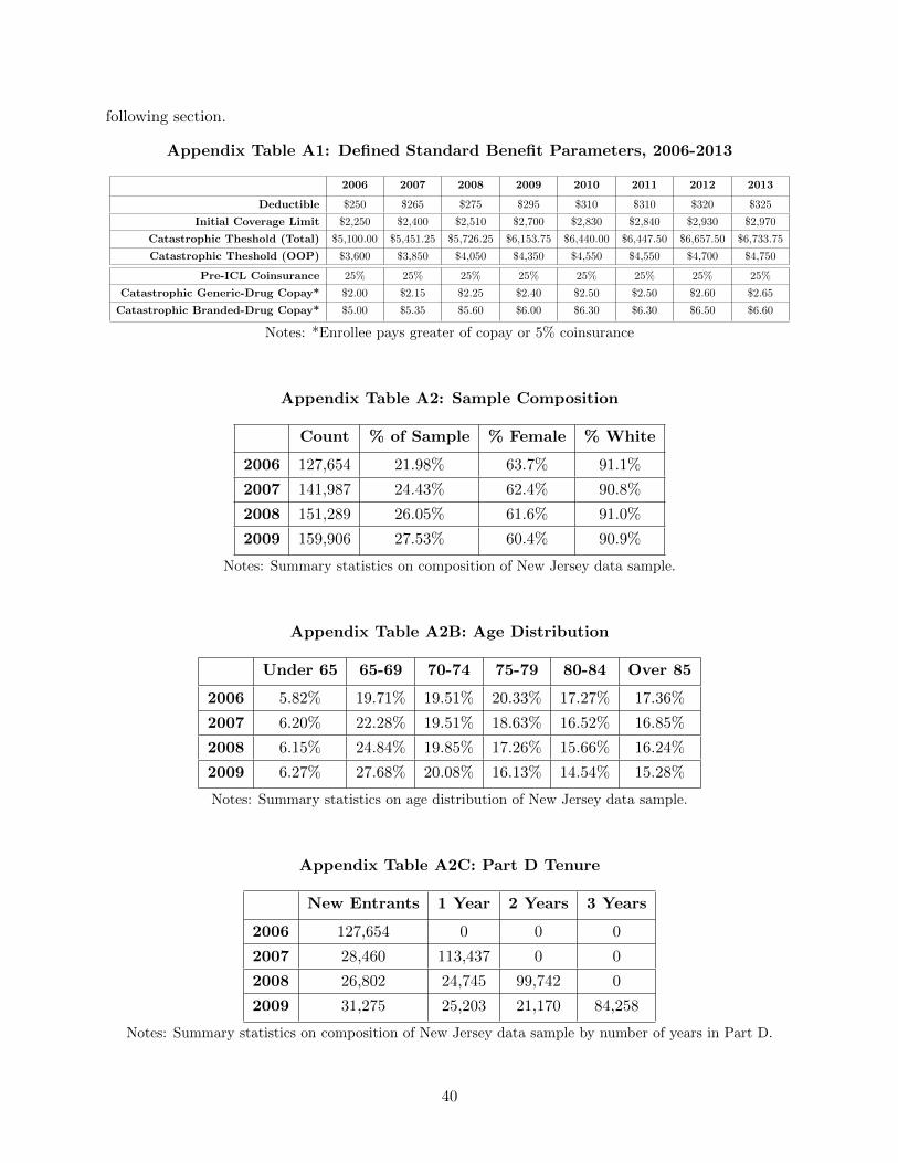
following section.
Appendix Table A1: Defined Standard Benefit Parameters, 2006-2013
2006 2007 2008 2009 2010 2011 2012 2013
Deductible $250 $265 $275 $295 $310 $310 $320 $325
Initial Coverage Limit $2,250 $2,400 $2,510 $2,700 $2,830 $2,840 $2,930 $2,970
Catastrophic Theshold (Total) $5,100.00 $5,451.25 $5,726.25 $6,153.75 $6,440.00 $6,447.50 $6,657.50 $6,733.75
Catastrophic Theshold (OOP) $3,600 $3,850 $4,050 $4,350 $4,550 $4,550 $4,700 $4,750
Pre-ICL Coinsurance 25% 25% 25% 25% 25% 25% 25% 25%
Catastrophic Generic-Drug Copay* $2.00 $2.15 $2.25 $2.40 $2.50 $2.50 $2.60 $2.65
Catastrophic Branded-Drug Copay* $5.00 $5.35 $5.60 $6.00 $6.30 $6.30 $6.50 $6.60
Notes: *Enrollee pays greater of copay or 5% coinsurance
Appendix Table A2: Sample Composition
Count % of Sample % Female % White
2006 127,654 21.98% 63.7% 91.1%
2007 141,987 24.43% 62.4% 90.8%
2008 151,289 26.05% 61.6% 91.0%
2009 159,906 27.53% 60.4% 90.9%
Notes: Summary statistics on composition of New Jersey data sample.
Appendix Table A2B: Age Distribution
Under 65 65-69 70-74 75-79 80-84 Over 85
2006 5.82% 19.71% 19.51% 20.33% 17.27% 17.36%
2007 6.20% 22.28% 19.51% 18.63% 16.52% 16.85%
2008 6.15% 24.84% 19.85% 17.26% 15.66% 16.24%
2009 6.27% 27.68% 20.08% 16.13% 14.54% 15.28%
Notes: Summary statistics on age distribution of New Jersey data sample.
Appendix Table A2C: Part D Tenure
New Entrants 1 Year 2 Years 3 Years
2006 127,654 0 0 0
2007 28,460 113,437 0 0
2008 26,802 24,745 99,742 0
2009 31,275 25,203 21,170 84,258
Notes: Summary statistics on composition of New Jersey data sample by number of years in Part D.
40
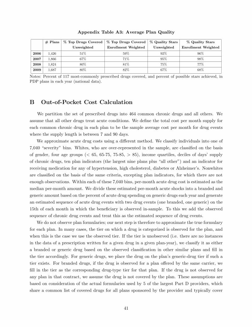
Appendix Table A3: Average Plan Quality
# Plans % Top Drugs Covered % Top Drugs Covered % Quality Stars % Quality Stars
Unweighted Enrollment Weighted Unweighted Enrollment Weighted
2006 1,426 51% 59% 92% 96%
2007 1,866 67% 71% 95% 98%
2008 1,824 80% 81% 75% 77%
2009 1,687 80% 82% 67% 68%
Notes: Percent of 117 most-commonly prescribed drugs covered, and percent of possible stars achieved, inPDP plans in each year (national data).
B Out-of-Pocket Cost Calculation
We partition the set of prescribed drugs into 464 common chronic drugs and all others. We
assume that all other drugs treat acute conditions. We define the total cost per month supply for
each common chronic drug in each plan to be the sample average cost per month for drug events
where the supply length is between 7 and 90 days.
We approximate acute drug costs using a different method. We classify individuals into one of
7,040 “severity” bins. Whites, who are over-represented in the sample, are classified on the basis
of gender, four age groups (< 65, 65-75, 75-85, > 85), income quartiles, deciles of days’ supply
of chronic drugs, ten plan indicators (the largest nine plans plus “all other”) and an indicator for
receiving medication for any of hypertension, high cholesterol, diabetes or Alzheimer’s. Nonwhites
are classified on the basis of the same criteria, excepting plan indicators, for which there are not
enough observations. Within each of these 7,040 bins, per-month acute drug cost is estimated as the
median per-month amount. We divide these estimated per-month acute shocks into a branded and
generic amount based on the percent of acute drug spending on generic drugs each year and generate
an estimated sequence of acute drug events with two drug events (one branded, one generic) on the
15th of each month in which the beneficiary is observed in-sample. To this we add the observed
sequence of chronic drug events and treat this as the estimated sequence of drug events.
We do not observe plan formularies; our next step is therefore to approximate the true formulary
for each plan. In many cases, the tier on which a drug is categorized is observed for the plan, and
when this is the case we use the observed tier. If the tier is unobserved (i.e. there are no instances
in the data of a prescription written for a given drug in a given plan-year), we classify it as either
a branded or generic drug based on the observed classification in other similar plans and fill in
the tier accordingly. For generic drugs, we place the drug on the plan’s generic-drug tier if such a
tier exists. For branded drugs, if the drug is observed for a plan offered by the same carrier, we
fill in the tier as the corresponding drug-type tier for that plan. If the drug is not observed for
any plan in that contract, we assume the drug is not covered by the plan. These assumptions are
based on consideration of the actual formularies used by 5 of the largest Part D providers, which
share a common list of covered drugs for all plans sponsored by the provider and typically cover
41

any generic drug but not all branded drugs. For simplicity we assume that the Pre-Initial Coverage
Limit and Gap phases employ the same formulary structure, as they do for the few plans with Gap
tiers, and we ignore the effect of specialty tiers as only one of the 464 most-commonly prescribed
chronic drugs is a specialty treatment.
Finally, to generate counterfactual spending under each plan we step through the simulated
sequence of drug events and generate counterfactual benefit phases and patient OOP payments
according to the plan’s stated cost structure, the estimated formulary, and cumulative spending
for the year. Counterfactual OOP payments for each plan are estimated as the sum of OOP
payments for the observed chronic drugs and simulated acute events for each beneficiary in each
large plan every year. Note that, as in previous papers, our method assumes no moral hazard, and
unlike Ketcham et al. (2012) we assume no elasticity with respect to plan prices for chronic drug
consumption, in that patients take the same sequence of prescription drugs in every plan regardless
of the costs they face. The plan-specific medians allow for some price elasticity for acute drugs for
large plans. For simplicity we ignore the effect of prior authorization requirement, step therapy
regimens and quantity restrictions.
The estimated payments, which represent the “True Out-of-Pocket Payments”, are added to
a premium payment for each month in which the beneficiary is enrolled in the plan to create a
counterfactual “Total Payment” variable for each beneficiary in each plan. These numbers are
scaled up to a 12-month equivalent for each beneficiary enrolled for fewer than 12 months. The
minimum cost plan for each beneficiary is defined as the plan with lowest “Total Payment” in each
year.
C Analyzing the Empirical Behavior of Part D Enrollees
We investigate of the behavior of Part D enrollees by considering the amount they pay in
their chosen plan given the costs of the other plans that are available to them. We refer to the gap
between what the consumer spent and the lowest cost plan she could have chosen as “overspending”
or gap spending. Table 1 in the text shows overspending relative to the minimum cost plan by
Part D cohort. These numbers indicate that there is variation across cohorts, particularly between
new enrollees and those with experience of the program. New enrollees’ spending gap was lower in
2008 and 2009 than that of continuing enrollees, reaching a level of $371.78 or 32% in 2009. 2006
enrollees (those who first entered the program in 2006 and remained in it throughout our sample)
had above-average gaps in every year relative to the full sample; their level of spending above the
lowest cost plan in 2009 was $459.19, or roughly the same percentage of total cost (37%) as in 2006
despite their long exposure to the program.
Part of the spending gap shown by Part D enrollees is a result of failing to choose a new plan
each year. Column 1 of Table C2 shows that in every year, consistent with Ketcham et al. (2012),
the spending gap is on average lower for consumers who have just switched plans. Moreover, the
spending gap for the group switching decreases slightly over time, while that for non-switchers
42

Appendix Table C1: Switching by Demographic Group
2006-07 2007-08 2008-09
Whole Sample 19.08% 24.07% 8.16%
Female 20.86% 26.27% 8.54%
Non-White 21.68% 26.94% 8.83%
Income 2006-07 2007-08 2008-09
1st Quartile (low) 24.84% 30.60% 9.00%
2nd Quartile 19.84% 24.76% 8.18%
3rd Quartile 18.01% 23.20% 8.22%
4th Quartile (high) 13.99% 18.49% 7.43%
Age 2006-07 2007-08 2008-09
Under 65 29.28% 33.23% 11.32%
65-69 12.78% 18.08% 7.68%
70-74 14.71% 20.03% 7.55%
75-79 17.03% 22.33% 7.55%
80-84 20.65% 25.20% 7.64%
Over 85 27.45% 33.37% 9.80%
Notes: Percent of enrollees switching plans in NJ data, by year and demographic group.
Table C2: Spending Gap by Switch Decision
% Error, Next- % Error, Next- ∆% Error, ∆% Error, ∆% Error, ChosenSwitchers Year Chosen Plan Year Same Plan Chosen Plan Same Plan Relative to Same
2006 27.97% 35.01% -16.66% -9.62% -7.04%
2007 28.09% 42.98% 2.35% 17.24% -14.89%
2008 25.83% 39.75% -4.12% 9.80% -13.92%
% Error, Next- % Error, Next- ∆% Error, ∆% Error, ∆% Error, ChosenNon-Switchers Year Chosen Plan Year Same Plan Chosen Plan Same Plan Relative to Same
2006 29.81% 29.81% -5.55% -5.55% 0.00%
2007 35.00% 35.00% 4.07% 4.07% 0.00%
2008 37.07% 37.07% 6.03% 6.03% 0.00%
Notes: Predicted percent error in observed chosen plan, and under scenario where enrollee stays in previous-year plan, for both switchers and non-switchers.
43
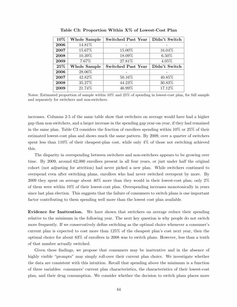
Table C3: Proportion Within X% of Lowest-Cost Plan
10% Whole Sample Switched Past Year Didn’t Switch
2006 14.81% - -
2007 15.67% 15.00% 16.04%
2008 10.39% 18.09% 6.50%
2009 7.67% 27.81% 4.05%
25% Whole Sample Switched Past Year Didn’t Switch
2006 28.06% - -
2007 42.82% 50.16% 40.85%
2008 35.27% 44.23% 30.83%
2009 21.74% 46.99% 17.12%
Notes: Estimated proportion of sample within 10% and 25% of spending in lowest-cost plan, for full sampleand separately for switchers and non-switchers.
increases. Columns 2-5 of the same table show that switchers on average would have had a higher
gap than non-switchers, and a larger increase in the spending gap year-on-year, if they had remained
in the same plan. Table C3 considers the fraction of enrollees spending within 10% or 25% of their
estimated lowest-cost plan and shows much the same pattern. By 2009, over a quarter of switchers
spent less than 110% of their cheapest-plan cost, while only 4% of those not switching achieved
this.
The disparity in overspending between switchers and non-switchers appears to be growing over
time. By 2009, around 62,000 enrollees present in all four years, or just under half the original
cohort (not adjusting for attrition) had never picked a new plan. While switchers continued to
overspend even after switching plans, enrollees who had never switched overspent by more. By
2009 they spent on average about 40% more than they would in their lowest-cost plan; only 2%
of them were within 10% of their lowest-cost plan. Overspending increases monotonically in years
since last plan election. This suggests that the failure of consumers to switch plans is one important
factor contributing to them spending well more than the lowest cost plan available.
Evidence for Inattention. We have shown that switchers on average reduce their spending
relative to the minimum in the following year. The next key question is why people do not switch
more frequently. If we conservatively define switching as the optimal choice whenever a consumer’s
current plan is expected to cost more than 125% of the cheapest plan’s cost next year, then the
optimal choice for about 83% of enrollees in 2008 was to switch plans. However, less than a tenth
of that number actually switched.
Given these findings, we propose that consumers may be inattentive and in the absence of
highly visible “prompts” may simply roll-over their current plan choice. We investigate whether
the data are consistent with this intuition. Recall that spending above the minimum is a function
of three variables: consumers’ current plan characteristics, the characteristics of their lowest-cost
plan, and their drug consumption. We consider whether the decision to switch plans places more
44

weight on own-plan and personal characteristics, which are readily observable, than on optimal-plan
characteristics, which require costly search.
We construct three simple indicators for “shocks” to expected spending that depend only own-
plan and personal characteristics. We define a “premium shock” as an increase in own-plan premi-
ums the following year of greater than the weighted median increase across all consumers (about
$4 in 2007, $7 in 2008, and $4.50 in 2009).41 Each year in the open enrollment period an existing
enrollee receives a letter from his or her plan detailing changes in the coming year. To the extent
the enrollee opens the letter and reads it, the premium increase becomes known and salient at a
time when the enrollee can easily switch plans. A “coverage shock” is defined as occurring when
either (a) the consumer’s current plan drops coverage in the coverage gap or (b) the plan moves
from the defined standard benefit pre-ICL (before hitting the coverage gap) to a tiered system
in that region.42 Third, we define enrollees as receiving an “acute shock” if they are in the top
quintile of total spending and also the top decile for either percent spending on acute drugs or
deviation between predicted and observed spending in the current year. This shock is meant to
capture unanticipated short-term illness, which may prompt the consumer to scrutinize her choice
of insurance while also serving as signal of high expected future spending.43
Table C4 shows the results of probit regressions of decision to switch plans on own-plan, low-
cost plan and personal characteristics. If consumers prefer low premiums and high coverage but
are inattentive, we expect them to switch more frequently when their current plan raises premium
or reduces coverage than when other low-cost plans reduce premium or increase coverage. If they
switch in response to acute shocks we expect those with high OOP spending to switch. The
estimates in Table C4 are consistent with this intuition. In all specifications enrollees with high
OOP spending and those with high premiums and deductibles and without gap coverage switch
more than other consumers. Model 1 indicates that consumers’ switching probability increases
when their own plan’s premium rises or when their own plan removes gap coverage. Model 2 adds
the equivalent variables for the average of the five lowest-cost plans and shows that, to the extent
changes in other-plan characteristics affect switching at all, the correlations run in the “wrong”
direction. In particular it seems that consumers are more likely to switch when low-cost plans
increase their premiums. Changes in low-cost plans’ gap coverage have no significant effect44.
Table C5 presents evidence that consumers who switch select plans with characteristics that
vary depending on the shock that prompted the switch. Consumers who receive acute shocks,
41We have experimented with different cutoffs and the median does well in terms of simplicity and explanatorypower.
42Recall that basic plans must meet a coverage standard and be actuarially equivalent to the tariff set out in thelaw. The declines we label as “shocks” are declines in one part of the benefit schedule, which we treat as appropriatemeasures of rapidly increasing premiums and eroding (or increasingly complex) coverage on some dimension. Wecould also potentially have considered other shock definitions such as pharmacy network changes, or indicators forindividual enrollees’ preferred drugs being dropped. Unfortunately the data were not ideal for these definitions.
43We do not have information on diagnoses because we only have data from Medicare Part D and not Parts Aand B. However, a diagnosis - and in particular an inferred diagnosis - may be a less precise measure of how muchpharmaceutical spending increases compared to actual utilization.
44The results are insensitive to using either the lowest-cost plan available, the lowest-cost plan within-brand, or anaverage of the 5 lowest-cost plans.
45
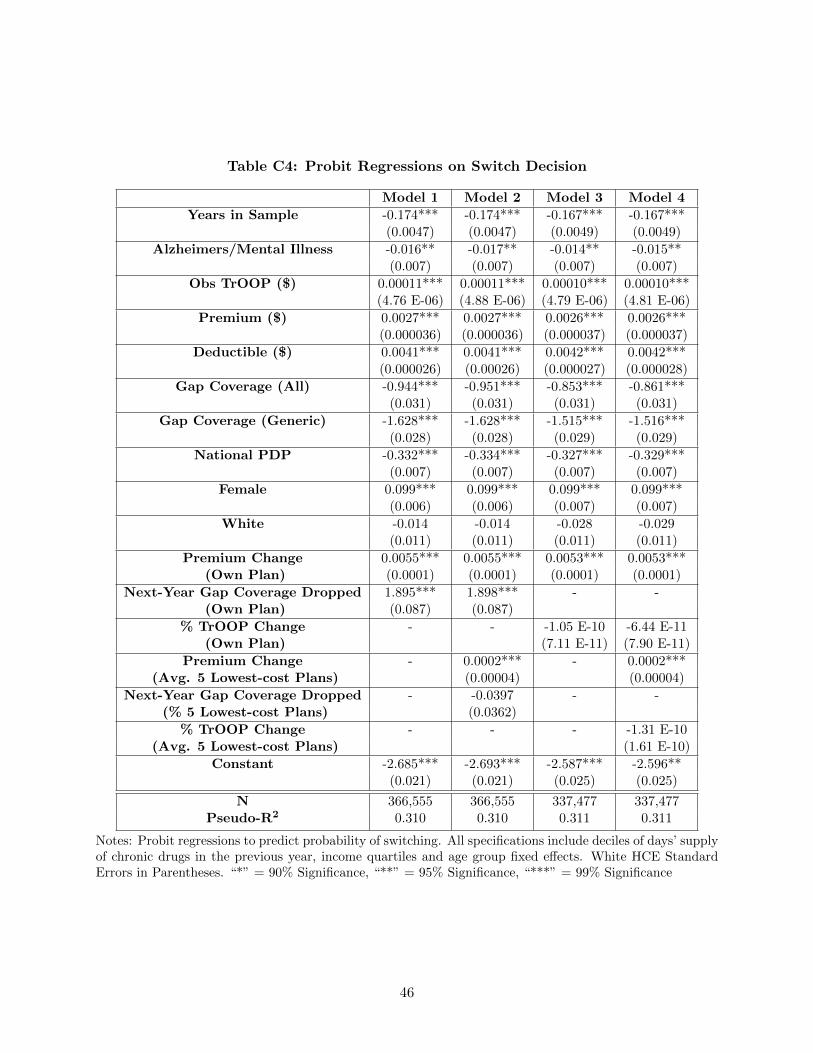
Table C4: Probit Regressions on Switch Decision
Model 1 Model 2 Model 3 Model 4
Years in Sample -0.174*** -0.174*** -0.167*** -0.167***(0.0047) (0.0047) (0.0049) (0.0049)
Alzheimers/Mental Illness -0.016** -0.017** -0.014** -0.015**(0.007) (0.007) (0.007) (0.007)
Obs TrOOP ($) 0.00011*** 0.00011*** 0.00010*** 0.00010***(4.76 E-06) (4.88 E-06) (4.79 E-06) (4.81 E-06)
Premium ($) 0.0027*** 0.0027*** 0.0026*** 0.0026***(0.000036) (0.000036) (0.000037) (0.000037)
Deductible ($) 0.0041*** 0.0041*** 0.0042*** 0.0042***(0.000026) (0.00026) (0.000027) (0.000028)
Gap Coverage (All) -0.944*** -0.951*** -0.853*** -0.861***(0.031) (0.031) (0.031) (0.031)
Gap Coverage (Generic) -1.628*** -1.628*** -1.515*** -1.516***(0.028) (0.028) (0.029) (0.029)
National PDP -0.332*** -0.334*** -0.327*** -0.329***(0.007) (0.007) (0.007) (0.007)
Female 0.099*** 0.099*** 0.099*** 0.099***(0.006) (0.006) (0.007) (0.007)
White -0.014 -0.014 -0.028 -0.029(0.011) (0.011) (0.011) (0.011)
Premium Change 0.0055*** 0.0055*** 0.0053*** 0.0053***(Own Plan) (0.0001) (0.0001) (0.0001) (0.0001)
Next-Year Gap Coverage Dropped 1.895*** 1.898*** - -(Own Plan) (0.087) (0.087)
% TrOOP Change - - -1.05 E-10 -6.44 E-11(Own Plan) (7.11 E-11) (7.90 E-11)
Premium Change - 0.0002*** - 0.0002***(Avg. 5 Lowest-cost Plans) (0.00004) (0.00004)
Next-Year Gap Coverage Dropped - -0.0397 - -(% 5 Lowest-cost Plans) (0.0362)
% TrOOP Change - - - -1.31 E-10(Avg. 5 Lowest-cost Plans) (1.61 E-10)
Constant -2.685*** -2.693*** -2.587*** -2.596**(0.021) (0.021) (0.025) (0.025)
N 366,555 366,555 337,477 337,477Pseudo-R2 0.310 0.310 0.311 0.311
Notes: Probit regressions to predict probability of switching. All specifications include deciles of days’ supplyof chronic drugs in the previous year, income quartiles and age group fixed effects. White HCE StandardErrors in Parentheses. “*” = 90% Significance, “**” = 95% Significance, “***” = 99% Significance
46

which we can think of as signals of future ill-health, tend to prefer higher coverage conditional on
switching than those who do not. The same is true of those receiving coverage shocks. Consumers
facing premium shocks tend to choose plans with lower premiums. This suggests that consumers
treat shocks to their health status and plan characteristics not only as prompts to switch but also
as “cues” to search for particular plan attributes, as in Busse et al. (2014).
Table C5: Next-Year Plan Choices and Overspending by Shock, Switchers Only
2006 Acute Shock No Acute Premium Shock No Premium Cov Shock No Cov
% Gap Coverage 14.10% 7.13% 3.46% 45.41% 30.87% 5.95%
Premium 20.83 18.82 17.46 32.47 29.65 18.16
% within 25% 72.07% 49.55% 52.29% 47.98% 62.53% 50.96%
2007 Acute Shock No Acute Premium Shock No Premium Cov Shock No Cov
% Gap Coverage 5.39% 3.20% 2.97% 5.29% 0.00% 3.41%
Premium 27.25 26.43 25.77 29.68 22.10 26.50
% within 25% 64.99% 42.20% 46.70% 34.20% 0,00% 44.37%
2008 Acute Shock No Acute Premium Shock No Premium Cov Shock No Cov
% Gap Coverage 9.54% 4.34% 3.55% 9.12% 2.44% 4.98%
Premium 31.84 29.76 29.07 32.97 29.99 29.92
% within 25% 58.28% 46.56% 47.91% 46.18% 46.45% 47.63%
Overall Acute Shock No Acute Premium Shock No Premium Cov Shock No Cov
% Gap Coverage 9.23% 4.75% 3.25% 15.08% 21.07% 4.52%
Premium 25.54 24.36 23.19 31.05 29.76 24.26
% within 25% 66.63% 45.49% 48.98% 39.98% 56.97% 47.11%
N 5,924 56,183 51,955 10,152 2, 496 59,611
Notes: Summary of types of plans chosen by type of shock experienced. ‘% Gap Coverage’ is average percentof plans chosen with gap coverage; ’Premium” is average premium per enrollee per month for chosen plan;‘% within 25%’ is percent of plans chosen that are within 25% of lowest-cost option available.
Alternative Explanations. There is a significant insurance literature that examines the ques-
tion of risk-aversion and whether consumers over-insure themselves because they have great distaste
for risk. This might be an explanation of our initial findings, and those of other Part D papers.
However, in our data we do not find evidence to support this theory – that high spending by non-
switchers is related to over-insurance, as would be the case if risk aversion was causing the observed
overspending. Appendix Table C6 shows that the percentage of enrollees’ total costs covered in the
gap is much higher for switchers than for non-switchers, while premiums are on average lower for
switchers. Thus higher coverage is chosen by people who overspend by less, rather than more, on
average. In addition, this increased gap coverage does not come at the expense of reduced coverage
in the pre-ICL phase (the main coverage phase), as the percent of covered costs isactually higher
in this phase on average for switchers as well. Note that the coverage figures in Appendix Table
C6 summarize the percent of costs covered for consumers enrolled in the relevant plan, not for the
statistical average enrollee used for the CMS actuarial equivalence calculations.
47

Appendix Table C6: Following-Year Plan Characteristics Choices, Switchers and NonSwitchers
Switchers % Enhanced Premium % Pre-ICL Cvge % ICL Cvge
2006 14.64% 19.02 70.15% 12.15%
2007 24.00% 26.50 70.50% 29.29%
2008 37.53% 29.93 71.34% 29.60%
Non Switchers % Enhanced Premium % Pre-ICL Cvge % ICL Cvge
2006 28.13% 26.02 62.29% 10.29%
2007 33.62% 38.63 65.85% 6.52%
2008 31.58% 38.31 62.40% 9.07%
Notes: Comparison of observed plan characteristics, for switchers and non-switchers. ‘% Pre-ICL Cvge’ isaverage observed percent of costs covered by the plan in Pre-ICL phase for that plan’s enrollees; ‘% ICLCvge’ is analogous figure for costs in the coverage gap.
We also run cross-sectional regressions of percent overspending, defined as the difference be-
tween the chosen and minimum cost plans divided by the chosen plan’s cost, on plan and enrollee
characteristics. The results are set out in Appendix Table C7. Having switched plans is negatively
and significantly related to overspending, and whether or not we control for having switched plans,
gap coverage is negatively related, and premiums and deductibles positively related to overspending
conditional on observed OOP costs. Therefore we conclude that overspending is not on average
associated with overinsurance in our data.
A second possible explanation for overspending is that it takes experience to learn how to shop
in the Part D marketplace. Perhaps an enrollee’s overspending falls over time as she learns. Table
1 in the text addresses this issue. 2006 enrollees - those who first entered the program in 2006 and
remained in it throughout our sample - had higher overspending in every year than the average for
the full sample; their overspending in 2009 was $459.19, or roughly the same percentage of total
cost (37%) as in 2006 despite their long exposure to the program. This suggests that overspending
is not declining with experience in Part D.
48
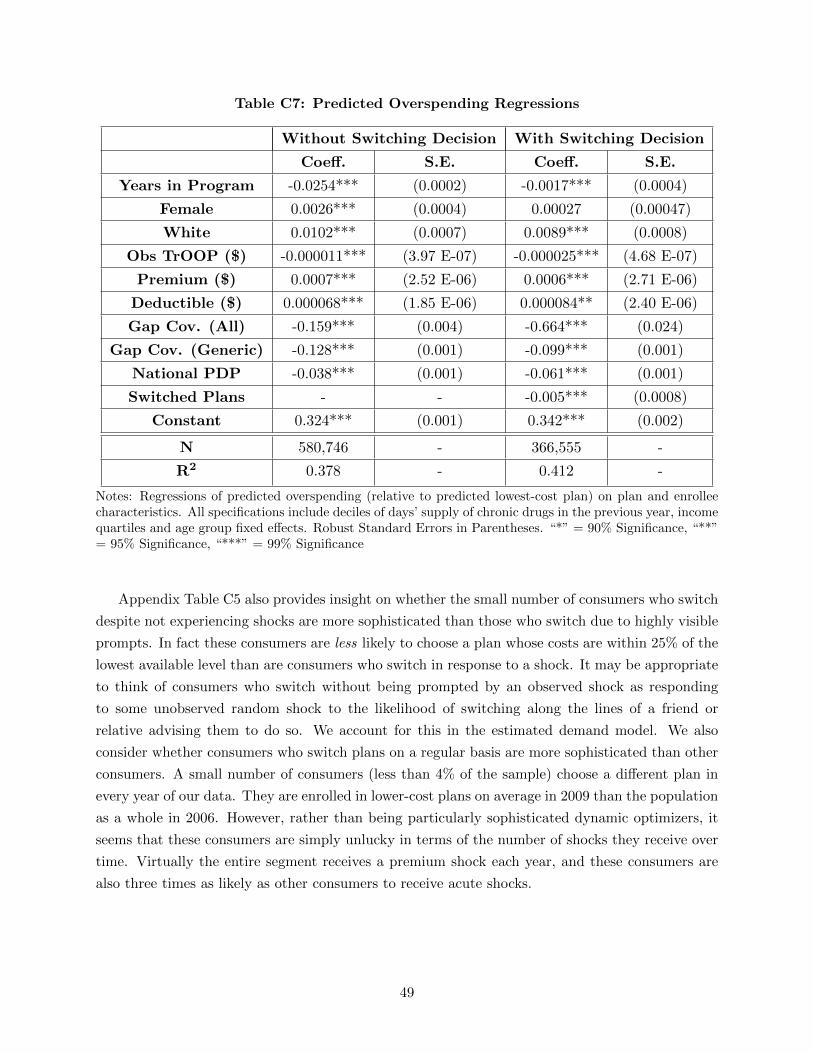
Table C7: Predicted Overspending Regressions
Without Switching Decision With Switching Decision
Coeff. S.E. Coeff. S.E.
Years in Program -0.0254*** (0.0002) -0.0017*** (0.0004)
Female 0.0026*** (0.0004) 0.00027 (0.00047)
White 0.0102*** (0.0007) 0.0089*** (0.0008)
Obs TrOOP ($) -0.000011*** (3.97 E-07) -0.000025*** (4.68 E-07)
Premium ($) 0.0007*** (2.52 E-06) 0.0006*** (2.71 E-06)
Deductible ($) 0.000068*** (1.85 E-06) 0.000084** (2.40 E-06)
Gap Cov. (All) -0.159*** (0.004) -0.664*** (0.024)
Gap Cov. (Generic) -0.128*** (0.001) -0.099*** (0.001)
National PDP -0.038*** (0.001) -0.061*** (0.001)
Switched Plans - - -0.005*** (0.0008)
Constant 0.324*** (0.001) 0.342*** (0.002)
N 580,746 - 366,555 -
R2 0.378 - 0.412 -
Notes: Regressions of predicted overspending (relative to predicted lowest-cost plan) on plan and enrolleecharacteristics. All specifications include deciles of days’ supply of chronic drugs in the previous year, incomequartiles and age group fixed effects. Robust Standard Errors in Parentheses. “*” = 90% Significance, “**”= 95% Significance, “***” = 99% Significance
Appendix Table C5 also provides insight on whether the small number of consumers who switch
despite not experiencing shocks are more sophisticated than those who switch due to highly visible
prompts. In fact these consumers are less likely to choose a plan whose costs are within 25% of the
lowest available level than are consumers who switch in response to a shock. It may be appropriate
to think of consumers who switch without being prompted by an observed shock as responding
to some unobserved random shock to the likelihood of switching along the lines of a friend or
relative advising them to do so. We account for this in the estimated demand model. We also
consider whether consumers who switch plans on a regular basis are more sophisticated than other
consumers. A small number of consumers (less than 4% of the sample) choose a different plan in
every year of our data. They are enrolled in lower-cost plans on average in 2009 than the population
as a whole in 2006. However, rather than being particularly sophisticated dynamic optimizers, it
seems that these consumers are simply unlucky in terms of the number of shocks they receive over
time. Virtually the entire segment receives a premium shock each year, and these consumers are
also three times as likely as other consumers to receive acute shocks.
49
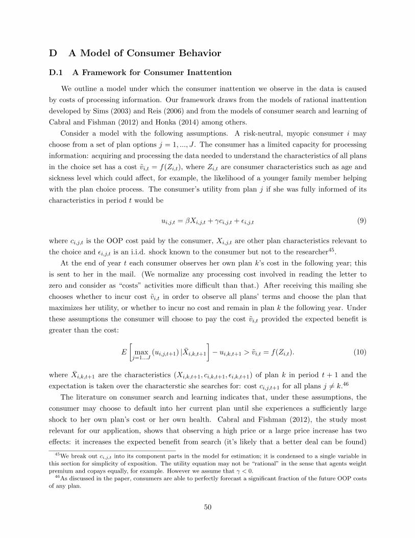
D A Model of Consumer Behavior
D.1 A Framework for Consumer Inattention
We outline a model under which the consumer inattention we observe in the data is caused
by costs of processing information. Our framework draws from the models of rational inattention
developed by Sims (2003) and Reis (2006) and from the models of consumer search and learning of
Cabral and Fishman (2012) and Honka (2014) among others.
Consider a model with the following assumptions. A risk-neutral, myopic consumer i may
choose from a set of plan options j = 1, ..., J . The consumer has a limited capacity for processing
information: acquiring and processing the data needed to understand the characteristics of all plans
in the choice set has a cost vi,t = f(Zi,t), where Zi,t are consumer characteristics such as age and
sickness level which could affect, for example, the likelihood of a younger family member helping
with the plan choice process. The consumer’s utility from plan j if she was fully informed of its
characteristics in period t would be
ui,j,t = βXi,j,t + γci,j,t + εi,j,t (9)
where ci,j,t is the OOP cost paid by the consumer, Xi,j,t are other plan characteristics relevant to
the choice and εi,j,t is an i.i.d. shock known to the consumer but not to the researcher45.
At the end of year t each consumer observes her own plan k’s cost in the following year; this
is sent to her in the mail. (We normalize any processing cost involved in reading the letter to
zero and consider as “costs” activities more difficult than that.) After receiving this mailing she
chooses whether to incur cost vi,t in order to observe all plans’ terms and choose the plan that
maximizes her utility, or whether to incur no cost and remain in plan k the following year. Under
these assumptions the consumer will choose to pay the cost vi,t provided the expected benefit is
greater than the cost:
E
[maxj=1...J
(ui,j,t+1) |Xi,k,t+1
]− ui,k,t+1 > vi,t = f(Zi,t). (10)
where Xi,k,t+1 are the characteristics (Xi,k,t+1, ci,k,t+1, εi,k,t+1) of plan k in period t + 1 and the
expectation is taken over the characterstic she searches for: cost ci,j,t+1 for all plans j 6= k.46
The literature on consumer search and learning indicates that, under these assumptions, the
consumer may choose to default into her current plan until she experiences a sufficiently large
shock to her own plan’s cost or her own health. Cabral and Fishman (2012), the study most
relevant for our application, shows that observing a high price or a large price increase has two
effects: it increases the expected benefit from search (it’s likely that a better deal can be found)
45We break out ci,j,t into its component parts in the model for estimation; it is condensed to a single variable inthis section for simplicity of exposition. The utility equation may not be “rational” in the sense that agents weightpremium and copays equally, for example. However we assume that γ < 0.
46As discussed in the paper, consumers are able to perfectly forecast a significant fraction of the future OOP costsof any plan.
50
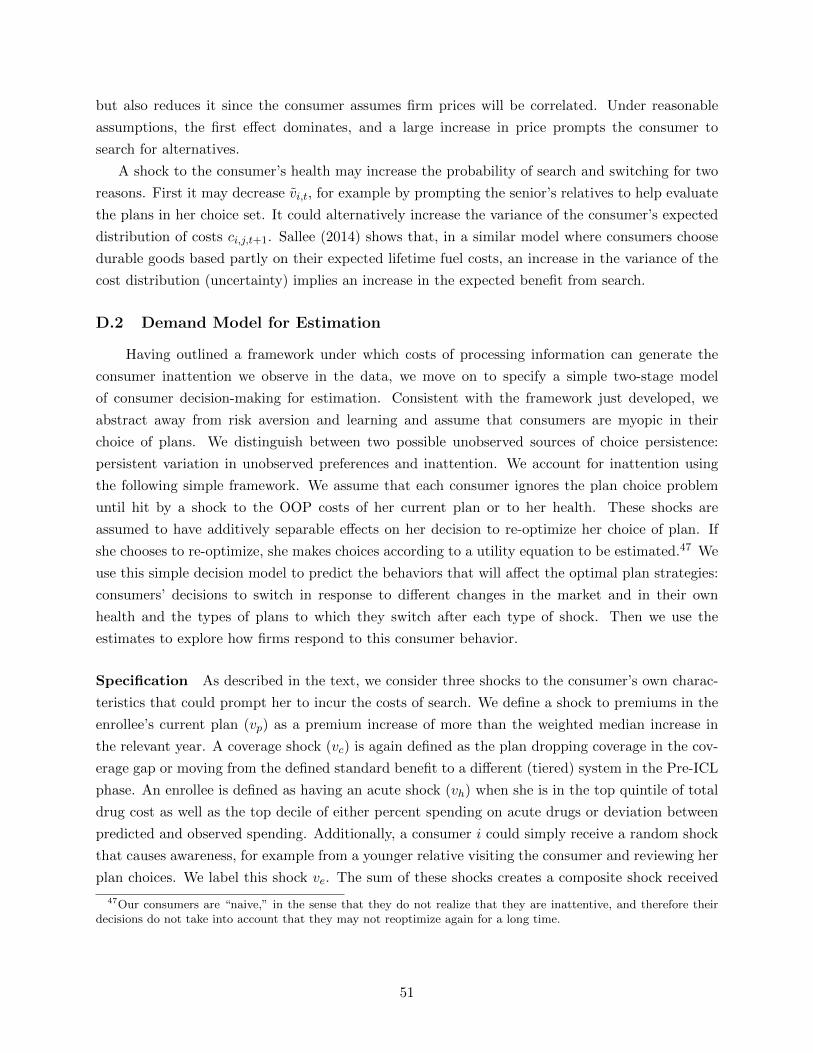
but also reduces it since the consumer assumes firm prices will be correlated. Under reasonable
assumptions, the first effect dominates, and a large increase in price prompts the consumer to
search for alternatives.
A shock to the consumer’s health may increase the probability of search and switching for two
reasons. First it may decrease vi,t, for example by prompting the senior’s relatives to help evaluate
the plans in her choice set. It could alternatively increase the variance of the consumer’s expected
distribution of costs ci,j,t+1. Sallee (2014) shows that, in a similar model where consumers choose
durable goods based partly on their expected lifetime fuel costs, an increase in the variance of the
cost distribution (uncertainty) implies an increase in the expected benefit from search.
D.2 Demand Model for Estimation
Having outlined a framework under which costs of processing information can generate the
consumer inattention we observe in the data, we move on to specify a simple two-stage model
of consumer decision-making for estimation. Consistent with the framework just developed, we
abstract away from risk aversion and learning and assume that consumers are myopic in their
choice of plans. We distinguish between two possible unobserved sources of choice persistence:
persistent variation in unobserved preferences and inattention. We account for inattention using
the following simple framework. We assume that each consumer ignores the plan choice problem
until hit by a shock to the OOP costs of her current plan or to her health. These shocks are
assumed to have additively separable effects on her decision to re-optimize her choice of plan. If
she chooses to re-optimize, she makes choices according to a utility equation to be estimated.47 We
use this simple decision model to predict the behaviors that will affect the optimal plan strategies:
consumers’ decisions to switch in response to different changes in the market and in their own
health and the types of plans to which they switch after each type of shock. Then we use the
estimates to explore how firms respond to this consumer behavior.
Specification As described in the text, we consider three shocks to the consumer’s own charac-
teristics that could prompt her to incur the costs of search. We define a shock to premiums in the
enrollee’s current plan (vp) as a premium increase of more than the weighted median increase in
the relevant year. A coverage shock (vc) is again defined as the plan dropping coverage in the cov-
erage gap or moving from the defined standard benefit to a different (tiered) system in the Pre-ICL
phase. An enrollee is defined as having an acute shock (vh) when she is in the top quintile of total
drug cost as well as the top decile of either percent spending on acute drugs or deviation between
predicted and observed spending. Additionally, a consumer i could simply receive a random shock
that causes awareness, for example from a younger relative visiting the consumer and reviewing her
plan choices. We label this shock ve. The sum of these shocks creates a composite shock received
47Our consumers are “naive,” in the sense that they do not realize that they are inattentive, and therefore theirdecisions do not take into account that they may not reoptimize again for a long time.
51
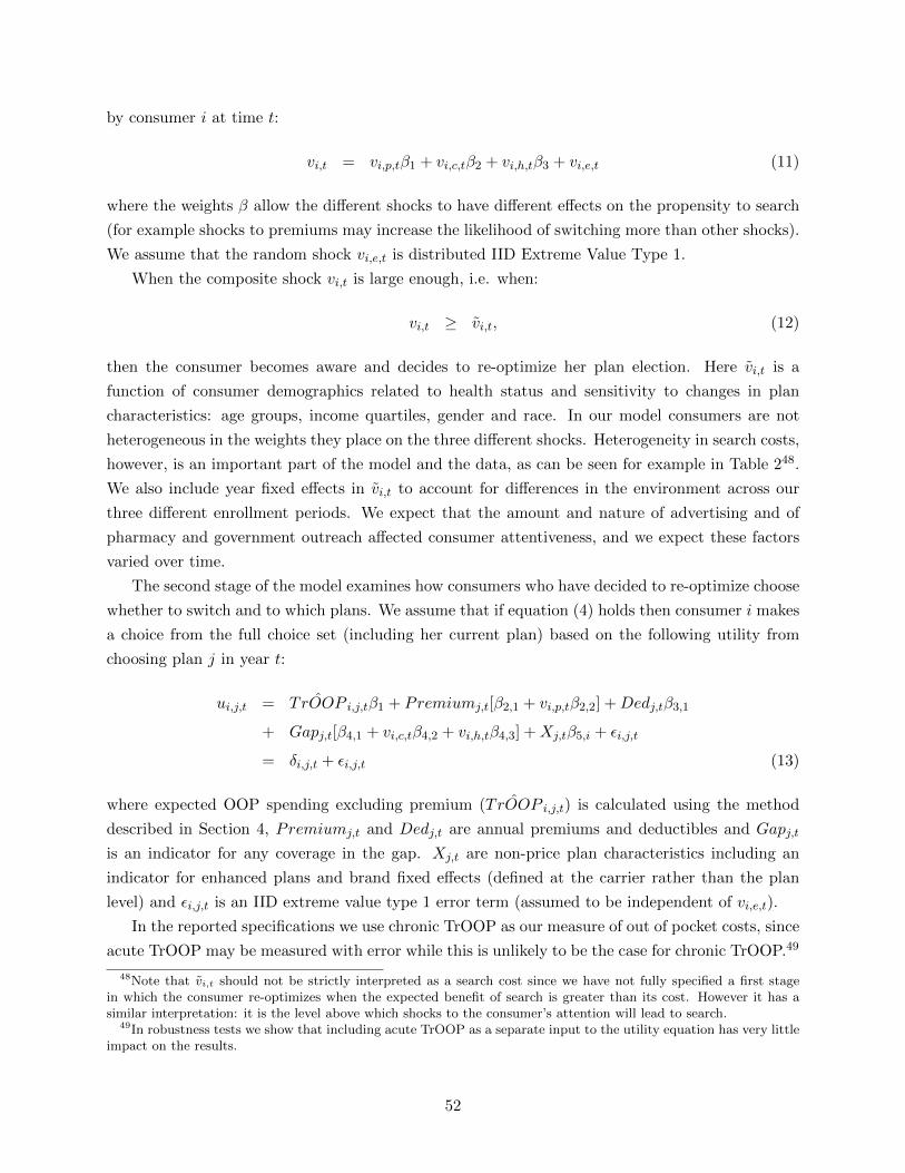
by consumer i at time t:
vi,t = vi,p,tβ1 + vi,c,tβ2 + vi,h,tβ3 + vi,e,t (11)
where the weights β allow the different shocks to have different effects on the propensity to search
(for example shocks to premiums may increase the likelihood of switching more than other shocks).
We assume that the random shock vi,e,t is distributed IID Extreme Value Type 1.
When the composite shock vi,t is large enough, i.e. when:
vi,t ≥ vi,t, (12)
then the consumer becomes aware and decides to re-optimize her plan election. Here vi,t is a
function of consumer demographics related to health status and sensitivity to changes in plan
characteristics: age groups, income quartiles, gender and race. In our model consumers are not
heterogeneous in the weights they place on the three different shocks. Heterogeneity in search costs,
however, is an important part of the model and the data, as can be seen for example in Table 248.
We also include year fixed effects in vi,t to account for differences in the environment across our
three different enrollment periods. We expect that the amount and nature of advertising and of
pharmacy and government outreach affected consumer attentiveness, and we expect these factors
varied over time.
The second stage of the model examines how consumers who have decided to re-optimize choose
whether to switch and to which plans. We assume that if equation (4) holds then consumer i makes
a choice from the full choice set (including her current plan) based on the following utility from
choosing plan j in year t:
ui,j,t = ˆTrOOP i,j,tβ1 + Premiumj,t[β2,1 + vi,p,tβ2,2] +Dedj,tβ3,1
+ Gapj,t[β4,1 + vi,c,tβ4,2 + vi,h,tβ4,3] +Xj,tβ5,i + εi,j,t
= δi,j,t + εi,j,t (13)
where expected OOP spending excluding premium ( ˆTrOOP i,j,t) is calculated using the method
described in Section 4, Premiumj,t and Dedj,t are annual premiums and deductibles and Gapj,t
is an indicator for any coverage in the gap. Xj,t are non-price plan characteristics including an
indicator for enhanced plans and brand fixed effects (defined at the carrier rather than the plan
level) and εi,j,t is an IID extreme value type 1 error term (assumed to be independent of vi,e,t).
In the reported specifications we use chronic TrOOP as our measure of out of pocket costs, since
acute TrOOP may be measured with error while this is unlikely to be the case for chronic TrOOP.49
48Note that vi,t should not be strictly interpreted as a search cost since we have not fully specified a first stagein which the consumer re-optimizes when the expected benefit of search is greater than its cost. However it has asimilar interpretation: it is the level above which shocks to the consumer’s attention will lead to search.
49In robustness tests we show that including acute TrOOP as a separate input to the utility equation has very littleimpact on the results.
52

Note that a consumer who could calculate expected costs perfectly would value a given change in
either TrOOP equally, and with the same weight as premium, as they are all measured in dollars.
We do not include a term for the variance of chronic TrOOP since consumers are assumed to predict
their chronic drug costs with certainty. While in principle a risk-neutral consumer should not put
any weight on other plan financial characteristics after correctly calculating TrOOP, we know from
past research that they do. Therefore we include other financial characteristics of the plan (the
size of the deductible and an indicator for coverage in the gap) in the utility equation to help us
predict consumer choice. Significant coefficients on these characteristics may reflect consumer risk
aversion, the salience of particular publicized plan characteristics, or other choice frictions that
we do not not formally model. In addition we allow consumers prompted to search by shocks to
premiums to place additional weight on premiums. Consumers experiencing shocks to coverage, or
acute shocks, are permitted to place additional weight on the plan offering gap coverage.
We model persistent unobserved preference heterogeneity by including normally-distributed
random coefficients β5,i on fixed effects for the three dominant brands, which together have over
80% market share in 2006, and on the enhanced plan fixed effect. The model therefore allows choice
persistence (such as a lack of switching away from a particular plan even when other plans reduce
their premiums) to be caused either by heterogeneous preferences (some consumers have a very
strong valuation for this brand that makes it worthwhile to remain enrolled even at a high relative
price) or by inattention (consumers who are not affected by any of the previously-defined shocks
are unaware of other plan premium reductions). One of our objectives in estimating this equation
is to distinguish between these two effects.50
The model is estimated using a random coefficients simulated maximum likelihood approach
similar to that summarized in Train (2009). Details are provided in the following subsection.
Identification The intuition for identification of this model is now fairly standard in the literature
(see for example Handel (2013) and Polyakova (2016)). We use the panel structure of the data,
which implies that we can track individuals making consecutive choices over several years, together
with the fact that new enrollees in the program enter the data in every year. These new enrollees are
assumed to choose without inertia; we also assume that the normally distributed random coefficients
fully capture the unobserved heterogeneity in their preferences. The parameters governing the
unobserved preference heterogeneity (the distribution of the random coefficients) can therefore
be estimated from the choices made by new enrollees in the program. Other determinants of
the decision to switch, most importantly the parameters governing inattention, are identified from
consumers’ observed sequences of choices in the years following entry. The initial conditions problem
50We choose not to model a third possible source of choice persistence: the existence of switching costs defined tobe distinct from the attention and search costs here. While switching costs has been a focus of some previous paperson health insurance markets (e.g. Handel (2013) and Polyakova (2016)), we find it difficult to separate out what thosemight be (time, effort, searching) and whether they overlap with the cognitive effort of paying attention to a particulardecision and investing in optimization. The evidence presented above indicates that inattention is an important sourceof search frictions in our data. We focus on identifying the effects of inattention separately from persistent unobservedpreferences, choosing not to attempt the notoriously difficult empirical task of also distinguishing between the effectsof asymmetric search costs (inattention) and switching costs.
53
(e.g., Heckman (1991)) does not arise in our data because we observe the first Part D choices for
all individuals in the estimation sample.
Endogeneity issues are of course also relevant for identification. A classic endogeneity problem
would occur if a plan’s additional coverage was valued in ways we did not observe and this additional
coverage was correlated with the plan’s premium. An insurer with an unobservably good plan that
wanted to charge a higher price could submit a higher bid to CMS and this would show up as a
higher premium. However, the institutional features of the Part D setting reduce this endogeneity
concern considerably. Because plans must meet the CMS’ actuarial standards for coverage for an
average statistical person, insurers are not permitted to offer plans with the types of unobservable
quality typical in other differentiated products markets. What consumers purchase is a tariff; any
given treatment does not vary in its characteristics across plans, and coverage is regulated by CMS.
Hence the possible ways to differentiate in an unobservable dimension are limited. Here we consider
unobservable quality appearing through the formulary, additional benefits, and customer service.
Anecdotally, customer service does not appear to be a very important force in this market. We
predict consumer OOP payments using observed chronic drug utilization and demographic and
utilization types, as described in Appendix B. If there is some error in this calculation, we may
predict OOP costs that differ from consumers’ own predictions, implying that consumers may
perceive some plans to be more attractive than is indicated by our OOP spending variable. In this
case the error may be correlated with the premium, leading to downward bias in the premium and
premium shock coefficients. For example, if a plan offers a low-priced version of a chronic drug, many
consumers might choose to switch to it if they enroll in that plan. Our OOP cost measure assumes
that consumers do not switch chronic drugs so we would systematically over-estimate OOP costs
for that plan. If premiums are increased to account for this “unobserved generosity”, the estimated
premium coefficient will be biased towards zero. We address this concern by including carrier fixed
effects in all specifications, as formularies are almost always fixed across plans within a carrier51.
The fact that formularies are nearly always constant across an insurance carrier’s plans is helpful
for us because it means that unobserved quality related to the formulary is picked up with our
brand fixed effects. The last possible endogeneity problem we consider is the additional coverage
offered by enhanced plans, which is subject to less tight regulatory scrutiny than that of basic plans.
We include enhanced plan fixed effects in all specifications and add enhanced-year interactions to
account for time variation in the quality of enhanced plan coverage in some specifications. The
typical unobserved quality dimension correlated with premium, as in Berry (1994), is therefore
unlikely to play a major role in our data.
D.3 Details on Demand Model Estimation
We estimate the model using simulated maximum likelihood. Let XS and θS denote respectively
the observed variables and parameters governing the decision to search, with XC and θC analogously
51We also included carrier-year fixed effects, in a simpler specification without random coefficients on the brandfixed effects, with little effect on the estimates.
54

denoting the observed variables and mean values of the parameters governing the individual’s choice
of plan. Further let θRC,i denote the R individual-specific random preference parameters, with
associated observed variables XRC . We assume θRC,i ∼ MVN(θRC ,ΣIRΣ′), where θC = {θRC , θNRC }.
Then for some individual-specific R−dimensional IID-N(0, 1) vector νi, we can express utility as:
ui,j,t = XC,i,j,tθNRC +XR
C,i,j,tθRC,i + εi,j,t
= XC,i,j,tθNRC +XR
C,i,j,tνiΣ + εi,j,t
= δi,j,t + εi,j,t
The parameters to be estimated are then Θ = {θC , θS ,Σ}.Estimation is complicated by two problems. First, the individual-specific component of prefer-
ences, νiΣ, is unobserved. Second, we do not observe the individual’s decision to search, only to
switch plans, and hence must estimate the probability of remaining in the current plan as a mixture
over cases in which the individual searched and chose their current plan and cases in which the
individual did not search. We can account for the second problem directly by writing the likelihood
conditional on νi and Θ as a mixture:
Li,j,t|νi,Θ =eδi,j,t
ΣKtk=1 e
δi,k,tif New Entrant
Li,j,t|νi,Θ =1
1 + eXS,i,tθS︸ ︷︷ ︸P(Search)
eδi,j,t
ΣKtk=1 e
δi,k,t︸ ︷︷ ︸P(Choose j)
if Switching
Li,j,t|νi,Θ =eXS,i,tθS
1 + eXS,i,tθS︸ ︷︷ ︸P(No Search)
+1
1 + eXS,i,tθS︸ ︷︷ ︸P(Search)
eδi,j,t
ΣKtk=1 e
δi,k,t︸ ︷︷ ︸P(Choose j)
if Not Switching
where Kt is the number of plans offered in Year t. Let C1i,t, C
2i,t, and C3
i,t be indicator functions for
the chosen plan j being selected by respectively a New Entrant, Switcher, or Non-Switcher. We
can thus account for the first problem by writing the likelihood conditional on Θ as the integral
over all possible values of νi, which we assume is constant across years for a given individual:
Li,j,t|Θ =
∫νi
[eδi,j,t
ΣKtk=1 e
δi,k,t]C
1i,t + [
1
1 + eXS,i,tθS
eδi,j,t
ΣKtk=1 e
δi,k,t]C
2i,t
+ [eXS,i,tθS
1 + eXS,i,tθS+
1
1 + eXS,i,tθS
eδi,j,t
ΣKtk=1 e
δi,k,t]C
3i,t ∂Φ(νi)
We approximate this likelihood using simulation. Specifically, we take S R−dimensional fully
independent draws {νsi }Ss=1 from a standard normal distribution for each individual i and apply
them to the individual for all years in which they are active in the data. At Step m of the likelihood
maximization routine, for the current guess of Θ(m) we compute Li,j,t|νsi ,Θ(m) for the individual’s
observed sequence of choices for each νsi and approximate the integral above with the sample average
55
over the S draws. We then maximize the likelihood using KNITRO maximization software.
D.4 Demand Estimates
The estimated coefficients and standard errors for four separate demand specifications are shown
in Table D1; the means and standard deviations of the variables used in estimation are reported in
Table D2 below. Model 1 uses a simple specification where only chronic TrOOP, premium, brand
fixed-effects and an enhanced plan fixed effect, with random coefficients as specified above, are
included in the utility equation. We add variables incrementally in the following columns; Model
4 is our full specification. In all models the switch parameter estimates indicate that consumers
are more likely to switch plans if they receive premium or coverage shocks or have an acute shock
to their health. Women, nonwhite, lower-income and older enrollees have lower threshold values
to trigger awareness, and hence are more likely to switch. These results are consistent with the
switching estimates above and also with intuition. Failing to choose the lowest-cost plan is more
costly for older enrollees who already spend a higher fraction of their income on drugs, and for
lower-income enrollees for whom the excess spending is more burdensome. For this reason they
tend to require smaller prompts in order to re-optimize their choice.
The third panel of Table D1 sets out the estimated choice coefficients. As noted in the previous
literature, if consumers are risk neutral and perfectly predict their expected OOP costs, we expect
the coefficients on TrOOP and premium to be negative and approximately equal in magnitude.
Consistent with AG, our estimates do not satisfy this criterion. Consumers are estimated to place
a much greater weight on premiums than on chronic TrOOP.52. If we ignore shocks for simplicity,
the model 4 estimates imply that a one-standard-deviation (or $241) increase in premium for a single
plan, holding all other plans’ characteristics fixed, generates an average reduction in the probability
that the plan is chosen of 8.5%, while a one-standard-deviation increase in chronic TrOOP, which is
a much larger dollar increase of $935, leads to a 7.6% reduction in probability of choice. Consumers
also put significant weights on both gap coverage and deductibles. Model 4 implies that, for plans
offering coverage in the gap, eliminating that coverage has an equivalent effect to a $252 increase
in annual premium, a $915 increase in the deductible, or a $1211 increase in chronic TrOOP. The
significant coefficients on gap coverage and deductibles could be due to consumer risk aversion or
the salience of these easily-observed plan characteristics. These variables may also absorb the effect
of expected acute OOP costs which are not included in our primary specifications.53. Overall we
conclude that a plan’s premium is clearly the most important characteristic affecting demand.
The random coefficient estimates are intuitive. While our data agreement prevents us from
specifying the names of individual insurers, we can say that the three largest brands have a combined
52Evidence for consumers over-weighting premiums and other plan variables relative to expected costs in otherinsurance markets is presented in Handel (2013).
53Acute TrOOP is excluded from the main specifications because of measurement issues: it is generated froman average within a group defined by demographics and utilization and thus does not pick up private informationregarding idiosyncratic cost variation within the group, which is likely to be an important factor in consumers’ choiceof plan. When we add acute TrOOP to models 1 and 2 its coefficient has the wrong sign but most of the otherestimates change very little.
56
market share of over 80% in 2006-7. Consistent with this large enrollment, all three random
coefficients are estimated to have positive and significant means. Those for large brands one and
two, the largest in the sample, are particularly high and have variances of the same order of
magnitude as the means. The third large brand has a relatively low premium which helps rationalize
its high market share; its brand fixed effect has a somewhat lower mean and relatively higher
variance compared to the others. The remaining brand dummy variables (not reported) indicate
that consumers are willing to pay on the order of $500 to move from the second-lowest-value plan
to one of the three largest brands. Conditional on all other plan variables, consumers show a slight
aversion to enhanced plans on average, although the variance of this random coefficient is three
times larger than its mean. When we break out the enhanced plan coefficient by year in Model
4, we see that enhanced plans become increasingly attractive over time; the overall coefficient is
positive by 2009.54
The choice equation also identifies a second source of frictions in consumer decision-making.
Consistent with the evidence presented above as well as that in Busse et al. (2014), consumers
switching plans following a shock to premiums place additional weight on premiums in making their
choice, while those switching following a health shock place additional weight on gap coverage. The
magnitudes of these interaction terms indicate substantial effects. In particular, the weight placed
on premiums by consumers who have experienced a premium shock is more than twice that for
other consumers.
54Some of the effect of enhanced benefits could be subsumed in the estimate for gap coverage which many enhancedplans provide and many basic plans do not.
57
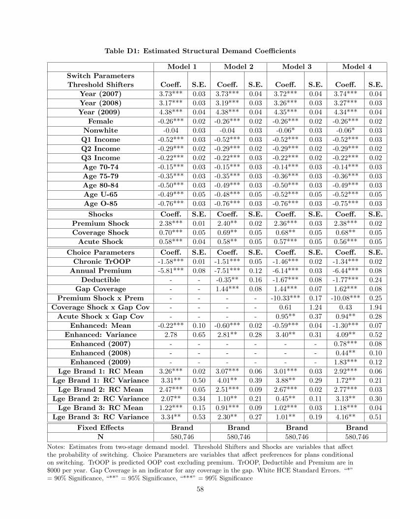
Table D1: Estimated Structural Demand Coefficients
Model 1 Model 2 Model 3 Model 4
Switch ParametersThreshold Shifters Coeff. S.E. Coeff. S.E. Coeff. S.E. Coeff. S.E.
Year (2007) 3.73*** 0.03 3.73*** 0.04 3.72*** 0.04 3.74*** 0.04
Year (2008) 3.17*** 0.03 3.19*** 0.03 3.26*** 0.03 3.27*** 0.03
Year (2009) 4.38*** 0.04 4.38*** 0.04 4.35*** 0.04 4.34*** 0.04
Female -0.26*** 0.02 -0.26*** 0.02 -0.26*** 0.02 -0.26*** 0.02
Nonwhite -0.04 0.03 -0.04 0.03 -0.06* 0.03 -0.06* 0.03
Q1 Income -0.52*** 0.03 -0.52*** 0.03 -0.52*** 0.03 -0.52*** 0.03
Q2 Income -0.29*** 0.02 -0.29*** 0.02 -0.29*** 0.02 -0.29*** 0.02
Q3 Income -0.22*** 0.02 -0.22*** 0.03 -0.22*** 0.02 -0.22*** 0.02
Age 70-74 -0.15*** 0.03 -0.15*** 0.03 -0.14*** 0.03 -0.14*** 0.03
Age 75-79 -0.35*** 0.03 -0.35*** 0.03 -0.36*** 0.03 -0.36*** 0.03
Age 80-84 -0.50*** 0.03 -0.49*** 0.03 -0.50*** 0.03 -0.49*** 0.03
Age U-65 -0.49*** 0.05 -0.48*** 0.05 -0.52*** 0.05 -0.52*** 0.05
Age O-85 -0.76*** 0.03 -0.76*** 0.03 -0.76*** 0.03 -0.75*** 0.03
Shocks Coeff. S.E. Coeff. S.E. Coeff. S.E. Coeff. S.E.
Premium Shock 2.38*** 0.01 2.40** 0.02 2.36*** 0.03 2.38*** 0.02
Coverage Shock 0.70*** 0.05 0.69** 0.05 0.68** 0.05 0.68** 0.05
Acute Shock 0.58*** 0.04 0.58** 0.05 0.57*** 0.05 0.56*** 0.05
Choice Parameters Coeff. S.E. Coeff. S.E. Coeff. S.E. Coeff. S.E.
Chronic TrOOP -1.58*** 0.01 -1.51*** 0.05 -1.46*** 0.02 -1.34*** 0.02
Annual Premium -5.81*** 0.08 -7.51*** 0.12 -6.14*** 0.03 -6.44*** 0.08
Deductible - - -0.35** 0.16 -1.67*** 0.08 -1.77*** 0.24
Gap Coverage - - 1.44*** 0.08 1.44*** 0.07 1.62*** 0.08
Premium Shock x Prem - - - - -10.33*** 0.17 -10.08*** 0.25
Coverage Shock x Gap Cov - - - - 0.61 1.24 0.43 1.94
Acute Shock x Gap Cov - - - - 0.95** 0.37 0.94** 0.28
Enhanced: Mean -0.22*** 0.10 -0.60*** 0.02 -0.59*** 0.04 -1.30*** 0.07
Enhanced: Variance 2.78 0.65 2.81** 0.28 3.40** 0.31 4.09** 0.52
Enhanced (2007) - - - - - - 0.78*** 0.08
Enhanced (2008) - - - - - - 0.44** 0.10
Enhanced (2009) - - - - - - 1.83*** 0.12
Lge Brand 1: RC Mean 3.26*** 0.02 3.07*** 0.06 3.01*** 0.03 2.92*** 0.06
Lge Brand 1: RC Variance 3.31** 0.50 4.01** 0.39 3.88** 0.29 1.72** 0.21
Lge Brand 2: RC Mean 2.47*** 0.05 2.51*** 0.09 2.67*** 0.02 2.77*** 0.03
Lge Brand 2: RC Variance 2.07** 0.34 1.10** 0.21 0.45** 0.11 3.13** 0.30
Lge Brand 3: RC Mean 1.22*** 0.15 0.91*** 0.09 1.02*** 0.03 1.18*** 0.04
Lge Brand 3: RC Variance 3.34** 0.53 2.30** 0.27 1.01** 0.19 4.16** 0.51
Fixed Effects Brand Brand Brand Brand
N 580,746 580,746 580,746 580,746
Notes: Estimates from two-stage demand model. Threshold Shifters and Shocks are variables that affectthe probability of switching. Choice Parameters are variables that affect preferences for plans conditionalon switching. TrOOP is predicted OOP cost excluding premium. TrOOP, Deductible and Premium are in$000 per year. Gap Coverage is an indicator for any coverage in the gap. White HCE Standard Errors. “*”= 90% Significance, “**” = 95% Significance, “***” = 99% Significance
58

Appendix Table D2: Descriptive Statistics for Demand Model Variables
Switch Parameters
Threshold Shifters Variable Mean Standard Deviation
Constant 1.000 0.000
Female 0.619 0.486
Nonwhite 0.091 0.287
Q1 Income 0.225 0.417
Q2 Income 0.269 0.443
Q3 Income 0.255 0.436
Age 70-74 0.198 0.398
Age 75-79 0.179 0.383
Age 80-84 0.159 0.365
Age U-65 0.061 0.240
Age O-85 0.163 0.370
Shocks Variable Mean Standard Deviation
Premium Shock -0.266 0.442
Coverage Shock -0.024 0.154
Acute Shock -0.037 0.189
Choice Parameters Variable Mean Standard Deviation
Chronic TrOOP($000) 0.784 0.935
Acute TrOOP ($000) 0.105 0.128
Premium ($000) 0.471 0.241
Deductible ($000) 0.095 0.126
Gap Coverage 0.235 0.424
Premium Shock x Premium 0.127 0.247
Coverage Shock x Gap Coverage 0.006 0.079
Acute Shock x Gap Coverage 0.010 0.098
Enhanced 0.472 0.499
Enhanced (2006) 0.072 0.258
Enhanced (2007) 0.122 0.328
Enhanced (2008) 0.135 0.342
Enhanced (2009) 0.143 0.350
Notes: Summary statistics for variables included in two-stage model of choice and switching. Premium,Coverage and Acute Shocks defined in Section 5.2. Gap Coverage is an indicator for any coverage in thegap.
59

Appendix Table E1: The Five Largest New Jersey PDP Plans, 2006
Insurer Name Plan Name Market Share
United Healthcare AARP MedicareRx Plan 27.63%
Horizon Blue Cross Blue Shield of NJ Horizon Medicare Rx Plan 2 25.40%
Humana Insurance Company Humana PDP Standard S5884-062 10.13%
First Health Premier First Health Premier 4.56%
Humana Insurance Company Humana PDP Enhanced S5884-003 4.15%
Notes: Publicly available data on names and market shares of the five largest New Jersey PDP plans in2006. Source: CMS.
Appendix Table E2: Premium Dispersion in New Jersey DSB Plans
Mean, Equal Std. Dev., Equal Mean, Weighted Std. Dev., Weighted Minimum Maximum
2006 $26.33 $11.33 $9.27 $10.52 $4.43 $35.49
2007 $31.28 $12.44 $10.37 $1.86 $10.20 $47.40
2008 $32.51 $17.61 $31.28 $6.19 $19.20 $69.00
2009 $42.88 $18.08 $29.84 $10.46 $26.60 $72.70
2010 $37.66 $4.88 $32.84 $2.21 $32.00 $42.90
2011 $39.73 $5.73 $37.26 $3.17 $34.20 $47.60
2012 $38.37 $4.20 $37.32 $4.48 $34.80 $43.00
Notes: Summary of premium dispersion in NJ Defined Standard Benefit plans. Premiums are in $ perenrollee per month. “Weighted” means weighted by enrollment.
Appendix Table E3: Annual Premium Increases ($), Accounting for “Sister” PlanEntry
Model 1 Model 2 Model 3
Coeff. SE Coeff. SE Coeff. SE
Lagged Premium -0.165*** 0.008 -0.154*** 0.009 -0.162*** 0.008
Lagged # Tier 1 Drugs 0.031*** 0.005 0.028** 0.005 0.030** 0.005
Lagged Deductible -0.007*** 0.001 -0.008*** 0.001 -0.008*** 0.001
Lagged Enhanced 1.623*** 0.334 1.322*** 0.338 1.529*** 0.335
Lagged Gap Coverage 5.505*** 0.396 5.194*** 0.399 5.418*** 0.397
Lagged Market Share 6.716*** 1.228 6.749*** 1.225 6.725*** 1.227
Enrollment Growth Rate -4.001** 1.154 -3.558*** 1.154 -3.735** 1.155
Enter “Sister” Plan - - -2.038*** 0.342 - -
Enter low-prem “Sister” Plan - - - - -1.876*** 0.516
Brand FE? Yes Yes Yes
Region FE? Yes Yes Yes
N 7,796 7,796 7,796
R2 0.274 0.276 0.274
Notes: Regression of premium increase (in $) on previous-year plan characteristics (national data). Enroll-ment growth rate is rate of growth for region’s Part D program. Lagged market share is for this plan. Enter“Sister” plan is an indicator for same carrier adding a new plan in the relevant year; Enter low-prem “Sister”plan is an indicator for adding a new plan whose premium is the lowest in the market for that carrier.
60

E Details on Counterfactual Simulation
In order to simulate plan pricing in the counterfactual, we first must construct an estimate
of plan costs that accounts for manufacturer rebates. In each year for each drug observed in the
prescription drug event file, we categorize the drug as either branded or generic. For drugs that
cannot be categorized, we label them as generic if their average cost is below the median among
uncategorized drugs. Then for each branded drug and each year we generate the average cost
per day’s supply of the drug and apply it to each observed prescription, scaled by the observed
supply length. We assume the cost net of rebates is 80% of this amount55. For generic drugs, we
assume the cost is $4 per month’s supply and scale by the observed supply length56. For drug
events in the catastrophic phase, we assume the plan pays 15% and the beneficiary pays 5%, while
for all other events we treat the beneficiary’s TrOOP payment as known. We sum these drug
costs over beneficiaries to generate an estimated annual cost figure and annual TrOOP for each
beneficiary. Then within each plan and year we winsorize by replacing estimated annual costs and
annual TrOOP for the bottom 2.5% of beneficiaries with the 2.5% quantile, and analogously for
the top 2.5%. These winsorized annual figures are then averaged within plan and year to generate
estimates of benefit cost and TrOOP per covered life. Applying an administrative cost assumption
of 16% of drug costs57, we generate an estimate of total costs per covered life net of TrOOP, which
is treated as Cj,t in Equation (4).
The second step in our simulation is to refine our estimates of each individual’s unobserved type
by using the information from their observed choices. Each individual i has random preferences
θRC,i ∼ MVN(θRC ,ΣIRΣ′). Denoting the distribution of random preferences as a function of our
estimated parameters as F (θRC,i|θC , Σ) with associated density f and the observed sequence of
choices for individual i as CObsi , we can write the conditional distribution of the individual’s type
as:
P (θRC,i|CObsi ) =P (CObsi |θRC,i, Θ)f(θRC,i|θC , Σ)∫
θRCP (CObsi |θRC , Θ) ∂F (θRC |θC , Σ)
Given Θ and θRC,i we can compute the likelihood of a given sequence of choices CObsi directly using
the formulas from Appendix D.3. We use this approach to construct the conditional density using
simulation, approximating the integral in the denominator with S′ = 50 simulation draws and
drawing S = 10 values {θR,sC,i }Ss=1 from the conditional distribution for each individual.
Finally we use these inputs to solve for each plan’s optimal bid under each counterfactual. Con-
55A study by the Department of Health and Human Services Inspector General (Levinson (2011)) found that, in2009, rebates reduced Part D drug expenditures by 19% on average for the 100 highest-volume brand name drugs.We assume a slightly lower percentage to account for potentially lower rebates for lower-volume drugs.
56Our assumption for generic drug costs is based on Walmart’s well known “$4 for any generic prescription”program.
57Sullivan (2013) notes that the National Health Expenditure Accounts (NHEA) includes the administrative costsof Medicare Advantage plans and Part D plans in its report of total Medicare administrative costs. We use this fact,and data from the NHEA for 2006-2010, to back out administrative expenses of 14-16% of total costs - or 16-19% ofnon-administrative costs - for Parts C and D combined.
61

ditional on their unobserved type θRC,i (and the premium coefficient for the relevant counterfactual),
the choice probability of each individual for each plan-year in our static simulations takes the simple
logit form:
Λi,j,t =eXC,i,j,tθ
NRC +XR
C,i,j,tθRC,i
ΣKtk=1 e
XC,i,k,tθNRC +XR
C,i,k,tθRC,i
while the unconditional probability is the integral over the filtered distribution from step 2:
Λi,j,t =
∫θRC,i
Λi,j,t P (θRC,i|CObsi ) ∂θRC,i
Plan j’s enrollment in year t under the counterfactual is therefore:
Nj,t = ΣNti=1 Λi,j,t
where Nt is the number of beneficiaries active in year t.
Denote the bid, base premium, enhanced premium and costs for plan j in year t by Bj,t, Pj,t,
Ej,t, and Cj,t, respectively. Plan profits are a function of the bid, enhanced premium, costs, and
enrollment, and plans choose their bid to maximize profit:
Bj,t = ARGMAXB
πj,t = (B + Ej,t − Cj,t)Nj,t
subject to the restriction that their premiums are determined by the Medicare Part D bidding
mechanism, and are constrained to lie above zero:58
Pj,t = Bj,t −NAMBAt +BBPt + Ej,t
BBPt = BPPt ×NAMBAt
NAMBAt =1
JtΣJtk=1 Bk,t
Pj,t ≥ 0
Under the assumption that the Base Premium Percentage (BPPt), enhanced premium and costs
are exogenous, we can write the plan’s premium in terms of its own and all other plans’ bids,
yielding an expression for the derivatives of plan premiums with respect to own- and other-plan
bids:
∂Pj,t∂Bj,t
=Jt − (1−BPPt)
Jt∂Pk,t∂Bj,t
=−(1−BPPt)
Jt
58This is a simplification of the true system in which the base premium, not the total including the enhancedpremium, is constrained to be weakly greater than zero.
62

Conditional on θRC,i, the derivative of the choice probability with respect to plan premiums is of the
usual logit form:
∂Λi,j,t∂Pj,t
= β2,1Λi,j,t(1− Λi,j,t)
∂Λi,j,t∂Pk,t
= −β2,1Λi,j,tΛi,k,t
where β2,1 is the utility parameter for plan premiums.
Combining the expressions above, we can write the plan’s optimal bidding problem as:
MAXB
(B + Ej,t − Cj,t)× (ΣNti=1 Λi,j,t)
s.t. B ≥ −Ej,t +1−BPPt
JtΣJtk=1 Bk,t
where Ei,t, BPPt and Jt are given. We can derive a first-order condition for the plan’s bidding
decision as:
∂πj,t∂Bj,t
= (Bj,t + Ej,t − Cj,t)∂Nj,t
∂Bj,t+Nj,t = 0
where
∂Nj,t
∂Bj,t= ΣNt
i=1 β2,1[
∫θRC,i
Λi,j,t(1− Λi,j,t) P (θRC,i|CObsi ) ∂θRC,i]Jt − (1−BPPt)
Jt
+ Σk 6=j β2,1[
∫θRC,i
Λi,j,tΛi,k,t P (θRC,i|CObsi ) ∂θRC,i](1−BPPt)
Jt
We solve for each plan’s choice of bids, and hence premiums, by solving the system of first-order con-
ditions expressed above using Gauss-Jacobi and SQP. In each step, we solve each plan’s constrained
optimization problem using the current-iterate bids and the expressions for the bidding mechanism
above, and then generate choice probabilities and update the bid accordingly. Choice probabilities
are generated using Model 4 from Table D1, where we assume that the shock interaction effects are
all zero, and we use the observed Base Premium Percentage in each year.
Some of the inputs to this analysis need to be imputed from the data. We observe PDP plan
total and basic premiums for NJ and infer enhanced premiums as the difference between the two.
The NAMBA, Base Beneficiary Premium and Base Premium Percentage are published annually
by CMS, and in the years over which we simulate, they are, respectively, ($92.30, $32.20, 34.88%) in
2006, ($80.43, $27.35, 34.00%) in 2007, ($80.52, $27.93, 34.68%) in 2008, and ($84.33, $30.36, 36.00%)
in 2009. For the purposes of determining monthly per-member subsidies, plan bids are actually
scaled by a risk metric (RxHCC) that varies depending on the average demographic and chronic
conditions of the insurer’s risk pool. We ignore this metric, assuming that the government reinsur-
ance program removes any incentives that may result from the scaling, and assume that each plan is
63

paid their bid (Bj,t) plus their enhanced premium (Ej,t). We assume the enhanced premium is held
fixed at observed levels. The NAMBA is a national average over all MA-PD and PDP plans. We
use our NJ data, and the observed total number of MA and PDP plans included in the NAMBA,
to back out the national sum of MA bids under the assumption that MA and non-NJ PDP plans
have the same average bids. We hold MA plan bids fixed in our calculations. We assume that
non-NJ PDP plan bids change by the same percentage, on average, as the predicted change for NJ
PDP plans.
64


