
The influence of bank capital on the lending behavior
Credit channels in the U.S.
K. (Karim) Harakeh1
UNIVERSITY OF GRONINGEN
Faculty of Economics and Business
MSc Business Administration, Specialization Finance
Supervisor: prof. dr. K.F. (Kasper) Roszbach
June 2013, Groningen
Abstract
I collect quarterly data from the Call Reports, which all insured banks are required to submit
to the Federal Reserve each quarter. Using these reports I analyze the effects of monetary
policy changes and macroeconomic factors on the lending behavior of banks. I find evidence
of a bank lending channel and a bank capital channel of monetary policy in the U.S. from Q4
2002 to Q4 2012. My research also provides empirical evidence that bank capital plays an
important role in the context of the credit channels. Furthermore, banks seem to be exposed
to GDP growth where it appears that well-capitalized banks are better able to insulate the
effects of GDP on their lending compared to low-capitalized banks.
JEL classification: E44; E52; G21
Keywords: monetary policy; monetary transmission mechanisms; bank lending; bank capital
1 Student number: s2181681 Email: [email protected]

K. Harakeh | University of Groningen 1
Table of Contents
1. Introduction ........................................................................................................................................ 2
2. Literature overview ............................................................................................................................. 4
2.1 General overview ........................................................................................................................... 4
2.2 The role of bank capital .................................................................................................................. 8
2.3 Monetary policy ............................................................................................................................. 9
3. Hypotheses........................................................................................................................................ 10
4. Methodology ..................................................................................................................................... 11
4.1 Endogeneity problem................................................................................................................... 11
4.2 Methodological approach ............................................................................................................ 11
5. Data description ................................................................................................................................ 14
6. Results ............................................................................................................................................... 18
7. Robustness checks ............................................................................................................................. 21
8. Conclusion ......................................................................................................................................... 23
References ........................................................................................................................................ 25
Appendix A ........................................................................................................................................ 28
Appendix B ........................................................................................................................................ 30
Appendix C ........................................................................................................................................ 31
Appendix D ........................................................................................................................................ 31
Appendix E ........................................................................................................................................ 32

K. Harakeh | University of Groningen 2
I. Introduction
Banks as “financial intermediaries” have a pivotal role in the economy as they provide lending to firms
and households. In fact, their role as providers of credit is particularly crucial in economic downturns and
financial distress. However, in reality during recessions banks seem to do the opposite of what is desired
namely issuing fewer loans. This phenomenon in bank lending can be caused by either the reluctance of
banks to lend money as they become more risk-averse, or because of the negative impact that a recession
has on the creditworthiness of borrowers which makes potential borrowers ineligible for bank loans.
There are several factors that could influence the lending behavior of banks. One factor, as is already
mentioned in the first paragraph, has to do with macroeconomic factors such as GDP growth. Monetary
policy changes are another factor, which may also play a very important role, since monetary policy aims
at influencing the availability and cost of money and credit in order to stimulate lending in times of
recession and discourage lending in prosperous economical periods (i.e. to avoid overheating of the
economy). This means that the Federal Reserve (Fed) would intervene by conducting monetary policies
with the intention to keep the balance of credit intact and foster stable economic growth. Furthermore, the
Fed has several monetary tools at its disposal with the purpose to set a target for the key interest rate, i.e.
the federal funds rate. At the moment of writing, the Fed is maintaining the federal funds rate at 0% since
the fourth quarter of 2009 as a reaction to the financial crisis that hit the U.S. economy. The magnitude of
the crisis was unprecedented causing Lehman Brothers, a giant in the financial sector, to collapse which
was the largest bankruptcy filing in the U.S. history. The federal funds rate has never been so low for such
a long time period, which is a consequence of the prolonged financial crisis. This can be interpreted as an
expansionary policy of the Fed with the aim to increase bank lending since this is one of the driving
factors behind economic growth.
Credit effects of monetary transmission mechanisms, which mediate between monetary policy processes
and their results on the economy, have been taken into account in the recent past. For example, studies by
Bernanke and Blinder (1988) and Kashyap, Stein, and Wilcox (1993) contributed to the literature by
introducing the bank lending channel as a monetary transmission mechanism. At the time, they only
focused on the effect of a change in reserve requirements on the deposits of a bank in order to explain
changes in bank lending. Interestingly, bank capital was being considered as an unimportant interaction
factor to determine the change in the bank‟s lending behavior (Friedman, 1991). This, however, changed
at the beginning of this century through works of Jayaratne and Morgan (2000) and Kishan and Opiela
(2000). They claimed that bank capital is an important balance-sheet item that enhances the capacity to

K. Harakeh | University of Groningen 3
raise non-deposit sources of funds and therefore banks‟ ability to limit the effect of a drop in deposits on
lending. Since then, much research has been done on the effect of monetary policy on the lending
behavior of banks taking bank capital into account.
In this paper, I will mainly study the effect of monetary transmission mechanisms on bank lending.
Studies of the “traditional” monetary transmission mechanism initially focused on how a change in the
reserves alters interest rates and deposits which would lead to a persistent change in the overall spending.
My paper will focus similar to the work of Gambacorta and Mistrulli (2004) on two transmission
channels which are the bank lending channel and the bank capital channel. In the analysis of the bank
lending channel, I will use the excess risk-based capital of banks to investigate whether changes in the
monetary policy have affected bank lending due to the different capitalization ratios of banks. The
thought underlying this channel is that banks with higher capital ratios will find it easier to raise new
funds, in a situation where deposits decrease or other forms of reduction occur on the liability side of the
bank‟s balance sheet, compared to low-capitalized banks. Next, I will discuss the bank capital channel.
The notion underlying this theory is that monetary policy changes could affect the bank‟s capital through
the maturity transformation (exposure of interest rate risk) of the bank. The role of capital in the bank
capital channel is as follows: due to a monetary tightening, banks will see their profits as well as capital
accumulation decrease, and if issuing new shares is too costly, banks would adjust their lending in order
to meet the capital regulation requirements. Thus, the channels to be analyzed assume that capital plays an
important role in the lending behavior of banks. The research question of this thesis, which is an
extension of the work of Gambacorta and Mistrulli (2004) by including a larger and different dataset of
banks, is formulated as follows: “How has bank capital influenced the bank lending in the U.S. as a
consequence of monetary policy and macroeconomic changes between Q4 2002 and Q4 2012?” More
specifically, the main purpose of this study is to empirically investigate this question. My study differs
principally from the work of Gambacorta and Mistrulli (2004) in two ways: first, they include in their
analysis in addition to Italian banks a sample of Italian credit cooperatives and second, they use the
Generalized Method of Moments (GMM) estimator in their analysis whereas I use the Least Square
Dummy Variables (LSDV) model.
The outline of the paper is as follows: Section II provides the literature overview of previous research
related to this subject. Section III lists the hypotheses to be tested. Section IV describes the methodology
and the regression to be estimated and addresses the endogeneity problem. Section V explains how the
data have been collected. Section VI presents the findings and results of the study and Section VII
includes the robustness checks. Finally, Section VIII summarizes the findings in the conclusion part.

K. Harakeh | University of Groningen 4
II. Literature overview
2.1 General overview
In the existing literature, a lot of research has been reported which examines the monetary transmission
channels that explain how monetary policy decisions affect the real economy. In theory, there are at least
two different ways in which the level of bank equity can amplify the impact of monetary changes on bank
lending. Firstly, bank lending can be affected through the conventional bank lending channel. Secondly, it
can be affected through a more direct mechanism denoted as the bank capital channel. Interestingly, both
theories rely on imperfect credit markets. This is in contrast to the proposition of the Modigliani-Miller
theorem for banks which we will discuss later in this section.
Previous empirical literature studying the effect of bank capital on lending is predominantly focused on
the U.S. banking system (Furfine, 2000; Hancock et al., 1995; Kishan and Opiela, 2000; Van den Heuvel,
2001b). What these articles have in common is that they find evidence that bank capital is of great
importance in influencing the lending behavior of commercial banks. In addition, an early study of
Friedman and Schwartz (1963) has found evidence that monetary policy actions are followed by
movements in real economic output that may last for two years or more, implying that the lending
behavior of banks also gets affected by these actions. Similarly, Thakor (1996), who used an asymmetric-
information model of bank lending and simultaneously maintained the assumption of costly external
funds, has shown that monetary policy impacts bank lending. Furthermore, Bernanke and Blinder (1992)
proved in a very prominent paper that interest-rate shocks affect the size and composition of the bank‟s
portfolio (securities and loans) with a lag in time starting half a year later and lasting up to two years.
According to the Modigliani-Miller theorem, shocks to the liability side of a bank‟s balance sheet should
not make a bank reluctant to provide loans at any interest rate. This is consistent with the findings of
Romer and Romer (1990) in which they claim that banks can always find alternative sources of finance
other than deposits, meaning non-deposit (uninsured) sources of funds.2 Thus, even though the Fed is
2 Deposit accounts in the U.S. are insured by the Federal Deposit Insurance Corporation (FDIC), which is an
independent agency of the federal government created in 1933 in response to the thousands of bank failures in
the early 1920s and 30s. The FDIC insures all kinds of deposit accounts at an insured bank. The basic limit on
federal deposit insurance is since 2008 held at $250,000 (in 1980 it was $100,000). However, in order to receive
benefits, FDIC–insured banks must adhere to certain liquidity and reserve requirements. For example, when a bank
becomes undercapitalized and enters the danger zone of becoming insolvent (i.e. a risk-based capital ratio of <
8%), the bank will receive a warning from FDIC. In addition, when the capital ratio decreases to below the 6% level,
the primary regulator can interfere with the internal affairs of the bank by reappointing the management and
forcing the bank to change its policy.

K. Harakeh | University of Groningen 5
following a contractionary monetary policy, banks will still be able to raise funds, for example by issuing
new Certificates of Deposit (CD) to compensate for the shortfall in deposits. The bottom line of the work
of Romer and Romer (1990) is that bank‟s loan supply is completely unaffected by monetary policy.
The bank lending channel hypothesis suggests that due to imperfect markets, which prevent banks from
raising uninsured funds when exposed to contractionary monetary policy shocks, constrained banks will
find themselves in a position forcing them to adjust their lending. This is consistent with the findings of
Kashyap and Stein (1995) in which they claim that monetary policy will work in part through a lending
channel: when the Fed drains deposits from the system, financial intermediaries cannot make up the
funding shortfall without friction by raising non-deposit external finance, and this will eventually alter the
lending behavior of the banks. However, the bank lending channel indicates that well-capitalized banks
are in a better position to shield their lending from monetary policy shocks as they have easier access to
raising uninsured funds.
Moreover, due to the imperfect markets for bank debt and non-reservable liabilities, especially in
situations of financial distress or a negative outlook of the economy, a “lemon‟s premium” has to be paid
to investors. In this case, bank capital will be considered as an important item because lower capital levels
impact the creditworthiness of the bank and this in turn will lead to higher prices for uninsured liabilities
(Flannery and Sorescu, 1996). Therefore, the cost of wholesale funding (i.e. bonds or CDs) would be
higher for undercapitalized banks if they are perceived as being more risky by the financial market.
Another important factor that might weaken the bank lending channel is the existence of risk-based
capital requirements. Since a bank-capital‟s ability to absorb shocks is a measure of bank‟s health, and
therefore, is an indicator of a bank‟s ability to raise alternative external funding during periods of
monetary tightening. When a contractionary monetary policy takes place the lending of a capital-
unconstrained bank may either remain unaffected or even rise. In fact, Kishan and Opiela (2000) found
that the lending behavior of small undercapitalized U.S. banks (total assets <300M USD) is the most
responsive to monetary policy.
The bank capital channel can only exist due to imperfect capital markets similar to the situation with the
bank lending channel. According to the bank capital channel thesis, monetary policy affects bank lending
partly through its impact on bank capital (Van den Heuvel, 2002). In addition, Van den Heuvel (2001a)
showed in an earlier study that when capital is sufficiently low, because of high charge-offs (loan losses)
or some other adverse shocks, the bank will reduce lending due to the capital requirement of keeping a
certain percentage of the capital intact and also due to the high cost of issuing new shares. Although the
capital requirement is not stringent, the model of Van den Heuvel (2001a) shows that a low-capitalized

K. Harakeh | University of Groningen 6
bank may optimally pass profitable lending opportunities at a certain moment in order to reduce the risk
of future capital inadequacy. However, if banks were always able to raise new equity, no bank would ever
allow profitable lending opportunities to pass by and the capital requirements would be irrelevant except
insofar as equity has a higher required rate of return. Myers and Majluf (1984) provide theoretical
evidence to support the assumption that issuing new equity can be quite costly under certain
circumstances.
Banks confronted with binding capital constraints as a result of high charge-offs and low or no earnings
have only two options to increase their capital/asset ratios. The first method is by raising new capital (e.g.
issuing new common stock), and the second method is by shrinking mainly their assets (Peek and
Rosengren 1995). Furthermore, Hancock and Wilcox (1992) claim that losses of bank capital can cause
banks to shrink their assets and liabilities to restore target capital/asset ratios in response to regulatory
pressures, financial market pressures, or the tastes and preferences of bank management. In agreement
with Hancock and Wilcox (1992), Peek and Rosengren (1995) found evidence that there is a strong
positive relation between shocks to a bank's capital and the growth rate of its deposits. Accordingly, the
bank capital channel will be tested in this study by looking at the effect of the change in the bank‟s profit
on its capital.
Size of the commercial banks can also be a factor in the difference of the responsiveness to monetary
policy. Larger banks may have the advantage to raise capital less expensively than smaller banks due to
the economies of scale in equity issuance and also because the greater information flows of larger banks
may reduce investors‟ fears about adverse selection problem (Hancock et al., 1995). Furthermore, Peek
and Rosengren (1995) have seen that small banks have a larger proportion of loans to small companies
whose demands tend to be more pro-cyclical. In addition, smaller banks may rely relatively more on
reconstructing their portfolio compared to larger banks for rebuilding their capital ratios due to the higher
cost in raising capital. This means that smaller banks tend to decrease their assets by reducing loans,
giving rise to a phenomenon called “credit rationing”. This phenomenon can amplify the lending channel,
because banks may have the preference to issue large volume loans to a smaller number of high quality
borrowers, while the investment projects for the majority of bank-dependent borrowers with weaker
creditworthiness may not be funded (Stiglitz and Weiss, 1981). In agreement with this, Morgan (1998)
finds that large banks are often involved in loan commitments with big borrowers and are better able to
attract alternative (uninsured) funds in order to preserve the long-term lending relationships during
contractionary periods. This means that if credit rationing is not an important driver in the lending
behavior of banks, and if commitments and relationship lending protect borrowers from being excluded
from borrowing, then commitments deteriorate the effectiveness of the lending channel.

K. Harakeh | University of Groningen 7
Technically speaking, banks consider loans and securities as interchangeable assets. Therefore, when the
demand for loans strengthens, it is proposed that banks sell their securities in order to issue more loans.
This is in contrast with a weaker demand for loans, because in such scenario banks will tend to hold more
securities. Banks can use investments in securities to manage the interest-rate risk inherent in their core
business (Beatty and Bettinghaus, 1997). Furthermore, according to Kashyap and Stein (1995) the main
difference between loans and securities is that securities can be liquidated without costs. Due to this better
“liquidity” in equilibrium, banks would prefer to hold securities even when these offer an inferior return
compared to loans.
Another aspect, which plays an important role in bank performance, is bank governance. Looking at a
more recent study, Beltratti and Stulz (2012) found strong evidence that banks, which relied more on
deposits for their financing, and large banks, which had less leverage in 2006, performed better during the
crisis. In addition, some literature emphasizes that failings in bank governance played a major role in the
performance of banks (Diamond and Rajan, 2009, and Bebchuk, Cohen and Spamann, 2010). The idea is
that banks with poor governance were engaged in taking excessive risk which increased their market
exposure and resulted in larger losses during the crisis. Furthermore, Cornett et al. (2011) found that U.S.
banks with more exposure to liquidity risk experienced less loan growth during the crisis. Beltratti and
Stulz (2012) also found that banks with large stock returns in 2006 were the banks the stocks of which
suffered the largest losses during the crisis. This article also provides evidence that banks from countries
with stricter regulations in 2006 fared better during the crisis. This is understandable because banks with
more restrictions on their banking activities were able to achieve higher returns because they did not have
the opportunity to diversify into activities that unexpectedly performed poorly during the crisis.
Besides monetary policy shocks, bank lending is also exposed to macroeconomic influences. A reason for
this could be the high pro-cyclicality of credit. In fact, during recessions the amount of newly issued loans
reduces dramatically. This could be explained either by the supply side (bank lending channel) or by the
weakening of the demand for loans (a demand shift), or by both. Apart from that, the lending behavior of
banks could react differently with respect to the business cycle.
Studies by Boot (2000) and Thakor (2004) show that banks intensely involved in relationship lending
have the tendency to smooth lending “through the cycle”. Furthermore, well-capitalized banks could be in
a better position to deal with temporary financial difficulties that borrowers might face. In addition, bank
capital is an important factor in composing the loan portfolio. For instance, if banks issued loans that are
exposed to higher returns and risks this would imply that their borrowers are, on average, more exposed
to financial distress when the economy weakens. In addition, Kwan and Eisenbeis (1997) found evidence
K. Harakeh | University of Groningen 8
that capital is negatively correlated with credit risk. In other words, the loan supply of well-capitalized
banks is less dependent on the state of the economy compared to low-capitalized banks. This is consistent
with the findings of Flannery (1989) and Gennotte and Pyle (1991), who assert that better capitalized
banks are more risk-averse as they select their clients (w.r.t. loans) more carefully with the emphasis on
minimizing the probability of defaulting. As a result, during an economic recession, well-capitalized
banks would have relatively lower charge-offs and their capital level would change less due to the lower
unexpected losses in comparison with other banks.
2.2 The role of bank capital
Bank capital is important as it serves as the cushion to absorb any unexpected losses incurred by the bank.
It is basically the difference between the value of bank‟s assets and liabilities and it is also known as the
net worth of the bank. However, it also serves as the source for paying dividends to the shareholders in
times of high return. Thus, since the position of banks in any economy is pivotal, as suppliers of credit
and financial liquidity, so is bank capital. Therefore, banks are greatly regulated by the Fed, and their
capital is constantly subject to international regulatory rules directed by the Bank for International
Settlements (BIS), situated in Basel, Switzerland.
Total capital is comprised of retained earnings, reserves, equity capital, preference share capital, hybrid
capital instruments and subordinated debt. Total capital can be subdivided by Tier 1 and Tier 2 capital.
The former includes the first three items mentioned and the latter the last three items. Difference between
Tier 1 and Tier 2 capital ratios is that the former is considered to be the core (highest quality) capital as a
percentage of the bank‟s total assets adjusted for risk (risk-weighted assets) using global banking
guidelines. Tier 2 is considered to be the lower quality capital as it cannot serve to absorb losses and in
contrast to Tier 1 it is repayable and has a shorter term horizon than equity capital. As a study of Beltratti
and Stulz (2009) showed, large banks with (relatively) higher Tier 1 capital and more deposit financing at
the end of 2006 had significantly higher returns during the financial crisis 2007-2009.
In case of financial distress, banks can use their reserves, freeze dividends or in more extreme scenarios
write off equity capital. From a risk-management perspective, “capital” is an important driver when the
management of the bank wants to make important bank‟s decisions. This is especially true in periods of
financial distress in which capital targets imposed by bank‟s creditors or regulators become more
rigorous. Furthermore, bank capital has an important role because it affects the bank‟s external credit
ratings and provides the investors with a signal about their creditworthiness.

K. Harakeh | University of Groningen 9
2.3 Monetary policy
The Fed is the Central Bank of the U.S. which determines the U.S. monetary policy. The Fed is enabled
by law to undertake actions to influence the availability and cost of money and credit in order to maintain
sound economic policies to foster growth, sustainable employment and retain stable inflation levels. In
order to achieve its goals the Fed sets a target for a key interest rate, the federal funds rate, with the help
of the following three monetary policy tools: the reserve requirements (RR), the discount rate and the
open market operations. By employing these tools jointly or individually, the Fed is able to set and
control the supply of money and credit.
Monetary policy can be subdivided into two contradictory policies also known as the expansionary and
the contractionary policies. While the former policy aims to increase the supply of money in the economy,
the latter seeks the reverse. Both strategies work through the monetary transmission mechanism. This
means that when the Fed decides to change the RR, the discount rate and/or buy/sell bonds (or treasuries)
on the open market, it will impact the real economy, since it will affect the policies of the financial
intermediaries (i.e. the commercial banks) on their lending behavior. For example, in a recession (or
recessionary gap) it will be very likely that the Fed will foster economic growth by increasing the money
supply. Increasing the money supply leads to lower interest rates which in turn increase the amount of
investments in the economy due to more favorable borrowing conditions. This in turn will shift the
aggregate demand curve upwards in the macroeconomic setting. Important to mention here is that
expansionary monetary policy goes hand in hand with an increase in price levels, i.e. it has an inflationary
trend.
A contractionary monetary policy can take place when the Fed believes that the economy is overheating.
The tools they can apply to slow down the economy are increasing the RR, increasing the discount rate
and/or sell bonds (or treasuries) on the open market. This is clearly exactly the opposite of the case of an
expansionary policy. In addition, Cook and Hahn (1989a) confirm this effect through finding evidence
that when the Fed conducts contractionary open-market operations (i.e. selling bonds), interest rates for
fixed-income securities of all maturities typically rise, and thus make it less enticing to borrow money for
investments.
Thus, the Fed typically loosens policy when the economy slows down, and tightens it when the economy
grows. However, Lown and Morgan (2002) argue that it is difficult to identify the effects of the monetary
policy due to its endogenous response to economic conditions.

K. Harakeh | University of Groningen 10
III. Hypotheses
The above observations made in the literature motivate me to propose the following hypotheses, which I
will test in this thesis. The first hypothesis has to do with testing the bank lending channel.
H1: The impact of monetary policy actions differs amongst banks with a different degree of
capitalization.
The second hypothesis considers the bank capital channel. The underlying thought is that a reduction in
the bank‟s capital accumulation might have a negative impact on bank lending. This thesis hypothesizes
that a change in profitability alters the capital accumulation and hence the bank lending.
H2: Bank lending is influenced by a change in profitability giving rise to the bank capital
channel.
The last hypothesis is related to the difference in risk behavior of banks. The propagated idea is that well-
capitalized banks are more risk-averse as they can select their clients, thus minimizing their risks. This
hypothesis in which banks with higher capital levels are expected to be more risk-averse can also be
substantiated by considering capital as a cushion against certain economic scenario‟s (Dewatripont and
Tirole, 1994; Repullo, 2000; Van den Heuvel, 2001a). On the other hand, bank lending of low-capitalized
banks are more dependent on the state of the economy as their bank lending tend to be more exposed to
risks.
H3: There is difference in risk behavior amongst banks with a different degree of capitalization.
These hypotheses will be further discussed in the following section in the light of the methodological
approach.
K. Harakeh | University of Groningen 11
IV. Methodology
4.1 Endogeneity problem
Endogeneity is a common problem in research that cannot be neglected in estimating (financial) models.
In fact, it threatens the validity of models that make causal claims regarding the relationship between the
independent variable(s) and the dependent variable.
Having a strong correlation and significant relationship between the independent and dependent variables
does not necessarily mean that it reflects a true relationship. The problem is that the independent variables
may not be independent after all and that there exists a two-way relationship of dependence between the
variables. This indicates a situation of an omitted course which is not observable. In order to tackle this
endogeneity problem, all the regressors related to the bank specific characteristics will refer to those of
the (t – 1) quarter to avoid an endogeneity bias.
Taking the above into consideration, I performed a Hausman (endogeneity) test in the model described in
the following subsection in order to check whether the explanatory variables in the regression are actually
exogenous. This test allows me to determine which is applicable: the random effects or the fixed effects.
By conducting the Hausman test, I obtained a p-value of 1 indicating that both random and fixed effects
are applicable.
Endogeneity can have different causes, but it especially occurs by omitting variables and introducing
fixed effects into the model can greatly reduce the probability that a relationship is driven by an omitted
variable.
4.2 Methodological approach
This study employs the LSDV regression with cross-sectional fixed effects to perform empirical research
on the impact of monetary policy effects and macroeconomic changes on the lending behavior of banks.
The model can also be described as a dynamic panel-data model due to the use of lagged-dependent
variables as regressors. In literature, a popular model to estimate dynamic panel data is the GMM
estimator suggested by Arrelano and Bond (1991), which is designed for panel data consisting of a large
number of banks (N) and a small number of quarters (T). The latter model allows for endogeneity among
the independent variables by introducing instrumental variables. However, this model is very complicated
and can easily generate invalid outcomes.
Applying LSDV regression can lead to an endogeneity bias in which the lagged-dependent variables are
endogenous to the fixed effects in the error term giving rise to the “dynamic panel bias”. However, since
K. Harakeh | University of Groningen 12
the sample contains 41 time periods, which is relatively large, the impact on the bank‟s apparent fixed
effect would decrease together with the endogeneity problem. In addition, Roodman (2006) confirmed
that a sample with a large (T) will remove the dynamic panel bias, and a more straightforward fixed
effects estimator would be appropriate.3 Moreover, data were transformed into first-differences in order to
make the estimation more consistent and to function as a potential remedy for auto-correlated residuals.4
To test whether auto-correlation in my sample is under control, I estimated the LSDV model in two
different ways with and without robust standard errors and noticed that there were no big differences in
the computed standard errors. Furthermore, coefficient standard errors are adjusted by employing panel-
corrected standard errors in order to control for heteroskedasticity.
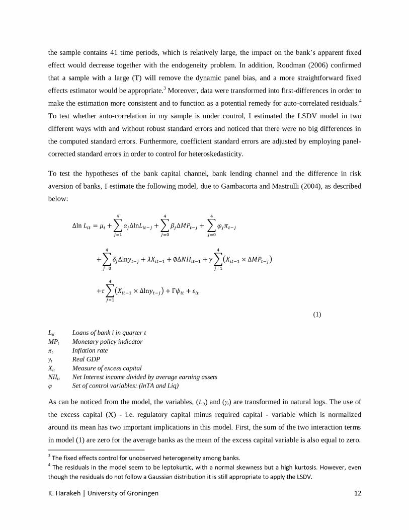
To test the hypotheses of the bank capital channel, bank lending channel and the difference in risk
aversion of banks, I estimate the following model, due to Gambacorta and Mastrulli (2004), as described
below:
∑
∑
∑
∑
∑( )
∑( )
(1)
Lit Loans of bank i in quarter t
MPt Monetary policy indicator
πt Inflation rate
γt Real GDP
Xit Measure of excess capital
NIIit Net Interest income divided by average earning assets
φ Set of control variables: (lnTA and Liq)
As can be noticed from the model, the variables, (Lit) and (γt) are transformed in natural logs. The use of
the excess capital (X) - i.e. regulatory capital minus required capital - variable which is normalized
around its mean has two important implications in this model. First, the sum of the two interaction terms
in model (1) are zero for the average banks as the mean of the excess capital variable is also equal to zero.
3 The fixed effects control for unobserved heterogeneity among banks. 4 The residuals in the model seem to be leptokurtic, with a normal skewness but a high kurtosis. However, even
though the residuals do not follow a Gaussian distribution it is still appropriate to apply the LSDV.
K. Harakeh | University of Groningen 13
Second, the meaning of the coefficients βj and δj can be easily interpreted as the average effect of
monetary policy and GDP, respectively. Furthermore, all the bank-specific variables (X, NII, lnTA and
Liq) in my estimation are stated in lags (t-1) to prevent endogeneity. In fact, lagged variables are by
nature exogenous, since an occurrence in the future cannot influence the past. Additionally, the macro-
economic factors in my model are assumed to be strictly exogenous.
This linear model estimates long-run coefficients, to test the effect of monetary policy (∑ )5
,
inflation (∑ ) and GDP changes (∑
).
6 Since these variables are assumed to be strictly
exogenous, as a two-way relationship is excluded, also t=0 on top of the four lags will be added in order
to calculate the long-run coefficients. Additionally, the equation includes the first-difference of Net
Interest Income (NII) of the previous quarter in order to investigate the presence of the bank capital
channel (see Appendix A). Following Gambacorta and Mistrulli (2004), I also considered the two
interaction terms being the product of excess capital with monetary policy and excess capital with GDP
changes, to examine the bank lending channel and the difference in risk behavior, respectively.
The presence of multicollinearity has been checked among the independent variables and no abnormal
correlations have been found.7 The stationarity of the dependent and independent variables has also been
taken into consideration by performing the unit root test suggested by Levin and Lin (1992). Fortunately,
all the variables are stationary and do not to follow a unit root process (p-value < 0.01) as this could lead
to spurious regressions.
5 The long-run elasticity of lending with respect to monetary policy, GDP shocks and inflation is calculated by
∑ ( ∑
)
6 Dummy variables are included to examine the degree to which seasonality is present and to remove any possible
serial correlation in which the residual structure is cyclical in shape. 7 The correlations between regressors are in the boundary of -0.3 ≤ ρ ≤ 0.3, except for the correlation between the
GDP variable and the MP indicator which has a ρ=0.6 and is just acceptable.

K. Harakeh | University of Groningen 14
V. Data description
Bank specific data used in the present estimation have been retrieved from the Reports of Condition and
Income, also known as the “Call Reports” 8, collected by the FDIC. All insured “commercial” banks and
savings associations in the U.S. are required to submit accurate financial data regarding their current
financial position and their operational results on a quarterly basis. This dataset of financial institutions is
of importance for this thesis as it focuses on activities based on deposits and loans. The data collected for
this study are quarterly and cover a time span from the fourth quarter of 2002 to the fourth quarter of
2012. This means that the dataset includes 41 time periods (T=41).
The sample consists of 2,875 FDIC insured banks (N=2,875). The composition of the sample has been
determined by the imposition of a few selection criteria in order to obtain appropriate data for the
estimation. First, banks were only included if a significant proportion of their portfolio consisted of loans
(i.e. banks should have had at least 35% of their portfolio consisting of loans during the whole period).
Second, Mergers and Acquisitions (M&A) were accounted for by removing all banks that experienced an
increase of 15% in total assets in a consecutive period. In addition, banks that showed an extraordinary
decrease or increase in the (12 month) loan growth rate are eliminated from the sample also to remove
any possible bias due to M&As.9 Naturally, a more professional way would be to filter out the data
regarding M&A activities by using M&A files. However, this method is beyond the scope of this study
because of lack of access to the data and therefore the assumption is adopted that if total assets increase
by 15% compared to the preceding period it would pertain to M&A activities. This assumption may bias
the results in case medium-sized banks indeed realize more than 15% growth without M&A, but I expect
the numbers of such banks that experience a 15% growth in total assets to be small. Third, the sample
only includes banks where all information (such as bank‟s loans, excess capital, liquidity, etc.) is
available in the Call Reports with respect to the input variables required to perform the regression
analyses as in equation (1). Fourth, only the banks that are completely covered in the Call Reports in the
period starting from Q4 2002 to Q4 2012 are included, thus for 41 periods. This eliminates banks from
the sample that went bankrupt or stopped their banking activities during the period in question. Due to the
latter selection criteria each bank now has the same number of time observations (also known as
“balanced panel data”) yielding a total of 117,875 observations. Finally, a small number of illogical
extreme outliers were removed that might affect the results of the analyses negatively.
8 The Call Reports have been downloaded from the official website of the FDIC 9 The boundaries were set at -30% and +38% as the intervals in the sample increased drastically after these levels.

K. Harakeh | University of Groningen 15
The dependent variable used in the estimations is the “total gross loans” of banks and will be denoted as
(Lit). Furthermore, an independent variable representing the excess capital will be included. However, this
variable will be adjusted in a way to test for the existence of asymmetric effects due to bank capital by the
following normalization adjustment as proposed by Gambacorta and Mistrulli (2004):
(∑
∑
) (2)
where (EC) and (RWA) stand for excess capital (Regulatory capital – capital requirements) and risk-
weighted assets, respectively.10
Furthermore, i and t are indices running over bank number and quarter
number, respectively, and T is the total number of quarters. This adjustment leads to a normalization of
the indicator around its average across all banks. This has an important implication for the tests of this
study with respect to the interaction terms used in the regression.
In order to test for the bank capital channel the Net Interest Income divided by total average earning
assets (NII) has been introduced. The notion behind the introduction of this variable is that an increase or
decrease in the NII of a bank, thus either accumulating or dissipating bank capital, can lead to a policy
change of the bank with respect to its bank lending behavior11
.
A set of bank specific control variables will also be used in the regression analyses and consist of a
liquidity indicator and the natural log of total assets.12
This paper uses the ratio of short-term investments
to total assets as a measure of the liquidity variable (Liqit). Short-term investment is defined as the sum of
interest-bearing bank balances, federal-funds sold securities and debt securities with a remaining maturity
of < 1 year. Furthermore, the liquidity indicator is normalized around its mean over the whole sample
period similar to the computation of (Xit). The total asset variable is denoted as (TAit) and has been
normalized with respect to the mean for each single period. This measure has been adopted in order to
eliminate trends in size.
(∑∑
) (3)
10 The risk categories to determine the risk-weighted assets are still based on the Basel 1 accord because the U.S.
has never implemented the Basel 2 accord. The Office of the Comptroller of the Currency (OCC) requires banks to
have a minimum total risk-based capital ratio of 8%. However, there are some restrictions to this ratio such as the
minimum capital of 8% should consist at least for the half of Tier 1 capital. However, for simplicity this study
assumes that 8% of capital is the required without other requirements. Therefore, 8% will be subtracted from the
risk-based capital ratio in order to calculate the excess capital ratio to be used in the regression. 11 For a further explanation about the use of the NII to test for the bank capital channel, see Appendix A. 12
These bank-specific characteristics (liquidity, total assets and excess capital) are assumed to influence banks’
loan supply movements.

K. Harakeh | University of Groningen 16
In addition, a measure of the real GDP growth and inflation will be used in order to control for loan
demand effects. The GDP (in $) and CPI inflation (in %) have been obtained from Thomson data-stream.
Another necessary macroeconomic variable to be used in this study is the Monetary Policy (MP)
indicator. The federal funds rate has been chosen to represent the MP stance. Bernanke and Blinder
(1992) show that the federal funds rate is a suitable indicator to represent the MP stance of the Fed. The
data of this variable have been collected from the website of the FED with a quarterly frequency, by the
averaging aggregation method.
Moreover, the dataset has been divided in four additional sub-samples next to the full sample. These sub-
samples consist of well-capitalized banks, low-capitalized banks, liquid banks and low-liquid banks. This
procedure has been performed in order to test the MP effects and the GDP changes per sub-sample. This
paper defines well-capitalized banks above the 90th percentile, and poorly capitalized banks below the 10
th
percentile. In order to create the sub-samples, the banks have been ordered in an ascending sequence and
cut at the percentiles based on their bank capitalization level in period Q4 2007 as it falls exactly in the
middle of the sample period. The liquid banks and low-liquid banks sub-samples are composed in a
similar way.

K. Harakeh | University of Groningen 17
Table I Summary statistics of the variables used in the regression. The dependent variable listed in the first column is the change in the log of gross loans. The following (independent) variables have been normalized around their mean in order to capture asymmetric effects: Excess capital (X) (regulatory capital - capital requirements), liquidity (ratio of short-term investments to total assets) denoted by (Liq) and bank size (lnTA) as the log of total assets. Furthermore, (ΔlnGDP) denotes the change in log of GDP, (inf) is the inflation level and (ΔMP) is the change in the federal funds rate. Panels b and c summarize the descriptive statistics of well- and low-capitalized banks. A low-capitalized bank has a capital ratio below the 10th percentile of the capital ratios observed in the Q4 2007 and well-capitalized banks have a capital ratio above the 90th percentile. A similar procedure has been followed to determine the sub-samples of the liquid and low-liquid banks (see panels d and e).
ΔlnLoans X Liq lnTA ΔNII ΔlnGDP Inf Δ MP
Panel a: descriptive statistics "full sample"; (no. of observations: 115,000) Mean 0.009 0.000 0.000 0.000 0.000 0.010 0.025 0.000 Median 0.008 -0.015 -0.018 -0.077 0.000 0.011 0.025 0.000 Maximum 0.439 0.943 0.537 7.648 0.052 0.022 0.053 0.005 Minimum -0.466 -0.157 -0.078 -3.108 -0.052 -0.022 -0.016 -0.014 Std. Dev. 0.038 0.060 0.069 1.110 0.002 0.008 0.014 0.004 Skewness -0.08 2.56 1.64 0.75 -0.59 -1.93 -0.89 -1.54 Kurtosis 8.79 16.42 6.65 5.18 39.15 7.91 4.49 5.98
Panel b: descriptive statistics "well-capitalized banks sample"; (no. of observations: 11,400) Mean 0.005 0.128 0.037 -0.551 0.000 0.010 0.025 0.000 Median 0.005 0.111 0.017 -0.622 0.000 0.011 0.025 0.000 Maximum 0.439 0.943 0.438 2.948 0.034 0.022 0.053 0.005 Minimum -0.466 -0.123 -0.078 -3.033 -0.021 -0.022 -0.016 -0.014 Std. Dev. 0.044 0.082 0.088 0.924 0.002 0.008 0.014 0.004 Skewness 0.01 2.26 1.19 0.28 0.18 -1.93 -0.89 -1.54 Kurtosis 15.04 13.81 4.43 3.14 27.76 7.91 4.49 5.98
Panel c: descriptive statistics "low-capitalized banks sample"; (no. of observations: 11,480) Mean 0.013 -0.050 -0.028 0.720 0.000 0.010 0.025 0.000 Median 0.012 -0.055 -0.040 0.522 0.000 0.011 0.025 0.000 Maximum 0.229 0.095 0.256 7.648 0.018 0.022 0.053 0.005 Minimum -0.289 -0.115 -0.078 -2.515 -0.034 -0.022 -0.016 -0.014 Std. Dev. 0.037 0.017 0.044 1.307 0.002 0.008 0.014 0.004 Skewness -0.06 1.52 1.35 1.38 -2.40 -1.93 -0.89 -1.54 Kurtosis 5.78 7.38 5.30 7.23 43.65 7.91 4.49 5.98
Panel d: descriptive statistics "liquid banks sample"; (no. of observations: 11,440) Mean 0.006 0.049 0.098 -0.752 0.000 0.010 0.025 0.000 Median 0.006 0.027 0.088 -0.843 0.000 0.011 0.025 0.000 Maximum 0.439 0.592 0.537 3.818 0.041 0.022 0.053 0.005 Minimum -0.466 -0.093 -0.078 -3.033 -0.023 -0.022 -0.016 -0.014 Std. Dev. 0.050 0.083 0.092 0.925 0.002 0.008 0.014 0.004 Skewness -0.09 1.91 0.60 0.67 0.21 -1.93 -0.89 -1.54 Kurtosis 11.98 8.44 3.30 4.42 33.79 7.91 4.49 5.98
Panel e: descriptive statistics "low-liquid banks sample"; (no. of observations: 11,440) Mean 0.012 -0.025 -0.046 0.638 0.000 0.010 0.025 0.000 Median 0.011 -0.035 -0.059 0.624 0.000 0.011 0.025 0.000 Maximum 0.195 0.249 0.256 6.569 0.018 0.022 0.053 0.005 Minimum -0.177 -0.118 -0.078 -2.600 -0.033 -0.022 -0.016 -0.014 Std. Dev. 0.036 0.039 0.038 1.169 0.002 0.008 0.014 0.004 Skewness 0.02 1.96 2.23 0.66 -1.27 -1.93 -0.89 -1.54 Kurtosis 4.60 8.60 9.67 5.43 27.19 7.91 4.49 5.98

K. Harakeh | University of Groningen 18
VI. Results
Table II The results of the regression analysis and robustness checks. Model (1) includes two interaction terms to test the bank lending channel and the risk behavior of banks. Seasonal dummies have also been employed in all the models. The models have been estimated by using LSDV with cross-sectional fixed-effects. The sample goes from the fourth quarter of 2002 to the fourth quarter of 2012. In addition, robustness check “time dummies” (5) is similar to model (1) but without the macroeconomic factors and the MP effect. And model (6) only differs with model (1) by the inclusion of an additional interaction term in order to test the robustness of the bank lending channel of model (1). Furthermore, the number of stars behind the coefficients indicate the significance level at: ***=1%, **=5% and *=10%
Dependent variable: Quarterly growth rate of lending
Baseline regression
Equation 1
Robustness check “Time dummies”
Equation 5
Robustness check “Liquidity*MP”
Equation 6
Coefficient Standard error
Coefficient Standard error
Coefficient Standard error
1. Intercept (µi) -0.015*** 0.001 0.005*** 0.000 -0.015*** 0.001
2. Lagged values of Lit 0.428*** 0.012 0.364*** 0.009 0.428*** 0.012
3.Excess capital (t-1) 0.186*** 0.007 0.206*** 0.007 0.186*** 0.007
4.Long run coefficients Monetary policy (MP) -1.944*** 0.245 -1.954*** 0.245
Inflation (CPI) 0.650 0.103 0.650 0.103
Real GDP growth 1.766* 0.154 1.764* 0.154
5. Excess capital*MP (bank lending channel) 6.MP effect for:
0.662***
0.165
0.772***
0.164
0.744*** 0.170
- well-capitalized banks -1.488** 0.981 -1.435** 0.981
- low-capitalized banks -3.778 1.135 -3.661 1.137
7. Change in NII (bank capital channel)
-0.707***
0.062
-0.448*** 0.062 -0.697*** 0.062
8. Excess capital*GDP (risk behavior of banks) 9. GDP shock effect for:
-1.100***
0.094
-1.272*** 0.093 -1.103***
0.094
- well-capitalized banks 0.353* 0.573 0.342* 0.574
- low-capitalized banks 5.105*** 0.588 5.118*** 0.588
10. Liquidity*MP (bank lending channel) 11. MP effect for:
0.232** 0.114
- liquid banks -1.09808* 1.013
- low liquid banks -1.99947 0.823
12. Size -0.016*** 0.001 -0.013*** 0.001 -0.016*** 0.001
13. Liquidity 0.052*** 0.003 0.059*** 0.003 0.052*** 0.003 Standard error of regression 0.034 0.033 0.034
Durbin-Watson statistic 1.978 1.970 1.978
Adj. R2 0.212 0.237 0.212
No. of banks, No. of observations 2,875 103,500 2,875 103,500 2,875 103,500
K. Harakeh | University of Groningen 19
The findings of the baseline regression model and the additional robustness checks are listed in Table II.
A model consisting of lagged values of the dependent variable is also referred to as a dynamic model.
Lags of the measured variable (Lit) are added for two major reasons: first, to capture the dynamic effects
in lending behavior of banks and second, to get rid of the autocorrelation in the residuals of the model.
Furthermore, the lagged dependent variables are highly significant with the expected positive sign (see
row 2, Table II). In addition, the model includes excess capital (Xit) as a regressor, and in the third row of
Table II it can be derived that the coefficient of excess capital (t-1) is positive and highly significant (p-
value: 0.00). This can be interpreted that higher excess capital in a previous quarter (t-1) would induce
banks to increase their lending in the contemporaneous period (t).
The fed funds rate that is employed as the monetary policy indicator in this thesis has the anticipated
negative sign. When the fed funds rate rises by 1% then bank lending decreases with 1.94% all else being
equal (see row 4, Table II). It is also interesting to note that the monetary policy effect for well-capitalized
banks is much lower than for the low-capitalized banks with coefficient of -1.49 and -3.78, respectively
(see row 6, Table II).13
With respect to inflation not enough evidence could be found to consider it as a
determinant factor for bank lending. On the other hand, a significant effect was found for the real GDP
growth, which was also included as one of the three long-run coefficients. The coefficient of the GDP
indicator is positive and significant (p-value: 0.1), giving rise to the notion that the demand for loans is
pro-cyclical. In fact, bank lending is expected to increase with 1.77% if real GDP grows by 1% (see row
4, Table II).
The bank lending channel was investigated by including an interaction term combining excess capital
with the monetary policy indicator, following the same procedure as Gambacorta and Mistrulli (2004).
This is equivalent to testing whether monetary policy effects are equal among banks with different risk-
based capital ratios under the null hypothesis. However, the finding of this test is positive and significant
as expected (see row 5, Table II). As a result, the conclusion can be drawn that during the period of Q4
2002 to Q4 2012 the bank lending channel was at work in the U.S. This is consistent with the theory that
claims that low-capitalized banks will have more difficulties in obtaining uninsured funding compared to
well-capitalized banks when the Fed carries out a contractionary policy.
13
Important to note is that the coefficient for the sample with low-capitalized banks did not show any significance
w.r.t. the MP effect on the lending behavior.

K. Harakeh | University of Groningen 20
The bank capital channel is somewhat difficult to measure. However, the mechanism of the bank capital
channel lies in the shifts in interest rates which impact the profitability of a bank.14
The bank capital
channel was tested using the consecutive quarterly differences of the “net interest income to the average
earning assets”; see row 7 of Table II for the result and appendix A for the explanation of the use of the
abovementioned variable. Surprisingly, the (negative and significant) result of this test is the opposite of
what one would expect. This would mean that a 1% increase in NII would decrease bank lending by
0.71%. Nevertheless, if we test for the third and fourth lag of the change in the NII variable, then we
would find results that are consistent with the expectations and the theory, namely both signs being
positive and significant (p-values: 0.00). This is consistent with the findings of Bernanke and Blinder
(1992) who show that an increase in the federal funds rate does not adjust the amount of bank loans in the
short term. They show that bank loans fall due to a monetary tightening, but with a significant lag. In fact,
they claim that the fall in banks loans does not begin to show up to 6–9 months later, which is completely
in line with the findings of this study.
Furthermore, the impact of GDP changes were also tested for low- and well-capitalized banks separately.
The results show that bank lending of both sub-samples react positively to an increase in GDP. However,
the effect is significantly greater for the sub-sample of low-capitalized banks compared to the well-
capitalized sub-sample. The coefficient of the low-capitalized banks with respect to the impact of GDP
changes is 5.11 (p-value = 0.00) and for the well-capitalized banks it is 0.35 (p-value = 0.10); see row 9,
Table II.
The model exhibits a negative correlation between the risk behavior of banks and their lending with a
coefficient of -1.10 at a high significance level. This means that a decrease in risk taking would lead to a
decrease in bank lending. This has been tested by including the interaction term, which consists of excess
capital and the real GDP growth rate, similar to the procedure followed by Gambacorta and Mistrulli
(2004). The result of this test (see row 8, Table II) can be interpreted in a way that well-capitalized banks
are able to insulate the effects of GDP from their lending activity. This can also be confirmed by looking
at the high spread (4.75%) due to a 1% increase in GDP on the bank lending between well-capitalized
banks and low-capitalized banks. In fact, the lending behavior of low-capitalized banks is significantly
14
In literature the “maturity transformation” of a bank suggested by Van den Heuvel (2001a) is frequently used to
investigate the bank capital channel. Since banks typically fund short and lend long, an increase in the short-term
interest rate would decrease their profitability and hence their equity. However, most of these concerning articles
have had access to sources such as the database from a Central Bank. Unfortunately, it was impossible for me to
acquire this information and therefore, I decided to use the change in (NII/average earning assets) to indicate the
change in profitability and its impact on bank capital. For further explanation the reader is referred to the appendix
in which this mechanism will be explained in more details.

K. Harakeh | University of Groningen 21
more sensitive to GDP changes in comparison to that of well-capitalized banks. This result seems
consistent with the notion that the lending behavior of well-capitalized banks is less impacted by pro-
cyclical demand due to the protective disposition of bank capital against credit risk changes.
The bank specific characteristics, the liquidity and size indicators, also indicate a significant correlation
with the dependent variable. Furthermore, the goodness of fit (adjusted R2), which statistically measures
how well the regression line fits the data, is 21.2%.
VII. Robustness checks
I carry out a number of robustness checks and these results can be found in Table II, under the robustness
check columns. However, they are all closely related to the baseline regression model. This means that all
robustness checks discussed in this section are estimated using the LSDV with fixed effects and also
include the lagged dependent variables. In the first robustness test (4), an additional interaction term is
being introduced compared to the baseline regression model; see Gambacorta and Mistrulli (2004). This
interaction term is the product of excess capital (X) with inflation (π). This produces the following model:
∑
∑
∑
∑
∑( )
∑( )
∑( )
(4)
The rationale for testing this additional interaction term is the possible relation between bank capital and
inflation which might bring endogeneity into play. This is due to the higher level of excess capital when
inflation is high and vice versa. Nevertheless, when the test is carried out no changes could be observed in
comparison with the results from the original baseline regression model and therefore the interaction term
turns out to be insignificant.15
The second robustness test (5) adds a complete set of time-dummies, denoted as ( ), into the regression.
The purpose of this test is to investigate whether the model can control for any time variation.
15 Note that the results of this test are not included in Table II.

K. Harakeh | University of Groningen 22
Furthermore, it also tests whether the three long-run coefficients (inflation, GDP and the MP indicator),
which are pure time variables, are able to capture all the time effects of interest.
∑
∑( )
∑( )
(5)
The findings of this test can be found in columns 3 and 4 of Table II in the previous section. The
estimated coefficients do not differ much from the results of the original baseline regression model. All
coefficients turned out to be highly significant (p-value < 0.01) similar to the estimated coefficients of this
model. Interestingly, the adjusted R2 becomes slightly higher due to the inclusion of time dummies. All in
all, these results confirm that the estimated coefficients acquired from the baseline regression model are
from a reliable disposition.
∑
∑
∑
∑
∑( )
∑( )
∑( )
(6)
The last robustness check (6) to be performed is the original equation with the inclusion of the interaction
term combining the MP indicator with the liquidity indicator. The underlying thought behind this test is to
confirm whether the asymmetric effects as a result of excess capital remain significant. As a matter of
fact, the interaction term turns out to be relevant at a significance level of 5% (p < 0.05), see Table II
(column 5 and 6), which is consistent with the findings of Gambacorta (2003), Ehrmann et al. (2003) and
Gambacorta and Mistrulli (2004). This means that banks with higher liquidity ratios are in a better
position to sustain their lending activity in situations wherein the availability of external funds in the
capital markets dries up. This occurs by means of drawing up their liquid funds in order to compensate for
the concerning shortfall in funds.
Furthermore, the results of this last robustness check show that liquidity is a pivotal factor in situations of
market imperfections and a determinant of bank lending. For example, the sudden withdrawals of deposits

K. Harakeh | University of Groningen 23
could be compensated easily with the liquid assets owned by the bank before reaching out to the capital
reserves. As a result, the bank capital reserves may remain unaltered if the liquid assets are high enough.
VIII. Conclusion
The main purpose of this thesis was to investigate whether the existence of a bank lending channel and a
bank capital channel could be detected in the U.S. during the period starting from Q4 2002 to Q4 2012.
This study finds evidence of a bank lending channel at a high significance level, meaning that constrained
banks will find themselves forced to adjust their lending in consequence to a change in the monetary
policy stance. In fact, this result indicates that the markets are imperfect and thus implies a failure of the
Modigliani-Miller theorem for banks.
The bank capital channel seems to be at work as well. However, the response of bank lending due to the
mechanism of the bank capital channel does not transmit immediately. As a matter of fact, shocks to
bank‟s profits, which will eventually affect bank lending due to their impact on the bank‟s equities, have
been found to exist but with a lag in time. The effect on bank loans with a significant lag in time has also
been documented by Bernanke and Blinder (1992).
Overall, excess risk-based capital seems to be relevant and significant in this study and compel banks to
adopt policies (i.e. adjust lending) to avoid jeopardizing the bank‟s health and solvency. Interestingly, the
MP effects seemed to have a significant impact on bank lending. However, by testing the sub-samples
individually, no evidence was found to claim that low-capitalized banks would be more affected by the
MP effects compared to the well-capitalized banks.
Looking at macroeconomic factors, it could be concluded that GDP is an important factor in determining
bank lending. Moreover, low-capitalized banks would react more strongly to GDP changes compared to
well-capitalized banks. This means that the pro-cyclical demand for loans is much stronger for low-
capitalized banks than for well-capitalized banks. Additionally, bank capital can influence the way banks
respond to GDP changes. By testing this, I found that well-capitalized banks are better able to insulate the
effects of GDP changes on their lending, thus giving rise to the hypothesis that there are differences in
risk-taking behavior among banks with different degrees of capitalization. This might also be explained
by the notion that well-capitalized banks have more capital to absorb any capital shocks due to
unexpected losses from their borrowers, and therefore, preserve long-term lending relationships.

K. Harakeh | University of Groningen 24
The limitation to the research done in this thesis originates from the procedure which I use to measure the
bank capital channel. I do this measurement by taking the consecutive quarterly differences of net interest
income as a percentage of average earning assets. However, most of the articles related to my topic test
the bank capital channel on basis of the maturity mismatch between assets and liabilities. Due to changes
in the interest rates this maturity mismatch would consequently lead either to an increase or to a decrease
in profits. Even though the methodology based on the maturity mismatch would be more accurate and
appropriate, the outcome of the different methodologies should be similar. Furthermore, the use of the
LSDV estimator can be considered by some academics to be an inappropriate method for estimating
dynamic panel data. Most of the studies related to this topic use the Instrumental Variables (IV) method
or the GMM suggested by Arrelano and Bond (1991). However, other works in the field of econometrics
(see Roodman (2006)) advocate that the use of the LSDV estimator is appropriate in the presence of large
(T) as it would lead to the removal of the dynamic panel bias.
*Acknowledgement*
The writing of this report has been one of the most significant and valuable challenges I have faced in my
academic period. Without the support, patience and guidance of the following people, this research would
not have been completed. Therefore, I would like to express my deepest gratitude to them all.
First of all, I would like to thank my supervisor prof. dr. K.F. Roszbach. Without his academic expertise
and professional guidance, I would not have been able to finish this research. I would like to thank him
for being always ready to answer my questions in spite of his heavy schedule.
The various lecturers who were and are still active at the Finance department of the University of
Groningen, who gave their views on various aspects, helped me to form a good overview and solid insight
on the research theme. My parents who have never stopped believing in my capabilities and who
supported me throughout my whole study. My girlfriend who comforted me in difficult times and helped
me to relax in stressful periods. Their support in times of difficulties was priceless and memorable.
Furthermore, I would like to thank all those persons whom I didn‟t mention, who have supported me on
academic and personal level.

K. Harakeh | University of Groningen 25
References
Arellano, M., Bond, S.R., 1991. Some tests of specification for panel data: Monte Carlo evidence and
an application to employment equations. Review of Economic Studies. 58, 277–297.
Beatty, A., Bettinghaus, B., 1997. Interest rate risk management of bank holding companies: An
examination of trade-offs in the use of investment securities and interest rate swaps. Working
paper, Pennsylvania State University, University Park, PA.
Bebchuk, L.A., Cohen, A., Spamann, H., 2010. The Wages of Failure: Executive Compensation at
Bear Stearns and Lehman 2000-2008. Yale Journal of Regulation. 27, 257–282.
Beltratti, A., Stulz, R., 2012. The credit crisis around the globe: Why did some banks perform better?
Journal of Financial Economics. 105, 1–17.
Bernanke, B., Blinder, A.S., 1988. Is it money or credit, or both or neither? Credit, money and aggregate
demand. American Economic Review. 78, 435–439.
Bernanke, B.S. and Blinder, A.S., 1992. The Federal Funds Rate and the Channels of Monetary
Transmission. American Economic Review. 82, 901–21.
Boot, A., 2000. Relationship banking: What do we know? Journal of Financial Intermediation. 9,
7–25.
Cook, T., Hahn, T., 1989. The Effect of Changes in the Federal Funds Rate Target on Market Interest Rates in the 1970s. Journal of Monetary Economics. 24, 331–351.
Cornett, M.M., McNutt, J.J., Strahan, P.E., and Tehranian, H., 2011. Liquidity risk management and
credit supply in the financial crisis. Journal of Financial Economics. 101, 297-312.
Dewatripont, M., Tirole, J., 1994. The Prudential Regulation of Banks. MIT Press, Cambridge, MA.
Diamond, D.W., Rajan, R.G., 2009. The credit crisis: Conjectures about causes and remedies. The
American Economic Review. 99, 606–610.
Flannery, M.J., 1989. Capital regulation and insured banks‟ choice of individual loan default risks.
Journal of Monetary Economics. 24, 235–258.
Flannery, M.J., Sorescu, S.M., 1996. Evidence of market discipline in subordinated debenture yields:
1983–1991. Journal of Finance. 51, 1347–1377.
Friedman, M., Schwartz A.J., 1963. A Monetary History of the United States, 1867 -
1960. Princeton, N.J.: Princeton University Press for NBER.
Friedman, B., 1991. Comment on „The credit crunch‟ by Bernanke, B.S., Lown C.S. Brookings Papers on Economic Activity. 2, 240–247.
Furfine, C., 2000. Evidence on the response of US banks to changes in capital requirements.
Working paper 88. BIS.

K. Harakeh | University of Groningen 26
Gambacorta, L., Mistrulli, P.E., 2004. Does bank capital affect lending behavior? Journal of
Financial Intermediation.13, 436–57.
Gennotte, G., Pyle, D., 1991. Capital controls and bank risk”. Journal of Banking and Finance. 15,
805–824.
Hancock, D., Laing, J.A., Wilcox, J.A., 1995. Bank capital shocks: Dynamic effects on securities,
loans, and capital. Journal of Banking and Finance. 19, 661–677.
Jayaratne, J., Morgan, D.P., 2000. Capital markets frictions and deposit constraints at banks. Journal of
Money, Credit, and Banking. 32, 74–92.
Kashyap, A.K., Stein, J.C., 1995. The impact of monetary policy on bank balance sheets. Carnegie–
Rochester Conference Series on Public Policy. 42, 151–195.
Kashyap, A.K., Stein, J.C, Wilcox, D.W., 1993. Monetary Policy and Credit Conditions: Evidence from the Composition of External Finance. American Economic review. 93, 78–98.
Kishan, R.P., Opiela, T.P., 2000. Bank size, bank capital and the bank lending channel. Journal of Money, Credit, Banking. 32, 121–141.
Kwan, S., Eisenbeis, R.A., 1997. Bank risk, capitalization, and operating efficiency. Journal of Financial Services Research. 12, 117–131.
Levin, A., Lin, C., 1992. Unit Root Tests in Panel Data: Asymptotic and Finite-Sample Properties.
Working paper, Economics Department, UCSD, San Diego.
Lown, C.S., Morgan, D., 2002. Credit Effects in the Monetary Mechanism. Federal Reserve Bank of New
York Economic Policy Review. 8, 217–235.
Morgan, D.P., 1998. The Credit Effects of Monetary Policy: Evidence Using Loan Commitments.
Journal of Money, Credit, and Banking. 30, 102-18.
Myers, S.C., Majluf, N.S., 1984. Corporate finance and investment decisions when firms have
information that investors do not have. Journal of Financial Economics. 13, 187–221.
Peek, J., Rosengren, E., 1995. The Capital Crunch: Neither a Borrower nor a Lender Be. Journal of
Money, Credit, and Banking. 27, 626-38.
Repullo, R., 2000.Who should act as lender of last resort? An incomplete contracts model. Journal
of Money, Credit, Banking. 32, 580–605.
Romer, C.D., Romer, D.H., 1990. New evidence on the monetary transmission mechanism. Brookings Papers on Economic Activity. 1, 149–213.
Roodman, D., 2006. How to do xtabond2: An introduction to „„difference” and „„system” GMM in Stata. Working Paper, Center for Global Development, Washington.
Stiglitz, J., Weiss, A., 1981. Credit Rationing in Markets with Imperfect Information. The American Economic Review. 71: 3, 393-410.

K. Harakeh | University of Groningen 27
Thakor, A.V., 1996. Capital requirements, monetary policy, and aggregate bank lending: theory and
empirical evidence. Journal of Finance. 51, 279–324.
Van den Heuvel, S.J., 2001a. The Bank Capital Channel of Monetary Policy. Mimeo, Wharton School,
University of Pennsylvania.
Van den Heuvel, S.J., 2001b. Banking conditions and the effects of monetary policy: evidence from
US States. Mimeo. University of Pennsylvania.
Van den Heuvel S.J., 2002, Does Bank Capital Matter for Monetary Transmission? Federal Reserve
Bank of New York, Economic Policy Review. 260-266.

K. Harakeh | University of Groningen 28
Appendix A
Reasoning behind the use of the change in NII to test for the bank capital channel
The bank capital channel is a mechanism which suggests that shifts in interest rates affect the profitability
of the banking sector, and in turn its capital accumulation, and eventually impact the lending behavior of
banks. This occurs because banks have on average a positive income gap, meaning that their assets have a
longer duration than their liabilities, and this leads to an exposure to interest rate risk. This means that
when the interest rate rises the interest to be received from the assets which are fixed remain unchanged
as banks lend long and borrow short. However, the funding on the liquidity side will change making it
more expensive to finance the assets, which will lead to a decrease in Net interest Income (NII). Two
important assumptions must be made in order to validate this theory. First, the Modigliani-Miller theorem
must be incorrect implying that bank capital must rely on imperfect markets for bank equity. Second, for
the bank capital channel to be at work the existence of maturity transformation at banks must be assumed.
The latter assumption is the driving factor behind the mechanism in which banks bear a cost when an
increase in interest rates occurs and vice versa. In literature, most of the articles which test the bank
capital channel use the maturity transformation of the banks (e.g. Gambacorta and Mastrulli, 2004). They
use the following model in their study to calculate the maturity transformation:
∑
∑ *100 (1)
where Aj (Lj ) is the amount of assets (liabilities) of j months-to-maturity and χj (ζj ) measures the increase
in interest on assets (liabilities) of class j due to a one per cent increase in the key interest rate (r= 0.01).
multiplied by MP (federal funds rate) is the interaction term that the article uses to investigate whether
the bank capital channel exists or not. They basically calculate the “maturity transformation cost per unit
of asset computed for a 1% increase in MP”. Important to note is that the researchers had access to a large
database of Italian banks offered by the Italian central bank.
However, the maturity transformation of a bank is basically the same as the standardized adjusted
maturity gap ( ) divided by the average earning assets of a bank, see equation (2):
(∑ ∑
) (2)
Where stands for the standardized maturity adjusted gap that takes into account the maturities and the
sensitivities of assets and liabilities to the reference rate. & are the sensitive assets and liabilities,

K. Harakeh | University of Groningen 29
respectively. & are the sensitivities of various interest rates of assets and liabilities with respect to
changes in the reference rate and indicates the period, expressed as a fraction of the year, from today
until the maturity or re-pricing date of the jth
asset. Thus, the change in NII is a result of the standardized
adjusted maturity gap multiplied by a change in the key interest rate ( ).
Gambacorta & Mistrulli (2004) use the following interaction term to test the bank capital channel:
t-1 (3)
where MP denotes the key interest rate (federal funds rate) and the maturity mismatch between Assets
and Liabilities. According to my reasoning, the interaction term (3) suggested by Gambacorta & Mistrulli
(2004) could be replaced by the standardized adjusted maturity gap divided by average earning assets
multiplied by the key interest rate (federal funds rate). This in turn is equivalent to the change in Net
Interest Income divided by average earning assets. Therefore, this thesis makes use of the variable
t-1 in first differences, where AEA stands for average earning assets, to investigate the existence of
the bank capital channel.

K. Harakeh | University of Groningen 30
Appendix B
Table III Summary statistics of the variables. The symbols between brackets under the variables indicate the
unit i.e. dollars or percentages. Excess capital (EC) is calculated by the regulatory capital minus the capital
requirements; liquidity (liq) is the ratio of short-term investments against total assets. TA is total assets.
Loans/TA is the percentage of total assets the bank issued as Loans. NII is the net interest income divided by
average earning assets. Panels b and c summarize the descriptive statistics of well- and low-capitalized banks.
A low-capitalized bank has a capital ratio below the 10th percentile of the capital ratios observed in Q4 2007
and well-capitalized banks have a capital ratio above the 90th percentile. A similar procedure has been
followed to determine the sub-samples of the liquid and low-liquid banks (see panels d and e).
Loans (in $)
TA
(in $)
loans/TA
(in %)
Liq
(in %)
EC
(in %)
NII
(in %)
GDP (in $)
Inf
(in %)
MP
(in %)
Panel a: descriptive statistics "full sample"; (no. of observations: 117,875) Mean 293,354 444,678 64.47 7.77 8.71 4.13 13,584 2.47 1.81 Median 81,775 127,227 65.00 5.97 7.16 4.07 13,952 2.42 1.02 Maximum 216,138,690 345,088,616 96.43 61.43 102.99 28.05 15,864 5.30 5.26 Minimum 3,249 5,257 35.01 0.00 -7.47 0.00 10,767 -1.62 0.07 Std. Dev. 3,354,819 5,186,284 11.57 6.88 6.05 0.82 1,415 1.34 1.87 Skewness 43.14 44.30 -0.12 1.63 2.55 4.06 -0.43 -0.88 0.78 Kurtosis 2,149.98 2,277.80 2.41 6.62 16.40 79.64 2.20 4.58 2.08 Panel b: descriptive statistics "well-capitalized banks sample"; (no. of observations: 11,685) Mean 73,158 127,689 56.01 11.49 21.48 4.03 13,584 2.47 1.81 Median 41,153 75,132 54.35 9.46 19.74 4.00 13,952 2.42 1.02 Maximum 1,239,799 3,015,844 96.01 51.58 102.99 16.50 15,864 5.30 5.26 Minimum 3,800 5,920 35.03 0.00 -3.56 1.02 10,767 -1.62 0.07 Std. Dev. 106,468 188,977 11.48 8.80 8.17 1.00 1,415 1.34 1.87 Skewness 5.45 7.58 0.77 1.18 2.26 3.54 -0.43 -0.88 0.78 Kurtosis 46.03 89.59 3.34 4.41 13.76 37.81 2.20 4.58 2.08 Panel c: descriptive statistics "low-rcapitalized banks sample"; (no. of observations: 11,685) Mean 1,129,808 1,706,396 72.90 4.91 3.69 4.14 13,584 2.47 1.81 Median 168346 235,103 74.10 3.70 3.24 4.06 13,952 2.42 1.02 Maximum 216,138,690 345,088,616 93.88 33.40 14.21 10.12 15,864 5.30 5.26 Minimum 13,493 18,123 36.99 0.00 -2.52 2.05 10,767 -1.62 0.07 Std. Dev. 10,833,692 16,943,837 9.26 4.43 1.65 0.76 1,415 1.34 1.87 Skewness 15.42 15.52 -0.56 1.44 1.43 1.81 -0.43 -0.88 0.78 Kurtosis 248.42 253.29 3.26 5.64 6.85 11.67 2.20 4.58 2.08 Panel d: descriptive statistics "liquid banks sample"; (no. of observations: 11,726) Mean 70,001 116,893 56.86 17.53 13.56 4.00 13,584 2.47 1.81 Median 33,810 60,312 56.18 16.59 11.42 3.95 13,952 2.42 1.02 Maximum 4,712,489 5,948,593 89.51 61.43 67.92 9.01 15,864 5.30 5.26 Minimum 3,800 5,920 35.01 0.00 -0.55 1.35 10,767 -1.62 0.07 Std. Dev. 217,132 300,657 10.15 9.17 8.32 0.81 1,415 1.34 1.87 Skewness 14.36 12.64 0.28 0.60 1.91 0.54 -0.43 -0.88 0.78 Kurtosis 244.80 197.32 2.53 3.30 8.44 4.48 2.20 4.58 2.08 Panel e: descriptive statistics low-liquid banks sample"; (no. of observations: 11,726) Mean 605,612 860,259 69.60 3.17 6.26 4.13 13,584 2.47 1.81 Median 172,448 254,838 70.67 1.86 5.26 4.08 13,952 2.42 1.02 Maximum 76,566,964 101,868,610 96.01 33.41 33.64 8.24 15,864 5.30 5.26 Minimum 7,038 8,220 35.65 0.00 -7.47 1.19 10,767 -1.62 0.07 Std. Dev. 3,786,208 5,329,850 11.87 3.77 3.91 0.75 1,415 1.34 1.87 Skewness 15.59 15.40 -0.34 2.22 1.95 0.50 -0.43 -0.88 0.78 Kurtosis 262.01 253.01 2.62 9.58 8.54 3.89 2.20 4.58 2.08

K. Harakeh | University of Groningen 31
0
20
40
60
80
100
120
140
160
180
2002 2003 2004 2005 2006 2007 2008 2009 2010 2011 2012
No
. of
ban
k fa
ilure
s
Years
Bank failures in the U.S. from 2002 - 2012
Appendix C
Table IV Correlation matrix of the variables used in the regression
ΔlnLoans ΔlnGDP Δ MP ΔNII Inf Liq lnTA X
Δ lnLoans 1.00 Δ lnGDP 0.06 1.00
Δ MP 0.04 0.60 1.00 ΔNII 0.12 0.03 0.07 1.00
Inf 0.09 0.31 0.02 0.00 1.00 Liq -0.18 0.01 0.00 -0.09 -0.02 1.00
lnTA 0.04 0.00 0.00 -0.02 0.00 -0.27 1.00 X -0.09 0.03 0.03 -0.01 0.01 0.29 -0.25 1.00
Appendix D

K. Harakeh | University of Groningen 32
Appendix E

K. Harakeh | University of Groningen 33


