
The Influence of Topography upon Rotating Magneto convection
by
. Paul A. Coffey
A Thesis submitted in partial fulfilment of the requirements for the degree of
Doctor of Philosophy
Dept. Mathematics and Statistics
The University of Newcastle upon Tyne 1996
NEWCASTLE UNIVERSITY LIBRARY
---------------------------- 095 51663 5
--µ-- -Thesis L5600

DEDICATED TO LOUISE DUFFY

Acknowledgements
I would like to express my deepest gratitude to my supervisor, Prof. Andrew Soward. Without his constant help and encouragement, this work would not have been possible. I would also like to thank him for making me aware of, and arranging for me to attend, several conferences, including the NATO ASI on Dynamo Theory in Cambridge, 1992, and the twenty first IUGG conference in Boulder, 1995, all of which I enjoyed very much. I am also grateful to Dr. 's Richard Kerswell and Matthew Walker, with whom I had many interesting and helpful conversations regarding the use (and abuse! ) of the computing facilities at Newcastle. The
secretaries in the department also deserve thanks for all their help while preparing this thesis.
This research was funded by the Engineering and Physical Sciences Research Council, and I am grateful to them for their financial support, and for enabling me to attend the NATO and IUGG conferences.
I would like to thank my parents and family for all the support that they have given me throughout the years. None of this would have been at all possible without you! Last (but definitely not least! ) I would like to thank my fiancee, Louise Duffy. Her patience and understanding, not to mention her polite attention while I rabbited on about nonlinear convection and all the problems associated with it, have helped me so many times to sort things out in my head, that she is as much responsible for the completion of this work as I am. This work is therefore dedicated to her.
1
Abstract
Aspects of thermal convection in the Earth's fluid core in the presence of a strong azimuthal magnetic field may be understood by considering a horizontal
plane layer, rotating about the vertical z axis, with gravity acting downwards and containing an applied magnetic field aligned in the y (azimuthal) direction. Since the OMB is not smooth, the effects of adding bumps (with axes perpendicular to the applied magnetic field) to the top boundary of the layer are investigated in the
magnetogeostrophic limit. The arbitrary geostrophic flow that arises under this limit is evaluated using a modified Taylor constraint.
The bumps distort the isotherms so that they are not aligned with equipotential surfaces, leading to an imperfect configuration. This means that a hydrostatic balance is not possible, and motion ensues. This motion takes the form of a steady transverse convection roll, with axis parallel to the bumps. The roll exists for
all values of the Rayleigh number, except that value for which the corresponding homogeneous problem in the standard plane layer has a solution. The roll obeys Taylor's constraint, and has no associated geostrophic flow.
The stability of this roll to perturbation by oblique rolls (which are preferred for 0(1) values of the Elsasser number) is considered. It is found that the most unstable linear mode consists of a pair of these oblique rolls, aligned so that no geostrophic flow is accelerated by their interaction with the basic state. Hence,
the stability results obtained here are identical to those found by perturbing the hydrostatic conduction solution with oblique rolls in the standard layer.
Finally, the nonlinear evolution through the Ekman regime of these linear in-
stabilities is considered. It is found that the nonlinear convection behaves similarly to mean field dynamo models which incorporate a geostrophic nonlinearity. Vari-
ous types of Ekman solution are found, and evolution to Taylor states is observed.
2

Contents
Acknowledgements ............................. 1
Abstract ..................................... 2
1 Intro duction .................................. 5
1.1 Convection In The Core .......................
5
1.2 The Dynamo Problem ........................
7
1.3 The Magnetogeostrophic Approximation ............. 8
1.4 The Taylor Problem ......................... 11
1.5 Inhomogeneities On The CMB ................... 14
1.6 Motivation For The Problem .................... 17
2 Description Of The Model ........................ 19
2.1 The Modified Plane Layer ...................... 19 2.2 The Boundary Conditions ......................
22
2.2.1 The Boundary Conditions On The Velocity .......... 23
2.2.2 The Boundary Conditions On The Temperature ....... 23
2.2.3 Electromagnetic Boundary Conditions ............. 24
2.2.4 Taylor Expansion Of The Boundary Conditions ....... 26
2.3 The Equations ............................. 26
2.4 The Formulation Of The Problem ................. 28
2.5 A Note On The Choice Of q And m ............... 34
3 The No Bump Case ............................. 35
3.1 The No Bump System ........................ 35
3.2 The Equilibrium Solution ...................... 36
3.3 The Perturbation Equations .................... 37
3.4 Solutions Of The Perturbation Equations ............ 40
3.5 Linear Stability Results ....................... 44
3.5.1 The Exchange Of Stabilities .................... 45
3.5.2 Overstability ............................. 48
3.5.3 Steady Or Oscillatory? ...................... 53
3.6 Degeneracy Of The Solution .................... 57
4 The Basic State That Arises In A Layer With Bumps .... 60
4.1 An Imperfect Configuration ..................... 60
4.2 The Equilibrium Solution ...................... 61
4.3 Parameter Values And Numerical Methods ........... 66
3
4.4 The Results ............................... 67
5 The Stability Of The Basic State ................... 79 5.1 The Perturbation Equations
.................... 79 5.2 The Numerical Method ....................... 85 5.3 The Numerical Solution Of (4.6)
.................. 87 5.3.1 Comparison With Chapter 4 ................... 91 5.4 Numerical Solution Of (5.10) And (5.11)
............. 98 5.4.1 The Stability Criteria
....................... 106 5.5 Results ................................ 108 5.5.1 The Most Unstable Perturbations ............... 108 5.5.2 The Second Most Unstable Perturbations .......... 111 5.5.3 The Behaviour As r -º 0 .................... 130 5.6 A Check On The Numerics .................... 131
6 The Nonlinear Regime .......................... 145
6.1 The Nonlinear Equations ..................... 145 6.2 Non-Uniqueness Of Solution ................... 149 6.3 The Method Of Solution ...................... 152 6.3.1 Parameter Values ......................... 158
6.3.2 Finding Nonlinear Solutions ................... 158
6.3.3 Truncation Analysis ........................
160
6.4 The Results .............................. 161
6.4.1 The Case r=0.1 ......................... 162
6.4.2 The Case IF = 1.0 .......................... 194
6.4.3 The Case r= 10.0 ........................ 195 6.5 The Post Taylor Equilibrium
................... 196
7 Conclusions ................................. 197
A The Tau Method - Example ...................... 203
B Analytic Solutions Of The Perturbation Equations In The Limit r«1...................................... 207
Bibliography ................................. 235
4

Chapter I
Introduction
1.1 Convection In The Core
Paleomagnetic data indicate that the Earth's magnetic field has been in exis- tance for in excess of three billion years. Since this exceeds by several orders of magnitude the Ohmic decay time of the Earth (which is on the order of fourteen thousand years), it follows that there must be some regenerative mechanisms op- erative within the Earth, which maintain the magnetic field against Ohmic losses. These dynamo mechanisms are thought to be linked to the motion of the electri- cally conducting fluid in the outer core of the Earth. Trapped between the solid inner core and the solid mantle, this fluid is driven into motion by two mecha- nisms: thermal and compositional convection. Compositional convection occurs when the heavy iron part of the fluid freezes onto the inner core, releasing a lighter
component. This lighter component contributes to a buoyancy force, which forces
motion in the outer core. In addition, the temperature at the inner core boundary is hotter than the temperature at the core mantle boundary. This sets up an ad- verse temperature gradient across the outer core, which contributes to a thermal buoyancy force, which also forces motion in the outer core.
The fluid flow in the core is characterised by various dimensionless parameters. These parameters are defined using measures of the flow in the core. Let U be
a measure of the fluid velocity in the core, 13o a measure of the magnetic field
strength, 11 a measure of the rotation of the Earth, Va measure of the dimensions
of the core, va measure of the viscosity, ga measure of gravity and ßa measure of the adverse temperature gradient. Then the Rayleigh number, defined by
2
measures the strength of the adverse temperature gradient in the core ß, to thermal diffusion in the core, n. The constant a is the coefficient of volume expansion in the core. Similarly, the Elsasser number, defined by
5

A= B°2 (1.1b)
f2µopo77
measures how strong the Lorentz force (which is the force caused by the magnetic field) is compared to the Coriolis force (which is the force caused by the Earth's
rotation). The constants µo, po and 77 represent the magnetic permeability, density
and magnetic diffusivity in the core. The Roberts number,
q=-, (1.1c)
measures the relative strength of the thermal diffusivity and the magnetic diffu-
sivity. The Prantl number, defined by
P=v, (1.1d) Ic
measures how strong the viscosity of the core is compared to the thermal diffusion
of the core. The Ekman number, defined by
E= S1D2,
(1.1ed)
measures how strong the viscous force is compared to the Coriolis force. Finally,
the Rossby number, defined by
Ro= ffD (1.11)
measures how strong the inertial force is compared to the Coriolis force. Not all
of these parameters arise is this work.
The simplest way to model the motion is by the thermal convection of a rotating
spherical shell of Boussinesq fluid. Studies of the non-magnetic case by Roberts
(1965,1968), Busse (1970) and more recently by Zhang (1991) have shown that at the onset of instability, the motion consists of convection rolls parallel to the axis
of rotation. These rolls propogate azimuthally due to the effects of inertia and the curvature of the boundaries, and are called thermal Rossby waves. They are
confined to a thin annular region of the core (the thickness of this annular region
6
being dependent upon the value taken by the Prantl number P), where the effects of the rapid rotation of the Earth through the Taylor-Proudman theorem (which
constrains the fluid motions to be two dimensional, independent of the coordinate parallel to the axis of rotation) are relaxed by a balance between the viscous and buoyancy forces. The lengthscale of the convection in the azimuthal direction is
very short, and is given by E-4. As the thermal driving is increased, the convective motions become stronger, and fill the entire spherical shell.
When the effects of a magnetic field are included, the situation is different. Provided the magnetic field strength is sufficiently large, the constraints of the Taylor-Proudman theorem may be broken by the Lorentz force, and the convection can initially take place on a much larger lengthscale, that of outer core itself (see for example Eltayeb and Kumar 1977; Fearn 1979a, b). The magnetic case will be
considered in this work, albeit in a simpler geometry.
1.2 The Dynamo Problem
Discovering if (and how) such fluid motion can support a magnetic field against Ohmic decay is called the dynamo problem. For the Earth, the dynamo problem is
difficult to solve for three main reasons. The first is that the equations to be solved constitute a highly nonlinear, coupled set of partial differential equations for the fluid velocity and magnetic field. These equations must be solved in a spherical
shell geometry subject to appropriate boundary conditions. The second difficulty
is that the dynamo problem is inherently three dimensional. This is a consequence of Cowling's theorem (Cowling 1934), which states that an axisymmetric magnetic field cannot be supported against Ohmic decay by dynamo action. To break the
constraints of this theorem, each unknown (e. g. fluid velocity U, magnetic field B
etc. ) is regarded as being composed of two parts: a large axisymmetric or mean part, and a smaller asymmetric part, which is added to break the constraints of Cowling's theorem. In the core, these asymmetries are thought to be planetary waves which ride upon the underlying axisymmetric state (Braginsky 1967). It is the presence of the asymmetries that makes the problem three dimensional.
The mean magnetic field is then supported by two mechanisms. The poloidal part of the mean magnetic field is bowed out by the differential rotation of the fluid to form the toroidal part. This is called the w-effect. To complete the regera- tive process, the asymmetries combine to produce an a-effect, which creates the
7
poloidal part of the mean magnetic field from the toroidal part (and to a lesser ex- tent, it also creates toroidal magnetic field from poloidal magnetic field). If there
are no asymmetries present, the a-effect is absent, and the poloidal part of the
mean magnetic field would decay due to Ohmic losses. With no poloidal mean field to create toroidal mean field, the toroidal part is subject to a similar Ohmic decay. Through the a-effect, the asymmetries regenerate the mean magnetic field. To solve the governing equations for both the mean and asymmetric parts of the
solution together is beyond the power of even the most powerful computers today. Usually, the problem is split into two simpler components.
The first component involves solving the equations for the larger mean part of the solution, having prescribed the asymmetries in the form of an a-effect. This is the mean field dynamo problem. Several types of mean field dynamo can occur, depending on what processes are used to sustain the field. In an a2 dynamo, the
a-effect is used to create both the toroidal and poloidal parts of the mean magnetic field. In an aw dynamo, the w-effect is used to create the toroidal part of the mean magnetic field, and the a-effect is used to create the poloidal part. Finally, in an a2w dynamo, both the a-effect and w-effect create the toroidal part of the mean magnetic field, while the a-effect is also responsible for creating the poloidal part. Examples of all three types of mean field dynamo may be found in Fearn, Roberts
and Soward (1988).
The second component of the problem involves solving the equations for the
smaller asymmetric part of the solution having prescribed the mean part. This is
called the magnetoconvection problem. This problem provides valuable informa-
tion on the small scale processes that take place to generate the a and w-effects of the mean field problem. Several types of magnetoconvection problem are described by Chandrasekhar (1961).
1.3 The Magnetogeostrophic Approximation
The third difficulty in solving the dynamo problem in the Earth arises because
of the nature of the primary force balance in the outer core, which consists of a balance between the Coriolis, pressure, Lorentz (and buoyancy) forces. This force balance occurs for the following reasons.
The inertial terms are neglected because the Rossby number Ro is O(10-8) in
8

the outer core. This small value indicates that the inertial force is insignificant
compared to the Coriolis force. Neglecting the inertial terms filters out inertial
waves, whose timescales (on the order of a day) are too short to be of interest to
the dynamo problem. Mathematically, neglecting these terms changes the equation
of motion from a predictive equation to a diagnostic equation, that is, a condition that must be satisfied by the fluid velocity U for all time.
Comparing the size of the viscous force with the Coriolis force yields the afore-
mentioned Ekman number, E. In the core, E is 0(10-16), which indicates that the
viscous force is also insignificant compared to the Coriolis force. Hence, neglecting
viscous and inertial terms from the momentum equation (this is the magneto-
geostrophic approximation which gives rise to the primary force balance in the
outer core) yields the magnetogeostrophic equation
2fl ATJ=-V(P)+ 1 (VAB)AB+ pg. (1.2)
Po ILoPO Po
By considering the curl of this equation, it can be shown that the velocity U can
not be determined uniquely from the magnetogeostrophic equation. It can only be
determined up to an arbitrary geostrophic flow,
Vg = Vg(s)ý, (1.3)
where cylindrical coordinates with z axis parallel to the axis of rotation are em-
ployed (see Fearn 1994). This arbitrariness can be traced to the neglect of the
viscous term, which has the effect of lowering the order of the momentum equation by two. This situation, where a small parameter (in this case v, the viscosity)
multiplies the highest derivative of an equation, is quite common in singular per- turbation theory. That theory suggests that although viscosity is unimportant over the bulk of the core (in which region (1.2) applies), viscosity is important in
thin viscous Ekman layers close to the core mantle boundary. The question of how
important these Ekman layers are in determining the dynamics of the outer core is of key importance in determining the geostrophic flow.
Taylor (1963) argued that the Ekman layers do not affect the dynamics. In this situation, the solutions of (1.2) can be shown to satisfy the Taylor constraint
9

M= f fc(8) [(VAB)AB]dS=O Vs, (1.4)
where C(s) is a cylinder of radius s coaxial with the axis of rotation, called a geostrophic cylinder. Physically, the Taylor constraint says that there can be no mean torque exerted on geostrophic cylinders by the Lorentz force. Mathemati-
cally, the existence of a homogeneous solution Vg of the magnetogeostrophic equa- tion necessitates a solvability condition (i. e. the Taylor constraint) in order to find inhomogeneous solutions (see Fearn and Proctor 1992). Taylor argued that even if the Taylor constraint was not initially satisfied by the magnetic field, the resulting torque on the geostrophic cylinders would set up a torsional oscillation, that is,
an oscillation of the geostrophic cylinders, which would ultimately decay in time to leave the Taylor constraint satisfied. In Taylor's prescription, the geostrophic flow is determined implicitly by the requirement that its' effect on the magnetic field (through the w-effect) should be precisely that needed to ensure that Taylor's
constraint is satisfied. A solution which obeys Taylor's constraint is said to be in
a Taylor state.
On the other hand, it can be argued that the viscous Ekman layers do influence
the dynamics of the outer core through the effects of Ekman suction, where fluid
is drawn into the Ekman layers at the poles, and then ejected through the Ekman layers towards the equator. The resulting mass flux through the Ekman layers
can be related to the arbitrary geostrophic flow (see Fearn 1994), leading to an
alternative form of (1.4), given by
2p02.701 vg =1c, ý[(VAB)AB' dS. (1.5) ()µ 0
This is called the modified Taylor constraint, and provides an explicit equation for
the arbitrary geostrophic flow. The term on the left hand side of (1.5) represents the mass flux through the Ekman layers caused by the Ekman suction effect.
Braginsky (1975) proposed an alternative to the Taylor model. It consists of an aw dynamo, in which the effects of the viscous Ekman layers are retained, and where the radial component of the mean magnetic field is assumed to satisfy
Ba « 1. (1.6)
10

This assumption implies that there is weak coupling between adjacent geostrophic cylinders. Consequently, the torsional oscillations that are driven by the failure of the magnetic field to satisfy the Taylor constraint are not damped to zero (since the damping mechanism relies on B, being 0(1), so there is strong coupling between
the geostrophic cylinders). Hence, although the Taylor integral is always small, it
never vanishes, and must always be balanced by the Ekman suction term. The
model is characterised by the shape of the poloidal part of it's mean magnetic field, which is aligned with the rotation axis. This led Braginsky to call it Model
Z. Braginsky was able to show that in the limit v -> 0, Taylor's constraint remained
unsatisfied, showing that the model always depends upon the value of the viscosity.
1.4 The Taylor Problem
The question of whether or not viscous effects are important in the dynamics
of the outer core has received a lot of attention. Specifically, the question asked is whether or not Taylor's constraint can be satisfied in the outer core, and if so, how is it brought about? The failure of Braginsky's Model Z to ever satisfy the
Taylor constraint has prompted a more cautious approach. Most authors retain the
effect of Ekman suction (through the modified Taylor constraint) and ask whether the magnetic field and geostrophic flow can evolve in such a way that Taylor's
constraint can be eventually satisfied.
One possible evolution for a2 dynamos in a sphere was described by Malkus
and Proctor (1975). They show that there is a critical value of a, denoted by ac, below which the dynamo does not work because the effects of Ohmic dissipation
are too strong. Just above ac, the a-effect is strong enough to overcome the Ohmic
dissipation, and the magnetic field strength begins to grow. However, at this point, the magnetic field strength is small, of O(vl). As a result, the most important
nonlinearity is that generated by the geostrophic flow and the modified Taylor
constraint, all the other nonlinearities being small enough to ignore. Hence, it is
the viscosity that limits the field growth through the modified Taylor's constraint. This regime is therefore called the Ekman regime. However, by increasing a, Malkus and Proctor find a second critical value of a, denoted aT, at which Taylor's
constraint becomes satisfied. As a is increased to aT, the magnetic field and geostrophic flow adjust so that Taylor's constraint becomes satisfied. The Taylor
state is characterised by a rapid growth in the strength of the magnetic field,
11

which goes from O(va) to 0(1), becoming independent of viscosity in the Taylor
state. Above aT, the other nonlinearities of the problem become important, and control the magnetic field strength. This is called the Taylor regime, since Taylor's
constraint is satisfied for a> aT. In the Taylor regime, the geostrophic flow is determined implicitly using the method prescribed by Taylor (1963).
This scenario has come to be known as the Malkus-Proctor scenario, and has
been verified for a2 dynamos in various geometries. For instance, the plane layer
model of Soward and Jones (1983), the spherical models of Ierley (1985), Hollerbach
and Ierley (1991), Barenghi and Jones (1991) and Barenghi (1992a) all exhibit this
evolution to a Taylor state. This is not the only behaviour possible, however. A
second type of solution occurs where the Taylor states lie on a higher amplitude branch of the solution, which is not connected to the initial bifurcation of the small
amplitude Ekman regime. This type of solution has been observed by Soward and Jones (1983), Barenghi and Jones (1991) and Hollerbach and lerley (1991).
By contrast, the behaviour of aw dynamos is not so straightforward. Although
the infinite plane layer aw dynamo of Abdel-Aziz and Jones (1987) does show the
smooth transition to a Taylor regime envisaged by Malkus and Proctor, similar
models in confined geometries (e. g. a duct or a sphere) do not show such a well defined transition to a Taylor state.
The difference between a2 and aw dynamos is twofold. Firstly, aw dynamos
tend to be oscillatory, while a2 dynamos are usually steady. Secondly, aw dynamos
are prone to secondary bifurcations which lead to more and more complicated temporal behaviour in the solution. For instance, the aw dynamo of Wallace and Jones (1992) in a duct geometry has secondary bifurcations which take the initial
solution from oscillatory to vascillatory, frequency locked, chaotic and back to
oscillatory again, all in the Ekman regime! These secondary bifurcations do not
seem to occur in a2 dynamos. Because of this complicated bifurcation structure, the transition to a Taylor state is hard to establish. Typically, the solution comes to
an end at a subcritical Hopf bifurcation, at which a second frequency is introduced. In some cases (e. g. Barenghi and Jones 1991 in a sphere) an oscillatory Taylor
state does become established. However, in the models of Hollerbach, Barenghi
and Jones (1991) in a sphere, and Wallace and Jones (1992) in a duct, the solution becomes chaotic after this point, and the dependence of the solution upon the
viscosity is hard to establish. Quite why this behaviour occurs is still an open
question, and is the subject of ongoing research.
12
The question of whether or not Taylor's constraint can be satisfied has also arisen in models of magnetoconvection. Just as in the mean field case, it is found that when the amplitude of the magnetoconvection is small, the geostrophic nonlin- earity is the most important nonlinearity in the problem, and becomes responsible for equilibrating the amplitude of the solutions. However, the mechanism by which the amplitude is controlled differs from the mean field case, where viscous damping
was resposible for controlling the amplitude. In magnetoconvection, the shear gen- erated by the geostrophic flow is responsible for controlling the amplitude of the
solutions (see Fearn 1994). The Taylor problem in magnetoconvection has been investigated in various geometries: an infinite plane layer (Roberts and Stewart-
son 1974,1975; Soward 1980), a duct (Soward 1986; Jones and Roberts 1990), a cylindrical annulus (Skinner and Soward 1988,1990) and a sphere (Fearn, Proctor
and Sellar 1994).
The Roberts and Stewartson model consists of a horizontal plane layer, which rotates about the vertical axis, with gravity acting downwards. The layer is as- sumed to contain a horizontal applied mean magnetic field, and the bottom bound-
ary is made hotter than the top to facilitate thermal convection. Roberts and Stewartson find that once the Rayleigh number (which is a dimensionless measure of the adverse temperature gradient) is made large enough to overcome the effects of thermal diffusion, then convection in the form of rolls ensues. For weak applied mean magnetic field strengths, a single convection roll whose axis is perpendicular to the applied mean magnetic field is the preferred mode of convection. Increasing
the strength of the applied mean magnetic field however, they find that a pair of oblique convection rolls, aligned at equal but opposite angles to the applied mean magnetic field, become preferred. These rolls can go unstable either singly (called
a single oblique roll solution) or in a pair (called a double oblique roll solution).
The single oblique roll solutions obey Taylor's constraint, and constitute the Taylor states that arise in the plane layer. Their nonlinear evolution is investigated in Roberts and Stewartson (1974). Of more interest, however, is the double oblique roll solution, since a pair of oblique rolls taken together do not satisfy the Taylor
constraint. To investigate this solution, Roberts and Stewartson (1975) regard one of the oblique rolls in the double roll solution as being very small, and treat it as a perturbation to its' companion. The resulting linear stability problem investigates
where the Taylor solutions (i. e. the single oblique roll solutions) are unstable. In the regions where instability occurs, Taylor's constraint is not satisfied, and there is a complicated nonlinear interaction between the two oblique rolls and
13

the concomitant geostrophic flow accelerated by the interaction of the two rolls through the Taylor integral. Soward (1980) investigates the subsequent nonlinear evolution of this instability.
However, the double oblique roll solution found in the plane layer is degenerate,
and arises as a consequence of the infinite geometry. It does not occur in bounded
geometries. For instance in a sphere, a single mode which does not satisfy Taylor's
constraint typically onsets at criticality. To remedy this, Soward (1986) bounded
the infinite plane layer to form a duct. The simplicty of the model enabled him to look for Taylor solutions directly, using the method of Taylor (1963). Soward finds
the critical Rayleigh numbers at which Taylor's constraint can be met in the duct
model, and investigates the nature of the Taylor states that arise. In Skinner and Soward (1988,1990) the case of a cylindrical geometry is investigated. Using the
modified Taylor's constraint to evaluate the arbitrary geostrophic flow, Skinner
and Soward again find that the solution evolves to a Taylor state provided the Rayleigh number is made sufficiently large.
This evolution to a Taylor state does not always occur. Jones and Roberts (1990) modified the duct model of Soward so that the rotation is perpendicular to both gravity and the applied mean magnetic field. They were able to show that (provided the applied mean magnetic field is made strong enough) the solution does not evolve to a Taylor state, no matter how large the Rayleigh number is
made. Similarly, in a spherical model of magnetoconvection, Fearn, Proctor and Sellar (1993) were also unable to find Taylor solutions. As the Rayleigh number is
increased, the solution becomes more and more complicated temporally, but does
not settle down to a Taylor state. These results strike a cautionary note, and indicate that the question of whether a Taylor state will always exist in a given
system is far from settled.
1.5 Inhomogeneities On The CMB
A common fact which links all of the models discussed thus far is that in
each model, the bounding surfaces are assumed to be homogeneous. However,
there is ample evidence to suggest that at least one of the boundaries, the core- mantle boundary, may have inhomogeneities in the form of topography, lateral
temperature variations, compositional variations and variations in conductivity. Hide (1967) first pointed out that the presence of these inhomogeneities on the
14

core-mantle boundary could have a profound effect upon the dynamics of the outer core.
The first indication the the core-mantle boundary is not homogeneous comes from the fact that the length of day on the Earth is not constant: it varies on the order of several milliseconds per decade. This so called decadal variation in the length of day can be traced to changes in the rotation rate of the Earth due to angular momentum exchanges between the core and mantle (Hide 1969). There are three main mechanisms by which the core and mantle exchange angular momentum: viscous coupling, electromagnetic coupling and topographic coupling.
Viscous coupling, caused by friction between the core and the mantle, is uni- versally believed to be too small to account for the decadal variation, due to the
small value of the viscosity in the outer core. Electromagnetic coupling, caused by the leakage of currents from the outer core into the mantle, is also not strong
enough to account for the observed variations. There are also doubts as to whether the timescale of variations in the magnetic field is the correct one on which the
variation in the length of day occurs (see Roberts 1988; Voorhies 1991). This leaves
topographic coupling, which is now thought to be the main mechanism responsible for the length of day variations. The mechanisms by which the core and mantle
exchange angular momentum through topographic coupling are described in detail
by Hide (1989) and Jault and Le Moeul (1989).
Hide (1969) argued that bumps of only tkm height on the core-mantle bound-
ary would produce the torque required to account for the observed length of day
variations. By observing that bumps of this height should distort the magnetic field and gravitational potential on the core-mantle boundary, and by then showing that variations in the gravitational potential and magnetic field are correlated on the core-mantle boundary, Hide and Malin (1970) inferred the existance of bumps
of height tkm on the core mantle boundary. Several theoretical calculations (see
for example Moffat 1978; Bloxham and Gubbins 1993) have confirmed that the
topographic torque is large enough to account for the observed length of day vari-
ations.
Farther evidence of inhomogeneities on the core mantle boundary comes from
maps of the radial magnetic field on the core-mantle boundary, produced by down-
wards extrapolation of the observed poloidal field at the Earths surface. The work of Gubbins and Bloxham (1987) shows the existance of four or five fixed flux lobes at the core-mantle boundary, which have remained static, fixed in one spot
15

throughout the period 1715-1980. Bloxham and Gubbins (1987) explained these fixed features by saying that the convection rolls in the outer core (which cre- ate the flux lobes by sweeping flux up towards the core-mantle boundary) have become locked onto hot and cold spots on the core-mantle boundary, instead of propogating azimuthally as usual. By correlating variations in seismic velocity (which depends on the temperature of the mantle) with variations in the radial magnetic field at the core mantle boundary, Bloxham and Gubbins were able to
show that the fixed features of the radial field were indeed located at hot and cold
spots on the core-mantle boundary.
Theoretical support for this comes from models of convection in a spherical
shell, which is cooled inhomgeneously at the core-mantle boundary. With these
temperature variations on the core-mantle boundary, the isotherms no longer line
up with surfaces of constant gravitational potential, and so small scale motion is
always forced in the shell - this is known as an imperfect configuration. Mang and Gubbins (1992,1993) showed that the subsequent convection forced by thermal
instability (through an "imperfect" bifurcation) did indeed lock onto the hot and
cold spots imposed on the core-mantle boundary. A subsequent investigation by
Sun, Schubert and Glatzmaier (1994), which examined this boundary forced con-
vection far into the nonlinear regime (Rayleigh number five times critical) found
that the temperature perturbations were locked to the boundary, but deep inside
the shell the convection was columner in structure.
However, Gubbins and Richards (1986) have argued that the topography of the core- mantle boundary could also be responsible for locking these convection rolls into place. Using a model of the viscosity in the mantle, together with seismic data, Gubbins and Richards construct a model of the "dynamic" topography on the core-mantle boundary, and find correlation between this topography and the
variations in the radial magnetic field at the core mantle boundary. Gubbins and Richards concluded that the topography was just as likely to be responsible as lateral temperature variations for locking the convection rolls into place.
Support for this viewpoint has come from the models of Bell (1993) and Bell
and Soward (1995), who use a modified form of Busse's annulus model to examine the effects of topography upon convection. Bell and Soward find several new types
of convection mode driven by the bumps, the most interesting being a boundary locked mode, which becomes preferred once the height of the bumps is sufficiently large.
16

That thermal inhomogeneities and bumps produce similar effects should not be surprising, since the two inhomogeneities are linked in a fundamental way. Hot
spots on the core-mantle boundary produce upwelling in the mantle. Similarly, cold spots will produce downwellings in the mantle. Hence, where there are temperature
variations, there will also be bumps. Gubbins and Richards stress the need for further work to examine the effects of flow over topography.
1.6 Motivation For The Problem
The results of the previous section indicate that the inhomogeneities on the
core-mantle boundary can have a profound effect upon the dynamics of the outer core. The distortion of the isotherms from the equipotential surfaces by the in- homogeneities produces an imperfect configuration, where small scale motion is
always forced. This has implications when computing the basic state in such a system. The inhomogeneities produce new effects, such as the locking of convec- tion onto the inhomogeneities, found in the models of Zhang and Gubbins (1992)
and Bell and Soward (1995). However, most of the models decribed in the previous
section have not included the strong toroidal magnetic field that is thought to be
present in the outer core. To remedy this, a model that examines the effects of boundary inhomgeneities on convection in the presence of a strong toroidal mag-
netic field should be considered. That is the motivation for the problem studied in this work. Due to the similar effects of thermal inhomgeneities and bumps,
the inhomogeneity will be assumed to take the form of bumps on the core-mantle boundary.
The plane layer model of Roberts and Stewartson (1974) described earlier, captures all the essential aspects of thermal convection in a spherical shell, but in
a much simpler geometry. For this reason, and to isolate the key effects associated with magnetoconvection in the presence of topography, the plane layer model is
modified to include the effects of topography. Since the exact details of the topog-
raphy are not important, the bumps are assumed to take the form of a sinusoidal undulation which varies in the y direction. The bumps will be assumed to be small. In a model such as this, which is to be applied to the core, the magnetogeostrophic approximation must be made, and the arbitrary geostrophic flow evaluated. With
regard to the remarks of section 1.3, the arbitrary geostrophic flow will be evalu- ated by a modified Taylor condition, in the hope that the solutions of the problem
17

will evolve to a Taylor state as the Rayleigh number is increased (or decreased).
The model is decribed in detail in chapter 2, and the equations and boundary
conditions for the topographical convection forced by the bumps are there derived. The linear results of Roberts and Stewartson are reviewed in chapter 3. The dis-
tortion of the isotherms by the bumps leads to an imperfect configuration problem. Specifically, a hydrostatic balance is no longer possible in a layer with bumps. The
exact basic state must therefore be calculated from the governing equations and boundary conditions, and this is done in chapter 4. Since oblique rolls are the pre- ferred mode of convection in a plane layer when there is a strong toroidal magnetic field, the stability of the basic state to perturbation by these rolls, together with the concomitant geostrophic flow accelerated by the interaction of these rolls with the basic state through the Taylor integral, is considered in chapter 5 (see also Appendix B). Finally, the nonlinear evolution of the resulting instabilities through the Ekman regime is considered in chapter 6. In chapter 7, the conclusions of the
research will be presented.
18

Chapter II
Description Of The Model
2.1 The Modified Plane Layer
The outer core is modelled by a plane layer containing an electrically conduct- ing fluid. The layer is of infinite extent in the horizontal x and y directions, but is bounded in the vertical z direction. The finite geometry of the core is mimicked by seeking solutions which are periodic in the x and y directions, with periods T
T- and 2m respectively, where l and m are real constants. The layer is bounded below by
x=0. (2.1)
This represents the boundary between the solid inner core and liquid outer core. This boundary is assumed flat for simplicity. To model the bumps which occur on the core-mantle boundary, the traditional plane layer model is modified so that the top boundary lies at
z=d+, y cos(my), (2.2)
where y is a real constant. The size of y governs the size of the bumps, while m governs how they vary laterally; y and m are assumed to be known a priori. Thus,
the periodicity in the y direction is fixed by the bumps. The bumps on the core mantle boundary extend a distance of about tkm into the core (Hide and Malin 1970). Since this is a small figure compared with the dimensions of the outer core, it is assumed that
y«1. (2.3)
The layer rotates about the vertical with constant angular velocity, and gravity acts downwards, so
19
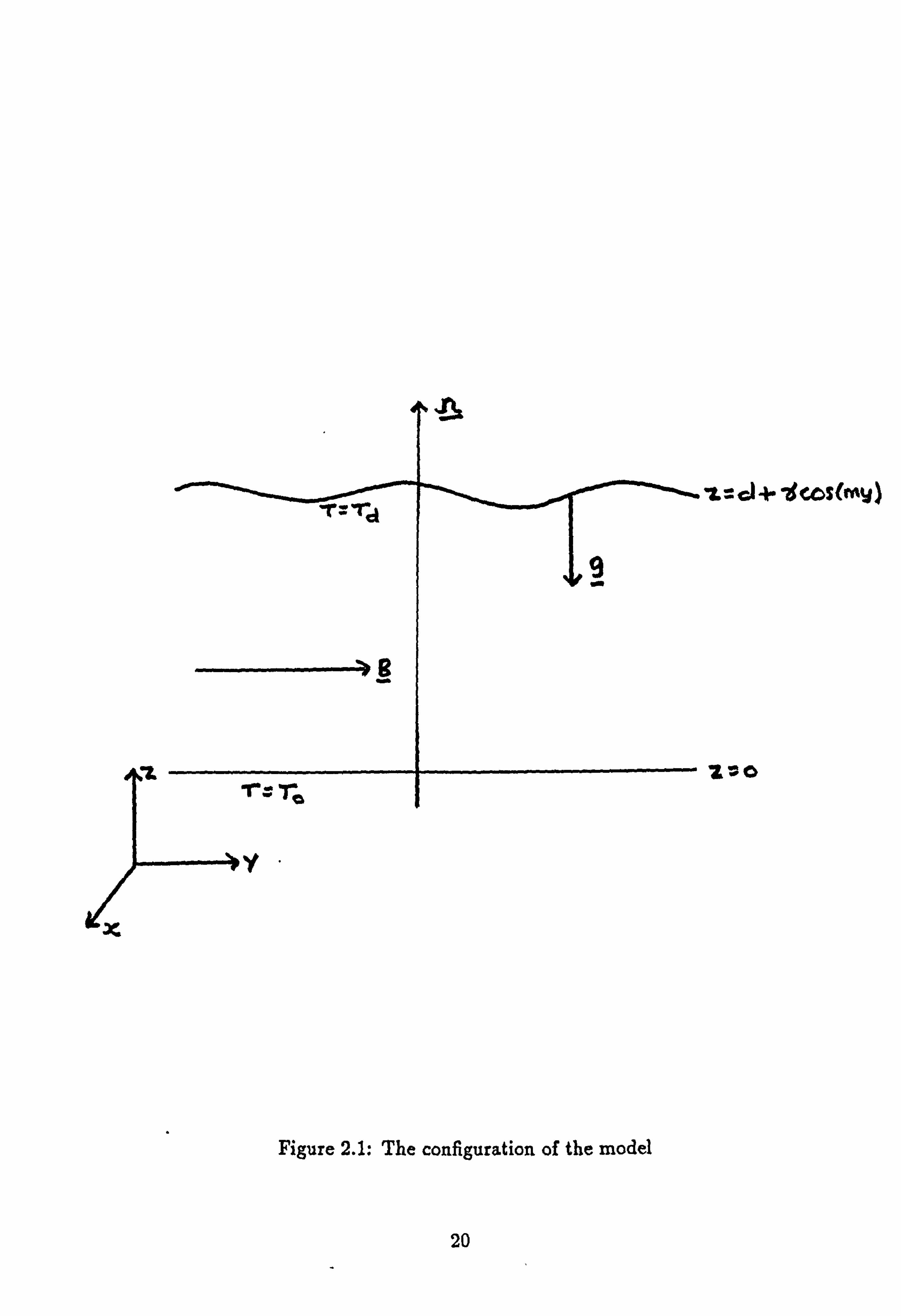
Z= cl -1- 7SCOS(r+rýyý
2O
r..
Figure 2.1: The configuration of the model
20

SZ = Slz, g= -gi, (2.4)
where SZ and g are real constants. This orientation of 0 and g corresponds to the
north polar region of the outer core, but the qualitative behaviour of the system is not altered by choosing arbitrary orientations (Chandrasekhar 1961).
Convection in the outer core is driven by a combination of thermal and com-
positional effects. As thermal convection is better understood and easier to model, all compositional effects will be ignored. In a thermally driven system, the bottom boundary is maintained at a constant temperature To and the top boundary is
maintained at a constant temperature Td. By choosing
To > Td,
the bottom boundary is made hotter than the top, and an adverse temperature
gradient
ßTO - Td >0,
is set up across the layer. This arrangement is unstable since hot, light fluid lies
beneath cold, heavy fluid. Convection ensues to restore the thermal equilibrium,
once the adverse temperature gradient becomes large enough.
The fluid in the layer is assumed to be Boussinesq - that is, temperature and
pressure variations across the layer are assumed to be sufficiently small that the density may be treated as a constant po everywhere, except where it appears with the buoyancy force. There, it takes the value
P= Po(1 - a(T - To)). (2.5)
The constant a is the coefficient of volume expansion, T is the temperature and To is the temperature at the bottom boundary. The fluid has kinematic viscosity v, thermal conductivity sc, magnetic permeability µp, electrical permitivity co and electrical conductivity a. For simplicity, all these quantities are assumed to be
constants. Note that in the core
21

v= 0(10-8),
so the effects of viscosity will be neglected over the bulk of the layer. Viscosity
is only important in thin, viscous Ekman layers that lie close to the bounding
surfaces.
2.2 The Boundary Conditions
It is assumed that the bounding surfaces are rigid, isothermal and perfectly electrically conducting. Now, these boundary conditions do not reflect the true
physics of the core. More accurate boundary conditions would reflect the fact that the lower mantle is (to a high approximation) electrically insulating, and not per- fectly electrically conducting. Similarly, a condition on the heat flux through the boundaries would be more realistic than arbitrarily imposing isothermal bound-
aries. However, of primary concern is isolating the mechanisms by which bumps
on the core-mantle boundary affect convection in the outer core. For this reason, these simpler, artificial boundary conditions are adopted to make the problem more tractable, in the hope that they retain all the essential physics of the problem.
These boundary conditions lead to conditions that the velocity U, temperature T, magnetic field B and electric field E must satisfy at the boundaries. To obtain these conditions, the normals to the boundaries are required. They are given by
z onz=0, n= (2.6)
z+ im sin(my)y on zd+ ry cos(my).
They are obtained by writing the boundaries in the form of a level surface
= constant,
so that the normals are given by
n=04.
22

2.2.1 The Boundary Conditions On The Velocity
At a rigid boundary, the velocity U satisfies
U. n = 0. (2.7)
This is the no penetration condition, which says that the fluid in the layer cannot penetrate into the regions outside of the layer. Using (2.6), the conditions at the bounding surfaces are, therefore
UZ =0 on z=0, (2.8a)
Uz+ 7m sin(my)Uy =0 on z=d -}- y cos(my). (2.8b)
Because viscosity has been neglected, the no-slip boundary condition on the veloc- ity (namely nAU= 0) does not have to be satisfied.
2.2.2 The Boundary Conditions On The Temperature
At an isothermal boundary, the temperature T satisfies
T= constant,
which says that the boundary is maintained at a constant temperature. Recalling that the bottom boundary is kept at a temperature To, while the top boundary is kept at a temperature Td, it follows that T must satisfy
T=To on z=0, (2.9a)
T= Td on z=d+y cos(my). (2.9b)
Note that To > Td, which sets up the adverse temperature gradient necessary to drive convection in the layer.
23

2.2.3 Electromagnetic Boundary Conditions
The regions outside the layer are perfectly electrically conducting. Hence
Q= oo in z<0, z>d+ -y cos(my).
However, the fluid in the layer has a finite electrical conductivity, so o- is finite in
the layer. This leads to a discontinuity in o at the boundaries. At a boundary
where o is discontinous, the magnetic field B and the electric field E must satisfy
[B. n]=0, [nAE]=0,
where the square brackets denote the jump in value across the boundary (see
Gubbins and Roberts in Jacobs 1987). Ignoring any electromagnetic fields outside the layer, B and E must satisfy
B. n=0, nAE=0 on z=0 and z=d+ycos(my). (2.10)
Now, using Ohm's law, the boundary condition on E can be replaced by an
equivalent condition on the electric current, J= µo (0 A B). Ohm's law is
1J=E+UAB.
CT
Taking the cross product with n and using a standard vector identity, this becomes
nAJnAE+ (n. B)U - (n. U)B. (2.11)
Using (2.7) and (2.10) this says that
nAJ=O on z=0 and z=d+rycos(my). (2.12)
Therefore, an equivalent set of boundary conditions is
24
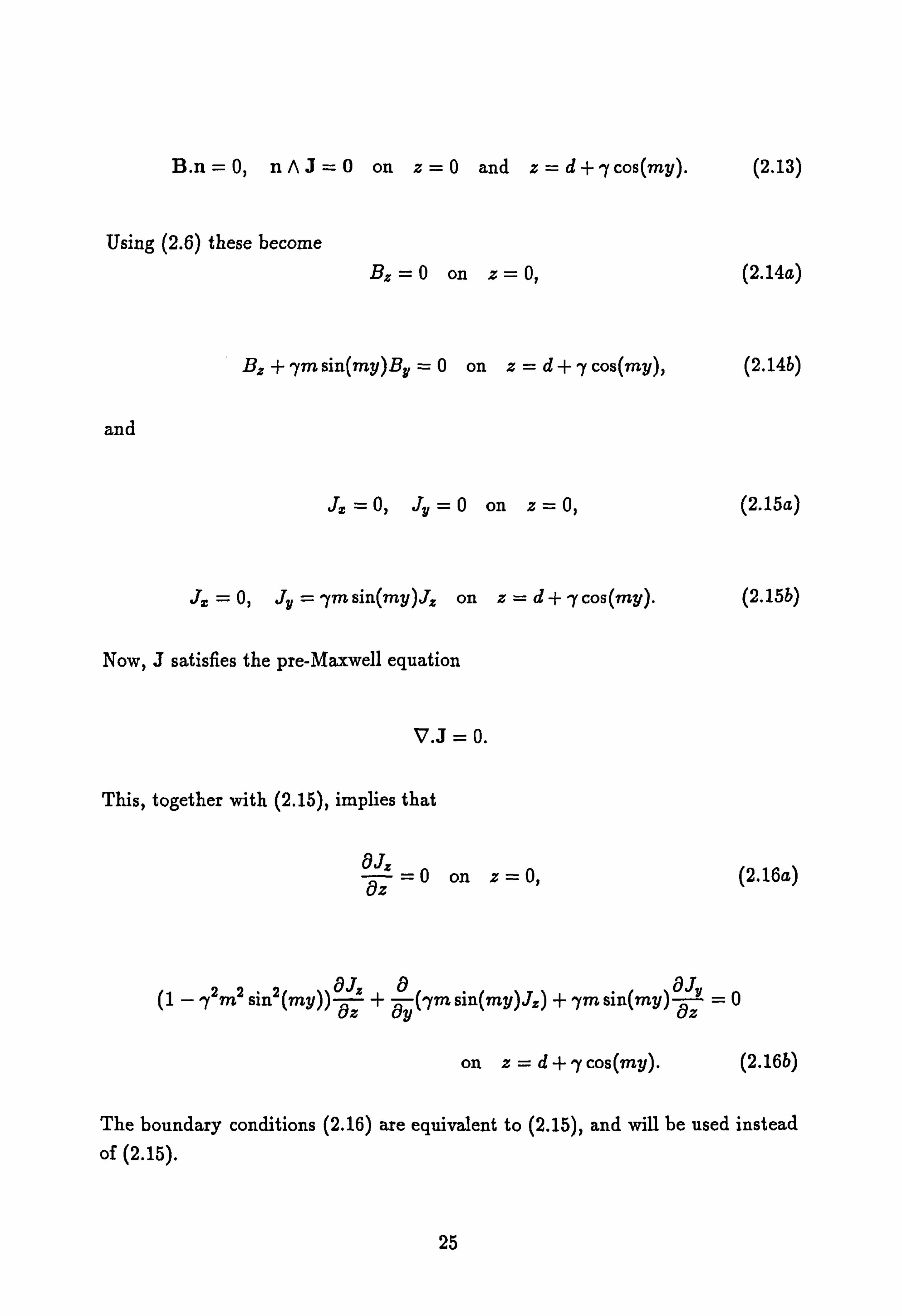
B. n=0, nAJ=O on z=0 and z=d+rycos(my). (2.13
Using (2.6) these become BZ=O on z=0, (2.14a)
Bz+ rym sin(my)BV =0 on z=d+y cos(my), (2.14b)
and
J. =O, Jy =0 on z=0, (2.15a)
J, =O, Jy= 7m sin(my)JZ on z=d+ -y cos(my). (2.15b)
Now, J satisfies the pre-Maxwell equation
v. J=o.
This, together with (2.15), implies that
oJz
Oz =0 on z=0, (2.16a)
(1 - yzm2 sin2(my)) j,
+y (-/m sin(my)J-. ) + -/m sin(my) azy
=0
on z=d+ ry cos (my). (2.16b)
The boundary conditions (2.16) are equivalent to (2.15), and will be used instead
of (2.15).
25

2.2.4 Taylor Expansion Of The Boundary Conditions
The boundary conditions on the surface z=d+ ry cos(my) are very difficult to apply. However, it is possible to obtain a simpler set of boundary conditions, which (hopefully) retain all the essential features, but which are applied on z=d. This is done by Taylor expanding the full set of boundary conditions in -y, using the fact that 7«1, retaining only 0(1) and 0(y) terms. This yields the conditions
Uz=Q BZ_0 gJ on z=0, (2.17a)
, 9--L 0
To
UU + ry cos(my)jýL = -rym sin(my)UU
eý eZJ _BZ
e ry cos(my) --fm sin(my)By on z=d.
-= -ý-Y(rym sin(my)J-. ) - -Im sin(my)- fr -{- -Y Cos (my)
T+ ry cos(my) ez = Td
(2.17b)
This idealised set of boundary conditions will be applied instead of the full set. However, any effects caused by their imposition will be attributed to the bumps.
2.3 The Equations
The equations that the system must obey are derived from the various phys- ical laws that govern a rotating, Boussinesq fluid in the presence of a magnetic field. The first law is Newton's law of motion, which is used to derive the mo- mentum equation. Now, to model motion in the core, the magnetogeostrophic approximation is made, and the magnetogeostrophic equation is obtained
211 AU= -V(P) +1 (B. 0)B +Pg, (2.18a) Po Popo Po
where
26

P= Po(1 - a(T - To)), (2.18b)
P=P-1PoIflAxj2+ 1 Bz (2.18c) 2 2µo
are the density and modified pressure respectively. The left hand side of (2.18)
represents the Coriolis force, while the right hand side represents the pressure force, the Lorentz force and the buoyancy force respectively. Recall from chapter 1 that the fluid velocity U cannot be determined uniquely from (2.18). It can only be determined up to an arbitrary flow, V(x)y called the geostrophic flow. This
arbitrariness arises as a consequence of the magnetogeostrophic approximation. To determine V, and hence find the flow velocity uniquely, the following equation
must be solved
2(Sty)"V =1 8M
(2.19a) µo po äx '
where
2d M=
2d Joi j B. Bydzdy, (2.19b)
is the mean Maxwell stress in the y direction (see Soward 1980; Soward and Jones
1983; Abdel-Aziz and Jones 1987). Equation (2.19) represents conservation of mass in the x direction, but includes contributions from the viscous Ekman layers
that lie at the boundaries. (This is the only place in the model where the effects of
viscosity are important). The second law is conservation of mass. This is embodied in the continuity equation,
V. U = 0. (2.20)
The first law of thermodynamics yields the heat equation
OT + (U. V)T = ý, V2T. (2.21)
27

The left hand side of (2.21) represents advection of heat by the fluid, while the
right hand side represents the removal of heat by thermal diffusion. The laws
of electrodynamics (namely Faraday's law, Ohm's law and Ampere's law) can be
combined to give a single equation for the magnetic field. This is the induction
equation, which is given by
1B + (U. V)B = (B. V)U + 77V2 B, (2.22)
where
1 71_ , 1Lo0
is the magnetic diffusivity. The left hand side of (2.22) represents advection of the field by the flow, while the right hand side represents stretching of the field lines
by the motion of the fluid, and destruction of field by Ohmic diffusion. Finally, B
satisfies a solonoidal condition
V. B=o. (2.23)
This equation arises because magnetic monopoles do not exist in nature. Hence,
the flux of B through any closed surface must be zero.
2.4 The Formulation Of The Problem
The equations are nondimensionalised by adopting the following scalings
x= Dx*, t= Tt*, (2.24a, b)
1 y= Dy*, M= 5m*, (2.24c, d)
O. V* (2.24e)
28

where the starred quantities are nondimensional, and
E)2 D=-, T=D
,
have been adopted as length and time scales repectively. As is common in convec- tion problems, time has been scaled on the basis of the thermal diffusion timescale. The velocity, magnetic field and temperature scale as follows
U= D(V *(x)Y +'y' ü*)ý (2.25a)
B= Bo(Y + 7*Qb*), (2.25b)
T= , QD(TT - z* + ry*b*), (2.25c)
where q is the Roberts number.
The flow V*(x)y is the geostrophic flow that arises as a consequence of the
magnetogeostrophic approximation, but it is corrected by a flow ry*u*, which is
determined to ensure that the geostrophic flow fits into a layer with a bumpy top boundary. The form of the geostrophic flow arises for the following reason. The
true geostrophic flow in the bumpy layer takes the form U*(x, y, z)y. Consider the
mass flux across the plane y=Z, at which the layer has height 7r. It is given by
. *F=7rU*(x, 2) r)'
This mass flux J must be the same as the mass flux across any arbitrary plane
y= yo, at which the layer has height zo =7r + y* cos(m*yo). Hence,
.ý= aU*(x, 2,7r)
= (7r + -y* cos(m*yo))U*(x, yo, , zo).
Defining V*(x) = U* (x, Z, ir) the following relation is obtained
29
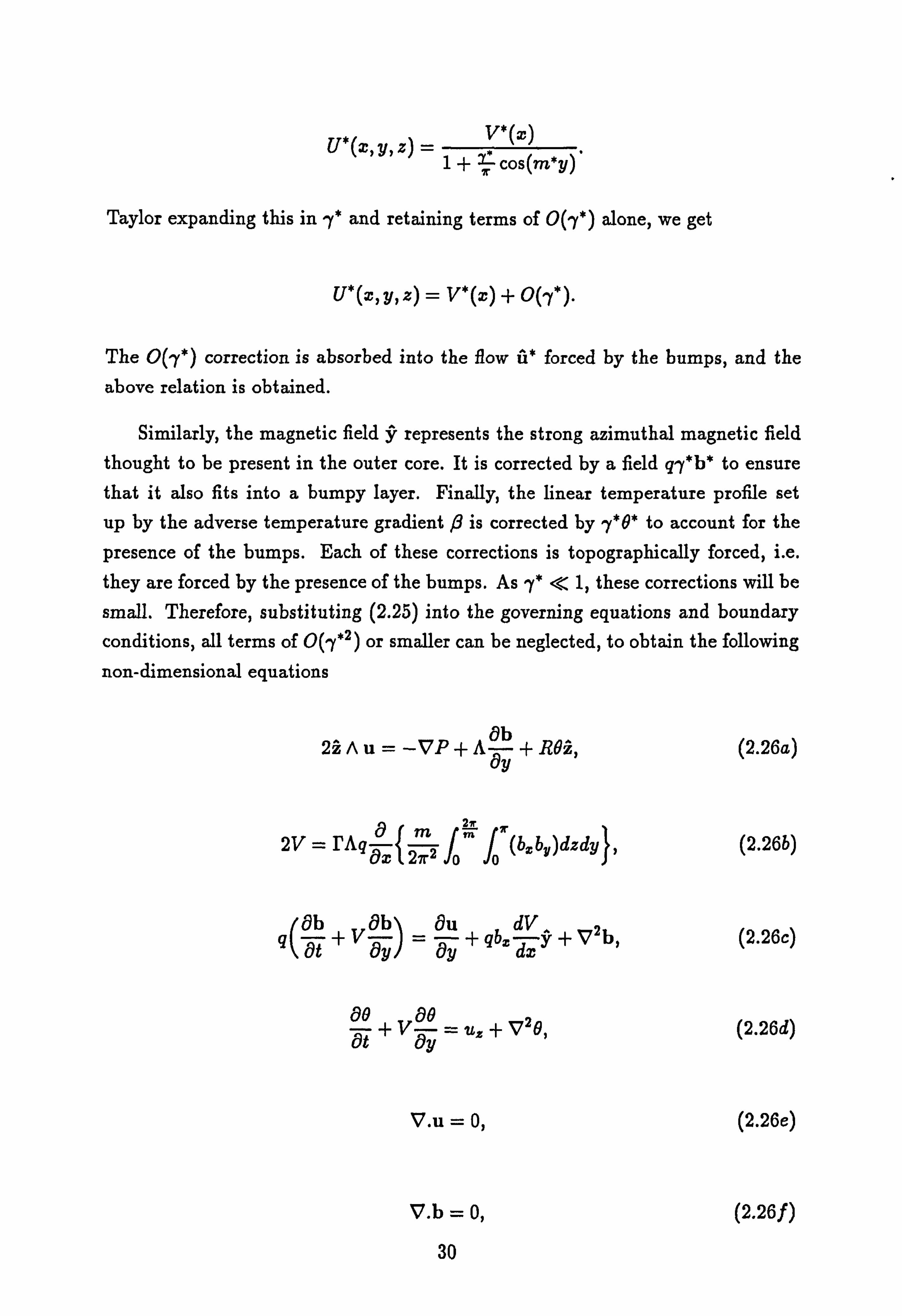
U*(X, y, z) =1+ 21 cosým*y)
Taylor expanding this in ry* and retaining terms of 0(ry*) alone, we get
U*(ýýyýz) = v* (x) + 0(7*).
The 0(7*) correction is absorbed into the flow it forced by the bumps, and the
above relation is obtained.
Similarly, the magnetic field y represents the strong azimuthal magnetic field
thought to be present in the outer core. It is corrected by a field qy*b* to ensure that it also fits into a bumpy layer. Finally, the linear temperature profile set up by the adverse temperature gradient ß is corrected by y*9* to account for the
presence of the bumps. Each of these corrections is topographically forced, i. e. they are forced by the presence of the bumps. As ry* « 1, these corrections will be
small. Therefore, substituting (2.25) into the governing equations and boundary
conditions, all terms of 0(, y*2) or smaller can be neglected, to obtain the following
non-dimensional equations
2zAu= -VP +A Ob
+ RO , (2.26a)
y
r 2r
m (bxby)dzdy}, (2.26b) 2V = rAgOx { 27r2 mff
q(Ob +V 0b)
= On
+ qbx dV
Y+ V2 b, (2.26c)
ae ae _ Ft + vöy ' uz + v2o, (2.26d)
V. u = 0, (2.26e)
V. b = 0, (2.26f)
30
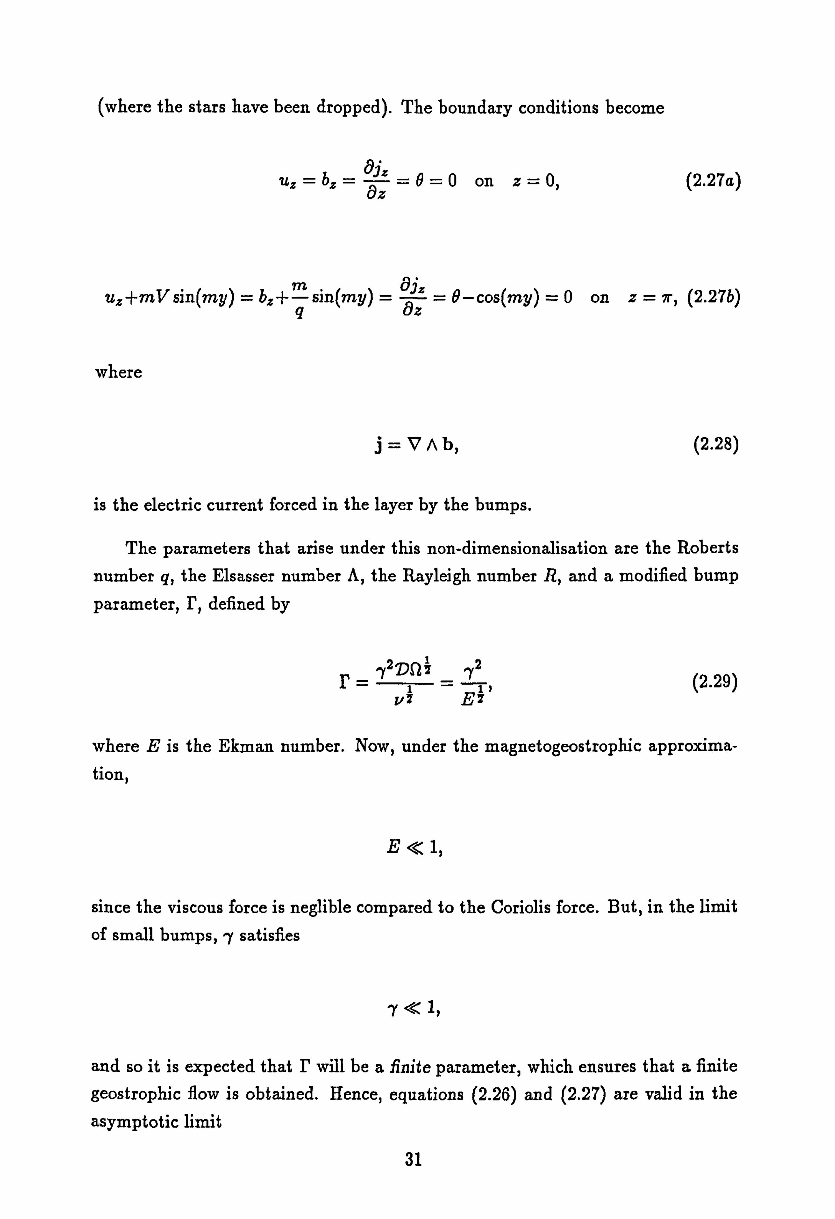
(where the stars have been dropped). The boundary conditions become
uz bz -- 19 ajz =0=0 on z=0, (2.27a)
uz+mV sin(my) = bz+ m sin(my) = 'ýz = 9-cos(my) =0 on z= 7r, (2.27b)
where
j=V Ab, (2.28)
is the electric current forced in the layer by the bumps.
The parameters that arise under this non-dimensionalisation are the Roberts
number q, the Elsasser number A, the Rayleigh number R, and a modified bump
parameter, r, defined by
r_ ry2Dý2l _1 (2.29)
V'2 E-
where E is the Ekman number. Now, under the magnetogeostrophic approxima- tion,
E<11
since the viscous force is neglible compared to the Coriolis force. But, in the limit
of small bumps, ry satisfies
7 4Z 1,
and so it is expected that r will be a finite parameter, which ensures that a finite
geostrophic flow is obtained. Hence, equations (2.26) and (2.27) are valid in the
asymptotic limit
31
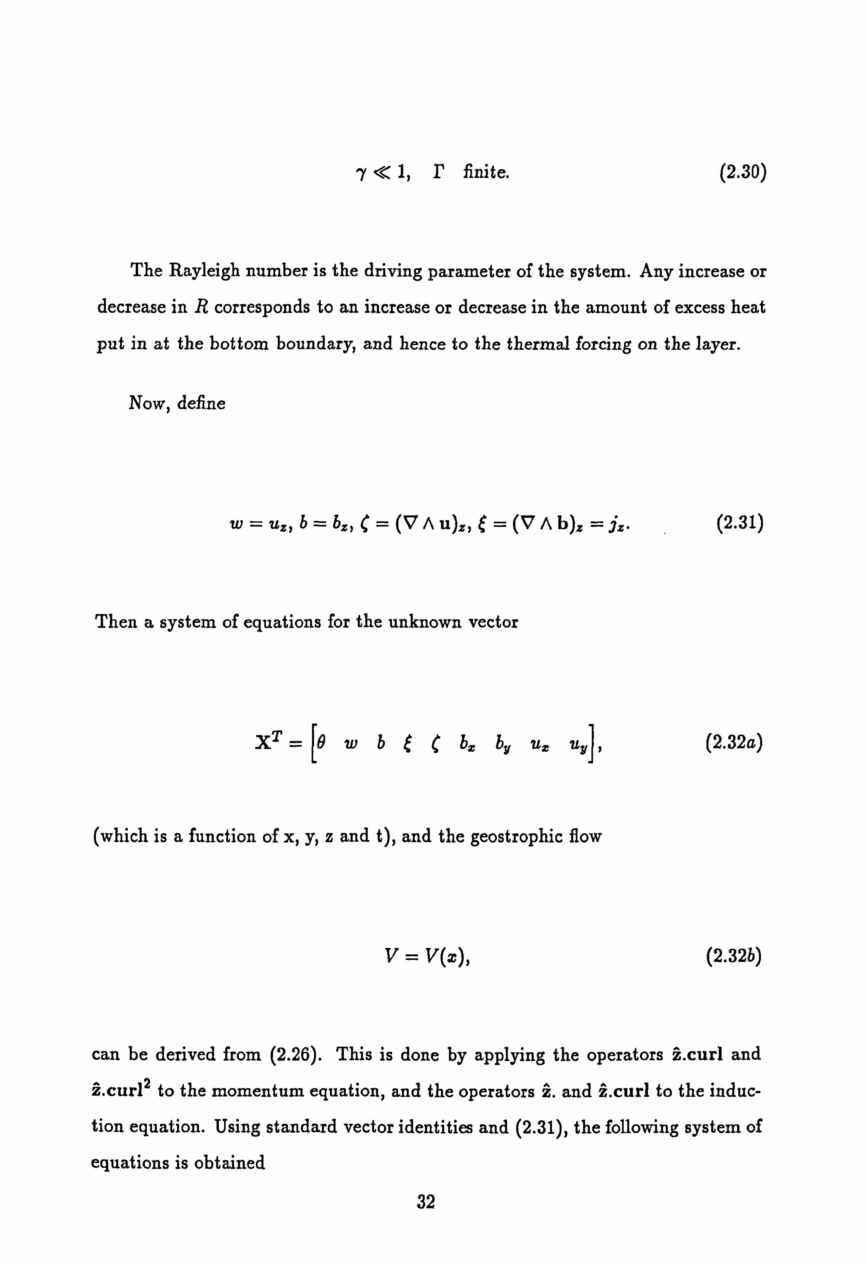
y«1, r finite. (2.30)
The Rayleigh number is the driving parameter of the system. Any increase or
decrease in R corresponds to an increase or decrease in the amount of excess heat
put in at the bottom boundary, and hence to the thermal forcing on the layer.
Now, define
w= uz, b=bz, C=(VAU)Z, ý=(VAb), z=iz. (2.31)
Then a system of equations for the unknown vector
XT = [B
wbýC bx by ux uyII (2.32a)
(which is a function of x, y, z and t), and the geostrophic flow
V= V(x), (2.32b)
can be derived from (2.26). This is done by applying the operators a. curl and
2. cur12 to the momentum equation, and the operators z. and z. curl to the induc-
tion equation. Using standard vector identities and (2.31), the following system of
equations is obtained
32
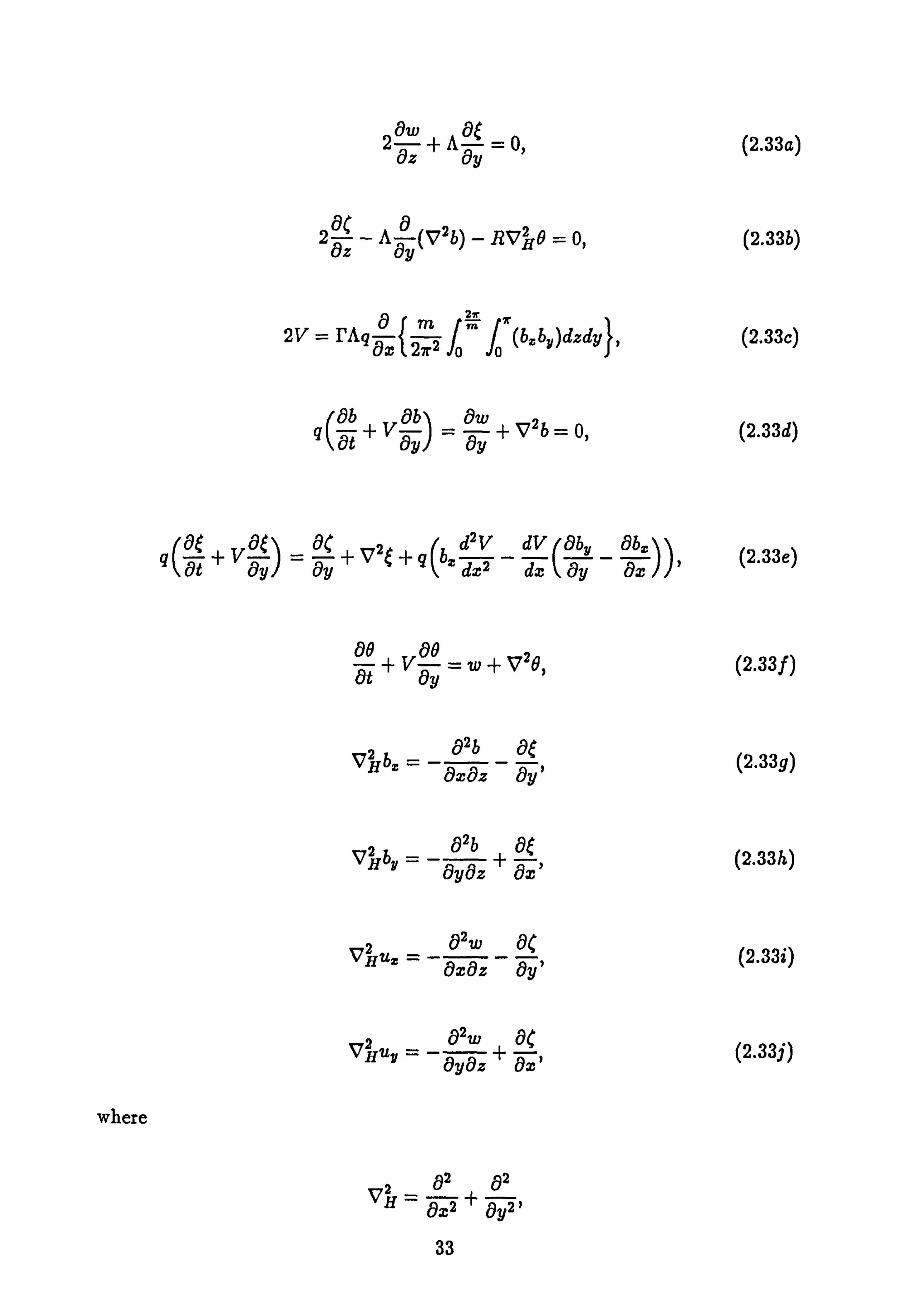
2 ýz
+A=0, (2.33a) y
2clz -A 19
(V2b) - RV JO = 0, (2.33b)
r 2, r
2V = PAqý { 2ý2 f '" f (bxby)dzdy}, (2.33c)
(fit +V _) _
ýy + V2b = 0, (2.33d)
(Lb 4(a `f' V
ciy) = äy V2 +q (bý, ax dV
äyß öx )), (2.33e)
00 + v00 =w+ V29, (2.33f) y
VHb ,2a äz äy, (2.33g)
ab a) ýHbý ayaz + aX'
2.33h
°Hux ̂ Ozaz - ay, (2.33i)
V2 02w O
where
a2 a2 Ox = äx2 -f 8y2 l
33

is the horizontal Laplacian operator. (Note that the solenoidal conditions on u and b have been used together with the definitions of ý and C to derive the last four equations of (2.33)). Using (2.31) the boundary conditions become
w=b=az-B_0 on z=0, (2.34a)
w+ mV sin(my) =b+q sin(my) _=0- cos(my) =0 on z= ir. (2.34b)
Equations (2.33) will be solved subject to (2.34) in the subsequent chapters.
2.5 A Note On The Choice Of q And m At various points in this work, it will be necessary to make choices for the
values of the parameters q and m. In the core, the value of q is thought to be 0(10-6). This is an extremely small value, and as the work of Soward (1986) and Skinner and Soward (1988,1990) shows, the behaviour of solutions of the mag- netoconvection problem is extremely complicated in the small q limit. However,
since this work is chiefly concerned with isolating the effects of the topography
upon the magnetoconvection, it is necessary to isolate those effects from any that
might arise as a result of the smallness of q. Hence, this work will not consider small values of q.
Now, the value of m for the core is not known, and therefore it would be
advisable to solve the problem over a range of values of m. However, the results of Kelly and Pal (1977) indicate that the critical values of m that arise in the standard plane layer model give rise to the most interesting behaviour in the bumpy layer,
since the possibility of resonance between the bumps and the convection in the layer then arises (see also chapter 4 for more details). Therefore, as a matter of expediency, the values of m will be chosen to be the critical values of m that arise in the standard layer, since these appear to give the most interesting behaviour in the bumpy layer. However, the observation that these are but one out of a continuum of values of m should be borne in mind when considering the results of this work.
34
Chapter III
The No Bump Case
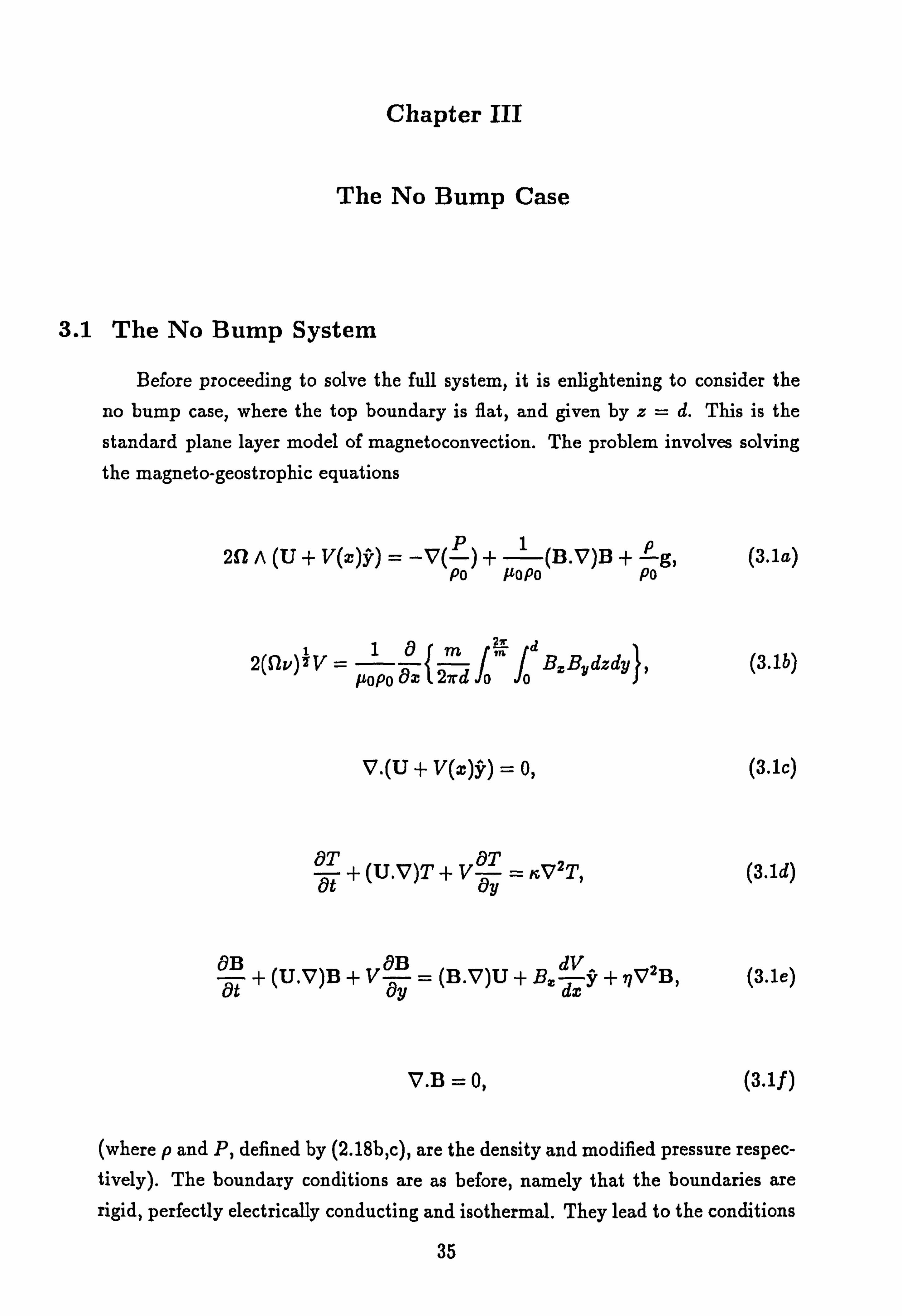
3.1 The No Bump System
Before proceeding to solve the full system, it is enlightening to consider the
no bump case, where the top boundary is flat, and given by z=d. This is the
standard plane layer model of magnetoconvection. The problem involves solving the magneto-geostrophic equations
21 A (U + V(x)Y) = -V(P) +1 (B. V)B + -f-g, Po Popo Po
Z* dl 2(Stv)' V=
1 a{ mfmfB., Bdzdy }, (3.1b) µoPo ax 2ýrd ooJ
V. (U + V(x)y) = 0, (3. lc)
at + (U. V)T +v ay = , ýV2T, (3. ia)
OB + (U. V)B -4- V -äy = (B. V)U + Bx
dx g+ 7lV2B, (3.1e)
V. B=o, (3.1 f)
(where p and P, defined by (2.18b, c), are the density and modified pressure respec- tively). The boundary conditions are as before, namely that the boundaries are rigid, perfectly electrically conducting and isothermal. They lead to the conditions
35
Uz Bs Oz, _T-To-O on z=0, (3.2a)
UZ BZ azx =T-Td=0 on z=d. (3.2b)
In the no bump case, these boundary conditions are exact.
3.2 The Equilibrium Solution
A steady solution of (3.1) subject to (3.2) is
U=0, (3.3a)
V=0, (3.3b)
B= Boy, (3.3c)
T= To -, ßz. (3.3d)
This is the hydrostatic conduction solution, so called because the fluid in the layer
remains at rest, and excess heat at the bottom boundary is carried across the layer by thermal diffusion (Chandrasekhar 1961). Such a motionless solution is possible because the equation of hydrostatic equilibrium is satisfied,
VP + pgz = VP + po(1 - a(T - To))gz = 0.
Taking the curl of this equation yields
VTAZ=0, (3.4)
36
which says that the surfaces of constant temperature (isotherms) are horizontal. This is the condition that ensures that a hydrostatic balance is possible in a plane layer.
3.3 The Perturbation Equations
To see how motion develops from the hydrostatic basic state, the stability of (3.3) must be considered. This is done by adding small perturbations to U, B
and T and asking whether the perturbations grow or decay with time. If the
perturbations decay, then motion does not become established in the layer, and the basic state (3.3) is said to be stable. If, however, the perturbations grow in time, then motion does become established in the layer and (3.3) is said to be
unstable. Denoting the perturbations by u, b and B, the velocity, magnetic field
and temperature take the the following form in the perturbed state
U= D(0 + Su*), (3.5a)
B= Bo(Y + bqb*), (3.5b)
T= ßD(TT - z* + 66*), (3.5c)
where q is the Roberts number (defined by (1.1)), b«1 is a small parameter mea- suring the size of the perturbations, and the starred quantities are nondimensional. The unknowns have been nondimensionalised by adopting
D-a, D2 T=-
as length and time scales, respectively. Substituting (3.5) into (3.1) and (3.2), and neglecting all terms of 0(52) or smaller, the nondimensional equations governing departures from hydrostatic equilibrium are obtained. These are given by
37

b+ RBz, (3.6a) 2z Au= -VP +A äy-
V. u = 0, (3.6b)
ae = uz + v2e, (3.6c)
at
Ob au 2 q ýt - ýy +Ob, (3.6d)
v. b _ a, (3.6e)
where here and below the stars are dropped. As well as the Roberts number q, the
other parameters of the problem are A, the Elsasser number and R, the Rayleigh
number. Note that
bxby = 0(52),
so no Maxwell stress is generated at 0(5), and hence, no geostrophic flow is ac-
celerated by the perturbations. The boundary conditions on the perturbations
are
z uZ - bz äj7 -0=0 on z=0, ir,
where j=VAb is the perturbation electric current. Define
w=u,, b=bz, C=(VAu)Z, ý=(VAb), z=. 7=.
Then, exactly as in chapter 2, a system of equations for the vector
XT = [B
wbeC bx by u uy1,
38

may be derived from (3.6). They are
2 ýz
+ Ae- = 0, (3.7a) y
2iz - A-y(V2b) - RV 2=0, (3.7b)
ab w a-vz y b=0, (3.7c)
A- -
ay - V2e = 0, (3.7d)
09 ät -w-V 2B = 0, (3.7e)
°Hbx - -O 2
az b-
ýy, (3.7f)
N72 U aylb
aý °A =- oz + äx, (3.7g)
2 02w OC
VHUZ axaz - ey, (3.7h)
V2 52w 5ý
U
39

where V is the horizontal Laplacian. The boundary conditions become
w=b= ý
=8=0 on z=0 and z=ir. (3.8) c9z
3.4 Solutions Of The Perturbation Equations
The solutions of (3.7) and (3.8) must be periodic in x and y, with periods T T- and respectively. To satisfy this condition, a solution of (3.7) and (3.8) is sought of the form
X= Xi(z) exp(ilz + imy + At) + c. c., (3.9)
where
Xi '(z) _ [Ti(z) Wi(z) Bi(z) X, (z) Z, (z)
B,, l(z) Byl(z) Uxl(z) Uyi(z),, (3.10)
represents the z-structure of (3.9) and c. c. stands for complex conjugate. (The
reason for including a subscript 1 will be made clear later). A is a complex number defined by
A=3+iw, (3.11)
where s is the growth rate and w is the frequency of the perturbations. (3.9)
represents a convection roll, whose axis is perpendicular to the vector defined by
k- (l, m, 0).
Two distinct types of roll can arise, depending on their orientation with the applied magnetic field (which is in the y direction). A solution which has l 74 0 is called an
40

oblique roll, since it's axis makes an angle less than 2 with the applied magnetic field, and a solution which has I=0 is called a transverse roll, because it's axis is perpendicular to the applied magnetic field. Although the transverse roll is a special case of the oblique roll, it has different stability characteristics, and will be
discussed in isolation.
Substituting (3.9) into (3.7) the equations for the z-structure of the roll are
obtained. These are given by
2DW1 + AimX1 = 0, (3.12a)
2DZ1 - Aim(D2 - k2)B1 + Rk2T1 = 0, (3.12b)
(D2 - k2 - ga)Bi + imW1 = 0, (3.12c)
(D2 - k2 - ga)Xi + imZi = 0, (3.12d)
(D2 - kz - A)T1 + Wi = 0, (3.12e)
k2Bz1 - iLDB1 - imX1 = 0, (3.12f)
k2By1 - imDB1 + ilXj = 0, (3.12g)
k2UZ, - ilDW1 - imZi = 0, (3.12h)
k2Uyl - imDW1 + ilZ1 = 0, (3.12i)
where here and below
41
d
k2=12-ßm2"
Substituting (3.9) into (3.8) the boundary conditions become
Wi=Bl=DX1=Ti=0 on z=0 and z=zr.
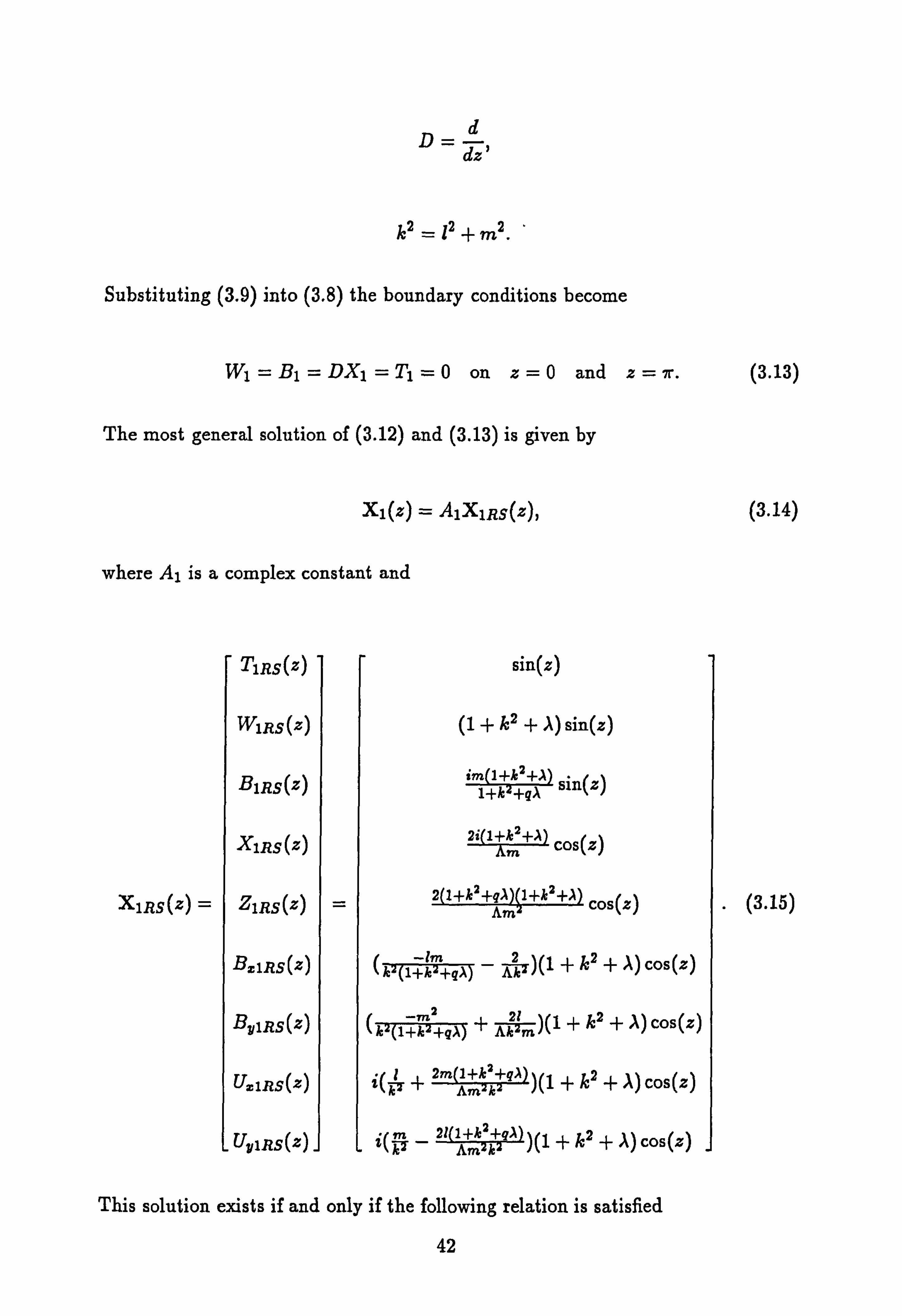
The most general solution of (3.12) and (3.13) is given by
Xl(z) = A1X1RS(z),
where Al is a complex constant and
T1RS(z)
W1RS (z)
B1RS(z)
X1RS(z)
X1RS(z) = Z1RS(z) _
Bz1RS(z)
By1RS (z)
Ux1RS(z)
Ug1RS(z)
sin(z)
(1-i-k2+A)sin(z)
im 1+k2+. a sin(z) 1+k +qa
2i 1+k2+. Am cos(z)
2(1+k2+qa)(1+k2+a) cos(z) Am4m
(k 1+k +qa - Ak9)(1 + k2 + . 1) cos(x)
2
qa +Aß)(1 + k2 + A)cos(z) (k
1+k +
Z(k + 2m Amkk+qa )(1 + k2 + a) COS(z)
i(m _ 2t 1+kak a)(1 + k2 + A) cos(z)
(3.13)
(3.14)
I. (3.15)
This solution exists if and only if the following relation is satisfied
42

4(qA +1+ k2)2(A +1+ k2) + A2m4(A +1+ k2)(1+ k2)
-k2Am2(ga +1+ k2 )R = 0. (3.16)
(3.16) is called the dispersion relation. The real and imaginary parts of (3.16) give two equations for the two unknowns s and w. For fixed values of A and q, the solution of these two equations takes the form
s= s(R, 12, m2), w= cu(R, 12, m2)
The stability of the basic state (3.3) depends upon the sign of 3. If at given values of R, landm
3(R, 12, m2) < 0,
then the perturbations will decay exponentially in time to leave the basic state as it was. Hence, (3.3) is stable. However, if
s(R, 12, m2) > 0,
then the perturbations will grow exponentially in time, and the basic state will lose stability to the convection roll defined by (3.9). Hence, (3.3) is unstable. The
point at which the basic state loses stability for given A and q is defined by
s(R, 12, m2) =
Now, this defines a relation of the form
R= R(lz, m2), (3.18)
i. e., for given values of l and m it defines the Rayleigh number at which the basic
state (3.3) goes unstable to perturbations of the form (3.9). To find where this first occurs, (3.18) must be minimised with respect to 12 and m2. This is done by
solving the simultaneous equations
43

OR OR äl2 8m2 - 0.
These yield the critical wavenumbers 1, and m, for which R defined by (3.18) is a minimum. This is the critical Rayleigh number, and is defined by
R, = R(lc2, m').
The basic state is stable to the perturbations for R<R,, but loses stability to the perturbations at R=R,. The frequency of the perturbations at criticality is
given by
wc c2 zý =w Rc, l,, m,.
For the transverse rolls, the above procedure is repeated, but with I set to zero.
3.5 Linear Stability Results
The stability results quoted below were first derived by Roberts and Stewartson (1974). Now, R, and w. can be found directly from (3.16) by setting
s-0,
in (3.16). This yields
4(giw+1 +k2)2(iw+1+k2)+A2m4(iw+1 +k2)(1+k2)
-k2Am2(giw +1+ k2)R = 0. (3.19)
The real part of (3.19) is
(1 + k2) [4q(q + 2)w2 - {4(1 + k2)2 + A2m4(1 + k2) - k2Am2R}] = 0, (3.20)
44
while the imaginary part is
w[4g2w2 - {4(2q -x-1)(1 + k2)2 +A 2M4(1 + k2) - k2 Am2qR}] = 0. (3.21)
These provide two equations for the two unknowns R and w, from which R, and we can be found.
3.5.1 The Exchange Of Stabilities
The simplest solution of (3.21) is
w2 = (3.22)
This means that the basic state loses stability to steady perturbations, which is
called losing stability through the exchange of stabilities (Chandrasekhar 1961).
Substituting (3.22) into (3.20) gives
R= 4(1 + k2)2
+ Am2(1 + k2) (3.23)
Am2k2 k2
The critical wavenumbers l, and m, are found from the simultaneous equations
OR 0R äl2 amz = o.
The solution of these equations is given by
2ý 2/ lc =2-A, me -A (3.24)
Evaluating (3.23) on these values yield the critical Rayleigh number for an oblique roll
Rý=Nr3i. (3.25)
45
Thus, as R is increased from zero, the basic state first loses stability to an oblique
roll (whose wavenumbers are given by (3.24)) through the exchange of stabilities
once R equals Rc. This result depends upon the value of A: if
<-43,
then
lc < 0,
which cannot happen, since d is real. Therefore, the oblique roll can only go
unstable for sufficiently strong magnetic fields, those which satisfy
A> -vF3. (3.26)
Setting l=0 in (3.20) yields R for the transverse roll
= 4(1 + m2)2 R Am4 -F A(I + M2). (3.27)
The critical wavenumber m, for this roll is defined by the solution of
OR äm2
that is, as the solution of
A2m6 - 8(1 + m2) = 0. (3.28)
(3.28) is regarded as a cubic equation for m2, and m2 is chosen to be it's positive
root. Evaluating (3.27) on mc yields the critical Rayleigh number for the transverse
roll
_ 4(1+m)2
Rc Am4 +A(l+m'c),
c 46
10
8
6
A 4
2
0
q
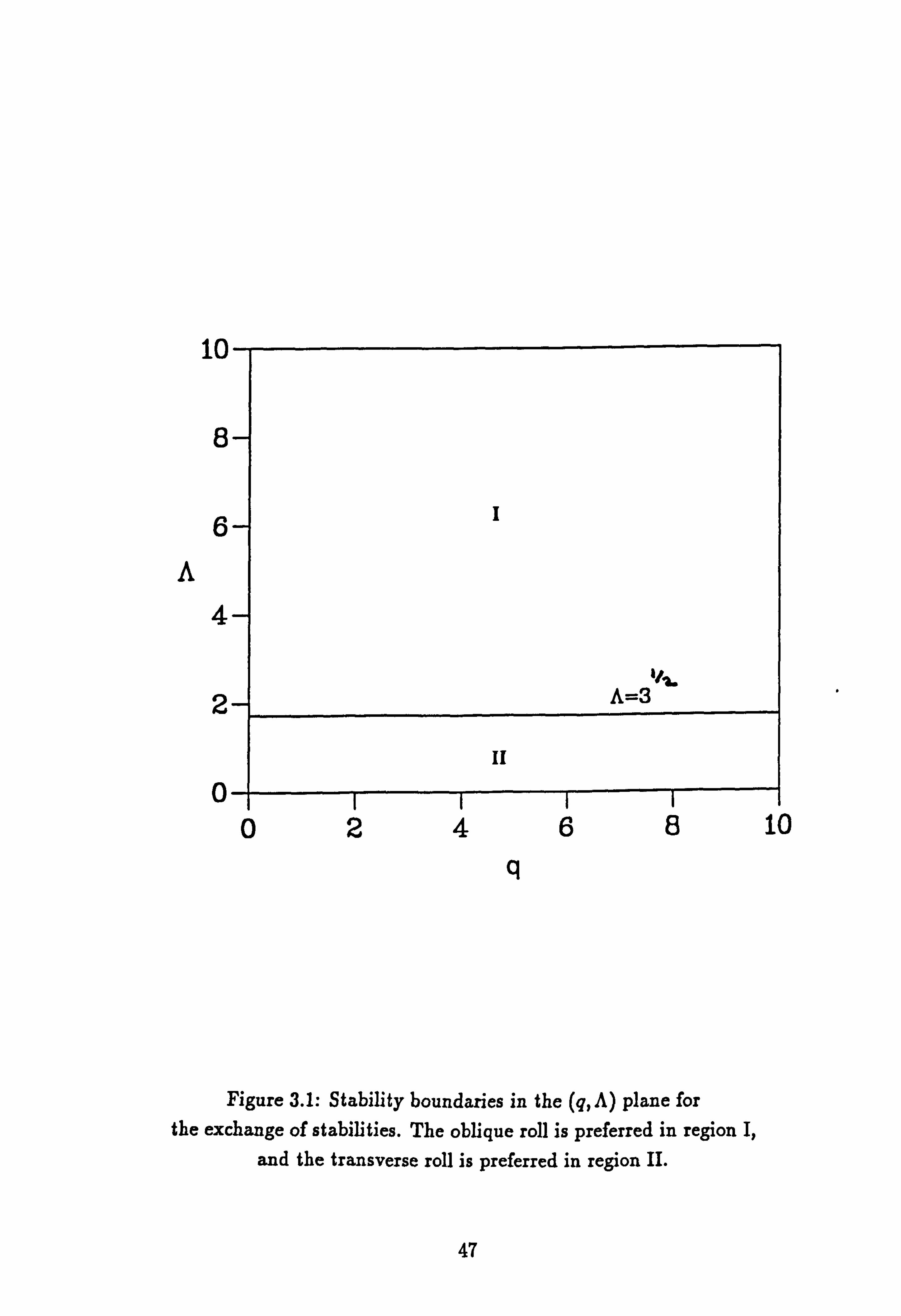
Figure 3.1: Stability boundaries in the (q, A) plane for the exchange of stabilities. The oblique roll is preferred in region I,
and the transverse roll is preferred in region II.
47
02468 10

which after simplifying using (3.28) becomes
Rc 2(2+m2)(1+m2).
(3.29)
Thus, as R is increased from zero, the basic state first loses stability to a transverse
roll (whose wavenumber is given by mc) through the exchange of stabilities when R equals R,. This occurs for all values of A.
Now, when A>/, the basic state can lose stability to either a transverse roll
or an oblique roll. It actually loses stability to only one - the one with the lowest
critical Rayleigh number. This roll is then said to be preferred for A> A/3. Since
6/ is the minimum of
_ 4(1-I- k2)2 Am2(1 + k2)
R Am2k2 + k2
over all I and m, including the case 1=0, it follows that the oblique roll has a lower critical Rayleigh number that the transverse roll, and is the preferred mode
of convection for A>3.
Hence, for weak magnetic fields, i. e. those satisfying
n<ý,
the basic state loses stability to a transverse roll through the exchange of stabilities. But, once the magnetic field strength (as measured by A) increases beyond /,
the oblique roll becomes preferred, and the basic state loses stability to an oblique
roll through the exchange of stabilities. This is shown in figure 3.1.
3.5.2 Overstability
The second solution of (3.21) is
2= 4(2q -I-1)(1-ß k2)2 + A2 4q2
m4(1 + k2) - k2Am2gR w_ (3.30)
Now, w is real, so
48
w2>0.
When this holds (and conditions will be found to ensure that it does) the basic
state loses stability to perurbations that oscillate with frequency w. This is called losing stability through the mechanism of overstability (Chandasekhar 1961). Sub-
stituting (3.30) into (3.20) and simplifying yields
R_2(4(1+kz)z+Amz(1-+ - kz)\ 3.31
4l Amzkz k2 )' )
where
ÄA = 1+q, (3.32)
is a modified Elsasser number. Substituting (3.31) into (3.30) and simplifying yields
w2 = (q2 - 1)Ä2m4(1 + k2) - 4(1 + k2)2
(3.33) 4q2
The critical wavenumbers minimising R are found from the simultaneous equations
OROR_ 012 _ äm2
The solution of these equations is given by
P=2-2 (1 + 4), me = 2A (1 + q). (3.34)
Evaluating (3.31) and (3.33) on these values yields the critical Rayleigh number and the frequency of the oblique roll, which are given by
Rc = 12vf3- (3.35)
q
49

we = 9(92 Z 2). (3.36)
9
Therefore, as R is increased from zero, the basic state first loses stability to an
oblique roll (whose wavenumbers are given by (3.34)) through overstability once R
equals R,. The frequency of the perturbations at criticality is given by w,. Notice
that we is real only when
Q> _V"
Similarly, 1, is real only when
A>Al(q) =V(1+q)"
Thus, an overstable oblique roll is only possible in the region of the (q, A) plane defined by
q>V, A> Ai (q), (3.37)
since only in this region are both w, and 1, real.
Setting l=0 in (3.31) and (3.33) yields the Rayleigh number and the frequency
associated with the transverse roll
Rq2 (4(1Äm4 2)2
+ Ä(1-i- m2)), (3.38)
2- (q2 -1)Ä2m4(1 + m2) - 4(1 + m2)2 (3.39) 4q2
The critical wavenumber minimising R is found from the solution of
OR äm2 = 0,
i. e. from the solution of
50

A2m6 - 8(1 + 4)2(1-- m2) = 0. (3.40)
This is again regarded as a cubic im m2, and m. is chosen to be it's positive root. Evaluating (3.38) and (3.39) on me and simplifying using (3.40) yields the critical Rayleigh number and frequency associated with the transverse roll
A . Rc = Q(1 + q)(1
+ M2)(2 + m2), (3.41)
W2 = (l + mc)(2g2 -2- MC). (3.42)
- g2m2
Thus as R is increased from zero, the basic state first loses stability to a transverse
roll (whose wavenumber is given by m,, ) through overstability once R equals R.
The frequency of the transverse roll is given by w,. This solution exists provided the w, is real. The region of the (q, A) plane where this is true has a boundary
defined by
w 2=
From (3.42), this occurs when
m2 = 2(q 2- 1). (3.43)
Substituting (3.43) into (3.40) and simplifying yields
(q2 - 1)3A2 - (1 + q)2 (2q2 - 1) = o.
Define
Ao(q) = (1 + q)(2q2 - 1), (3.44)
(q2 - 1), 31
51

10
8
6
n 4
2
0
q
Figure 3.2: Stability boundaries in the (q, A) plane in the overstable case. The oblique roll is preferred in region I,
while the transverse roll is preferred in region II. Oscillatory
solutions are not possible in region III.
52
02468 10
Examination of (3.44) reveals that Ao(q) is real only if q>1. Therefore, an overstable transverse roll is only possible in the region of the (q, A) plane defined by
q>1, A> Ao(q), (3.45)
since w, is real only in this region.
Now, for q and A in the region
q>_, ', A>A1(q),
the basic state can lose stability to either the oblique roll or the transverse roll through overstability. However, repeating the argument given in the exchange of stabilities case, it can be shown that the oblique roll has a lower critical Rayleigh
number than the transverse roll, and hence is preferred in this region. The trans-
verse roll is preferred in the region defined by
1<q<V, A> Ao(q),
q>V, Ao(4) <_ n< Ai(4).
This is illustrated in figure 3.2.
3.5.3 Steady Or Oscillatory?
The basic state can lose stability to the perturbations through two mechanisms
- the exchange of stabilities or overstability. To find the regions of the (q, A) plane where each mechanism is preferred, define
6V13- for A>/, Re = (3.46)
2(1+ Me)(2-} me) forA<ý,
where me is the positive root of
53

Alms-8m2-8=0.
R. is the critical Rayleigh number associated with the exchange of stabilities. Similarly, define
q
0)(2 + mö) s +s C1 + M2
{ia s
where mö is the positive root of
for q>2, A> A1(q),
for 1<q<-., F2, A> Ao(q), (3.47)
and q>-, F2, Ao(q) <A< A1(q),
Alms -8(1 + 4)2(1 + m2) = 0.
R,, is the critical Rayleigh number associated with overstability. Now, if for given A and q, R. < R,, then the exchange of stabilities is the preferred mechanism; however, if Re > R0, then overstability is the preferred mechanism of instabil-
ity. The line in the (q, A) plane separating the regions where each mechanism is
preferred is given by
This defines the boundary curve
Re - Ro
A_ AE(q),
between the two regions. This curve must be calculated numerically using (3.46)
amd (3.47). The graph of AE against q is shown in figure 3.3. The exchange of stabilities is preferred to the left of the curve, while overstability is preferred to the right.
Using this curve together with the stability results obtained earlier, the (q, A)
plane may be divided into four regions, in which each of the four possible types of
54

10
8
6 n
4-
2-
0-
q
Figure 3.3: The curve A= AE(q) which separates the (q, A) plane into regions where the exchange of stabilities or
overstability is preferred. Overstability is preferred in region I,
while the exchange of stabilities is preferred in region II.
55
024ö8 10

10
8
6
A 4
2
0
q
Figure 3.4: The regions of the (q, A) plane where each of the four possible types of convection roll are preferred. Region I: Steady oblique roll.
Region II: Steady transverse roll. Region III: Overstable oblique roll. Region IV: Overstable transverse roll.
56
02468 10

roll (viz. steady oblique, steady transverse, overstable oblique, overstable trans-
verse) are preferred. This is shown in figure 3.4, and represents the complete
stability diagram for the basic state (3.3).
3.6 Degeneracy Of The Solution
The angle made between the oblique roll solution (3.9) and the applied mag-
netic field is determined so that the Coriolis force in the layer is best balanced by
the Lorentz force (see Roberts and Stewartson 1974). It transpires that this angle
is fixed in magnitude but not in sign. That is, there is another solution of the
perturbation equations which may be obtained from (3.9) and (3.15) by mapping
m -º -m.
This reverses the angle made by the oblique roll solution (3.9) with the applied
magnetic field. The new roll is defined by
X X-1 (Z) exp(ilx - imy + At) + C. C.. (3.48)
where the z-structure of this roll is given by
X-l(z) = A-IX-iRS(z),
where A_1 is a complex constant and
57

T -IRS(-')
W IRS(z)
B-1RS(z)
X-1RS(z)
X-1RS(z) = Z-1RS(z) _
Bx-1RS(z)
By-jRS(z)
U, -1RS(z)
Uy-1RS(z)
sin(z)
(1 + k2 + A) sin(z)
-im i+k2+A sin(z) 1+k +4a
-2i i+k2+A cos(z) Am
2(l+k'+qA)(1+k2+a) Ami cos(z)
(k i+k +qa ' eß)(1 + k2 + A)cos(z)
21 (k 1+k +qa - Ak2m)(1 + k2 + a) cos(z)
k_ 2m 1+k 2+qÄ)(1 + k2 +, X) COS(z)
Z( - 21 Ä 2+qA )(1 + k2 + i1) cos(z)
This oblique roll has identical stability characteristics to the roll defined by (3.9)
and (3.15). The difference between the two solutions is that the axis of (3.9) makes
an angle q with the applied magnetic field, while the axis of (3.48) makes an angle
-0 with the applied magnetic field. Therefore, the two rolls are aligned at equal but opposite angles to the applied magnetic field. The roll (3.9) is called a (+)-roll,
while (3.48) is called a (-)-roll. Linearly, there is no way to destinguish between
the two rolls.
This means that there are two types of oblique roll solution to the perturbation equations. Either a single (+) or (-)-roll goes unstable at criticality, so either
X= A1X1RS(z) exp(ilx + imy + iwt) + c. c.,
or
X= A_1X_1RS(z) exp(ilx - imy + iwt) + c. c.,
58

at criticality. These are called single roll solutions. The alternative is that a linear
combination of a (+)-roll and a (-)-roll goes unstable at criticality, so
X= A_1X_1RS(z) exp(ilx - imy + iwct)+
A1XlRS(z) exp(ilx + imy +i' t) + c. c.,
at criticality. This is a double roll solution. The existance of two distinct types
of oblique roll solution means that the problem is degenerate. The nonlinear
evolution of single roll solutions was examined by Roberts and Stewartson (1974),
while Roberts and Stewartson (1975), and Soward (1980), examined the evolution
of the double roll solution.
59

Chapter IV
The Basic State That Arises In A Layer With Bumps
4.1 An Imperfect Configuration
Recall that a hydrostatic balance can only be maintained in a plane layer
provided that the isotherms line up with surfaces of constant gravitational potential (see chapter 3). Since the top boundary of the modified layer, z= ir+y cos(my), is
maintained at a constant temperature Td, it is an isotherm. However, the surfaces
of constant gravitational potential are planes parallel to the bottom boundary, i. e.
the planes
z= constant,
just as in the standard layer. The nonalignment of the isotherms near the top
boundary with the surfaces of constant gravitational potential leads to an unbal-
anced buoyancy torque, which forces small scale motion in the layer. This forcing
is independent of the thermal forcing on the bottom boundary, and so motion will be forced irrespective of how strong the adverse temperature gradient is. This
situation differs from what occurs in the standard plane layer model. There, mo- tion could only occur when the hydrostatic basic state lost stability to convection
rolls once the adverse temperature gradient (as measured by the Rayleigh number)
exceeded a certain critical value.
Configurations such as this are called imperfect, and have been studied in
various geometries with different types of forcing (e. g. Kuang and Bloxharn 1993,
in a plane layer with bumps, Bell and Soward 1995, in an annulus with bumps,
Sun et al 1994, in a sphere with thermal inhomogeneities). The work most relevant to this problem is described in Kelly and Pal (1977), who consider convection in a layer with bumpy top and bottom boundaries in the absence of a magnetic field.
60

4.2 The Equilibrium Solution
To find what form is taken by the motion forced by bumps, a solution of the
following equations is required
2 ýz
+ Age- = 0, (4.1a) y
2'z - A'0 (V2b) - RV IG = 0, (4.1b)
2a
2V = rA4ýx L2az Jom Jo
(b,, by)dzdy], (4.1c)
Ob äw 2 (4.1d) qV ay = Oy +Ob,
aý _
LC 2b d2V _
dV (aby _
Lb. )), (4.1e) 4V äy - ey +°+q
(x dx2 dx 8y äx
v 00
=w+026, (4.11)
Z alb aý (4.1g) vgax =- axoz - 8y,
V2 alb O (4.1h) ýHbY
ayaz + aý
Z a2w 8c
vHux
axaz 8y'
H- (4.1 j
O'w
uy -ay--az + ýX
These are to be solved subject to the boundary conditions
61

w=b= a=9=0
on z=0, (4.2a)
w+ mV sin(my) =b+m sin(my) _ zz
=0- cos(my) =0 on z=r. (4.2b)
The solution of (4.1) subject to (4.2) will represent the basic state that arises in a plane layer with a bumpy top boundary.
The boundary conditions suggest the following ansatz for the solution of (4.1)
and (4.2),
X= Xo(z) exp(imy) + c. c., (4.3)
where c. c. stands for complex conjugate and
XT (Z) = {To(z) Wo(z) Bo(z) Xo(z) Zo(z)
Bxo(z) BBo(z) U,, o(z) Uyo(z)], (4.4)
represents the z-structure of the solution. (4.3) is a steady, transverse convec- tion roll whose axis is parallel to that of the bumps, and perpendicular to the
applied magnetic field. The wavenumber m of this convection roll is equal to the
wavenumber of the bumps, and is assumed to be given.
Now, (4.3) gives
bxby = Bxo(z)Byo(z)e2imy + Bxo(z)Byo(x) + c. c.,
(where the star denotes complex conjugate). Using this,,, the Maxwell stress M
generated by the transverse roll is given by
2w ir
M= "Z f 1r(bby)dzd 1fz Byo z dz + c. c. = const. 2a o
y-ý o
Bo() ()
Hence, the transverse roll forced by the bumps satisfies Taylor's constraint
62

2a
äxr xL272 J0 Jo (bxby)dzdy1 = 0,
and no geostrophic flow is accelerated, so
V=0. (4.5)
Substituting (4.3) into (4.1) using (4.5), the equations for the z-structure of the
roll are obtained
2DWo + AimXo = 0, (4.6a)
2DZo - Aim(D2 - m2)Bo + Rm2T0 = 0, (4.6b)
(D2 _M2 )BO + imWo = 0, (4.6c)
(D2 - m2)To + Wo = 0, (4.6d)
(D2 - m2)Xo + imZo = 0, (4.6e)
m2Bxo = imXo, (4.6! )
m2Byo = imDBo, (4.6g)
m2U o= imZo, (4.6h)
m2Uyo = imDWo, (4.6i)
63

where D= aZ. The boundary conditions (4.2) are satisfied by (4.3) provided that
Wo=Bo=DX0=To=O on z=O,
im 1 Wo=Bo- T =DXo =To-2 =O on x=ýr.
The solution of (4.6) subject to (4.7) is given by
To(z)
Wo(z)
Bo(z)
Xo(z)
Xo(z) = Zo(z) =
Bxo(z)
B o(z)
Ux0(z)
Uyo(z)
Es / n=1
A0n exp( z)
En=ß(m2 - )ý)Ao,, exp()nz)
En=1 imAon. eXp(A,, z) + 2q nh
mir sinh(mz)
Xm- Ln=1 An(mz - an)Aon eXP(A,, z)
2 Am ýn=1 )t (m2 - an)2Aon exp(A++z)
x7 En -1
An(mz - An)Aon eXP(\nz)
- En=1)nA0 exp()inz) + 2q ein 1
rya cosh(mz)
Am En=1 An(m2 - an)2Aon eXP()tnz)
m En=1 An (m2 - Aý, )Ao,, eXP(%tnz)
(4.7a)
(4.7b)
I, (4.8)
where the AO,, are complex constants and the A,, are the zeros of the polynomial
A4 2(A2
- m2)2 + Am2(a2 - m2) + Rm2 = 0. (4.9)
To determine the A0,,, the boundary conditions must be applied. These yield
64

6 E Ao, L = 0, (4.10a) n=1
6 E Ao,,, exp(A,, 7r) =
2, (4.10b)
a_1
6 E Aon(m2 - an) = 0, (4. lOc) n=1
6 AOn(m2 - )ºn) exp("\nir) = 0, (4.10d)
n=1
Am `4O"A, 2"(m2 - J1") = 0, (4.10e)
n=i
2i s
Am EAoll
n(m2-an)CXP(Aj7)=0. (4.10f)
n=1
(4.10) provides six linear equations for the six unknowns A0 . They can be written in matrix form as
LAo = It,
where
Ao = [Aoi A02 A03 A04 Aos A06] ,
RT = [0 1000
0] ,
and the rows of the 6x6 complex matrix L are defined by
(4.11)
65

Lln = 1, (4.12a)
L2n = exp(an7r), (4.12b)
Lan = m2 - an) (4.12c)
L4, ß. _ (m2 - \') exp(, \n1r), (4.12d)
L5 -27,2 A (m2 - Ate), (4.12e) m
L6n ým)n(m2 - A2 eXP(. 1ir)" (4.12f)
Once (4.11) has been solved to give the Ao,,, the solution of (4.1) and (4.2) will be
complete, and given by (4.3) and (4.8).
4.3 Parameter Values And Numerical Methods
Completing the solution of (4.1) and (4.2) depends on being able to solve (4.9)
for the A,, and (4.11) for the Ao.. To accomplish this, values must be assigned to A, q, P, m and R, and then numerical methods must be found to solve (4.9) and (4.11).
The value of A in the core is thought to be 0(1), indicating the presence of a
strong azimuthal magnetic field. We choose
A=4.0, (4.13)
since this is a geophysically plausible value. Three values of q are chosen, namely
66
q=0.1, q=1.0, q= 10.0, (4.14)
to ensure that a large range of values of q is covered.
The vanishing of the geostrophic flow V means that the solution is independent
of the value of I', since I' only appears in the equation for V.
The qualitative behaviour of the convection is not dependent upon the value of
m- it merely defines the lengthscale on which the bumps vary and the convection takes place. For this reason, m is chosen to be the critical wavenumber associated
with a steady transverse convection roll in a standard plane layer, as defined in
chapter 3. That is, m2 is chosen to be the positive root of the polynomial
Alms - 8m2 -8=0, (4.15)
which is cubic in m2. This choice is also made in Kelly and Pal (1977). (4.15) is
solved numerically using N. A. G. routine C02AFF. This routine uses a variant of Laguerre's method to find all the zeros of a complex polynomial.
Finally, a range of values of R is chosen. For each value of R in this range, (4.9) is set up, and then solved numerically using N. A. G. routine C02AFF. This
yields the A,,. Using these, the matrix L is set up, and equations (4.11) are solved
using N. A. G. routine F04ADF. This routine uses an LU decomposition of L to
solve (4.11) for Ao.
In this way, the . \,, and Ao,, are found for each relevant value of the Rayleigh
number R. These define Xo(z), and hence the solution of (4.1) and (4.2) for each
value of R.
4.4 The Results
Unlike the hydrostatic basic state that arises in a standard plane layer, the basic state that arises in a layer with a bumpy boundary depends upon the value taken by the Rayleigh number R. To show this dependence, the amplitude of the
solution is plotted against R. A convenient measure of the amplitude of the solution was found to be the meansquare heatflux generated at the bottom boundary by
67
the solution, denoted by H. This measure is used instead of the usual Nusselt
number throughout this work. H is defined as follows. The temperature of the
roll is given by
{Aonexp(\nz)} 6B exp(imy) + c. c..
The heatflux is then given by
I(y, z) = 3z
> A�Aon exp(Anz)1 exp(imy) + c. c.. n=1 111
Then, define
2a
H 272
flrr(y, 0)2dzdy.
It transpires that
sZ
H= 2I ý, AnAonl (4.16) n_1
(Note that H is independent of q, since the equations that define the A,,, and Ao.
are independent of q). Figure 4.1 shows a plot of H against R.
The graph of H shows that the convection exists for all values of R (confirming
the argument given in section 4.1) except that it is singular at one value of R, which
shall be denoted by R,. The convection can be separated into two regimes. The
first is
R«R,, or R» Ra,
and is called the quasi-conduction regime. Here, the convection is of finite ampli- tude. The second regime is
RAR,,
68

and is called the critical regime. Here, the amplitude of the convection becomes
unbounded. R, is called the critical Rayleigh number, but the phrase is used in
a different context to it's use in chapter 3, where it referred to the value of R at which the hydrostatic basic state lost stability to perturbations and convection could take place. Instead, the critical Rayleigh number is used here to define the
value of R at which H, and hence the basic state, has a singluarity.
It tranpires that the value of R at which the singularity lies can be calculated analytically. In fact,
Ra = Rý>
where R, is the value of the Rayleigh number at which steady, transverse convection
rolls go unstable in a standard plane layer. To see this, note that
Rc _ 4(1 + rn2)2 +A (I + m2), Am4
ý' 1
where m2 is the positive root of the following cubic equation in m2,
A2m6 - 8(1 +m2) = 0. (4.17b)
But, at R,, (4.9) gives
(4.18a) R= 4(-ac m2)2(-)c)
+ A( _A2 + m2),
where A,,, denotes the values of the A,, at Rc and where, again, m2 is the positive root of the following cubic equation in M2 I
Alms - 8(1 + m2) = 0. (4.18b)
Subtracting (4.18a) from (4.17a) yields
(ac2 + 1)P(Ac) =0 at R= Rc,
69

20
15
H 10
5
0
R
Figure 4.1: The meansquare heatflux at the bottom boundary H, plotted against the Rayleigh number R, for the case A=4.0. This
quantity is independent of q.
70
89 10 11 12 13 14 15 16

where P(a) is a fourth order polynomial in A. Hence, choosing
"cl = i, Act = -i, (4.19)
and substituting (4.19) into (4.12), it turns out that the first two columns of L are identical when
R= Rc.
Therefore,
det L=0 when R=R,, (4.20)
and the system of equations defined by (4.11) has no solution. Hence
R3=R.
Mathematically, the singularity arises because R, is the eigenvalue of the ma- trix L at which the corresponding homogeneous problem that arises in a standard plane layer has a solution. The forced, inhomogeneous problem considered here
will not in general have a solution at the points where the homogeneous problem has a solution. (This is known as the Fredholm Alternative). Physically, the sin- gularity arises as a result of resonance - the wavelength of the bumps forcing the
motion (namely 11) is the same as the wavelength of the free mode of convec- tion at R� the free mode of convection being a steady, transverse convection roll in the standard plane layer. Kelly and Pal (1977) call this resonant wavelength excitation.
In practice, the amplitude of the convection does not become unbounded at R8. Close to R, the solution is outside the asymptotic limit in which the governing
equations (4.1) are valid, and the nonlinear terms neglected in this limit become
important. These nonlinearities prevent the amplitude of the convection from
becoming infinite (see Kelly and Pal 1977).
Figures 4.2,4.3,4.4,4.5 and 4.6 show plots of To(z), Uxo(z), Uyo(z), Wo(z), Bxo(z), Byo(z), Bo(z), Xo(z) and Zo(z) against the quantity
71
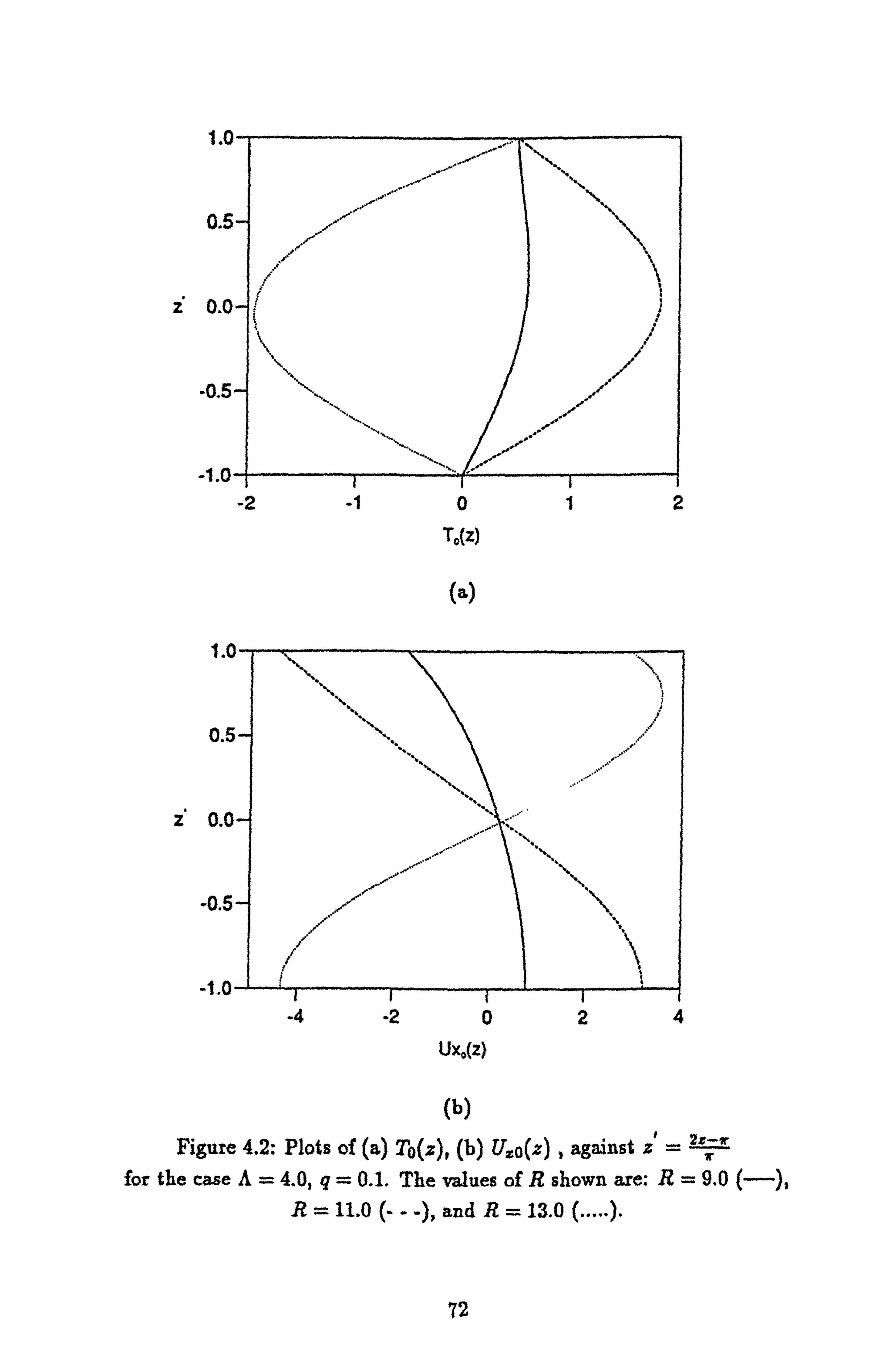
1.1
0.5
Z 0.0
-1.0
-0.5
-2 "1 0 "t 2 T0(z)
(a)
Z
JA
(b)
Figure 4.2: Plots of (a) To(z), (b) U o(z) , against z' =j" for the case A=4.0, q=0.1. The values of R shown are: R=9.0
R= 11.0 (---), and R= 13.0 (..... ).
72
-4 -2 024 Ux (z)
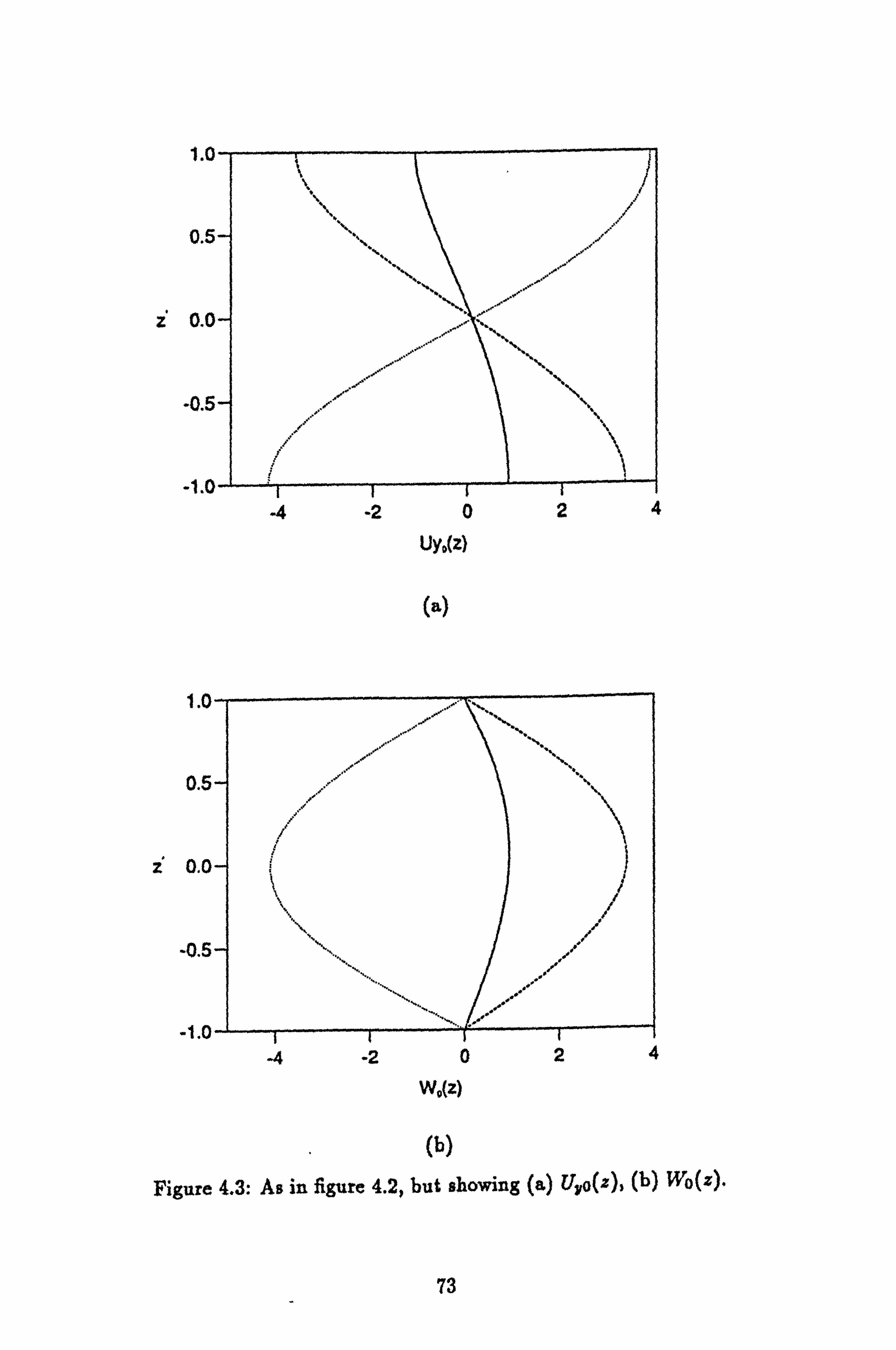
z
UYD(Z)
(a)
Z
W0(z)
(b)
Figure 4.3: As in figure 4.2, but showing (a) TJ, o(z), (b) Wo(z).
73
H4 "2 024
-4 "2 024
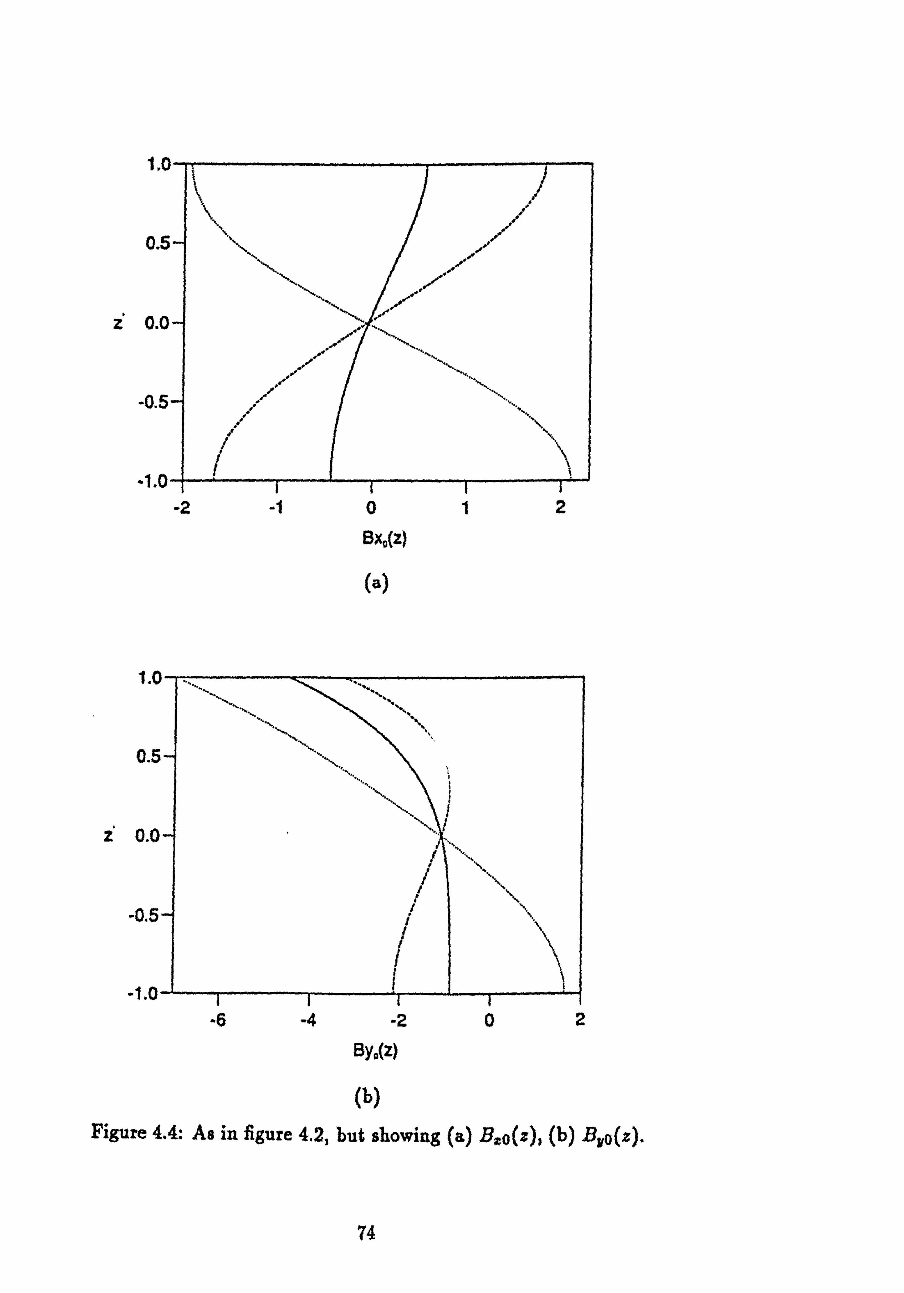
Z
(a)
4n
C
zc
-O
-1
(b)
Figure 4.4: As in figure 4.2, but showing (a) Bzo(z)) (b) B, o(z).
74
-2 -! 012 Bx0(z)
-6 -4 -2 t} 2
8y0(z)

4A
Q
I0
"0
-1
4n
a
Z t?.
-oj
-1. t
-2 -1 012 X0(z)
(b)
Figure 4.5: As in figure 4.2, but showing (a) Bo(z), (b) XO(z).
75
-2 -1 fl 12345 B0(z)
(a)

1.0
0.5
ti z Q. 0 uý..
X
'XX u
yX X. u
X �X
f ýf~
-0.5-
-1.0- -2 -4
Z0(z)
Figure 4.6; As in figure 4.2, but showing Zo(z).
76

2z-ir z=,
ir
(which is chosen so that the layer lies on the interval [-1,1]) for various values of R. The unknowns were found to obey the following conditions
To =Tös
Ux0 =- Uxp,
Uyo = -Uyo,
Wo = Wo,
Bx0 = BxO,
Byo = Byo,
Bo = -Bo,
Xo = -Xä,
Zo = Zo,
(4.21)
so only the relevant real or imaginary part of each unknown is plotted. Only By0 and B0 depend upon the value taken by q, and these are shown for q=0.1. The plots show that the transverse roll forced in the layer by the bumps has
a more complicated z-structure than the free transverse roll that arises in the
77

standard plane layer. This is because the inhomogeneities on To and Bo forbid the
solution from adopting a simple sinusoidal z-structure. The plots also show that
the convection reverses direction above R,, since the solutions change sign once the Rayleigh number exceeds R8.
78
Chapter V
The Stability Of The Basic State
5.1 The Perturbation Equations
Having computed the basic state that arises in a layer with a bumpy top bound-
ary, the next step is to examine the stability of that basic state. This is done by
adding small perturbations to the basic state, and asking whether the perturba- tions grow or decay in time, for given parameter values. If the perturbations grow in time, then the basic state is unstable to the perturbations. But if the pertur- bations decay in time, then the basic state is stable to the perturbations. Of key
importance will be locating the point at which the basic state first loses stability to the perturbations, and what form the onset of instability takes, i. e. does the basic
state lose stability through the exchange of stabilities or through overstability?
Recall, the basic state has the form
X= X(y, z), V=0. (5.1)
Denote the perturbations by Xp and Vp, and set
X= X(y, Z) + SXP(x, y, z, t), (5.2a)
V=0+ SVV(x), (5.2b)
where b«I is a small parameter governing the size of the perturbations. Sub-
stituting (5.2) into the governing equations (2.35), subtracting off the equations satisfied by the basic state, and neglecting all terms of 0(52) or smaller (using the fact that 5 is small), the linear equations governing the perturbations are obtained
79

2aýP+Aý=0, (5.3a) y
2C-A y(V2b, ) - RV2 Op = 0, (5.3b)
w l2ii Jo
(bxbvp + bxpbv)dzdy} = 0, (5.3c) 2Vp - rnqý l21rz
a
q ät -i q(8y)Vý - ýy
- OZbý = Q, (5.3d)
q at
+q (ýy) vp -
äyß - 02sýp
_qýbx d2Vp
_ Q(ab, _ abyl dVp
= 0, (5.3e) dxz ax ay / dx
OOP +
(0 0 v- wp - v28, = 0, (5.31)
°Hbx 219
p- -a äz - Oj' (5.3g)
VHbYP 2
äyez + 19X ' (5.3h)
02wp acp (5.3i) vHuxp
OXOz 5y r
vH2 uyp _a2 yaz + ex. (5.3j)
In a similar manner, the boundary conditions on the perturbations may be obtained from (2.36). They are given by
80
wp=bp yep
=8p=0 on z=0, (5.4a)
wp + mV, sin(my) = bp = Ozp
=O=O on z= 7r. (5.4b)
Now, the basic state takes the form of a transverse roll,
X= Xo(z) exp(imy) + c. c., (5.5)
where
XT(Z) == {To(z) Wo(z) Bo(z) Xo(z) Zo(z)
B o(z) Byo(z) U o(z) Uyo(z)], (5.6)
is the solution of equations (4.6) for the z-structure of the basic state. Recall that (5.5) satisfies Taylor's constraint, and has no geostrophic flow associated with it. The perturbations are assumed to take the form
X, = X-1 (z) exp(ilx - imy + At)+
Xi (z) exp(ilx + imy + At) + c. c., (5.7a)
Vp =U exp(ilx + At) + c. c., (5.7b)
where, for r= ±1,
XT(z) = [TT(z) w, - (Z) B, (Z) x, (Z) Z (z)
Bxr(z) Byr(z) Ur(z) Uyr(z)1, (5.8)
81

represents the z-structure of the perturbations, and U is a constant to be deter-
mined. A is a complex number, defined by
A=9+ iw, (5.9)
where 3 is the growth rate and w is the frequency of the perturbations. (5.7) and (5.8) define a double oblique convection roll (a (+)-roll and a (-)-roll in the notation
of chapter 3), together with the geostrophic flow accelerated by the interaction
of these rolls with the transverse roll forced in the layer by the bumps. In the
standard plane layer model of magnetoconvection, these rolls are the preferred
mode of convection for order one values of A, and have identical linear stability
characteristics. The stability analysis carried out here will ascertain what effect the presence of the transverse roll has upon the stability of these rolls.
Substituting (5.5)and (5.7) into (5.3), the equations for the z-structure of the
perturbations are obtained
2DW_1 - AimX_1 = 0, (5.10a)
2DZ_1 + Aim(D2 - k2)B_1 + Rk2T_1 = 0, (5.10b)
(D2 - k2 - ga)B_1 - imW_1 + gimBoli = 0, (5.10c)
(D2 - k2 - ga)X_1- imZ_, - q(-imXX + 12B* ,0+ lmByo)U = 0, (5.10d)
(D2 - k2 - . \)T_1 + W_1 + imTTU = 0, (5.10e)
k2Bx, _i - i1DB_1 + imX_1 = 0, (5.10f)
k2By, _1 + imDB_1 + ilX_1 = 0, (5.10g)
82

k2Ux, _, - iIDW_1 + imZ_l = 0, (5.10h)
k2Uy, _, + imDW_1 + ilZ_1 = 0, (5.101)
2DW1 + AimX1 = 0, (5.10j)
2DZ1 - Aim(D2 - k2)Bl + Rk2Ti = 0, (5.10k)
(D2 - k2 - qa)Bl + imWi - gimBoU = 0, (5.101)
(D2 - k2 - q. )Xi + imZ1 - q(imXo +l2 Bxp - lmByp)U = 0, (5.10m)
(D2 - k2 - A)Ti + Wi - imToU = 0, (5.10n)
k2Bxi - ilDB1 - imX1 = 0, (5.100)
k2By1 - imDB1 + ilX1 = 0, (5.10p)
k2Uxl - ilDW1 - imZi = 0, (5.10q)
k2Uyl - imDW1 + ilZ1 = 0, (5.10r)
where the coefficient of the perturbation geostrophic flow is given by
83
Zf PZ2grn f (BxQBvl + BxoBy, -i + Bx, -1Byo + BxiBýo)dz. (5.11)
As usual, the following definitions have been made
ä,
k2 = 12 + m2.
The boundary conditions (5.4) are satisfied provided that
W_1 = B_1 = DX_i = T_1 =0 on z=0, (5.12a)
W-1 +i =B_1=DX_1=T_1=0 on z=a, (5.12b)
W1 = B1 = DX1 = T1 =0 on z=0, (5.12c)
Wi-amu=B1=DX1=T1=0 on z=z. (5.12d)
The chief difficulty of solving equations (5.10) and (5.11) is that their coefficients depend upon the basic state X, and X. depends upon the value of the Rayleigh
number R. Thus, for each value of R, the coefficients must first be determined from equations (4.6) before (5.10) and (5.11) can be solved for the perturbations. This means that (5.10) and (5.11) cannot be solved independently of (4.6). Since
the solution of (5.10) and (5.11) must be found numerically, this means that (4.6)
must also be solved numerically, using the same numerical method.
84

5.2 The Numerical Method
Equations (4.6), (5.10) and (5.11) will be solved numerically using spectral methods, which involve approximating the solution of a system of ODE's with an expansion of the form
M E
n=0
called the spectral expansion. M is a positive integer, the constants a, are the
spectral coefficients and
{On n=0,1,2 1, .
is a set of known functions, called basis functions. For this problem, it is convenient to choose
On(z)=PP(z) n=0,1,2,...., (5.13)
where Pn denotes the nth Legendre polynomial, and
zý-2x-7rý (5.14) 7
is chosen so that the interval
0<z<7r,
on which the layer lies, is mapped into the interval
-1<z <1,
on which the Legendre polynomials are defined.
Legendre polynomials are chosen for two main reasons. The first is that they
converge rapidly, so only a few terms of the spectral expansion are needed to give
85

a good approximation to the exact solution. The second reason is that Legendre
polynomials are orthogonal. They satisfy
J-1 P, (z )P'n(z )dz
2n +1' (5.15)
where
1 n=m, Snm =
10 nom,
is the Kronecker delta. This makes evaluating the Taylor integral M much easier, since it can be done analytically using (5.15).
If a function f (z) is expanded in terms of Legendre polynomials as
N f(z)
' j, APn(z »
n=0
where N is an integer, and the coefficients f. are constants, then the derivatives
of f have expansions of the form
N-1 Df =E (D f)nPn(Z ),
n=o
N-2 D2f =E (D2f)nPn(z ),
n=O
where (D f ), l and (DZ f ),, are constants, defined using the recursion relations for Legendre polynomials to be
(D f )n, =- (2n + 1) fp (0 <n<N -1), (5.16a) p=n+l, p+n odd
N
(D2 f )ý, =2 (n + 2) E (p(p + 1) - n(n + 1))fß (0 <n<N- 2). (5.16b)
p=n+2, --
p+n even
86

(See Gottlieb and Orzag 1977). Note that the expansions for Df and D2 f have
N and and N-1 terms respectively, wheras the expansion for f has N+1 terms.
This is caused because the operator D is a lowering operator. That is, it maps the
set of basis functions
{Pn n=0,1, ...., N},
into the set
{Pn : n=0,1,..., N-1}.
The values of f and Df at the boundaries can be obtained using the relations
Pn(±i) = (f1)"ß Pn(±1) = 1n(n
+ 1)(±1)n+1. (5.17)
Now, the problem being solved has inhomogeneous, non-periodic boundary
conditions. Therefore, a spectral method called the Tau method (developed by
Lanczos, 1956) will be used to obtain the solution (see Gottlieb and Orzag, 1977).
To see how the method is applied to a simple equation, see Appendix A.
5.3 The Numerical Solution Of (4.6)
The equations for the z-structure of the basic state are given by (4.6), and
they are to be solved subject to (4.7). These equations were solved previously
using standard methods for linear ODE's, but here, the Tau method will be used. The unknowns are assumed to have the following spectral expansions
87

TO (Z)
Wo(z)
Bo(z)
Xo(z)
Xo(z) = Lo(z) =
Bxo(z)
Byo (z)
U, 0(z)
Uyo(z)
En4 TOnPn(zr
En öi WOn Pn (Z
E2N BOnFn(Z)
Zn ÜZ XOnPn(Z
EN 1=0 ZonPn(Z )
Z. n=o
1 Bxon. PP(z )
, n öi BbonPn(Z )
(5.18)
N' ýn=0 UO pn(z
En 0 UvOnP (z)
where N is an integer and the coefficients of the expansions are complex constants. There are 9N + 18 complex unknowns to be determined using (4.6) and (4.7). The
expansions (5.18) are substituted into (4.6) and (4.7) using (5.16) and (5.17), and
the Tau method is used to derive the following algebraic equations for the spectral
coefficients
4(2n + 1) J\'+2 E Wop + AimXo� =0 (0 <n <_ N),
7r p-n+1 p+n odd
(5.19a)
4(2n -}- 1) N 2(2n .f 1) N+2 z Zop -Aim{ zE
[p(p + 1) - n(n + 1)]Bop -m Bon} p=n+2 p=n+1
p+++ odd p+n even
+Rm2To. =0 (0 < n: 5 N- 1), (5.19b)
88
2(2n + 1) N+2
7r2 E [p(p + 1) - n(n + 1)]BoP - m2Bon + imWo,, =0 (0 <n< N),
p_n+a --
p+n even
(5.19c)
2(2n + 1) N+2
n2 > [p(p + 1) - n(n + 1)]Xop - m2Xpn + imZon =0 (0 <n< N),
p}n even
(5.19d)
2(2n + 1) N+2 Z
7r2 E [p(p+1)-n(n+1)]Top-m Ton-FWon =0 (0 <n< N), (5.19e)
p=n+2 p+n even
m2Bxpn - imXOn =0 (0 <n<N+ 1), (5.19f)
2(2n + 1) N+2 m2Byo, ý - im{ E Bop} =0 (0 <n<N +1), (5.19g)
7r p=n+1
p+n odd
m2Uxon - imZon 0 (0 < n: 5 N), (5.19h)
Z 2(2n -f- 1) N+1 m Uya, ý-im{ E W0P}=0 (0<n<N), (5.19i)
p=n+1 p+n odd
N+1 Z (-1)PW0 = 0, (5.19j) p=O
N+1 wop = 0, (5.19k)
p=0
89

N+2 E (-1)PT0P = 0, (5.191) p=O
N+2 E Top = 2, (5.19m)
P=O
N+2 E (-1)pBop = 0, (5.19n) p=0
N+2 Bop =
2q ,
(5.19o) P=O
N+2 1 E2 (_1)P+lp(p + 1)X0 = 0, (5.19p) p=0
N+21 E ZP(p + 1)Xop = 0. (5.19q)
p=o
(5.19) defines 9N + 18 complex equations in the 9N + 18 complex coefficients of the spectral expansions. In matrix notation, (5.19) takes the form
LoYo = Ro, (5.20)
where Lo is a (9N+18) x (9N+18) complex matrix, RO is a (9N+18) x1 complex vector and YO is the (9N + 18) x1 vector of unknowns defined by
Yö = [Too T01... To, N+2 Woo W01... WO, N+i Boo B01... B0, N+2
X00 X01"""XO, N+2 Z00 Z01"""ZO, N Bx00 B., 01 """Bx0, N+1
Byoo By01... Byo, N+l Uxoo Uxoi... Uxo, N Uyoo Uyo1... UVO, N J. (5.21)
Once suitable values for A, q, m and N have been prescribed, (5.20) can be solved for each value of R using NAG routine F04ADF. This routine uses an LU decom-
position of Lo to solve (5.20) for Yo.
90

5.3.1 Comparison With Chapter 4
To check the validity of the numerical method, the analytic results of Chapter 4 are here reproduced using the Tau method. To do this, the values chosen for the
parameters in Chapter 4, must also be used here.
Attention is restricted to the case
A=4, q=0.1.
The wavenumber m is chosen as in Chapter 4: that is, m2 is chosen to be the
positive root of the cubic
Alms-8m2-8=0.
To choose a value of N, and check for convergence, (5.20) is solved for various values of N at the point R=9.0. At this point, the meansquare heatflux at the bottom boundary is calcualated using the spectral approximation for To(z). Recall that
H= 21DTo(O) 12.
Substituting
To(Z) => To. PP(Z),
n=0
(where the To,, are obtained from Yo) into the definition of H, the following result is obtained
H- 7r
I (-1)n+ln(n + 1)TanI 2
(5.22) n=O
The value of (5.22) for various N at R=9.0 must be compared to the exact value
as calculated in Chapter 4, which is
Hexo, ct = 0.5048671.
91
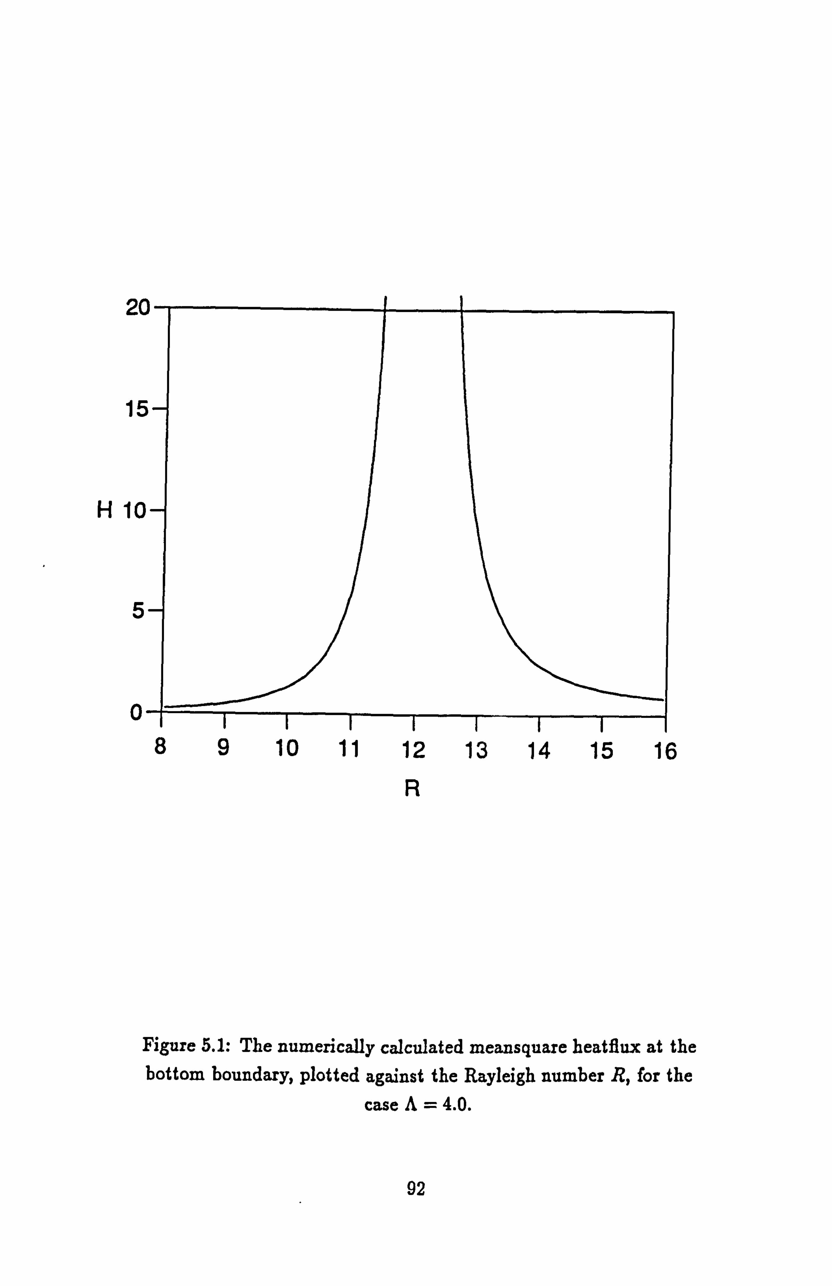
2(
JE
H10
5
0
R
Figure 5.1: The numerically calculated meansquare heatflux at the bottom boundary, plotted against the Rayleigh number R, for the
case A=4.0.
92
89 10 11 12 13 14 15 16

Z
T0(z)
(a)
2
Ux, (z)
(b)
Figure 5.2: Plots of (a) To(z), (b) U,, o(z) , against z' for the
case A=4.0, q=0.1. The value of R shown is R=9.0
93
0.0 0.2 0.4 0.6 0.8 1.0
-2.0 -1.5 -1.0 -0.5 0.0 0.5 1.0

A
Z
(a)
Z
W0(z)
(b)
Figure 5.3: As in figure 5.2, but showing (a) Uyo(z), (b) Wo(z).
94
-2.0 -1.5 -1.0 -0.5 0.0 0.5 1.0 UY0(z)
0.0 0.2 0.4 0.6 0.8 1.0

i
Bx, (z)
(a)
Z
13Y0(z)
(b)
Figure 5.4: As in figure 5.2, but showing (a) Bxo(z), (b) Byo(z).
95
-1.0 -0.5 0.0 0.5 1.0
-5 -4 -3 -2 -1 0

Z
Bo(z)
(a)
Z
(b)
Figure 5.5: As in figure 5.2, but showing (a) Bo(z), (b) Xo(z).
96
012345
-1.0 -0.5 0.0 0.5 1.0
X0(z)

Z(z)
Figure 5.6: As in figure 5.2, but showing Zo(z).
97
-2.0 -1.5 -1.0 -0.5 0.0 0.5 1.0
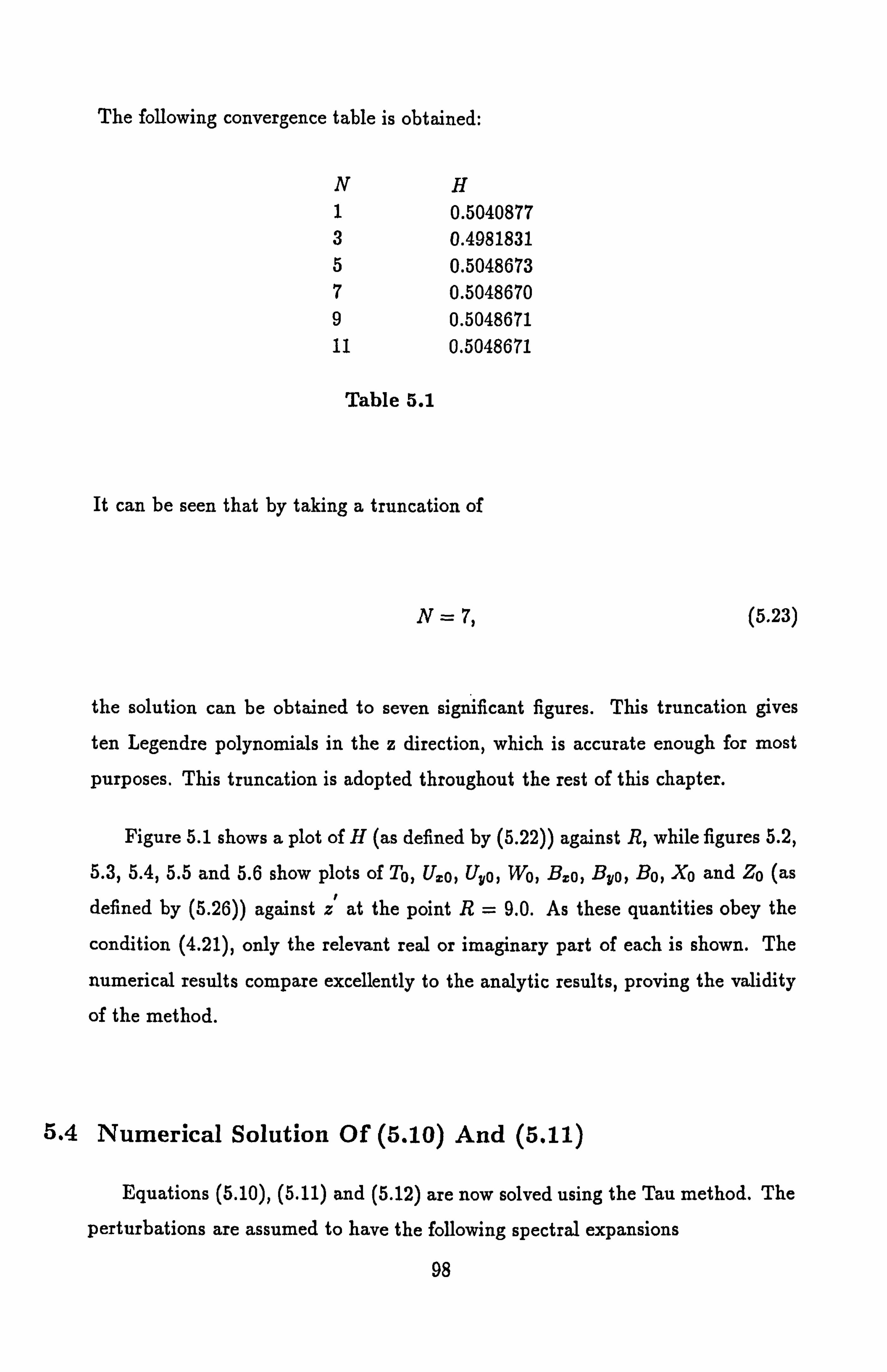
The following convergence table is obtained:
N H 1 0.5040877 3 0.4981831 5 0.5048673 7 0.5048670 9 0.5048671 11 0.5048671
Table 5.1
It can be seen that by taking a truncation of
N=7, (5.23)
the solution can be obtained to seven significant figures. This truncation gives
ten Legendre polynomials in the z direction, which is accurate enough for most
purposes. This truncation is adopted throughout the rest of this chapter.
Figure 5.1 shows a plot of H (as defined by (5.22)) against R, while figures 5.2,
5.3,5.4,5.5 and 5.6 show plots of To, Uxo, Uyo, Wo, Bxo, Byo, Bo, Xo and Zo (as
defined by (5.26)) against z' at the point R=9.0. As these quantities obey the
condition (4.21), only the relevant real or imaginary part of each is shown. The
numerical results compare excellently to the analytic results, proving the validity
of the method.
5.4 Numerical Solution Of (5.10) And (5.11)
Equations (5.10), (5.11) and (5.12) are now solved using the Tau method. The
perturbations are assumed to have the following spectral expansions
98

T, (Z)
Wr(z)
B, (z)
X, (z)
XT(z) = Zr(z) _
Br,. (z)
By,. (z)
Ui, "(z)
Uyr(z)
1: n--+p
TrnPn(z )
ý' p1 WrnPn(Z )
E IV ? BrnPn(xr)
º , nn
o XrnPn(z )
En p ZrnPn(zr
En pý BxrnPn(Zr
cEpl ByrnPn(zr
Nr EN UxrnPn(x
(5.24)
N' Fn_0 UyrnPn(x
where r= ±1. The integer N is the truncation parameter, and is fixed by (5.23).
The coefficients of the spectral expansions are complex constants. There are 2(9N + 18) spectral coefficients to determine from the perturbation equations. Substituting (5.24) and (5.18) into equations (5.10) and the boundary conditions (5.12) using the Tau method, the following linear equations for the spectral coef- ficients of X_1 are obtained
4(2n + 1) N+1 W_1 -- AimX_I� =0 (0 <n< N), (5.25a)
7r p_n+l
p+n odd
4(2n _
1) N 1) N+2 2 Z_p+Aim{2(2n+
7r2 E [p(Pý'1)-n(n-}-1)]B-1p-k B-1n}
p=n+1 p=n+2 p+n odd p+n even
+Rk2T_1n =0 (0 <n<N -1), (5.25b)
99
2(2n + 1) N+2
, r2 > (p(p + 1) - n(n + 1)]B_lp - k2B_ln - imW_In
p=n+2 p+n even
+gimBO*�U = gAB_1� (0 <n< N), (5.25c)
2(2n + 1) N+2 ý2
> [p(p + 1) - n(n + 1)}X_1 -
k2X_1n -
zmZ_in
p-n+2 p-fn even
-q{ - imXX� + l2Bxo� + lmB, *on}U = gaX_1n (0 <n< N), (5.25d)
2(2n -f-1) N+2
72 E [p(p + 1) - n(n + 1)]T_lp - k2T-ln +W -in p_n+2
p+n even
+imTO*�U = AT_1r (0: 5 n< N), (5.25e)
ýzB If 2(2n + 1) N+2 ) x, _lý - . 1{ E B_1p} + imX_1, L =0 (0: 5 n<N+ 1), (5.25f
l p=n+1 p+n odd
(2(2n+1) N+2 k2By, _ln + im > B_1P} + ilX_1ý. =0 (0 <n<N+ 1), (5.25g)
p_n+l p+n odd
2 2(2n -{- 1) N+1 k Ux, _ln - il{ W-lpl + iMZ-In 0 (0 <n <_ N), (5.25h)
r p=ß++1
p+n odd
2 2(2n + 1) N+l k Uý,
_1ý + im{ W_1 } -I- ilZ_1i =0 (0 <n< N), (5.251)
7r Pcn+l
-
p+n odd
100
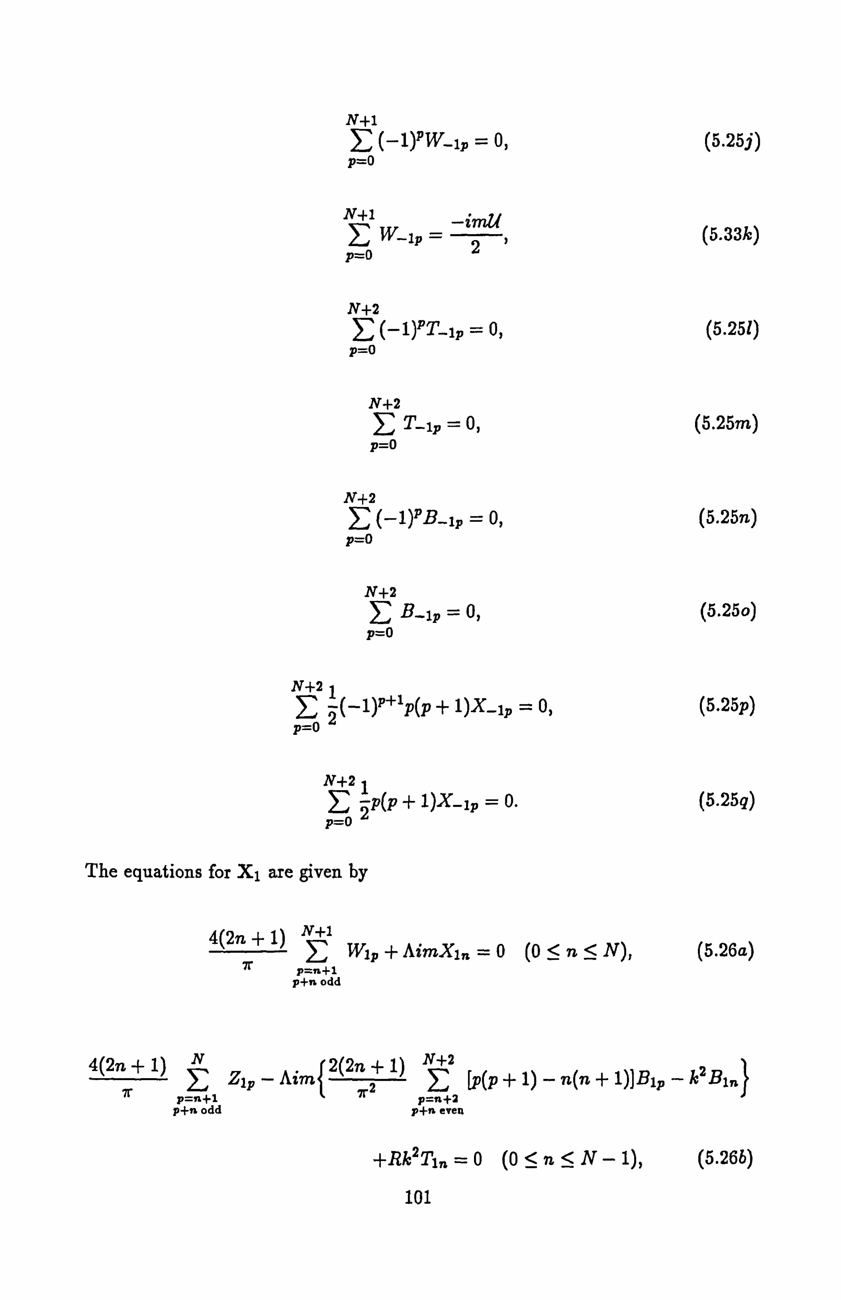
N+1 E (-1)PW_1p = 0, (5.25j) p=O
N+1 EW lp (5.33k)
p, o
N+2 (-1)PT_ip = 0, (5.251)
p=o
N+2 E T_lp = 0, (5.25m) p=0
N+2 S (-1)pB_ip = 0, (5.25n) p=0
N+2 B_lp = 0, (5.25o)
p=0
N+2 1 E2 (_1)P+ip(p + 1)X-lp = 0, (5.25p) p=o
N+21 2 p(p + 1)X_lp = 0. (5.25q)
p=0
The equations for Xl are given by
4(2n + 1) N+l W1p + AimXln =0 (0< n< N), (5.26x)
7r p=n+1
p+n odd
4(2n+ 1) f Zip - Aim{2ý27r2 1ý E [p(p + 1) - n(n + 1))Blp - k2Bln}
p=n+1 p=a+2 p+n odd p+n even
+Rk2T1� =0 (0 <n<N- 1), (5.26b)
101

2(2n + 1) N+2
72 E [p(p + 1) - n(n + 1)]Blp - k2B1, + imWi,
P=n+2 p+n even
-gimBonU = q)Bin (0: 5 n< N), (5.26c)
2(2n + 1) N+2 ý, 2
7.2
E [p(P + 1) - n(n 1)]X1 -k Xln + imZln
p=nß-2 p}n even
-q{imXpn + 12Bxp, 4 - lmByo }U = gAXln (0: 5 n< N), (5.26d)
2(2n+1) E [p(p+1)-n(n+1)]Tlp-k2
7r2 Tin+W1n
p-nß-2 p1-n even
-imTo�U = \T1, ß (0 <n< N), (5.26e)
k2B 2(2n +, 1) N+2 x, ln -ill > Blp} - imXl,, =0 (0 <n<N+ 1), (5.26f )
T p_n+l
p+n odd
k2By, in. - im 2(2n + 1) N+2
B1 }+ ilXln =0 (0 <n <_ N+ 1), (5.26g) p=n}1
p+n odd
k2Ux 2(2n + 1) Iv+l , iý - il{ E Wip} - im2 =0 (0 <n< N), (5.26h)
p=n+1 -
p+n odd
k2Uy, ln - im 2(2n }1) N+1
> wip} + ilZ1 =0 (0 _< n <_ N), (5.261)
p=n+1 p+n odd
102

N+1 E (-1)pwlp = 0, (5.26j)
p=o
N+1 imu Y' Wlp = (5.26k) P=O
N+2 r, (-1)PTip = 0, (5.261)
p=o
N+2 r, Tlp = 0, (5.26m)
p=O
N+2 E (-l)"Blp = 0, (5.26n) P=O
N+2 Blp = 0, (5.26o)
p=o
N+2 1 Z 2(_1)n+1p(p+ 1)X11, = 0, (5.26p) P=o
N+21 E
2p(P + 1)Xlp = 0. (5.26q)
p=0
Equations (5.25) and (5.26) define 2(9N + 18) complex, linear algebraic equations in the 2(9N + 18) complex spectral coefficients. It now just remains to evaluate equation (5.11) for the coefficient U of the geostrophic flow using the Tau method. Using the orthogonality condition (5.15) this equation becomes
I'ilAg N+i 1 2 2n +1
{B; OBY1n + BonBV, -ln + Bz, -1nByon + Bx1nBYOn} = 0.
n=O (5.27)
Defining U as an unknown, and combining (5.25), (5.26) and (5.27), a system of 18N + 37 complex, linear algebraic equations in 18N + 37 complex unknowns is
103

obtained. In matrix notation, this system takes the form of a generalised eigenvalue problem,
LpYp = ARYp, (5.28)
where Lp and R7, are complex matrices of size (18N + 37) x (18N + 37) and Yp is
the (18N + 37) x1 vector of unknowns. If Yp is partitioned as follows,
Yp YpT YpB
where Yp ' is a (6N + 6) x1 vector of unknowns defined by
YpT = [T_1OT_ll... T_INB_1OB_11... B_1NX_10X_11... X_1N
Tio Tll... TIN Blo Bil ... BiN Xio Xii ... XlN 11 (5.29)
and YOB is a (12N+31) x1 vector containing the remaining unknowns, then (5.28)
takes the form
L11 L12 YPT =A
Iert+e 0 YPT [L21 L22
[ypBI 100 YPB '
where L11 is a matrix of size (6N + 6) x (6N + 6), L12 is a matrix of size (6N +
6) x (12N + 31), L21 is a matrix of size (12N + 31) x (6N + 6) and L22 is a matrix
of size (12N + 31) x (12N + 31). I6N+6 denotes the (6N + 6) x (6N + 6) identity
matrix. Therefore, the equations
LilypT + L12YpB = AypTs
L2IYpT + L22YpB = 0,
are obtained. These can be rearranged to give the matrix equations
104
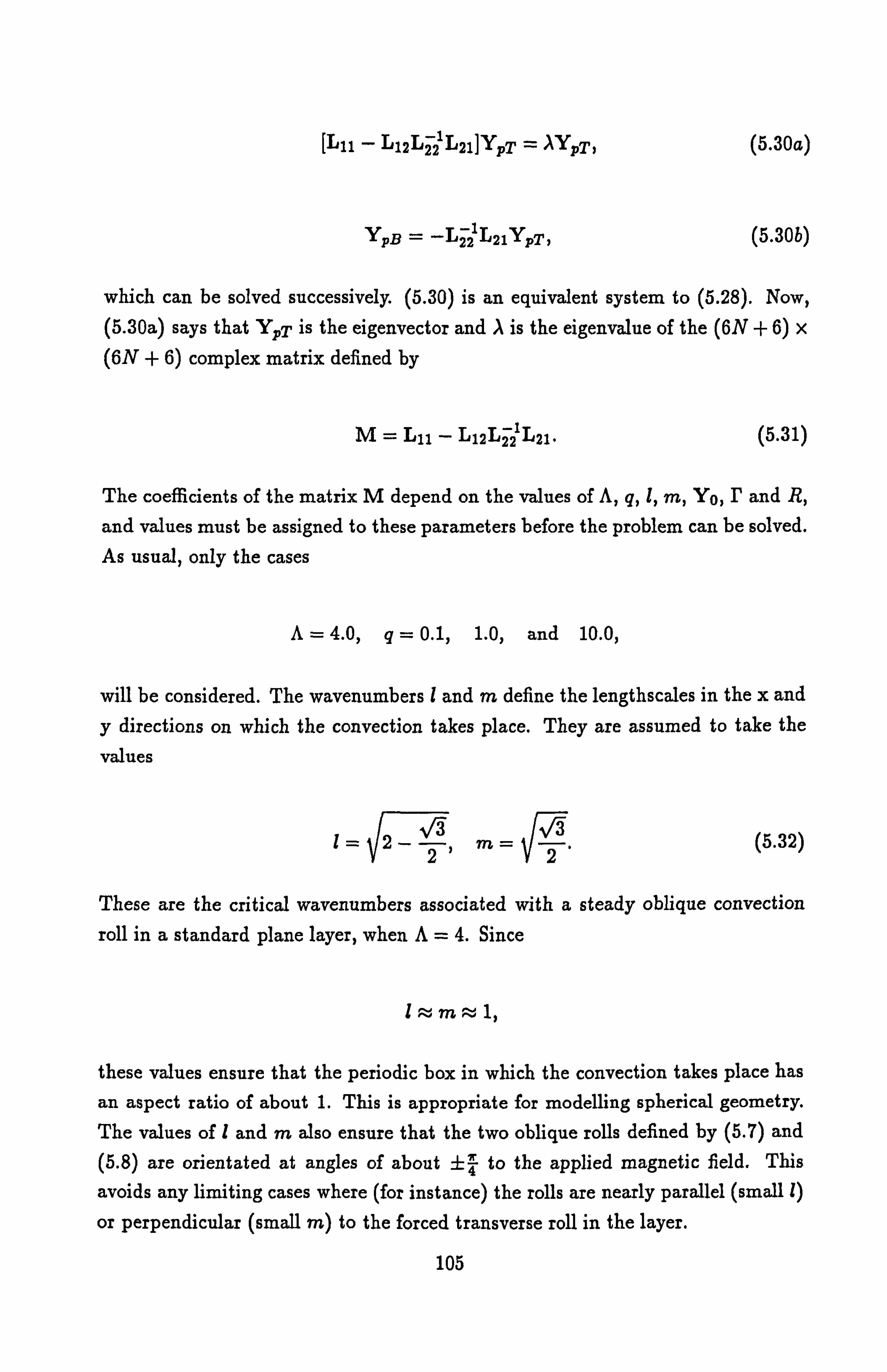
[Lii - L12L22 lL2lIYpT = AYpTi (5.30a)
YpB = -L22iL21YpT, (5.30b)
which can be solved successively. (5.30) is an equivalent system to (5.28). Now, (5.30a) says that YpT is the eigenvector and A is the eigenvalue of the (6N + 6) x (6N + 6) complex matrix defined by
M= Lll - L12Liz L21. (5.31)
The coefficients of the matrix M depend on the values of A, q, 1, m, Yo, P and R,
and values must be assigned to these parameters before the problem can be solved. As usual, only the cases
A=4.0, q=0.1,1.0, and 10.0,
will be considered. The wavenumbers l and m define the lengthscales in the x and
y directions on which the convection takes place. They are assumed to take the
values
l= 2- 2
M- 2
(5.32)
These are the critical wavenumbers associated with a steady oblique convection roll in a standard plane layer, when A=4. Since
Istlm;:: ýl 1,
these values ensure that the periodic box in which the convection takes place has
an aspect ratio of about 1. This is appropriate for modelling spherical geometry. The values of d and m also ensure that the two oblique rolls defined by (5.7) and (5.8) are orientated at angles of about ±1 to the applied magnetic field. This
avoids any limiting cases where (for instance) the rolls are nearly parallel (small 1)
or perpendicular (small m) to the forced transverse roll in the layer.
105

Finally, ranges of values of R and r are chosen. For each required value of R
and F, equations (5.20) are solved for YO using the prescribed parameter values. Then, the matrix M is set up, and NAG routine F02AKF is employed to find
the 6N +6 eigenvalues A and eigenvectors YPTJ of M. This routine works by first finding a transformation that converts M to Hessenberg form, Mg. Then,
an LR decomposition of Mg is used to find the eigenvalues and eigenvectors of Mg. These are then mapped to the eigenvalues and eigenvectors of M using the inverse transformation. A simple matrix multiplication routine then gives YpB3
from YpTJ. In this way, the 6N +6 eigenvalues A, and eigenvectors Ypj of (5.28)
are obtained for each required value of R and F.
5.4.1 The Stability Criteria
The following definitions are made
si = RE(aj), j=1,2, ..., (6N + 6), (5.33a)
wi = IM(A ), j=1,2, ..., (6N + 6). (5.33b)
Each eigenvector Ypj gives a possible z-structure for the perturbations. Each sj
represents the growth rate, and wi the frequency, of the perturbations whose z-
structures are given by the eigenvector Yp,. The stability characteristics of these
perturbations are found by looking at the sj and the wj.
Now, the sj can be ordered so that
si>s2>83>..... >9(6N+s)" (5.34)
With A, q, Z and m fixed, the growth rates only depend upon the values taken by
r and R. Hence
9J = sj(r, R) Vj. (5.35)
It transpires that the stability of the basic state depends upon the sign of al, the largest growth rate. To see this, note that if
106
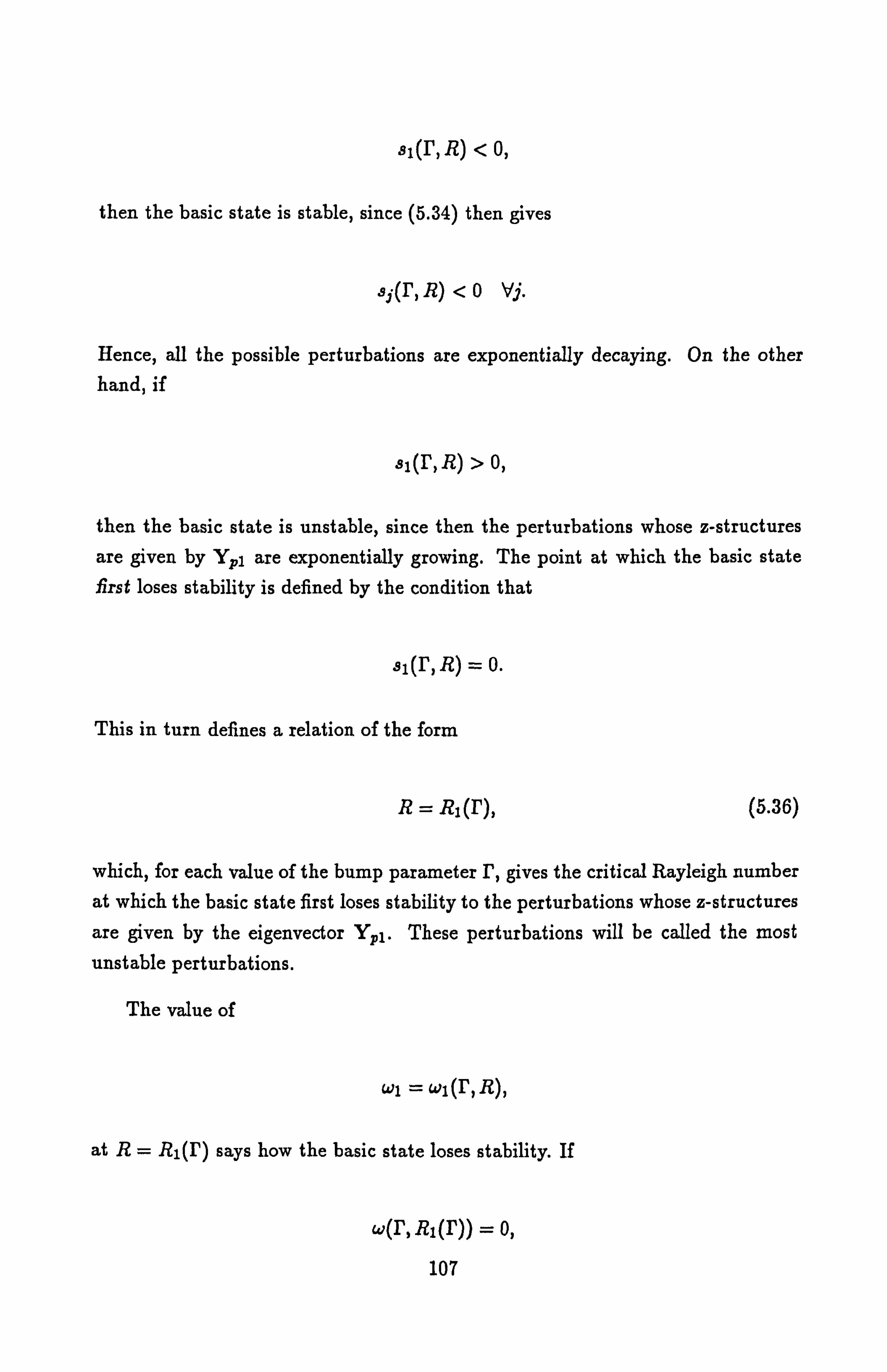
sl(r, R) < o,
then the basic state is stable, since (5.34) then gives
9; (r, R) <0 Vj.
Hence, all the possible perturbations are exponentially decaying. On the other hand, if
31(r, R)>0,
then the basic state is unstable, since then the perturbations whose z-structures are given by Yi, 1 are exponentially growing. The point at which the basic state first loses stability is defined by the condition that
31(r, R) = o.
This in turn defines a relation of the form
R= RI (r), (5.36)
which, for each value of the bump parameter r, gives the critical Rayleigh number at which the basic state first loses stability to the perturbations whose z-structures are given by the eigenvector Y, 1. These perturbations will be called the most unstable perturbations.
The value of
w, = wl (r, R),
at R= R1(r) says how the basic state loses stability. If
w(r, Ri(r)) = 0,
107

then the basic state loses stability through the exchange of stabilities. However, if
w(r, Ri(r)) 0,
the the mechanism is overstability, and the frequency of the perturbations at crit- icality is given by wi (P, RI (r)).
The stability criteria for each of the other possible perturbations that arise can be derived by analogy with those for the most unstable perturbations.
5.5 Results
In this section, the stability characteristics of the most unstable perturbations, for the chosen parameter values, are described. These characteristics define where
and how the basic state first loses stability for the given parameter values. For
comparison, the stability characteristics of the perturbations whose z-structures
are given by Y, 2 are also described. These perturbations have the second largest
growth rate, s2, and will be called the second most unstable perturbations.
5.5.1 The Most Unstable Perturbations
This is the preferred mode of instability for the basic state. It consists of a double oblique roll (i. e. a linear combination of a (+)-roll and a (-)-roll in the
notation of chapter 3). These two rolls align themselves with the transverse roll forced by the bumps in such a way that Taylors constraint is satisfied at O(5), so the solution satisfies
2a m
Jm (axabvp ' bxpbýo)dady= 0. äx 21r2 of1
(5.37)
Hence, the perturbations do not accelerate a geostrophic flow when they interact
with the basic state, so V. = 0. A consequence of this surprising result is that the
stability characteristics of these perturbations are independent of the values taken by r and q. The critical Rayleigh numbers at which the basic state loses stability to these perturbations, which are defined by
108

R= R1(r), (5.38)
turn out to be the same, no matter what value of P is chosen. In fact, the basic
state loses stability to these perturbations once R exceeds
Rl = 10.39230485 = 6V,
irrespective of r. A graph of (5.38) against r is a straight line in the (T, q) plane (this is shown in figure 5.7). It turns out that the frequency associated with these
perturbations satisfies
wl(r, Ri(r)) = o.
Again, this is irrespective of the value of F. Hence, the basic state loses stability to these perturbations through the exchange of stabilities mechanism (at least, for
the parameter values chosen). Figure 5.8 shows a plot of sl and wl against R.
In figures 5.9,5.10,5.11,5.12 and 5.13 the z-structure of the perturbations are plotted against z', when R= R1. These figures show that the unknowns
adopt simple sinusoidal profiles at criticality. The solutions can adopt such simple z-structures since with no geostrophic flow forced by the interaction of the per- turbations with the basic state, there is no forcing on the perturbations, and the boundary conditions on the perturbations become homogeneous. Simple, homoge-
neous boundary conditions can easily be accomodated by sinusoidal profiles. Note
that the unknowns obey the conditions
Tr = -Tr',
Uxr = UxOr
Uyr = Uyr
109
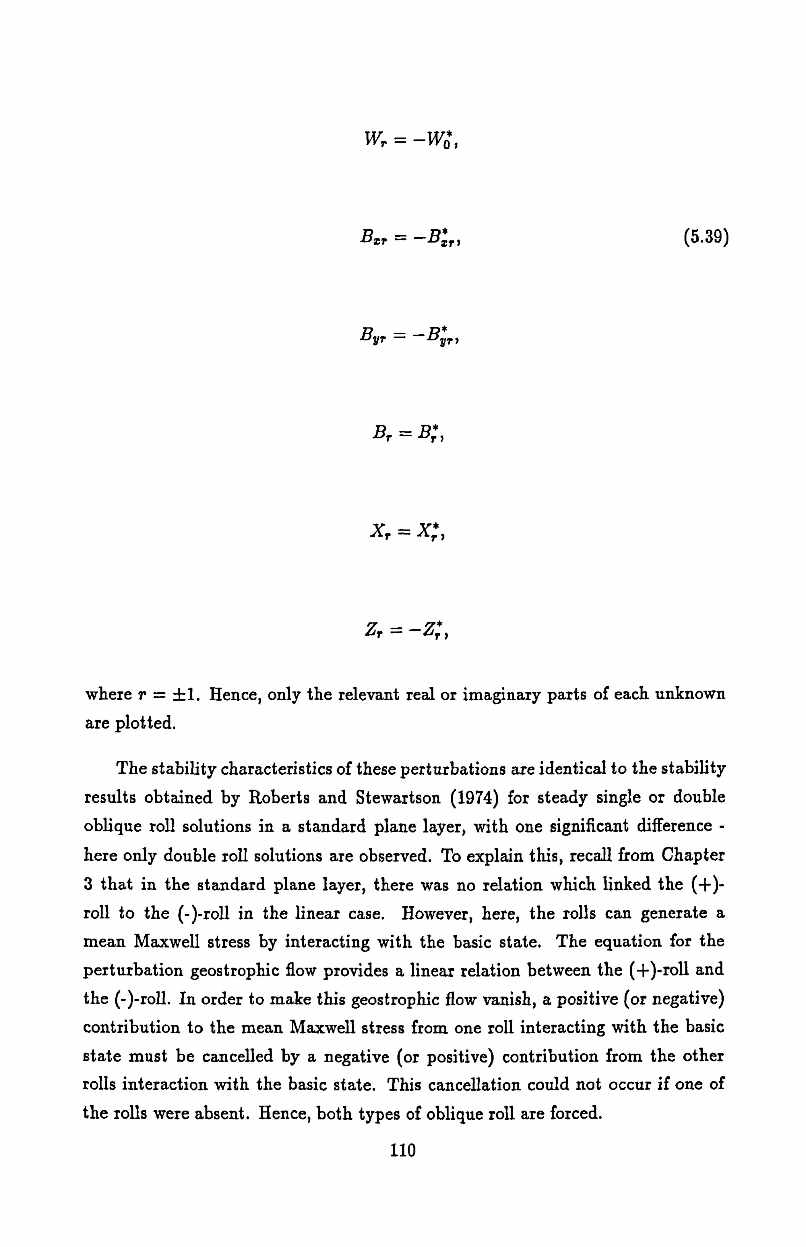
s Wr = -Wo ý
Bx, _ -Bx, , (5.39)
B7/T - -BlJTf
Br = Br I
X* ° Xr,
ZT=-z;,
where r= ±1. Hence, only the relevant real or imaginary parts of each unknown
are plotted.
The stability characteristics of these perturbations are identical to the stability
results obtained by Roberts and Stewartson (1974) for steady single or double
oblique roll solutions in a standard plane layer, with one significant difference - here only double roll solutions are observed. To explain this, recall from Chapter
3 that in the standard plane layer, there was no relation which linked the (-)-
roll to the (-)-roll in the linear case. However, here, the rolls can generate a
mean Maxwell stress by interacting with the basic state. The equation for the
perturbation geostrophic flow provides a linear relation between the (+)-roll and the (-)-roll. In order to make this geostrophic flow vanish, a positive (or negative)
contribution to the mean Maxwell stress from one roll interacting with the basic
state must be cancelled by a negative (or positive) contribution from the other rolls interaction with the basic state. This cancellation could not occur if one of the rolls were absent. Hence, both types of oblique roll are forced.
110

5.5.2 The Second Most Unstable Perturbations
When the z-structures of the perturbations are given by YY2, their stability characteristics change quite drastically. Again, the perturbations consist of a dou- ble oblique roll solution. Now, however, these rolls interact with the transverse
roll forced by the bumps to accelerate a geostrophic flow of the form
V. =U exp(ilx) + C. C.,
in the layer. Consequently, the stability characteristics of these perturbations are no longer independent of r or q.
The critical Rayleigh numbers at which the basic state loses stability to these
perturbations are defined by a relation of the form
32(r, R) = o,
where s2 is the second largest growth rate. This relation yields
R=R2(r), (5.40)
which for each value of r gives the critical Rayleigh number at which the basic
state loses stability to these perturbations. (5.40) defines curves in the (I', R)
plane. These curves are plotted for the three values of q chosen in figures 5.14, 5.15 and 5.16. It transpires that
w2(r, R2(r)) - o,
for each value of r (where w2 is the frequency associated with these perturbations). Hence, the basic state loses stability to these perturbations through the exchange of stabilities (again, this is only for the parameter values examined).
The s-shape of these marginal stability curves may be explained by examining figure 5.17, which shows a plot of s2 and w2 against R, for the cases r=0.05, r=0.2, P=0.35 when q=0.1. The e2 curve consists of two branches: the first branch exists for
ill

R,
10
5
0
r
Figure 5.7: A Plot of R1(r) against r.
112
0.0 0.05 0.1 0.15 0.2 0.25
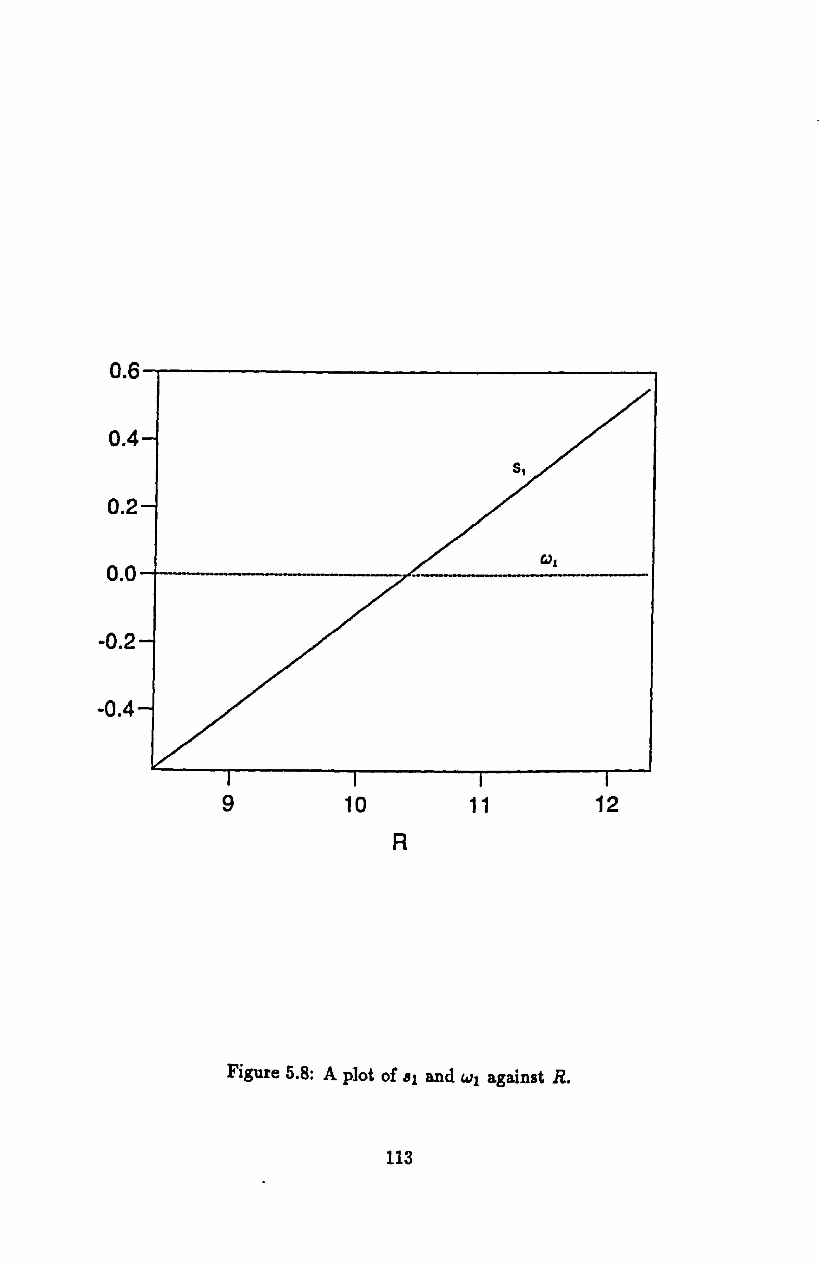
0.6
0.4 SI
0.2
0.0
-0.2
-0.4
tit
9 10 11 12
R
Figure 5.8: A plot of al and wl against R.
113

1.0
0.5
2 0.0
-1.0
-0.5
0.0 0.1 0.2 0.3 0.4
(a)
Z
(b)
Figure 5.9: Plots of (a) T_1(z) (-), T1(z) (- - -) (b) Ux, _1(z) (--), Ux, 1(z) (' ' -)
against z' at the point R= R1.
114
-1.5 -1.0 -0.5 0.0 0.5 1.0 1.5

Z
(a)
1
0
Z0
-a
.1
(b)
Figure 5.10: As in figure 5.9, but showing (a) Uy, _i(z) (-), Uyi(z) (- - -)s
(b) W i(z) (--)' W1(z) (- - -).
115
-1.0 -0.5 0.0 0.5 1.0
0.0 0.2 0.4 0.6 0.8 1.0 1.2

Z
(a)
2
(b)
Figure 5.11: As in figure 5.9, but showing (a) Bx, _1(z) (-), Bi(z) (- - -),
(b) Bv, -i(z)
(-), Byi(z) (- - -).
116
-0.4 -0.2 0.0 0.2 0.4
-02 -0.1 0.0 0.1 0.2

Z
(a)
Z
(b)
Figure 5.12: As in figure 5.9, but showing (a) B_i(z) (-), Bi(z)
(b) X-i(z) (_"), Xi(z) (- - -).
117
-0.4 -0.3 -0.2 -0.1 0.0
-0.5 0.0 0.5

Z
-o
-1
Figure 5.13: As in figure 5.9, but showing Z_1(z) (-), Zi(z) (- - ).
118
-2 -1 012

R<R,,
(where R, is the value of the Rayleigh number at which the basic state is singular, as defined in Chapter 4) while the second branch exists for
R>R,.
The points where the 82 curve crosses the R axis define the critical Rayleigh num- bers for these perturbations. Multiple critical Rayleigh numbers arise because 82 satisfies
S2 -- -oo as R-> Rä .
This says that the basic state is stable to these perturbations in the region of it's
singularity. However, if the 82 curve crosses the R axis below R, (i. e. on the first branch), then it must do so again to satisfy this condition. Since the second branch
always crosses the R axis, multiple critical Rayleigh numbers are obtained for those
values of r at which the first branch can cross the R axis. As always, however,
it is the perturbations with the smallest associated critical Rayleigh numbers that
will be preferred at a given value of r.
Note also from figure 5.14,5.15 and 5.16 that
R2(r)-moo as r -->oo,
so increasing the bumpsize parameter makes the basic state more stable to these
perturbations. This may be traced to the fact that larger values of r increase the
strength of the geostrophic flow. This increases the shear generated by VP, and since shear suppresses convection (Fearn and Proctor 1983b; Fearn 1989) this leads to an increase in the critical Rayleigh number.
In figures 5.18,5.19,5.20,5.21 and 5.22 the z-structure of these perturbations are plotted against z', when r=0.1, R= R2(0.1) and q=1.0. These perturba- tions also obey (5.39), so only the relevant real or imaginary part of each is plotted. Figure 5.23 shows the geostrophic flow profile set up by the interaction of the
119

14
13
R212
11
10
r
Figure 5.14: A plot of R2(r) against r in the case q=0.1.
120
0.0 0.05 0.1 0.15 0.2 0.25

14
13
R212
11
10
r
Figure 5.15: A plot of R2(r) against r in the case q=1.0.
121
0.0 0.05 0.1 0.15 0.2 0.25

14
13
R212
11
10
*10-3
r
Figure 5.16: A plot of R2(r) against r in the case q= 10.0.
122
01234

1.0
0.5
0.0
-0.5
Figure 5.17: A plot of s2 (--) and w2 (- - -) against R for the cases r, = 0.05,0.2,0.35 when q=0.1.
123
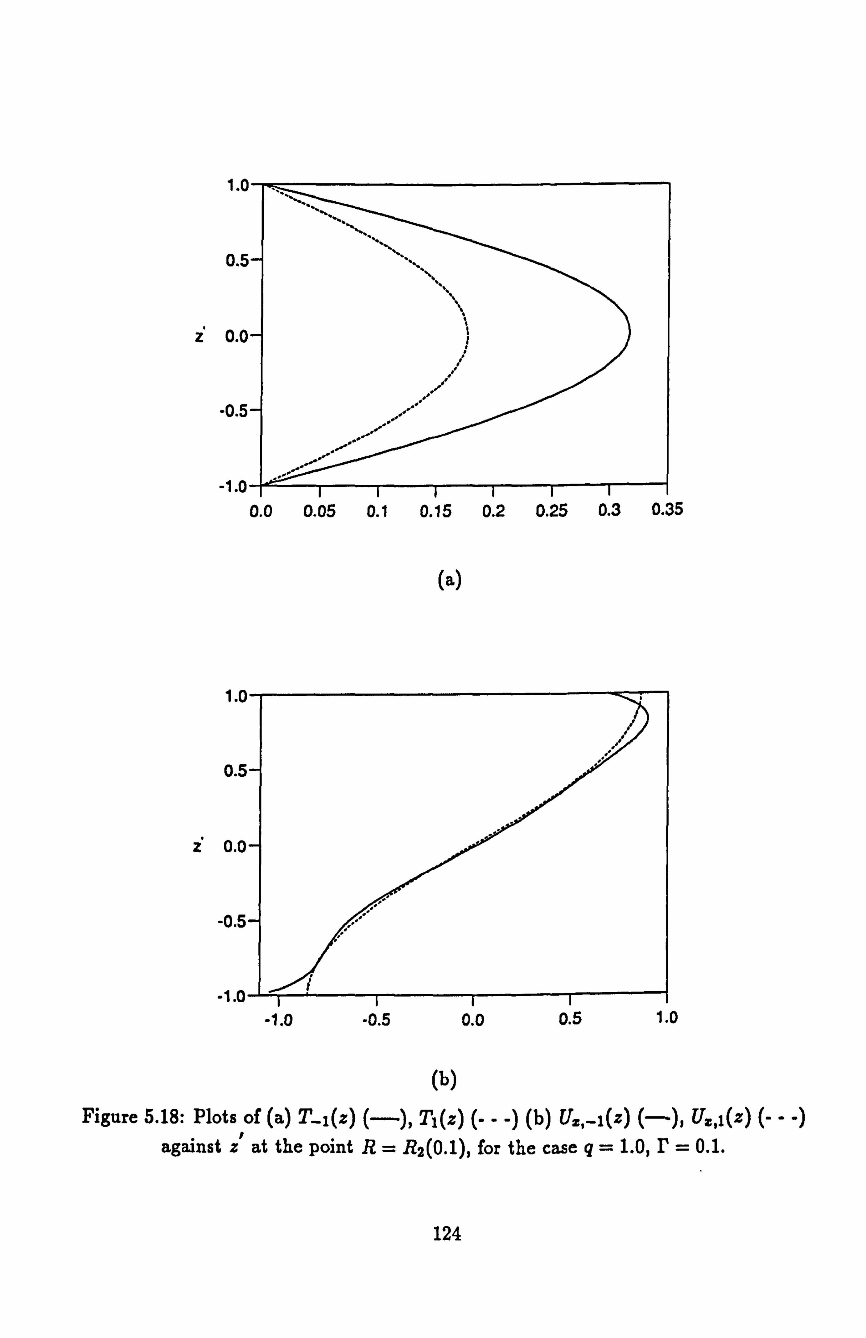
Z
(a)
z
(b)
Figure 5.18: Plots of (a) T_1(z) (--), Ti(z) (- - -) (b) Ux, _1(z)
(--), UU, l(z) (- - -) against z' at the point R= R2(0.1), for the case q=1.0, r=0.1.
124
0.0 0.05 0.1 0.15 0.2 0.25 0.3 0.35
-1.0 -0.5 0.0 0.5 1.0

2
(a)
1
0
ZG
-0
-1
(b)
Figure 5.19: As in figure 5.18, but showing (a) Uy, _i(z) (-), Uyl(z) (- - -),
(b) W1 (z) (--), Wi(z) (- - -).
125
-1 012
0.0 0.2 0.4 0.6 0.8 1.0 1.2

2
(a)
1.0
o.:
z 0.0
-1.0
-0.5
-0.4 "-0.2 0.0 0.2 0.4
(b)
Figure 5.20: As in figure 5.18, but showing (a) Bz, -i(z) (-), Bxl(x) (- - -),
(b) Bv, -i(z)
(--), Bvl(z) (- - -).
126
-0.3 -0.2 -0.1 0.0 0.1 0.2 0.3

1.
o.
Z 0.
-o
.1
.3 -0.2 -0.1 0.0
(a)
"rr,.
,5Jf;
f"
. 0.0
1
0
z0
-a
-1
(b)
Figure 5.21: As in figure 5.18, but showing (a) B_1(z) (-), Bl(z) (- - -), (b) X-1(z) (--)' Xl(z) (- - -).
127
-0.5 0.0 0.5

Z
Figure 5.22: As in figure 5.18, but showing Z_I(z) (-), Zi(z) (- - -).
128
-3 -2 -1 0123

4
2
xO
_2
-4
V(x)
Figure 5.23: V(x) against x at R= R2(0.1), r=0.1, q=0.1.
129
-0.2 -0.1 0.0 0.1 0.2

perturbations with the basic state. The presence of a non-zero geostrophic flow
means that the perturbations are inhomogeneously forced by the interaction of this flow with the bumps. These inhomogeneities forbid the perturbations from
adopting simple sinusoidal profiles. The z-structures of these perturbations are more complicated than those of the most unstable perturbations, and this explains why these perturbations have a larger critical Rayleigh number associated with them: it takes more energy to excite a complicated z-structure.
5.5.3 The Behaviour As IF -+ 0
Examination of figures 5.14,5.15 and 5.16 reveals that
R2 -º 6v-f3- = R1 as P --> 0.
This occurs because in this limit, the effects of the geostrophic flow upon the second
most unstable perturbations vanish, since
Vý-ý0 as r--+0.
The reduced effect of V. allows the second most unstable perturbations to adopt
simpler z structures, while the reduced shear allows the convection to occur more
easily, leading to a smaller critical Rayleigh number for these perturbations.
For small, finite r, the two sets of perturbations remain distinct, the most
unstable perturbations being the preferred mode of instability. However, when r
becomes zero, do the two types of perturbations coalesce to form a single, unique
mode of instability? Or do they remain two distinct modes of instability, having a
common critical Rayleigh number (as in the case of single and double oblique roll solutions in the standard plane layer).
It transpires that that this question does not arise at all for this problem, since r must remain finite and non-zero to have a solution of this problem. To see this,
recall (from the definition of r) that
r=0= =0, 130
and so zero r corresponds to the no bump case. But, the convective motions described here are all topographically forced, i. e. they are forced by the bumps. So, as r --+ 0, this forcing vanishes, and the convective motions evaporate. In the
no bump limit, the solution (2.24) that is being examined collapses back onto the hydrostatic conduction solution. Therefore, the solutions considered here are only valid for non-zero values of r.
5.6 A Check On The Numerics
To check the linear stability results quoted in the previous section, the pertur- bation equations were solved in the limit of small but finite r, i. e. for those values of r which satisfy
0<r<1. (5.41)
The exact details of the calculation are given in Appendix B, but the main results
will be discussed here.
The equations yield an analytic solution for the perturbations which takes the
form of a double oblique roll,
Xp = {alX_1RS(z)} exp(ilx -- imy + iwcot)+
{-a2X 1RS(z)} exp(ilx + imy + iwcot) + c. c., (5.42)
where the complex constants al and a2 are defined by (B. 25) and X±1RS(x) are the Roberts and Stewartson (+) and (-) oblique roll solutions defined in chapter 3. These perturbations interact with the basic state in such a way that no geostrophic flow is accelerated, so
Vp=0. (5.43)
The fact that no geostrophic flow is accelerated means that this solution is inde-
pendent of r. That is, the solution is valid for all non zero values of r, not just for those values which satisfy (5.41).
131
The values of R, and we at which this solution exists are defined by (B. 19) and (B. 20), namely
wcp = 0,
R, o = 4(1 + k2)2
+ Am2(1 + k2)
Am2k2 k2
for the exchange of stabilities case, and
2 (4 -1)A2m4(1 + k2) - 4(4 + 1)2(1- k2)2 wco 4g2(1 + q)2
_ 2j 4(1 + q)(1 + k2)2 Am2(1 + k2)
Re0 ql Am2k2 + k2(1 + q)
}.
for the overstable case. These stability results are identical to those obtained by Roberts and Stewartson (1974), and quoted in chapter 3, for the stability of the hydrostatic conduction solution to perturbation by oblique convection rolls in the
standard plane layer. Hence, all the stability results of chapter 3 are applicable here for the solution (5.42) and (5.43).
Hence, quoting from chapter 3, the basic state (i. e. the transverse roll forced by the bumps) loses stability to the perturbations (5.42) through the exchange of stabilites once R exceeds
Re=6V,
the critical wavenumbers being given by
2 2V3 2 2/ -A, is=2- -T-, MC =
It loses stability to (5.42) through overstability once R exceeds
12i
4
132

the frequency of the perturbations being given by
we _ 9(gqZ 2)
and the critical wavenumbers for this case being
12 =2- 2ý (1 + 4), me 2= 2A
(1 + 4).
The exchange of stabilities is preferred in the region
q<2, A>v and q>2, vr3- <A<VY(1+q),
while overstability is preferred in the region
q>2, A> /(1 + q).
These oblique perturbations do not exist in the region
A<NF3,
This is because oblique convection rolls are not supported by weak magnetic fields. As A is decreased towards V3-, the axis of the oblique rolls become parallel to that
of the transverse roll forced by the bumps, and hence, do not perturb it. For this
reason, the basic state is stable to perturbation by oblique rolls for weak magnetic fields. These stability results are shown in figure 5.24.
These results can be used to check the results obtained numerically in the
previous section. To do this, recall that the most unstable perturbations deter-
mined numerically (i. e. the perturbations whose z-structures were given by Y 1) have the same characteristics as the solution (5.42) determined in Appendix B. They have simple sinusoidal z-structures, obey Taylor's constraint (i. e. accelerate no geostrophic flow through interaction with the basic state) and have the same stability characteristics as the Roberts and Stewartson oblique roll solutions in the
standard plane layer. Therefore, (5.42) is the analytic form of the most unstable
133

10
8
6
A
4
2
0
q
Figure 5.24: The regions of the (q, A) plane where the basic state loses stability to the perturbations through overstability (region I)
or through the exchange of stabilities (region II). The perturbations do not exist in region III, so the basic state is stable there.
134
02468 10

perturbations found previously. To check the numerics, therfore, the numerical results obtained previously will be compared to these analytic results at the point
A=4.
As the stability results indicate that the exchange of stabilities is valid at this value of A, the critical wavenumbers are given by
1Z=2- 2,
m2= 2
(5.44)
This justifies a postiori the choice (5.32) made for l and m, since it has been shown that these are in fact the critical values for this stability problem. At this value of A, al and a2 take the values
al = ql{(4l - m)1 - (Ofm + 1)1,1 , (5.45a)
a2 = ql {(Vl
+ m)12 - (l - 'vr3m)ll (5.45b)
where the integrals Il and 12 are defined by (B. 26). Figure 5.25 shows a plot of Ia1J2 and 1a212 against q for A=4.
Now, from the definitions of X±1RS,
T_1 = alsin(z), Tl = -a2 sin(z).
Using this, it can be shown that
ja112 _
fö T_lT*ldz (5.46) Tanz fö TiTidz
The quantity on the left hand side of (5.46) is plotted against q in figure 5.26(a).
The spectral approximations to TT1 are given by
135

300
200
100
0
q
Figure 5.25: A plot of Jai12 (--) and Ja212 (- - -) against
q for the case A=4.
136
02468 10

(a)
(b)
Figure 5.26: These graphs show plots of the ratio T 1T= ldz against q,
o TIT; dz
using (a) the analytic results, (b) the numerical results.
137
0123456789 10
q
0123456789 10
q

N+2 TTY =E T±iPn(x ),
n=0
where N=7, P,, is the nth Legendre polynomial and z' is defined by (5.14). The constants T±1, ti are obtained from the eigenvector Yi, 1, obtained numerically. Using the orthogonality condition that holds for Legendre polynomials, it can be
shown that
FN+2 T' in 2 Jo T_iT*ldx +ý-o zn+l (5.47) N+a Tlm' - fo TIT , *dz
'M=O 2m+i
The quantity on the left hand side of (5.47) is plotted against q in figure 5.26(b).
The results (5.46) and (5.47) indicate that the two curves should be identical,
and this is borne out by the graphs in figure 5.26. This confirms that (5.42) is the
analytic form of the most unstable perturbations obtained numerically in chapter 5. Hence, the stability characteristics of these perturbations have been determined for all values of A and q.
Now, the second eigensolution of (B. 64) yields another solution of the pertur- bation equations, which again takes the form of a double oblique roll
Xp = {a3X-1RS(z) + PX_11(z) + ... } exp(ilx - imy)+
{a4X1RS(z) + rxii(z) + ... } exp(ilx + imy) + c. c., (5.48)
where a3 and a4 are defined by (B. 78), X±1RS are the Roberts and Stewartson (+)
and (-) oblique roll solutions, and X±11 are the solutions of the n=1 system of equations derived in Appendix B using the second eigensolution of (B. 64). These
perturbations interact with the basic state to accelerate a geostrophic flow of the form
Vp = {rul + ... } exp(ilx) + c. c..
where
138
U1 = a1a4 + a2a3. (5.49)
This solution has a much more complicated z-structure than the previous case considered. It is the presence of the geostrophic flow V. which necessitates the
complicated z-structure of this solution. This solution is dependent upon the value of r, and is only valid in the limit (5.41).
The critical Rayleigh number associated with this solution is given by
Rý = W-3 + rR. i +... (5.50a)
where
Rol = ala4 + a3a2. (5.50b)
Figure 5.27 shows a plot of Rc1 against q. This graph indicates that Rc, is positive for each value of q. Hence,
Rc>6-v/3-,
so this solution has a larger critical Rayleigh number associated with it. This is
to be expected, since the shear generated by V. suppresses convection, and makes this solution more difficult to excite. The basic state loses stability to this solution through the exchange of stabilities, since
WC =0 to 0(12).
Recall that the second most unstable perturbations (i. e. the perturbations whose z-structures are given by Y p2) have the same characteristics as this solu- tion. Consequently, this solution is the analytic form of the second most unstable perturbations. To show this, the approximation (5.50) to the critical Rayleigh
number of this solution must be compared to the numerically calculated critical Rayleigh numbers associated with the second most unstable perturbations. These
are given by
139

400
300
Rc, 200
100
0
4
Figure 5.27: A plot of R, 1 against q when A=4.
140
02468 10

11.0
10.8
10.6
Rc
10.4
10.2
10.0
r
Figure 5.28: A plot of R= R2 (r) (--) and R6f+ rR, l (- - -) against r for the case q=0.1, A=4.
141
0.0 0.05 0.1 0.15
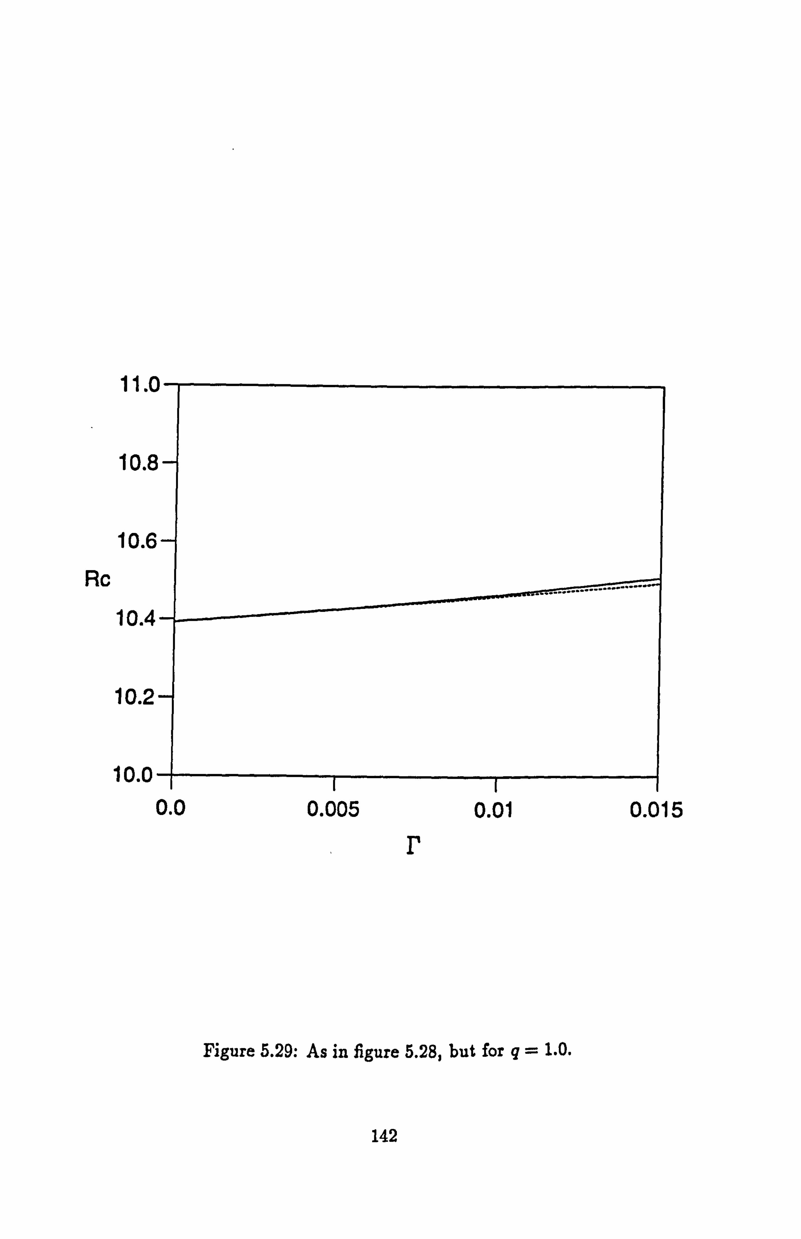
11.0
10.8
10.6
Rc
10.4-
10.2-
10.0-
r
Figure 5.29: As in figure 5.28, but for q=1.0.
142
0.0 0.005 0.01 0.015

10.8
10.7
10.6
Rc 10.5
10.4
10.3
10.2
r
Figure 5.30: As in figure 5.28, but for q= 10.0.
143
0*100 2*104 4*10-A

R=R2(r). (5.51)
It is expected that (5.50) will be a linear approximation to these curves close to the F=0 axis. Figures 5.28,5.29 and 5.30 show plots of (5.50) and (5.51) close to the I' =0 axis for the cases
q=0.1,1.0,10.0.
The figures show that (5.50) is indeed a linear approximation to the exact, nu- merically calculated critical Rayleigh numbers for the second most unstable mode, provided that r is small. This confirms that the solution (5.48) is the analytic form of the second most unstable linear perturbations for small values of r. These
results confirm the accuracy of the numerical method used in chapter 5.
144

Chapter VI
The Nonlinear Regime
6.1 The Nonlinear Equations
To investigate the nonlinear regime that develops from the linear solutions found in chapter 5, the nonlinear terms neglected in the linear problem are re-
stored to the governing equations. This has two main consequences. Firstly, these
nonlinear terms lead to the formation of new harmonics in the x and y directions.
The interaction of these new harmonics with each other produces the nonlinear behaviour that is investigated here. Secondly, Taylor's constraint is not in general
satisfied in the nonlinear regime. The Maxwell stress generated by the nonlinear
solutions leads to the acceleration of a geostrophic flow though Ekman suction at the boundaries. Because the shear generated by this flow is responsible for equi- librating the amplitude of the solutions, they are called Ekman solutions. The
importance of these Ekman solutions lies in the fact that they may evolve in such
a way that Taylor's constraint becomes satisfied. Of key importance is finding
whether this occurs, and if so, how Taylor's constraint comes to be satisfied.
For geophysical values of q, namely
q «1,
the results of chapter 5 indicate that the exchange of stabilities is the preferred
mechanism of instability. For these values of q therefore, the nonlinear regime that develops from the linear solutions will be steady. For this reason, the oscillatory
case will not be considered, since it is not relevant to the Earth's interior.
145

Hence, solutions of the following equations are required
2aZ +nah =o, (6. la) y
FZ ý- A- (V2b) - RV2 0=o, (6.1b) 2
2w r
2V =ä ý2j (bxby)dzdy], (s. ýc)
Ob öw qv Z (6.14) ay= ay+Db,
L_ LC 2 d2V _
dV äbß 5bxll - a-/I'
(6.1e) 4V ay [iy+ E+g(bxdxz
dx (Lb
(6.11) Ve =w+V28,0Y
V, alb a 6.1vHbx = axax - ey, ( 9)
2 alb ýHby - äyöz + 8x'
, V2 Hux ö9xa2Wz äy OC (4.2i) --'
2 2 8uy H ayaz + äx
- (6.1j)
146

These are the nonlinear, time-independent equations governing the system. They
are to be solved subject to the usual boundary conditions,
w=b=Oz=0=0 on z=0, (6.2a)
w+ mV sin(my) =b+q sin(my) =ý=0- cos(my) =0 on z=a. (6.2b)
The solutions of (6.1) and (6.2) are assumed to take the form
00 X=>X. (z) exp(inlx + imy) + c. c., (6.3a)
n=-oo
00 V=E Vn exp(inlx) + c. c., (6.3b)
n=-OC>
where
{T(z) W, (z) A, (z) X, (z) Z. (z) Xn(z) =
Byn(z) Byn(z) U ..
(z) Üy, (z)], (6.4)
represents the z-structure of the nth harmonic, and the V, a are complex constants. It can be seen from (6.3) that the nonlinear terms only create new harmonics in the
x direction. This occurs because the nonlinear terms in the governing equations are those associated with the geostrophic flow, V. The y average in the mean Maxwell stress,
M= m2ý5j Bx By dzdy,
(which is used to determine V) has the effect of removing any new harmonics
created in the y direction. However, any new harmonics created in the x direction
147

will be retained. Since the product of V with any other quantity can therefore only
create x harmonics, there are no new y harmonics introduced into the problem
Substituting (6.3) into (6.1), equations are obtained for the z structure of the
nth harmonic and the nth coefficient of V. They are given by
2DWn + Aim,.. = 0, (6.5a)
2DZn - Aim(D2 - k. 2)B� + RknTT = 0, (6.5b)
2V n= rAginl {1f (BPBy,
P-n)dz}, (6.5c)
ao
00 (D2 - kn)B� + imW, ý _ gim(VP + V*p)Bn_p, (6.5d)
P=-00
(D2 - kn)Xn + imZn =? q(VP + V*P) IimXn_p + pn12By, n-P - PlmBy, n-P], P=-o
L
(6.5e)
00 (D2 - kn)TT + Wn =E im(Vp +V *p)Tn-P, (6.5f)
P=-00
knBxn, = inlDB,, + imXX, (6.5g)
nBgn = imDBn - inlX,,, (6.5h) k2
k2Uxn = inlDWn + imZn,, (6.5i)
knUUn = imDWW, - inlZn, (6.5j)
148
where D= and g-z
kn = n212 + m2.
Substituting (6.3) into (6.2), the boundary conditions become
W,, =B, a=DX,, =T, a=O on z=0, (6.6a)
Wn - t2 (Vn +V_*n){1- bpn} = Bn -
2Q bon = DXn = Tn - 2bpn
=0 on z= 7r, (6.6b)
where bnm is the Kronecker delta. The form of the boundary conditions on the top boundary is indicative of the fact that different effects are forcing different harmonics. It is the interaction of the geostrophic flow V with the bumps that forces the oblique (n L 0) harmonics, while the distortion of the isotherms and vertical magnetic field by the bumps forces the transverse (n = 0) harmonic.
6.2 Non-Uniqueness Of Solution
Equations (6.5) and (6.6) are invariant under the transformation
0 X 1, (6.7)
where 0 is a real constant. This reflects the fact that the layer is invariant under translation in the x direction. Because of this, solutions of (6.5) and (6.6) are not
unique. If
00 X= S X�(z) exp(inlx + imy) + c. c.,
n=-oo
00 V= >Vn exp(inlx) + c. c.,
n=-oo
is a solution of (6.5) and (6.6), then so is
149

Xp ={ exp(in0)X,, (z)} exp(inlx + imy) + c. c., n=-oo l
00 Vo =E{ exp(inI)Vn } exp(inlx) + c. c..
n=-ao lJ
To obtain unique solutions, the arbitrary phase i must be fixed. This is done as follows.
Recall that the z-structure of the basic state obeys the conditions (4.21),
namely
TO= . 'ö ,
Uzo = -U: 0,
Uyo =- Uyo,
Wo=wo,
Bxo = Bxo
Byo = B* YO)
Bo = -Bo *l
Xo = -X 6)
Zo = Zö.
150
Since the arbitrary phase does not effect the transverse (n = 0) harmonic, it can be assumed that the transverse harmonic continues to obey (4.21) in the nonlinear
regime. However, by imposing (4.21) on the transverse harmonic, it transpires that
the coefficients of the nonlinear harmonics obey the following conditions.
Tn n even, Tn =
T. n odd,
-u: n odd, Uzn, _
Uz*n n even,
1-Uyn n odd, Uyn
Uy*n n even,
W� n even, Wn =
-Wn n odd,
Bxn n even, Bxn =
I -Bin n odd,
Byn n even, Byn _
-Byn n odd,
n odd, In Bn
B', n even,
-X;, n odd, X, =
Xn n even,
151
(6.8a)
(6.8b)
(6.8c)
(6.8d)
(6.8e)
(6.8f)
(6.8g)
(6.8h)

Zn n even, Zn _ (6.8i)
-Z; * n odd.
That is, each unknown is either purely real or purely imaginary, depending on the value of n. (Note that (6.8) is also consistent with the conditions (5.47) obeyed by the perturbations found in chapter 5). By imposing (6.8) on the nonlinear solutions, the arbitrary phase the x direction will be fixed, and unique solutions will be obtained.
6.3 The Method Of Solution
The equations for the z structure of the nonlinear solutions form an infinite
set of coupled nonlinear ODE's. To solve the system numerically, it is necessary to truncate the solutions in such a way that a finite number of equations is ob- tained. This is done by approximating the infinite series (6.3) that define the exact solutions by finite series of the form
N X= Xn(z) exp(inlx + imy) + c. c., (6.9a)
n=-N
N V=> Vn exp(inlx) + c. c., (6.9b)
n=-N
where N is a positive integer. Under the approximation (6.9), only the 2N +1 harmonics
Xn(z), nE {-N, -N + 1, ..., N-1, N},
and the 2N +1 coefficients
V11, nE {-N, -N+1,..., N-1, N},
need to be determined. This is done by solving 2N +1 sets of coupled ODE's (one
set for each nE {-N, -N + 1, ..., N-1, N}) of the form
152

2DWn + AimXX = 0,
2DZ,,, - Aim(D2 - kn)B,, + RknT,, = 0,
N 2V,, = rAqinl {1 J"(B,,,, B, *, p-,,
)dzl, p_-N
T lp-n I <N
(DZ - kn)B, ý + imWn = N
gim(V, + V*p)B,, _p,
p=-N lp-nl<N
(6. ioa)
(6.10b)
(6. ioc)
(6.10d)
N [imXn_p (D2 - -I imZ_ pN
(V+ Vp) + pnl2Bx, n_p - plmBy, n-P] ip-ni <N
(6.10e)
(D2 - kn)Tn + Wn = N
E im(Vp + V*p)Tn_p,
p=-N fp-nl<N
(6. iof)
kn B.,, = in1DBn + imX,,,
k2By, a - imDBn - inlXn,
k2 nUx� = in1DWn + imZ,,,
knUyn = imDWn - inlZn.
(6.1Og)
(6.10h)
(6.10i)
(6.1Oj)
153

The boundary conditions applied for each value of n are given by
Wý=Bn=DX,, =T,,, =O on z=0, (6.11x)
im im Wn- 2 (Vn-ýV n){1-bon}-Bn-2
Son=DXn=Tn-2bon=0 on x=7. 4
(6.11b)
The solution of (6.10) and (6.11) will tend to the solution of the exact problem in
the limit N -º oo. Therefore, provided N is made large enough, (6.9) will be a good approximation to the exact solution.
Equations (6.10) and (6.11) can be solved numerically since they constitute a finite system of equations. This is done using the Tau method in the usual man-
ner. The harmonics to be determined are assumed to have the following spectral
expansions
TT(z)
Wn(z)
Bn(z)
X (z)
Xn(z) = Zn(z) _
B�(z)
BB, a(z)
Uzn(z)
Uyn(Z)
154
r LMÖZTnrPr(Z )
º EMö1 WnrPP(Z )
Y2MÜ2 BnrPr(x )
º EM+ZXnrPr(Z )
EMO ZnrPr(x )
r sr=O
BxnrPr(x )
LsMpl BynrPr(z )
º ýr=0 um� Pf (Z)
Mº ýr=o Uynr pr (Z)
(s. 12)
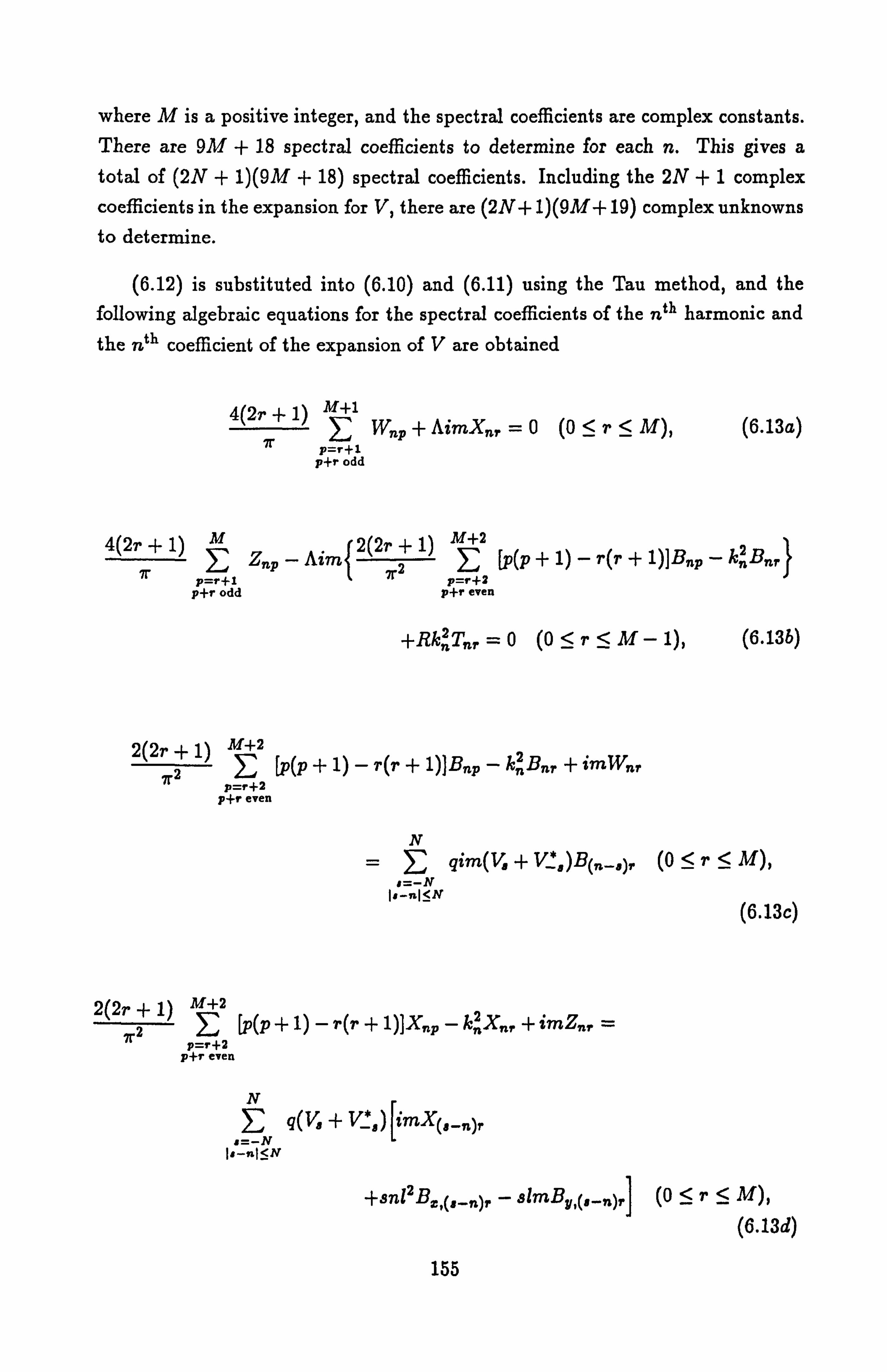
where M is a positive integer, and the spectral coefficients are complex constants. There are 9M + 18 spectral coefficients to determine for each n. This gives a total of (2N + 1)(9M + 18) spectral coefficients. Including the 2N +1 complex coefficients in the expansion for V, there are (2N+ 1)(9M+ 19) complex unknowns to determine.
(6.12) is substituted into (6.10) and (6.11) using the Tau method, and the following algebraic equations for the spectral coefficients of the nth harmonic and the nth coefficient of the expansion of V are obtained
4(2r + 1) M+1 E W, Z , + AimX,,, =0 (0 r< M), (6.13a)
7r p_r+l
-
p+r odd
4(2r + 1) M {2(2r+1) EZ [p(P+ 1) - r(r + 1)]Býp - k2Bnr Znp-Aim 7Z 7r
E} p=ri-1 p=r+2
p+r odd p+r even
+RknTnr 0 (0 <r<M- 1), (6.13b)
2(2r + 1) M+2 2
[p(P+1)-r(r+1)]Bnp-knBnr+imWnr p-r}2
p-fr even
N
=2 gim(V, + V*, )B(n_, ),. (05 r< M), #_-N
I. -nI<N (6.13c)
2(2r -} 1) M+2 Z
rzE [P(p + 1) - r(r +l )]Xnp - knXnr + imZnr =
y=r+a p+r even
N [iMX(8-n)r 4(V8 ý' V *a)
"=-N I s-nl<N
-Fsnl2Bx, (, _n),, - slmBy, (, _�)r] (0 <r< M),
(6.13d)
155

2(2r + 1) M+2 2
7r2 [p(p + 1) - r(r -I-1)]Tnp - knTnr -I- Wnr
p+r even
N
_ im(V, + V_ l)T(n_, ),. (0 <r< M),
a--N je-ni<N
(6.13e)
2(2r + 1) M+2 knBxn, = inl{ Bnr} + imX,,,. (0 <rCM+ 1), (6.13f)
P=r+1 p+r odd
2(2r + 1) M+2 k. 2By,
nr = im{ E BnP} - inlXn,, (0: 5 r: 5 M+ 1), (6.13g) p=r+1
p+r odd
f2(2r+1) M+' %ý, Üxýn, = inl E Wnp + imZn7 (0
_< r <_ M), (6.13h)
p_r+l p+r odd
2 2(2r -{-1) M+1
Wr} - in1Z,, r (0 <_ r< M), (6.13i) knUy, nr - imI E p=r+i p+r odd
(6.13j) Nf E1 Bx " Bv, ( ) 2Vn = I'Aginl l,
P e-n P!
#=-N r-o 2P +1 J'
Is-nl<N
M+1 (-1)PW1 = 0, (6.13k)
p=0
E1 Wnp
im(vn -f- V`n)(1- bon)) (6.131)
r=o 2
156

M+2 E (-1)PT�p = 0, (6.13m) p=0
M+2 E T., = 2bo,,, (6.13n) p=O
M+2 E (-1)"B�. p = 0, (6.13o) p=0
M+2 B,., =
2q bon., (6.13p) P=o
M+2 E (_1)p+lp(p + 1)Xnp = 0, (6.13q) p=0
M+2 Z p(p + 1)Xnp = 0. (6.13r) p=0
(6.13) defines 9M+19 algebraic equations for each value of n. Therefore, a total of (2N + 1)(9M + 19) complex algebraic equations in the (2N + 1)(9M x-19) complex unknowns is obtained. This corresponds to a system of 2(2N + 1)(9M + 19) real equations in 2(2N + 1)(9M + 19) real unknowns.
However, applying (6.8) to eliminate the arbitrary phase in the x direction, it can be seen that exactly half of these unknowns are trivially zero, since each coefficient is either purely real (no imaginary part) or purely imaginary (no real part). Setting the relevant real or imaginary parts of each coefficient to zero to
satisfy (6.8) leaves a system of (2N + 1)(9M + 19) real algebraic equations in (2N + 1)(9M + 19) real unknowns. These nonzero unknowns are all that are necessary to define the coefficients of the expansions of each harmonic and the
coefficients of the geostrophic flow.
The algebraic equations for the coefficients of the expansions are solved using NAG routine CO5NCF. To use this routine, it is necessary to input an initial
guess for the values of the unknowns. The routine then uses a modification of the Powell hybrid method to find the exact solution from this guess. The correction
157

to the guessed solution at each iteration is found from a convex combination of the Newton-Raphson and scaled gradient directions. Under reasonable conditions, this ensures global convergence for solutions far from the exact solution and fast
convergence rates. In practice however, it is necessary for the guess to be close to the exact solution in order for the routine to converge.
6.3.1 Parameter Values
In order to solve the equations, values must be assigned to the parameters of the problem, namely A, q, i, m, r and R.
The case
A=41 q=1.0, (6.14)
will be used exhaustively to discuss the results. Although the value of q lies
outside the geophysical limit, it does lie in the region of the (q, A) plane where the
exchange of stabilities is the preferred mechanism of instability, so the results will be applicable to the core. The value of q is also large enough to avoid any of the
numerical problems associated will small values of q. The wavenumbers I and m
are chosen to be the critical wavenumbers derived in chapter 5. That is, they are taken to be
l= 2- 2,
m= 2
(6.15)
Three values of I' are chosen, namely
I' = 0.1,1.0, and 10.0. (6.16)
This ensures that a large range of values of r is covered. Finally, the equations are solved over a range of values of the driving parameter R.
6.3.2 Finding Nonlinear Solutions
To find nonlinear solutions, an initial guess at the solution of equations (6.13) is
required. To obtain this guess, consider the solutions of the linear stability problem
158

described in chapter 5. For the parameter values considered, the solutions of the linear stability problem have the form
X= bX*_1(z) exp(-ilx + imy) + Xo(z) exp(imy)
+SX1(z) exp(ilx + imy) + c. c., (6.17)
where 5 is an arbitrary parameter, which in chapter 5 defined the size of the
perturbations, and was there assumed to be small. Associated with (6.17) is a
critical Rayleigh number R,, at which the basic state loses stability to the linear
perturbations.
Now, (6.17) can be written more compactly in the form
1 X=
{s1hhl(z)} exp(inlx + imy) + c. c., (6.18)
n=-1
where
X-1(z) = X* i(z),
Xo(z) = Xo(z), X1(z) = Xl(z)"
Recall from chapter 5 that the 94(z) are determined numerically using the Tau
method, based on a truncation in the z direction of
M=7.
This numerical solution for the z structure of (6.18) will be used as an initial guess for the solution of the N=2, M=7 nonlinear equations at values of R just
greater than (or just less than) R,, the critical Rayleigh number associated with (6.18).
However, in addition to the desired N=2, M=7 nonlinear solution is the
solution given by
X=- Xo(z) exp(imy) + c. c., V=0, (6.19)
159

where Xo(z) is the solution of equations (4.6). This solution defines the basic state
at R. To prevent the NAG routine from taking the initial guess onto the basic
state, the parameter b is varied until convergence to the required N=2, M=7
nonlinear solution is found. This nonlinear solution can then be used as a guess for solutions at higher values of N and M.
6.3.3 Truncation Analysis
It is necessary to find values for N and M so that the nonlinear solution is
converged, i. e. so that any increase in N or M has no effect upon the solution. Now, it transires that the value chosen for M in the linear problem, namely
M=7, (6.20)
is also a valid choice for the nonlinear problem. Increasing M to eight has no effect
upon the following truncation analysis. To find how many harmonics are needed to achieve convergence, the meansquare value of the geostrophic flow,
< V2 >= 51 JoT V2dx,
is computed at a fixed value of the Rayleigh number. Using (6.9b) and performing the integration, it turns out that
N VZ >= IVn +V*. 12. (6.21)
n=-N
This quantity is calcuated for various N at the point
R= 11.051,
and the following convergence table is obtained
160

N <V2> 2 0.4687013 3 0.3784930 4 0.3792582 5 0.3752553 6 0.3743778 7 0.3743484 8 0.3743424 9 0.3743413
Table 6.1
This table shows that the solution does indeed converge as N is increased. It was decided to choose a truncation of
N=6, (6.22)
since this gives an accuracy of 5sf, which is precise enough for most purposes. This truncation gives thirteen harmonics in the x direction and requires the solution of 1088 nonlinear, algebraic equations in 1088 unknowns.
6.4 The Results
The amplitude of the nonlinear solutions will be defined by two quantities. The first of these is the meansquare heatflux generated by the nonlinear solution on the bottom boundary. This is defined as usual by
MI jYjm2(xyO)2dydx ZH
,
where F is the heatflux,
N
.ý_ zB =E DTn(z) exp(inlx + imy) + c. c..
n=-N
Performing the relevant integrations it turns out that
161

g= 72
EN +2 IZ (_1)P+ip(p + 1)TnpI2 (6.23)
n=-N p=O
The second quantity used to define the amplitude of the nonlinear solution is the
meansquare value of the geostrophic flow V, and is given by
N
< VZ >= EI vn + V*nI2. (6.24) n=-N
H and < V2 > will be plotted against the Rayleigh number, for each solution found. The results for the three values of r considered will be discussed seperately.
6.4.1 The Case r=0.1
Figure 6.1 shows the bifurcation structure of the nonlinear solutions when I' = 0.1. It is a plot of H over the complete range of R considered in this case. The dashed curve (- - -) represents the basic state. It is the meansquare heatflux
generated at the bottom boundary by the transverse roll forced by the bumps (as
computed in chapter 4). All the other curves in this figure represent nonlinear solutions.
The solid curve (-) represents the nonlinear evolution of the most unstable linear solution found in chapter 5. Figure 6.2(a) shows an enlargement of figure
6.1 close to the bifurcation point of this solution, while figure 6.2(b) shows the
amplitude of the geostrophic flow associated with the solution. The bifurcation is
subcritical, and occurs at the point Rc(l) = 10.3923, (which is the critical Rayleigh
number associated with the underlying linear solution). Because the bifurcation is
subcritical, the solution exists for values of R less than those predicted by linear
stability theory. In fact, the solution exists for 10.3053 <R< 10.3923. For
each value of R on this range, two solutions exist, one with a higher value of H
than the other. The larger amplitude solutions constitute the upper branch of the graph. Figure 6.2(a) shows that as R in increased from R= 10.3053, the
amplitude of the solution on the upper branch diverges, becoming infinite at the
point RTi) = 10.3923. Figures 6.2(b) and 6.3 (which show plots of < V2 > against R and H respectively) show how the amplitude of the geostrophic flow adjusts as the solution becomes unbounded. Together, they imply that
162

<V2>-º0 as RTRTlý.
This is the Malkus-Proctor scenario (Malkus and Proctor 1975). The geostrophic flow adjusts it's amplitude in such a way that it's influence on the magnetic field through the induction equation can enable the field to satisfy Taylor's constraint. In this case, it adjusts it's amplitude to zero as RT (1) (see figure 6.2(b)). Because V is zero at R= RTI), the condition
5[- j'T(bzb)dzdyJ=O
at R= RTlý,
is (trivially) satisfied, and so a Taylor state exists at R= RTl). The amplitude of the nonlinear solution becomes unbounded as the Taylor state is approached because the shear which equilibrates the solution vanishes with the geostrophic flow, and there is then nothing to control the amplitude of the solution, which increases without bound.
This solution is a Type I Ekman solution, as defined by Soward and Jones (1983). Solutions exhibiting this behaviour have been observed in various models of kinematic dynamos incorporating a geostrophic nonlinearity (see for example lerley 1985; Hollerbach and Ierley 1991; Barenghi and Jones 1991 for the a2 case, and Abdel-Aziz and Jones 1988 for the aw case).
The Taylor state at R= . 41) is itself interesting. As RT RTl), the amplitude
of the +1 harmonic begins to diverge to infinity, while the amplitudes of the other oblique harmonics all decay to zero. The Taylor state consists of a large amplitude (+)-roll (in the notation of chapter 3), together with the finite amplitude transverse
roll forced by the bumps. They are aligned in such a way that that Taylor's
constraint is satisfied. This Taylor solution can be identified with the single (-º-)-
roll Taylor solution obtained by Roberts and Stewartson (1974).
The dotted curve (..... ) on figure 6.1 shows the nonlinear evolution of the
second most unstable linear solution found in chapter 5 (i. e. the solution with the
second largest growth rate). This solution is shown more clearly in figure 6.5. It
consists of three branches: a lower branch (labelled a), an upper branch (labelled b) and a middle branch (labelled c). Figure 6.6 is a plot of the geostrophic flow
amplitudes associated with each branch close to the points where branches b and c bifurcate off branch a.
163

Figure 6.7(a) shows an enlargement of figure 6.1 in the region of the bifurcation
of branch a off the basic state, while figure 6.7(b) shows the geostrophic flow
amplitude associated with branch a. The bifurcation of branch a is subcritical,
and occurs at RP) = 13.3230, (which is the critical Rayleigh number associated
with the underlying linear solution), and the solution again exists for values of R
less than those predicted by linear stability theory.
As R is decreased from R<z), the amplitude of V adjusts it's value in such a
way that this solution evolves towards a Taylor state at RTZý = 10.3923. It does
this exactly as previously: the amplitude of V decays to zero, removing the shear
which equilibrates the solution, and therby allowing the amplitude of the solution to diverge to infinity. However, as V is zero at R= RT2ý, Taylor's constraint is
satisfied, so the solution satisfies
2a [2 mIm/ (bZby)dzdy] =0 at R= RTZ).
The Taylor state for this solution is different to the Taylor state found in the
previous case, even though both Taylor states exist at the same value of R. In
this case, as R I. RT2), it is the amplitude of the -1 harmonic that diverges to
infinity, while the amplitudes of the other oblique harmonics all decay to zero. This Taylor state therefore consists of a large amplitude (-)-roll, together with the finite amplitude transverse roll forced by the bumps, aligned so that Taylor's
constraint is satisfied. It is the analogue of the other single roll Taylor solution (the (-)-roll Taylor solution) found by Roberts and Stewartson (1974).
Figure 6.9(a) is an enlargement of figure 6.1 in the region of the bifurcation of branch b off branch a, while figure 6.9(b) shows the amplitude of the geostrophic flow associated with branch b. The bifurcation occurs at R(3 = 10.4388 (see figure
6.6). At this point, the solution is still in an Ekman state, although it is close to the
Taylor state on branch a. The solutions on branch b appear to evolve to another, different Taylor state at the point RT(2) = 10.8698. The Malkus-Proctor mechanism
allows the geostrophic flow to adjust so that it's influence on the magnetic field is
precisely that which enables Taylor's constraint to be met. In order to do this, the
geostrophic flow adjusts its amplitude so that
< v2 >-4 0(1), 164

as the Taylor state is approached, i. e. there is still a finite geostrophic flow in the Taylor state. In the Taylor state, V is determined implicitly by the requirement that it's effect on the magnetic field be precisely that which is needed to satisfy Taylor's constraint: it is no longer determined through Ekman suction. Malkus
and Proctor (1975) call aV thus determined an eigenflow. As the eigenflow gets selected by the solution, and Taylor's constraint becomes satisfied, the nonlinearity of the problem (the Taylor integral) vanishes. Once this occurs, the amplitude of the nonlinear solution can no longer be determined, and the solution becomes
unbounded.
However, despite the fact that the amplitude of the solutions on branch b are diverging to infinity, it is not clear whether the geostrophic flow is becoming an eigenflow - the amplitude is clearly continuing to grow as the amplitude of the
solutions on branch b diverge (see figure 6.9(b) for details). Therefore, it is not possible to say with any certainty whether this is a Taylor state, or whether the
solution is not fully converged on branch b. Given that the solutions on branch b are already of quite large amplitude, it seems that the latter is probably the
case. It could probably be shown that this is indeed a Taylor state, and that an
eigenflow is being selected, by increasing the truncation of the solution on branch
b. However, this was not done, as the computing power necessary to do this was
not available. Hence, we treat the solutions on branch b with caution, as it seems likely that the solution is not fully converged there.
Figure 6.10(a) shows an enlargement of figure 6.1 in the region where the final
branch of this solution lies. This is branch c. The geostrophic flow amplitude
associated with branch c is shown in figure 6.10(b). Branch c bifurcates off branch
a at the point R(c4) = 10.4744 (see figure 6.6). No Taylor solutions were found
on branch c. As R is increased from R(4), the solutions on branch c remain in an Ekman state, their amplitudes controlled by the shear generated by the geostrophic flow. Branch c comes to an end at the point Rcbl = 18.9771, where it bifurcates
onto the last nonlinear solution considered, which is shown as the double dashed (- -) curve in figure 6.1. Figures 6.11(a) and 6.11(b) show how branch c bifurcates
onto this solution.
The nature of the bifurcation may be understood as follows. As RT . fl) the
amplitudes of the harmonics of the solutions on branch c that are not of the form
exp(3inlx + imy),
165

500
400
300
H
200
100
0
R
Figure 6.1: The bifurcation structure of the nonlinear solutions for the case r=0.1. The curve (- - -) is the basic state, while all the other curves represent nonlinear solutions.
166
10 12 14 16 18 20
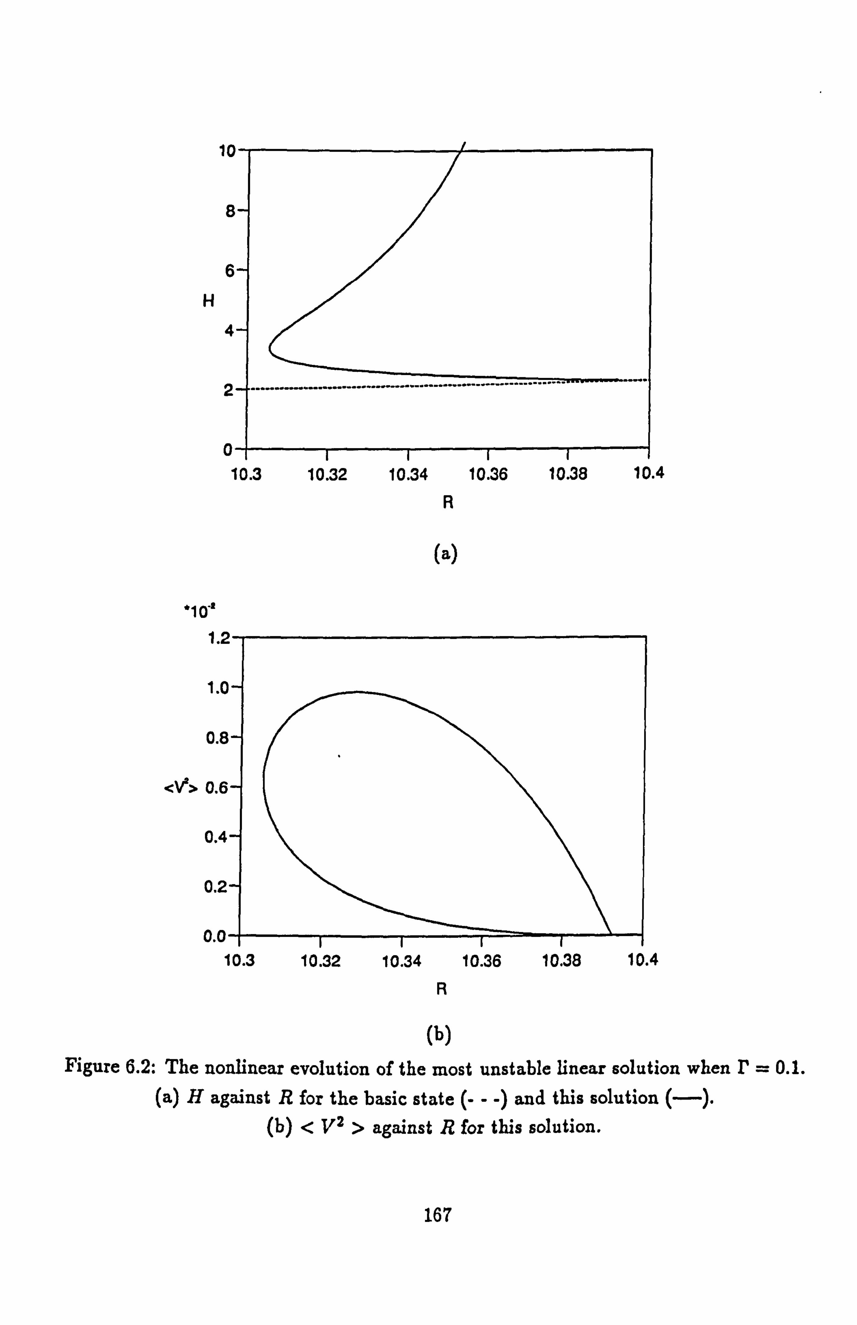
lo--
8-
6- H
4
2
10.3 10.32 10.34 10.36 10.38 10.4
R
(a)
*10-: 1.2
1.0
0.8-
<V2> 0.6-
0.4-
0.2-
0.0
10.3 10.32 10.34 10.36 10.38 10.4
R
(b)
Figure 6.2: The nonlinear evolution of the most unstable linear solution when r=0.1. (a) H against R for the basic state (- - -) and this solution (-).
(b) < V2 > against R for this solution.
167

0.015
0.01
<v2>
0.005
0.0
H
Figure 6.3: A plot of < V2 > against H for the first nonlinear solution when r 0.1.
168
0 50 100 150

X
V(x)
(a)
X
V(x)
(b)
Figure 6.4: Geostrophic flow profiles for the first nonlinear solution for r=0.1
when (a) R= 10.3823 and, (b) R= 10.3458, on the upper branch of the solution.
169
-0.1 -0.05 0.0 0.05 0.1
-0.2 -0.1 0.0 0.1 0.2

500
400
300
H
200
100
0
R
Figure 6.5: The nonlinear evolution of the second most unstable linear solution when r=0.1. H against R for the basic state (- - -) and this solution (--).
170
11 12 13 14 15 16 17 18

0.5
0.4
0.3
<v2>
0.2
0.1
0.0
R
Figure 6.6: The bifurcation of branches b and c off branch a when I' = 0.1.
171
10.4 10.5 10.6 10.7

100
80
60
H
40
20
0
I1
º1 1I
/I 1I
I 1 11
11
11 I
1º
i i
11 12 13 14
R
(a)
<v2>
10.5 11.0 11.5 12.0 12.5 13.0 13.5
R
(b)
Figure 6.7: An enlargement of branch a of the second nonlinear solution when r=0.1. (a) H against R for the basic state (- - -) and branch a (-).
(b) < V2 > against R for branch a.
172
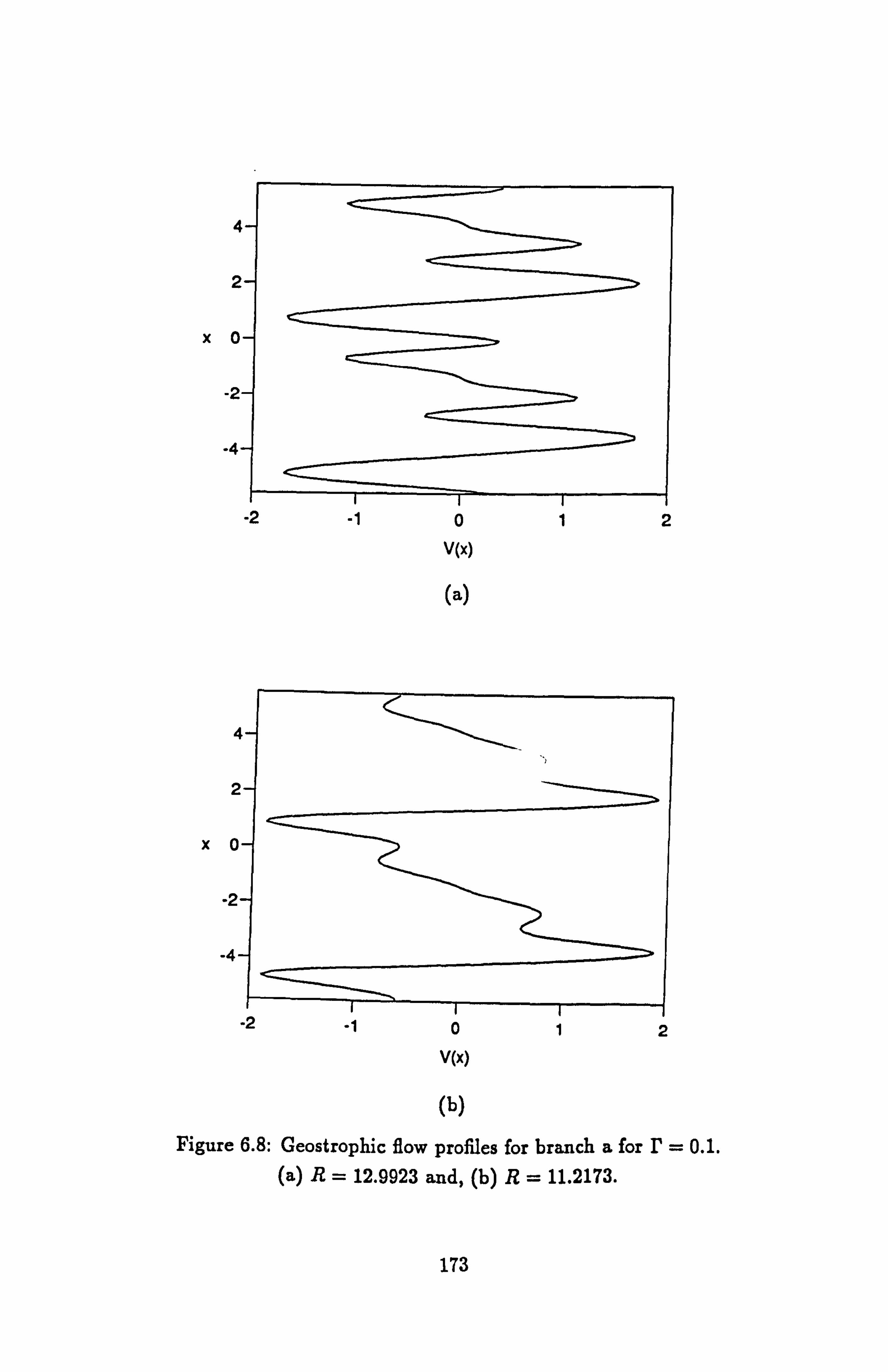
4
2
x
-2 -1 012 V(x)
(a)
X
(b)
Figure 6.8: Geostrophic flow profiles for branch a for r=0.1. (a) R= 12.9923 and, (b) R= 11.2173.
173
012
V(x)

70(
60C
H 500
300
5
4
3
<v2> 2
1
A
400
10.4 10.5 10.6 10.7 10.8 10.9 11.0
R
(a)
10.4 10.5 10.6 10.7 10.8 10.9
R
(b)
Figure 6.9: An enlargement of branch b of the second nonlinear solution when r=0.1. (a) H against R for branch b.
(b) < V2 > against R for branch b.
174

500
400
300
H
200
100
I' 11 12 13 14 15 16 17 18
R
(a)
8
6
4
2
F. 11 12 13 14 15 16 17 18 19
R
(b)
Figure 6.10: An enlargement of branch c of the second nonlinear solution when I' = 0.1.
(a) H against R for the basic state (- - -) and branch c (-).
(b) < V2 > against R for branch c.
175

65
60
55
H
So-
45-
40 18.5 18.6 18.7 18.8 18.9 19.0 19.1
R
(a)
<V2>
R
(b)
Figure 6.11: The bifurcation of branch c onto the solution (6.25) when r=0.1.
(a) The curve (--) is branch c, while (- -) is (6.25).
(b) as in (a) but showing < V2 >.
r
176
18.95 19.0 19.05 19.1

X
V(x)
(a)
X
V(x)
(b)
Figure 6.12: (a) Geostrophic flow profile for branch b at the point R= 10.7299 when r=0.1 (b) Geostrophic flow profile for branch c at the point R= 14.9926 when r=0.1.
177
-6 -4 -2 0246
-6 -4 -2 0246

1
11
H
0
n
18.95 19.0 19.05 19.1 R
(a)
0.
o. <v2>
o. 1
18.95
R
(b)
Figure 6.13: The nonlinear evolution of the solution (6.25) when r=0.1. (a) H against R for the basic state (- - -) and this solution (--).
(b) < V2 > against R for this solution.
178
19.0 19.05 19.1
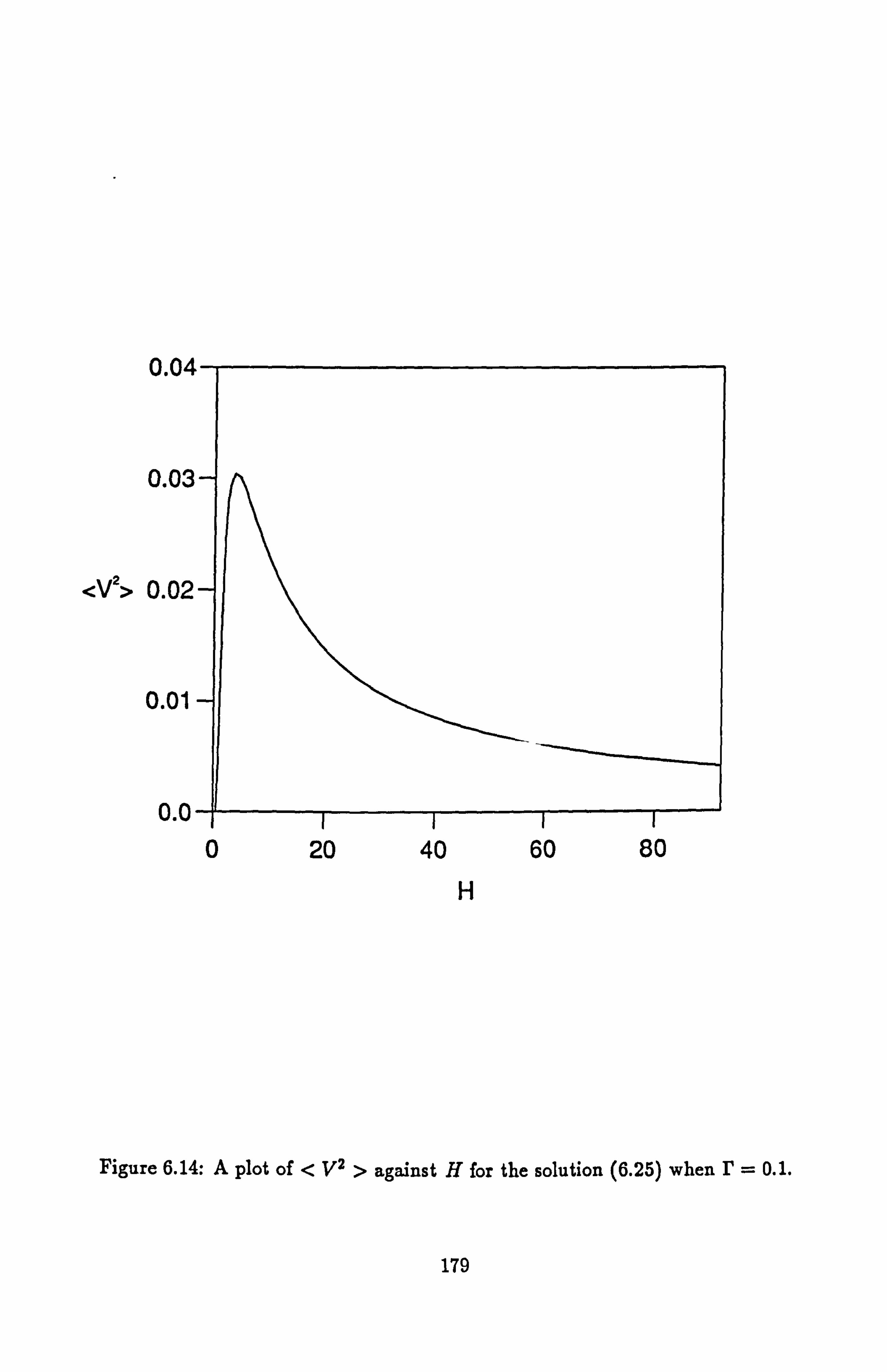
0.04
0.03
<V2> 0.02
0.01
0.0
H
Figure 6.14: A plot of < V2 > against H for the solution (6.25) when r=0.1.
179
0 20 40 60 80
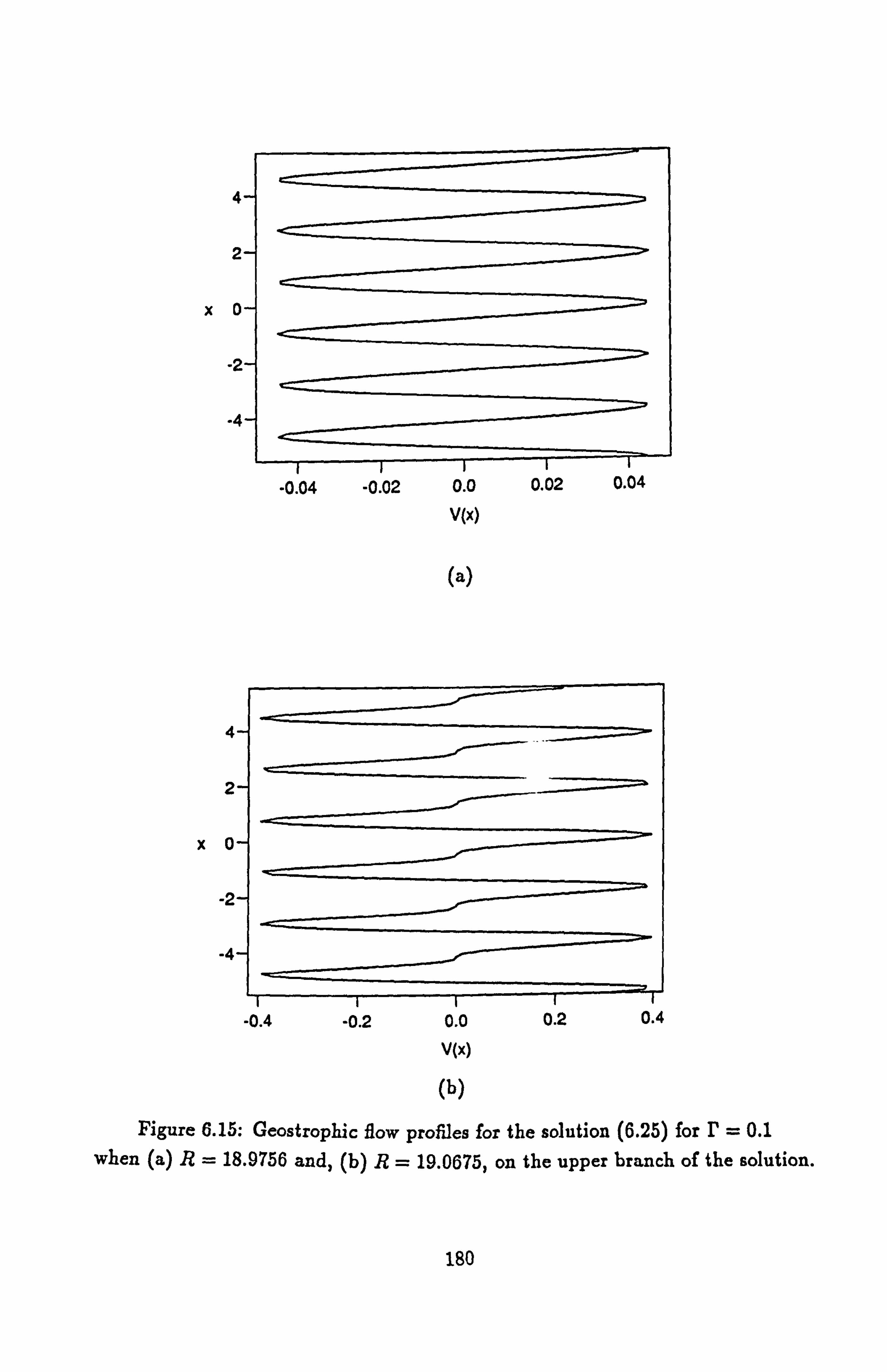
4
2
x0
.2
-4
V(x)
(a)
X
V(x)
(b)
Figure 6.15: Geostrophic flow profiles for the solution (6.25) for r=0.1
when (a) R= 18.9756 and, (b) R= 19.0675, on the upper branch of the solution.
180
-0.04 -0.02 0.0 0.02 0.04
-0.4 -0.2 0.0 0.2 0.4
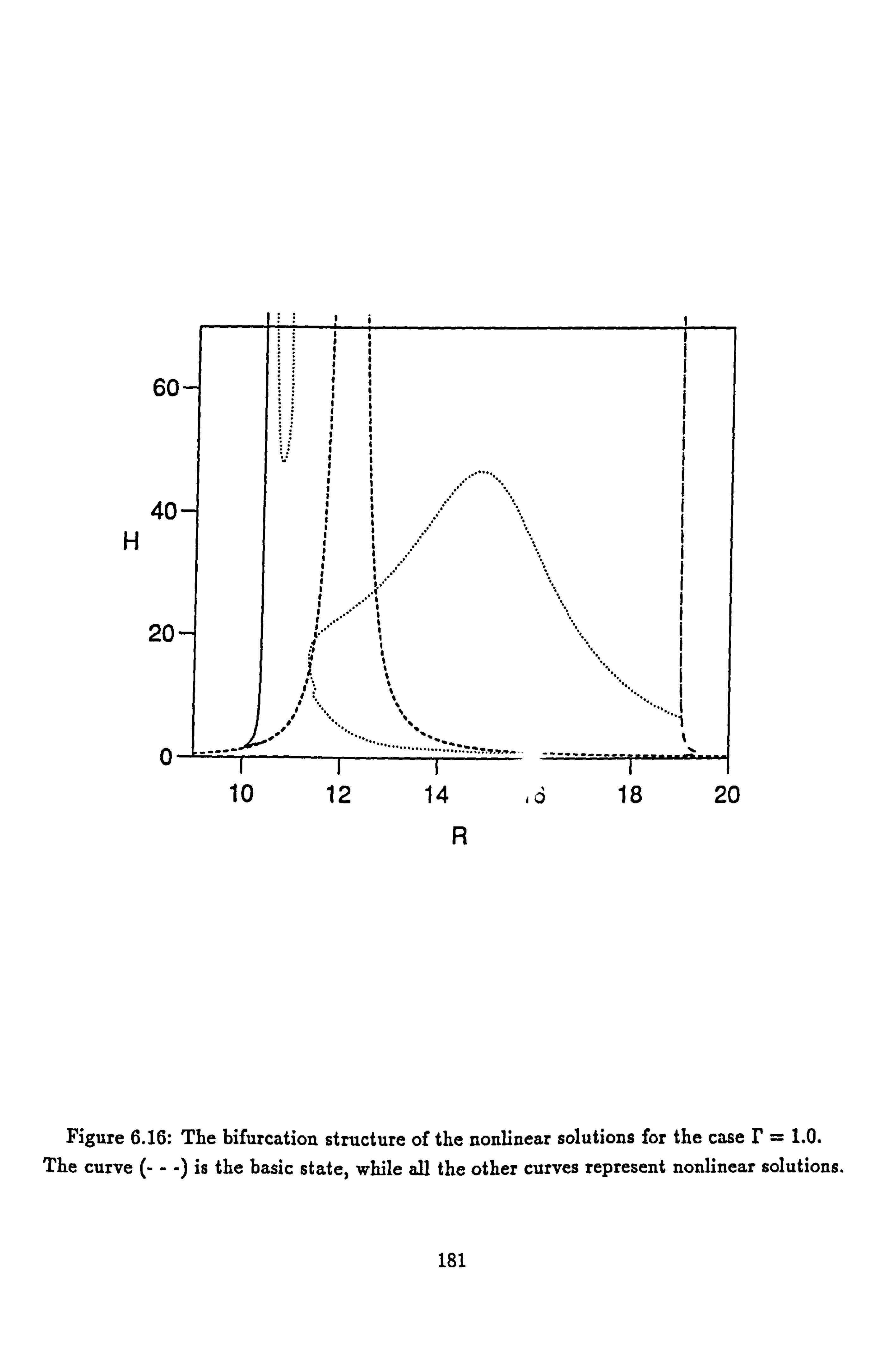
6C
40 H
20
0
R
Figure 6.16: The bifurcation structure of the nonlinear solutions for the case r=1.0. The curve (- - -) is the basic state, while all the other curves represent nonlinear solutions.
181
10 12 14 1ö 18 20
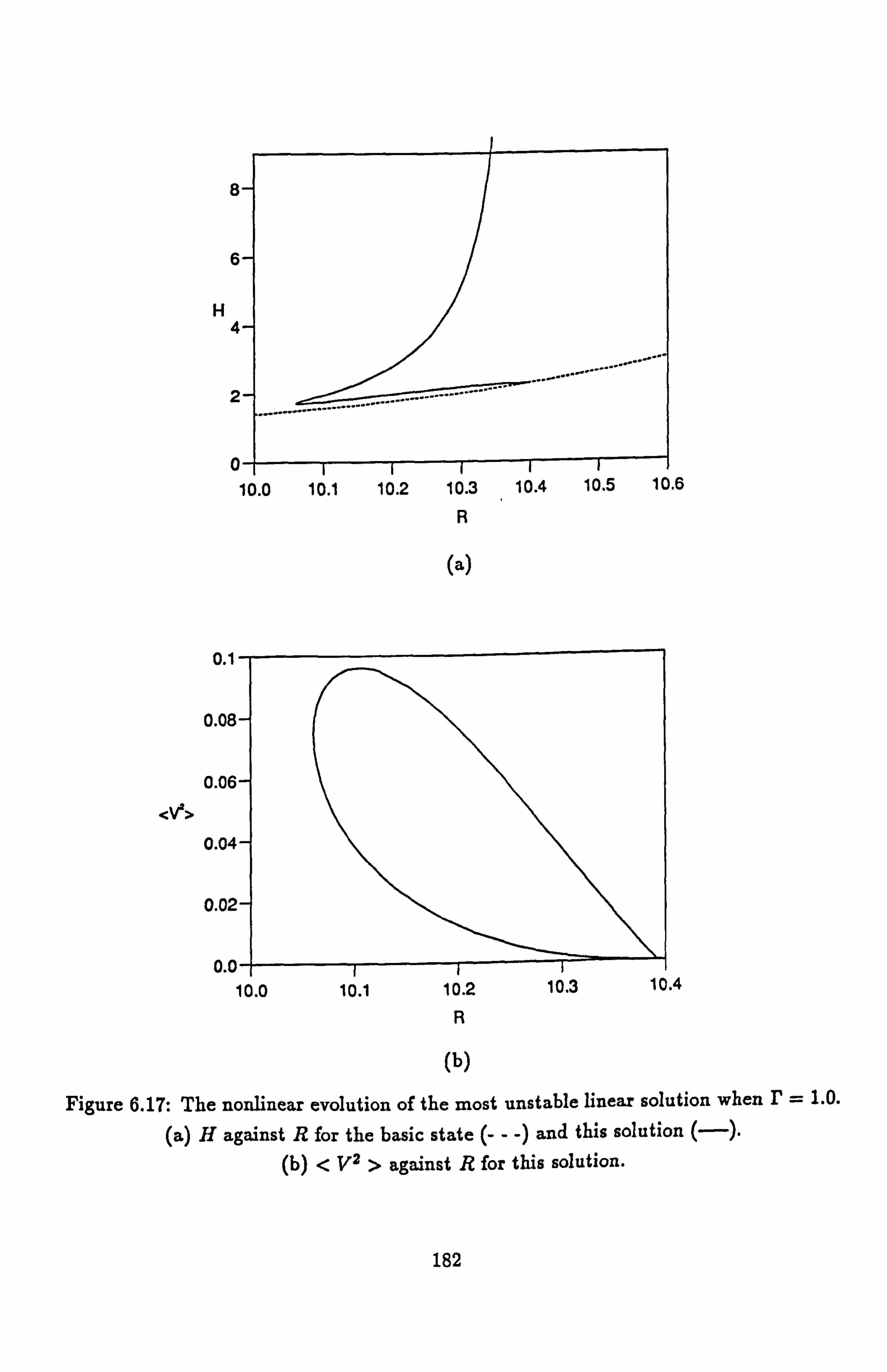
6
H 4
2-
07 10.0 10.1 10.2 10.3 10.4 10.5 10.6
R
(a)
0.1
0.08
0.06
0.04
0.02
0.0 10.0 10.1 10.2 10.3 10.4
R
(b)
Figure 6.17: The nonlinear evolution of the most unstable linear solution when r=1.0.
(a) H against R for the basic state (- - -) and this solution (-).
(b) < V2 > against R for this solution.
182

0.1
0.01
0.0E <V2>
0.04
0.02
0.0
H
Figure 6.18: A plot of < V2 > against H for the first nonlinear solution when r=1.0.
183
05 10 15 20 25 30 35

x
V(x)
(a)
X
V(x)
(b)
Figure 6.19: Geostrophic flow profiles for the first nonlinear solution for r=1.0
when (a) R= 10.3458 and, (b) R= 10.1242, on the upper branch of the solution.
184
-0.3 -0.2 -0.1 0.0 0.1 0.2 0.3
-1.0 -0.5 0.0 0.5 1.0

60
40 H
20
0
R
Figure 6.20: The nonlinear evolution of the second most unstable linear solution when r=1.0.
H against R for the basic state (- - -) and this solution (-).
185
11 12 13 14 15 16 17 18

4
3
2
1
10.4 10.5 10.6 10.7 10.8 10.9 11.0
R
(a)
10-
8-
6-
4-
2-
0-- 11 12 13 14 15 16 17 18 19
R
(b)
Figure 6.21: The amplitude of the geostrophic flow associated with the second nonlinear
solution when r=1.0. (a) < V2 > against R for branch d, and (b) < V2 > against R for branch e.
186

X
-2 -1 012
V(x)
(a)
x
(b)
Figure 6.22: (a) Geostrophic flow profile for branch d at the point R= 10.7402 when r=1.0 (b) Geostrophic flow profile for branch e at the point R= 15.7313 when r=1.0 on the upper.
branch of the solution.
187
-0.6 -0.4 -0.2 0.0 0.2 0.4 0.6 V(x)
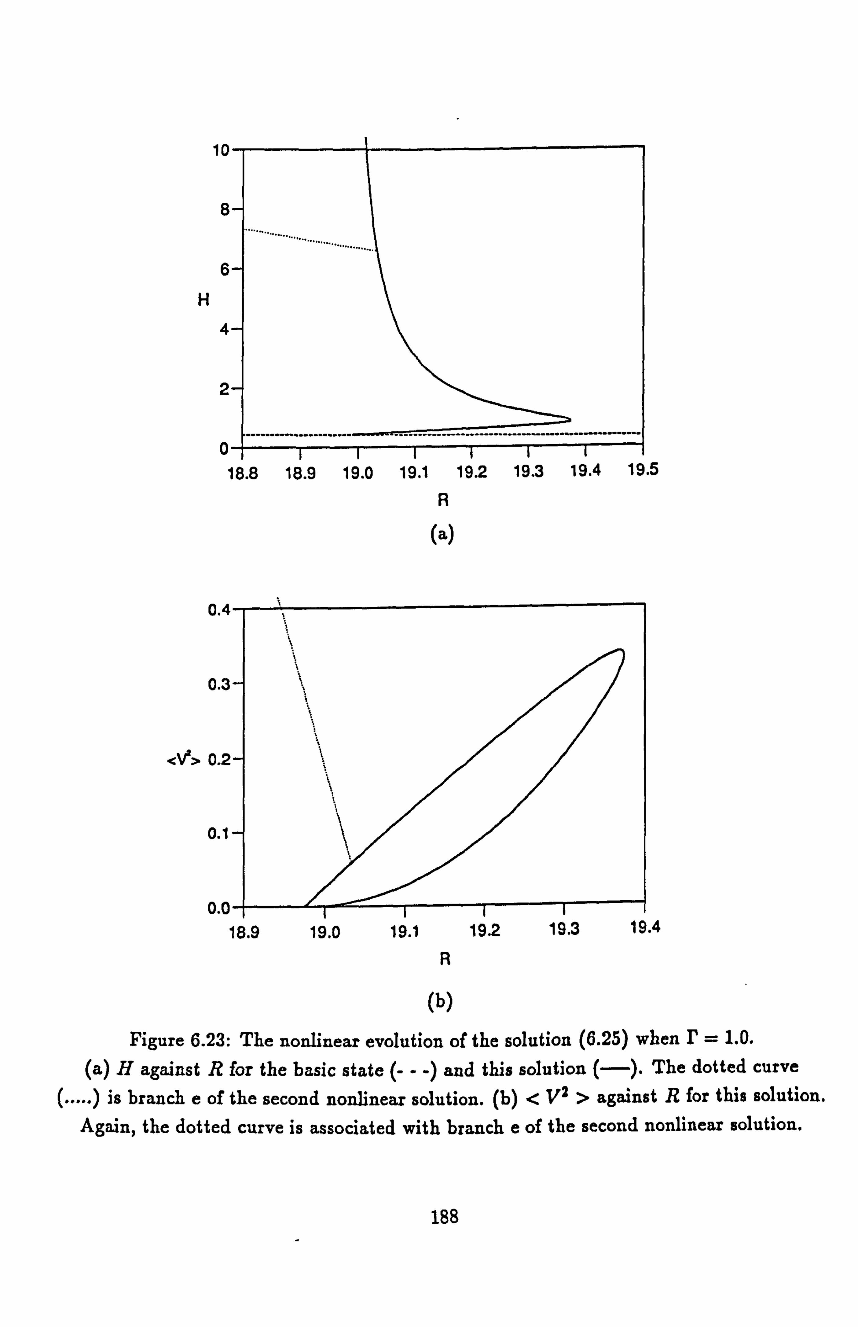
10
8
6
H
4
2
n
0.4
18.8 18.9 19.0 19.1 19.2 19.3 19.4 19.5
R
(a)
0.3
<V2> 0.2
0.1
0.0-j- 18.9 19.0 19.1 19.2 19.3 19.4
R
(b)
Figure 6.23: The nonlinear evolution of the solution (6.25) when r=1.0. (a) H against R for the basic state (- - -) and this solution (-). The dotted curve
(..... ) is branch e of the second nonlinear solution. (b) < V2 > against R for this solution. Again, the dotted curve is associated with branch e of the second nonlinear solution.
188

0.4
0.3
<V2> 0.2
0.1
0.0
H
Figure 6.24: A plot of < V2 > against H for the solution (6.25) when r=1.0.
189
05 10 15 20 25 30 35

X
V(x)
(a)
X
V(x)
(b)
Figure 6.25: Geostrophic flow profiles for the solution (6.25) for r=1.0
when (a) R= 19.1100 and, (b) R= 19.37444 on the upper branch of the solution.
190
1 0.0 0.5 1.0 -1.0 -0.5
-1.5 -1.0 -0.5 0.0 0.5 1.0 1.5

40
30
H 20
10
0
R
Figure 6.26: The bifurcation structure of the nonlinear solutions for the case I' = 10.0.
The curve (- - -) is the basic state, while all the other curves represent nonlinear solutions.
191
10 12 14 16 18 20 22 24

PAGE MISSING
IN ORIGINAL

At the point RýS), the solution has the form
N X= X3�(z) exp(3inlx + imy) + c. c., (6.25a)
n=-N
N V= V3,, exp(3inlx) + c. c., (6.25b)
n=-N
and the double dashed curve in figure 6.1 shows this solution. The region of the bifurcation of (6.25) is shown enlarged in figure 6.13(a), while 6.13(b) shows the
amplitude of the geostrophic flow associated with (6.25). These curves represent the nonlinear evolution of a linear solution of the form
1 {s11LIx3(z)} X=E exp(3inlx + imy) + c. c.. (6.26)
The major difference between the solution (6.25) and the others described is that the lenghtscale of the convection in the x direction has been made shorter by a factor of 3. This smaller scale convection is not the preferred mode of convection, that being given by the solutions described previously, and larger values of R are needed to force it.
The solution (6.25) bifurcates supercritically off the basic state at the point Rc( 6= 18.9752, which is the critical Rayleigh number associated with (6.26). The
solution exists for 18.9752 <R< 19.0661. For each value of R in this range, two solutions exist, one at a larger value of H than the other. The larger ampli- tude solutions constitute the upper branch of the graph shown in figure 6.14(a). The large amplitude solutions evolve to a Taylor state at RT 4)
= 18.9752 via the
same mechanism as the first nonlinear solution described. That is, the geostrophic flow amplitude decays to zero as R R4), removing the shear that controls the
amplitude of the solution, and allowing Taylor's constraint to be met at R= RT4).
The Taylor solution at R= RT4) consists of a (+3)-roll whose amplitude is diverging (the amplitude of the other oblique modes decaying to zero) together
with the finite amplitude transverse roll forced in the layer by the bumps. This
occurs because as RI RT4), the +3 harmonic dominates the solution, while the
amplitudes of the other oblique harmonics decay to zero.
193
6.4.2 The Case r=1.0.
Increasing the value of r leads to a stronger geostrophic flow through the
modified Taylor's constraint. The enhanced nonlinearity in this case suppresses the convection even more strongly, and as a consequence the amplitudes of the
nonlinear solutions for this case (and for larger values of I') are smaller.
Figure 6.16 shows the bifurcation structure of the nonlinear solutions obtained
when r=1.0. Each curve on the diagram represents the same solution as found
in the r=0.1 case. Hence, the dashed curve (- - -) represents the basic state, the
solid curve (-) is the nonlinear evolution of the most unstable linear solution, the dotted curve (..... ) represents the nonlinear evolution of the second most unstable linear solution, and the double dashed curve (- -) is the solution (6.25) for this
value of F.
As figures 6.17 and 6.18 show, the nonlinear evolution of the most unstable linear solution is qualitatively the same for r=1.0. The solution bifurcates
at the same point, Rýi) = 10.3923, and has a Taylor state at the same point, Rý1ý = 10.3923 as the r=0.1 case. The Taylor state, and the mechanism by which it is brought about are also similar. That is to say, the Taylor state consists of
a (+)-roll with diverging amplitude, together with the finite amplitude transverse
roll in the layer by the bumps.
The nonlinear solution (6.25) also behaves in a similar manner when r=1.0,
as figures 6.23 and 6.24 show, so it will not be discussed.
The major difference between the r=0.1 solutions and the r=1.0 solutions lies in the nonlinear evolution of the second most unstable linear solution. This
is the dotted curve in figure 6.16, which is shown enlarged in figure 6.20. Instead
of the three branch connected solution obtained previously, two distinct seperate branches are obtained, an upper branch (labelled d) and a lower branch (labelled
e). As r is increased from 0.1 to 1.0, branch a of the r=0.1 solution breaks
into two parts. It's large amplitude part combines with branch b of the r=0.1
solution to form branch d of this solution, while it's small amplitude part combines
with branch c of the r=0.1 solution to form branch e of this solution. The exact
value of r at which the break occurs has not been determined. The amplitude of the geostrophic flow associated with branch d is shown in figure 6.21(a), while that
associated with branch e is shown in figure 6.21(b).
194

The solutions on branch d of this solution are unusual in that they are not connected to the basic state in any way. Rather, branch d connects two (probable) Taylor states, one at RT2) = 10.3923 and the other at RTg) = 10.8787. The Taylor
state at R= RT) has it's origin in the Taylor state found on branch a of the r=0.1 solution. It consists of a (-)-roll with diverging amplitude (the amplitude of the other oblique modes decaying to zero), together with the finite amplitude transverse roll forced by the bumps, aligned so that Taylor's constraint is met. As figure 6.21(a) shows, there is no geostrophic flow associated with this Taylor
state. On the other hand, as RT RT3), the solution diverges to infinity and appears to enter a Taylor state. However, as figure 6.21(a) shows, the amplitude of the
geostrophic flow is now diverging as this occurs and so this result needs to be treated with caution. As in the r=0.1 case, it is very likely that the solution is not fully converged here, and an increase in the truncation of the solution is
required to clarify matters. Again, this was not possible as the computing power was not available.
The solutions on branch e bifurcate off the basic state at the point R( C2) 15.8313 (which is the critical Rayleigh number associated with the second most unstable linear solution when r=1.0). The bifurcation is subcritical, and so the solutions exist for values of the Rayleigh number less than those predicted by linear stability theory. Each solution on branch e is an Ekman solution - no Taylor
solutions were found. Branch e comes to an end at the point RP = 19.0230, where it bifurcates onto the nonlinear solution (6.25) in the same manner as described in the r=0.1 case: the amplitude of each harmonic that is not of the form
exp(3inlx + imy)
(where n is an integer) decays to zero as RT RC(s). It is interesting to see that the Taylor states for this solution (which lie on branch d) cannot be reached from the initial bifurcation of this solution (which occurs on branch e). This sort of solution, where the initial bifurcation is not connected to the Taylor states of the solution, has been seen before. Soward and Jones (1983) call this a type II Ekman solution. They have also been seen in models of kinematic dynamos (see for example Barenghi and Jones 1991, a2 case).
6.4.3 The Case I' = 10.0
The results for this value of r are shown in figure 6.26, which shows the bi-
195

furcation structure of the nonlinear solutions for this case. Since the behaviour of the solutions in the case I' = 10.0 is qualitatively the same as that of the r=1.0
case, they will not be discussed.
6.5 The Post Taylor Equilibrium
In each of the nonlinear solutions found in this chapter, the amplitude of the
solution diverged to infinity as Taylor's constraint became satisfied. This was the Malkus-Proctor scenario, where the geostropic flow evolved to the eigenflow whose
effect on the magnetic field through the induction equation was precisely that
needed to satisfy Taylor's constraint. As V evolves to this eigenflow, the nonlin-
earity of the problem (the Taylor integral) vanishes. The amplitude of the solution
cannot be determined once this occurs, and the solution diverges to infinity.
In the Taylor state, the solution is outside the asymptotic limit in which the
governing equations (6.5) are valid. To follow the solution further, all the nonlin-
earities neglected in the derivation of (6.5) must be restored to the problem. These
nonlinearities (e. g. the advective terms in the heat and induction equations) then
become responsible for equilibrating the solution. The solutions of the full problem
will also satisfy Taylor's constraint (having evolved through the Ekman states de-
scribed here). Such solutions have been found in models of kinematic dynamos (see
Abdel-Aziz and Jones 1988; Barenghi 1992a; Barenghi 1992b), but this procedure is not carried out here.
196

Chapter VII
Conclusions
The main theme of this work has been determining the effect of adding bumps
to a rapidly rotating fluid layer containing a strong azimuthal magnetic field. The
configuration of the layer is chosen so that the layer rotates about the vertical z direction, and has an applied magnetic field aligned in the horizontal y direction (which is chosen to represent the azimuthal direction in the core). Gravity is
chosen to act in the negative z direction, and thermal forcing is used to drive the
convection in the layer.
Since the main interest lies in isolating the key mechanisms by which the bumps
effect the convection, the bumps themselves are assumed to take a simple form,
namely a sinusoidal undulation which varies in the y direction. The axis of the bumps is chosen to be perpendicular to the applied magnetic field, and lies in the
x direction. Such a simple form of topography has also been used by Kelly and Pal (1977), Kuang and Bloxham (1993) and Bell and Soward (1995) as a model of the topography on the core mantle boundary.
The bumps are assumed to be small in the sense that the bump size parameter
y satisfies
ry«1.
To check that this is a valid assumption, -y must be calculated for the core. Taking
rCMB = 3481km, rICB = 1221km,
as the radii of the core mantle boundary and the inner core boundary respectively,
and assuming a bump height of tkm (see Hide 1967,1969), then
ry = 4.42 x 10⁻⁴, (7.1)
197
in the core. This value is certainly small enough to justify making the small bump
approximation.
In chapter 2 the equations governing the topographic convection in the layer
are derived from the full MHD equations governing convection in the core (i. e. the
magnetogeostrophic equations). The derivation makes use of the fact that 7 is
small, and neglects all terms of 0(72) or smaller from the problem. The resulting system of equations, namely equations (2.35), contain the parameter
E2 ý
which is a modified bump size parameter. r is the key parameter which measures the effect of the bumps upon the convection. It also arises in the non-magnetic
case (see Bell and Soward 1995; Bell 1994). In chapter 2, it is argued that r is a finite parameter. Again, this can be checked for the core using the values of -y and E in the core. These values give
I' = 19.53, (7.2)
which is certainly finite. r appears in the modified Taylor's constraint used to
determine the geostrophic flow. It has the role of measuring the strength of the
geostrophic flow, and hence, the effectiveness of the geostrophic nonlinearity in
equilibrating the convection.
The boundaries of the layer are assumed to be rigid, isothermal and perfectly
electrically conducting. The fact that y is small is used to simplify the boundary
conditions on the bumpy top boundary. These boundary conditions are Taylor
expanded in ry, and only the 0(1) and 0(7) terms are retained. In this way, a set
of inhomogeneous boundary conditions on z =, 7r is obtained.
The presence of the bumps distorts the horizontal applied magnetic field, cre-
ating a small correction b to the main magnetic field. This small correction ensures that the main magnetic field fits into the bumpy layer, and is also responsible for ac-
celerating the geostrophic flow through the modified Taylor's constraint. Similarly,
the bumps create a small corrective velocity u, which ensures that the geostrophic flow (which is aligned parallel to the applied magnetic field) also fits into the bumpy layer. This small velocity field represents the topographic convection that
198
is the subject of this work. Because the top boundary is an isotherm, the isotherms
close to the top boundary are distorted from the horizontal. This effect is quite important, since it means that a hydrostatic balance is no longer possible in the bumpy layer.
Hence, in addition to the thermal forcing present on the bottom boundary, the fluid is also thermally forced by the bumps on the top boundary by the distortion
of the isotherms. This topographic forcing is completely absent in the standard plane layer model, and gives this problem its' character.
As discussed in chapter 2, the boundary conditions on the top boundary do
not reflect the true physics at the core mantle boundary. More accurate boundary
conditions would reflect the fact that the lower mantle is (to a high approximation) electrically insulating, and not perfectly electrically conducting. Similarly, a con- dition on the heatflux through the core mantle boundary would be more realistic than arbitrarily imposing an isothermal core mantle boundary. However, as has
been said already, of primary concern is isolating the mechanisms by which the bumps effect the convection. For this reason, the simpler boundary conditions are applied, in the hope that the essential physics of the problem are retained, and that the qualitative behaviour of the system remains the same.
As has been noted already, a hydrostatic balance is not possible in the bumpy layer. Hence, motion is forced by the bumps. This motion is investigated in chapter 4, and is there found to take the form of a steady transverse convection roll, whose
axis is parallel to that of the bumps, and perpendicular to the applied magnetic field. This motion is not the preferred mode of convection in a plane layer for 0(1) values of the Elsasser number. As the results of chapter 3 and Roberts and Stewartson (1974) indicate, the preferred motion takes the form of oblique rolls,
whose axes are not perpendicular to the applied magnetic field. The transverse
roll is the free mode of the system, i. e. it is forced by the presence of the bumps.
The transverse roll is found to obey Taylor's constraint, and so does not accel-
erate a geostrophic flow. Consequently, the results of chapter 4 are independent
of r. The roll exists for all values of the Rayleigh number R (confirming that it is
indeed forced by the bumps) except for one value: it does not exist at that value
of R for which the corresponding homogeneous problem in the standard plane layer has a solution. Close to this critical value of R, the amplitude of the forced
transverse roll diverges to infinity. This phenomenon is called resonant wavelength excitation, and has also been found by Kelly and Pal (1977).
199

The stability of this transverse roll solution to perturbations which consist of a pair of oblique rolls aligned at equal but opposite angles to the applied magnetic field, together with the concomitant geostrophic flow accelerated by the interaction
of these rolls with the transverse roll, is considered. The resulting linear stability problem is solved in chapter 5 (see also Appendix B).
The results of chapter 5 show that the stability characteristics of the transverse
roll in the bumpy layer are identical to those found by Roberts and Stewartson (1974) for the hydrostatic conduction solution in the standard plane layer (when
perturbed by oblique rolls). The reason for this was traced to the form of the most unstable perturbations in the bumpy layer. These are given by a pair of oblique rolls, which align themselves with the transverse roll in such a way that no mean Maxwell stress is generated by their interaction with the transverse roll. That is, Taylor's constraint continues to be satisfied in the perturbed state.
The vanishing of the Maxwell stress means that no geostrophic flow is accel- erated by the interaction of these rolls with the transverse roll. The perturbations can then assume a simple sinusoidal z structure. Also, the stability results become independent of r. That the stability results are identical to those found by Roberts
and Stewartson (1974) can easily be seen, since with no geostrophic flow present, the equations for the perturbations in the bumpy layer (namely equations (5.10))
become identical to those solved in Roberts and Stewartson (1974) and chapter 3 for oblique convection rolls in the standard plane layer (namely, equations (3.12)).
This is shown more exactly in Appendix B, where the analytic form of the most unstable perturbations is found from equations (5.10).
These perturbations are the preferred mode of instability in the bumpy layer for two reasons. The first is that there is no shear present to inhibit these convection rolls form going unstable, since there is no geostrophic flow accelerated. The second reason is that these rolls have very simple z structures which are easier to excite in
the layer. Both of these factors lead to a lower critical Rayleigh number for these
perturbations than those associated with the other types of perturbations found in chapter 5, making these perturbations the preferred mode of instability in the bumpy layer.
In chapter 6, the nonlinear evolution of the linear solutions found in chapter 5 is considered. In the nonlinear regime, Taylor's constraint is violated, and the
resulting non-zero Maxwell stress accelerates a geostrophic velocity. The solutions are then in an Ekman state, where their amplitudes are controlled by the shear
200

generated by this geostrophic flow. The nonlinear solutions found have a compli- cated structure. In some cases, as many as three distinct nonlinear solutions can exist at one value of the Rayleigh number.
The most unstable linear solution typically evolves nonlinearly as a type I Ekman solution (see Soward and Jones 1983). After the initial (subcritical) bifur-
cation, these solutions evolve through an Ekman regime where the Malkus-Proctor
scenario enables the geostrophic flow to adjust so that it's effects upon the mag-
netic field b eventually satisfy Taylor's constraint. The amplitude of the solution diverges to infinity as the Taylor state is approached. This behaviour occurs for
all the values of r considered. By contrast, the nonlinear evolution of the second
most unstable linear solution is different. For small values of r, type I Ekman
solutions are found, but as I' is increased, the solutions become type II Ekman
solutions. Here, the Taylor states of the solutions lie on an upper branch, which is not connected to the initial bifurcation of the solution. For all values of r, a branch of these solutions is connected to a third type of nonlinear solution, for
which the lengthscale of the convection in the x direction is smaller. In general, the evolution of the nonlinear solutions found is quite similar to the evolution of
several mean field dynamo models incorporating a geostrophic nonlinearity (see
for example Abdel-Aziz and Jones 1988).
Two distinct types of Taylor solution are found. In the first, the amplitude of the geostrophic flow decays to zero as it adjusted via the Malkus-Proctor scenario to enable Taylor's constraint to be met. These Taylor solutions can be associated
with the single oblique roll Taylor solutions found by Roberts and Stewartson
(1974). For instance, the Taylor state reached in the nonlinear evolution of the
most unstable linear solution consists of a large amplitude (+)-roll together with the finite transverse roll forced by the bumps, aligned so that no Maxwell stress is
generated. Hence, there is an interesting connection between the large amplitude Taylor solutions in the bumpy layer and the Taylor solutions of the standard layer.
The second type of Taylor solution is different. There, the amplitude of the
geostrophic flow remains finite as the Taylor state is approached i. e. it evolves towards an eigenflow (Malkus and Proctor 1975). These Taylor solutions cannot be
associated with any Roberts and Stewartson Taylor solutions, as all the harmonics
of the solution remain. However, as noted in chapter 6, it is not known for certain
whether these solutions do evolve to a Taylor state, since the convergance of the
solutions are in doubt. Hence, these results must be treated with caution. The
201
doubt could be removed by increasing the truncation of the relevant solutions, but
as the computing power to do this was not available, this was not attempted.
In conclusion therefore, it has been shown that even small scale topography
can have an effect upon the dynamics of a rotating plane layer. The presence of the bumps lead to inhomogeneities which create an imperfect configuration. This
necessitates the calculation of an inhomogeneous basic state in the layer, which takes the form of a transverse roll. This transverse roll has a large effect upon the
stability characteristics of the preferred mode of convection of the layer (i. e. the
oblique rolls) and upon their subsequent nonlinear bifurcation structure.
However, the effects of the bumps only really have an effect in the asymptotic regime considered in this work i. e. when the amplitude of the convection forced
is small, of the same magnitude of the bumps themselves. As we have shown, the
solutions quickly evolve to large amplitude Taylor states, outside this regime. In
this large amplitude regime, it is probable that the bumps will not have any real
effect save through the presence of the finite amplitude transverse roll, which is
always forced by the bumps.
However, a lot more work needs to be done on this problem. For instance,
the question of the stability of the nonlinear solutions found was not considered. Of more importance perhaps, is the Post-Taylor regime, where Taylor's constraint is satisfied by the solutions. In this regime, all the nonlinearity neglected in this
model would be restored. These new nonlinearities would become responsible for
equilibrating the amplitude of the fully three dimensional convection that would
ensue in this regime. Of larger interest is the question of how topography effects
convection in a spherical shell. The results of such a study would have many implications for the geodynamo problem itself, and is the ultimate goal of this
preliminary work.
202

Appendix A
The Tau Method - Example
Consider the following simple problem. Solve the ODE
D2f - k2f =
(where k is a real constant) subject to the boundary conditions
f =0 on z=0, (A. 2a)
f =1 on z=a. (A. 2b)
Now, this problem has a well defined, analytic solution, given by
f(z) _ sinh(kz) (A. 3) sinh(k7r)
However, to solve it using the Tau method, f is expanded in terms of Legendre
polynomials as
M+2 f (z) =Z fnPP(z'), (A. 4)
n=O
where M is a positive integer, and the fn, are constants. There are M+3 coefficients to be determined. Substituting (A. 4) into (A. 1) using (5.16b) yields the equation
{2(27rä 1) E [P(p+1)-n(n+1)Jfp}Pn(z')- E2kafnPn(zl) = 0. (A. 5) n =O p=nt2 n=0 p+n even
203
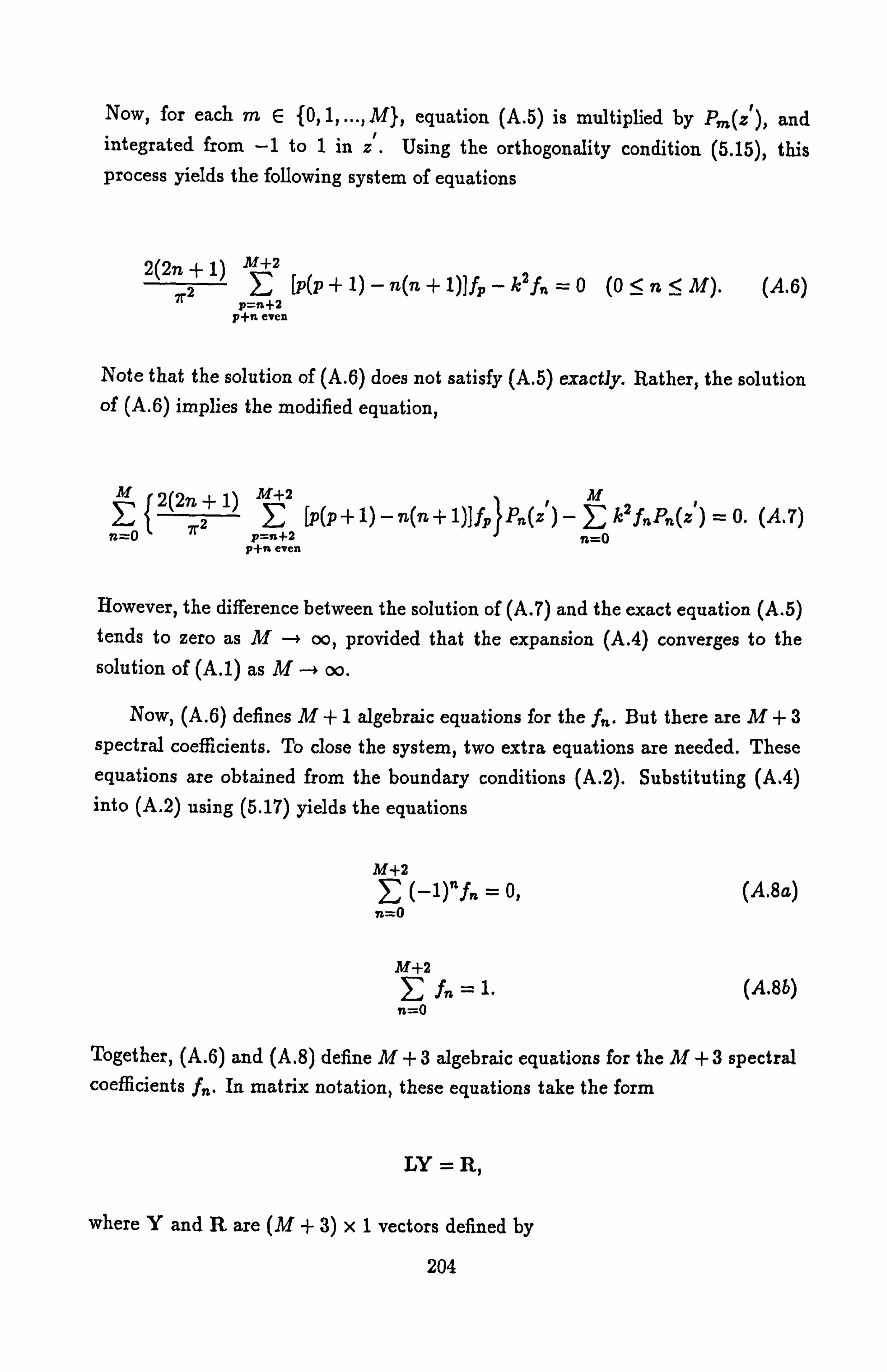
Now, for each mE {O, 1, ..., M}, equation (A. 5) is multiplied by Pm(z'), and integrated from -1 to 1 in z'. Using the orthogonality condition (5.15), this process yields the following system of equations
2(2n + 1) M+2 Z
ý2 [p(p + 1) - n(n + 1)] fp _ A; f� =0 (0 <n< M). (A. 6)
p=n+a p+n even
Note that the solution of (A. 6) does not satisfy (A. 5) exactly. Rather, the solution of (A. 6) implies the modified equation,
ME {2(2n+ 1) 12 [p(p+ 1) - n(n+ 1)]f}P(z') -) k2 fP(z') = 0. (A. ) p=n+2 n_0
p+n even
However, the difference between the solution of (A. 7) and the exact equation (A. 5) tends to zero as M -º oo, provided that the expansion (A. 4) converges to the
solution of (A. 1) as M -+ oo.
Now, (A. 6) defines M+1 algebraic equations for the f,,. But there are M+3
spectral coefficients. To close the system, two extra equations are needed. These
equations are obtained from the boundary conditions (A. 2). Substituting (A. 4) into (A. 2) using (5.17) yields the equations
M+2 E (-1)"f. = 0, (A. 8a) n=O
M+2 In = 1. (A. 8b)
n=0
Together, (A. 6) and (A. 8) define M+3 algebraic equations for the M+3 spectral coefficients f,,. In matrix notation, these equations take the form
LY = R,
where Y and R are (M + 3) x1 vectors defined by
204

yT = {fo
fl f2 .... ,
fM+21
RT = [0
00... 0 1] ,
and L is an (M + 3) x (M + 3) matrix of the form
-k2 0 x 0
o -k2 0 x 0 o -k2 0 x 0 0 0 _k2 L= ,
1 -1 1 -1 1 .. (-1)M+z
1 1 1 1 1 .. 1
where x denotes a nonzero entry. This matrix equation may be set up numeri- cally and solved using NAG routine F04ADF at given values of M. To ensure convergence, it is necessary to check that
If (Z) M+2
-E fnPn(z )I -. 0 as M -+ oo, n=O
for each zE [0,7r], where f is given by (A. 3). In the case where the exact analytic form of f (z) is not known, the test for convergence is slightly different. In such a case (as is considered in the work), define
M-f2 fm(z) _> fPP(z ).
n=0
Then, the method converges if
fM+1(z)-fM(z)l -º0 as M-4oo.
A sequence of functions satisfying this criterion is said to Cauchy, and it can be
shown that a Cauchy sequence converges in the usual sense (see any textbook on
205

analysis). Note that the Tau method can be easily adapted to deal with systems
of equations with multiple boundary conditions.
206
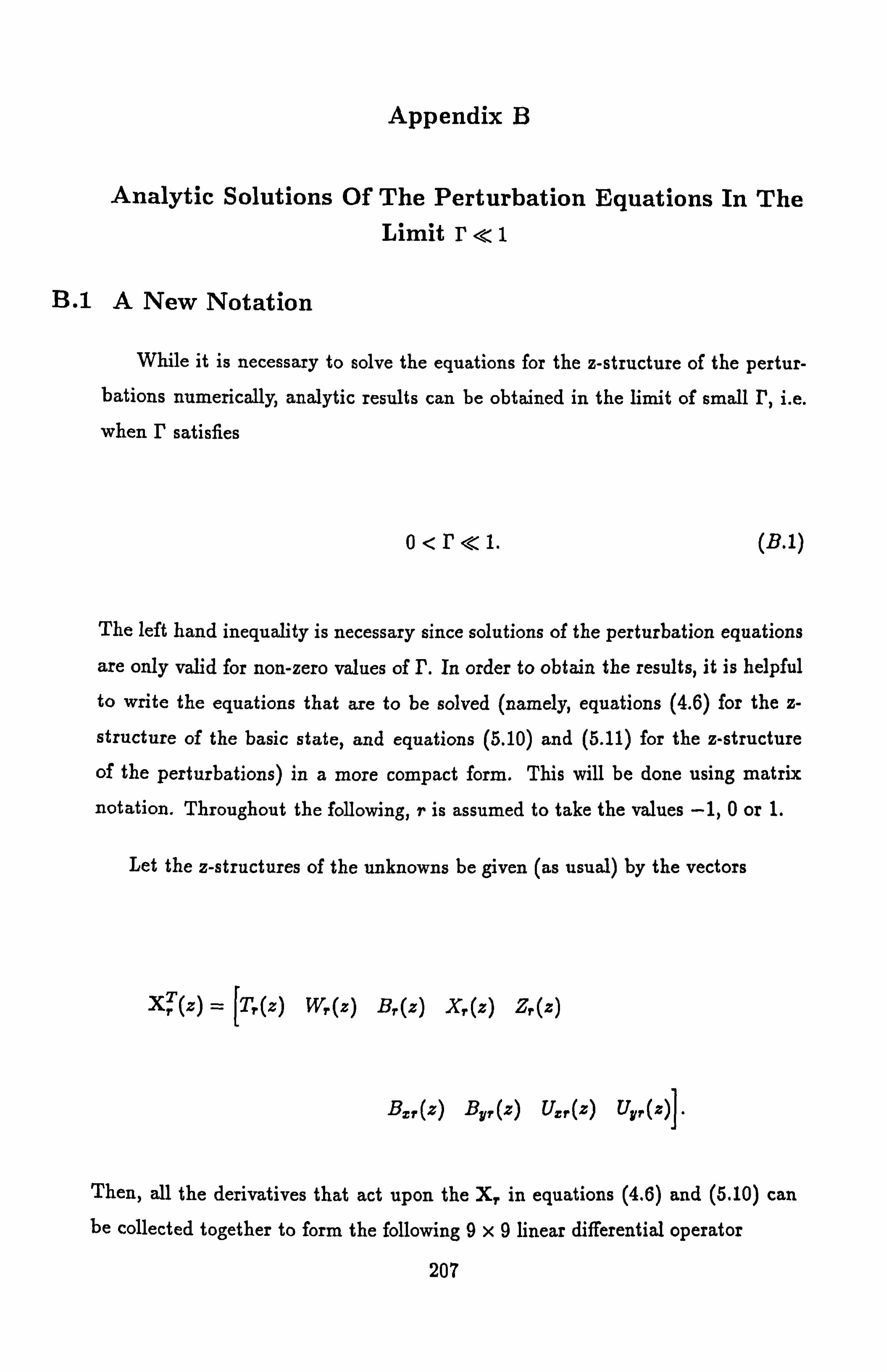
Appendix B
Analytic Solutions Of The Perturbation Equations In The Limit r<1
B. 1 A New Notation
While it is necessary to solve the equations for the z-structure of the pertur- bations numerically, analytic results can be obtained in the limit of small r, i. e.
when r satisfies
o<r«i. (B. 1)
The left hand inequality is necessary since solutions of the perturbation equations
are only valid for non-zero values of r. In order to obtain the results, it is helpful
to write the equations that are to be solved (namely, equations (4.6) for the z-
structure of the basic state, and equations (5.10) and (5.11) for the z-structure
of the perturbations) in a more compact form. This will be done using matrix
notation. Throughout the following, r is assumed to take the values -1,0 or 1.
Let the z-structures of the unknowns be given (as usual) by the vectors
XT '(z) = {T(z) W, -(z) B, (z) X, (z) Z, (z)
B,, (z) By, (z) Uz, (z) Uyr(z)}.
Then, all the derivatives that act upon the Xr in equations (4.6) and (5.10) can be collected together to form the following 9x9 linear differential operator
207
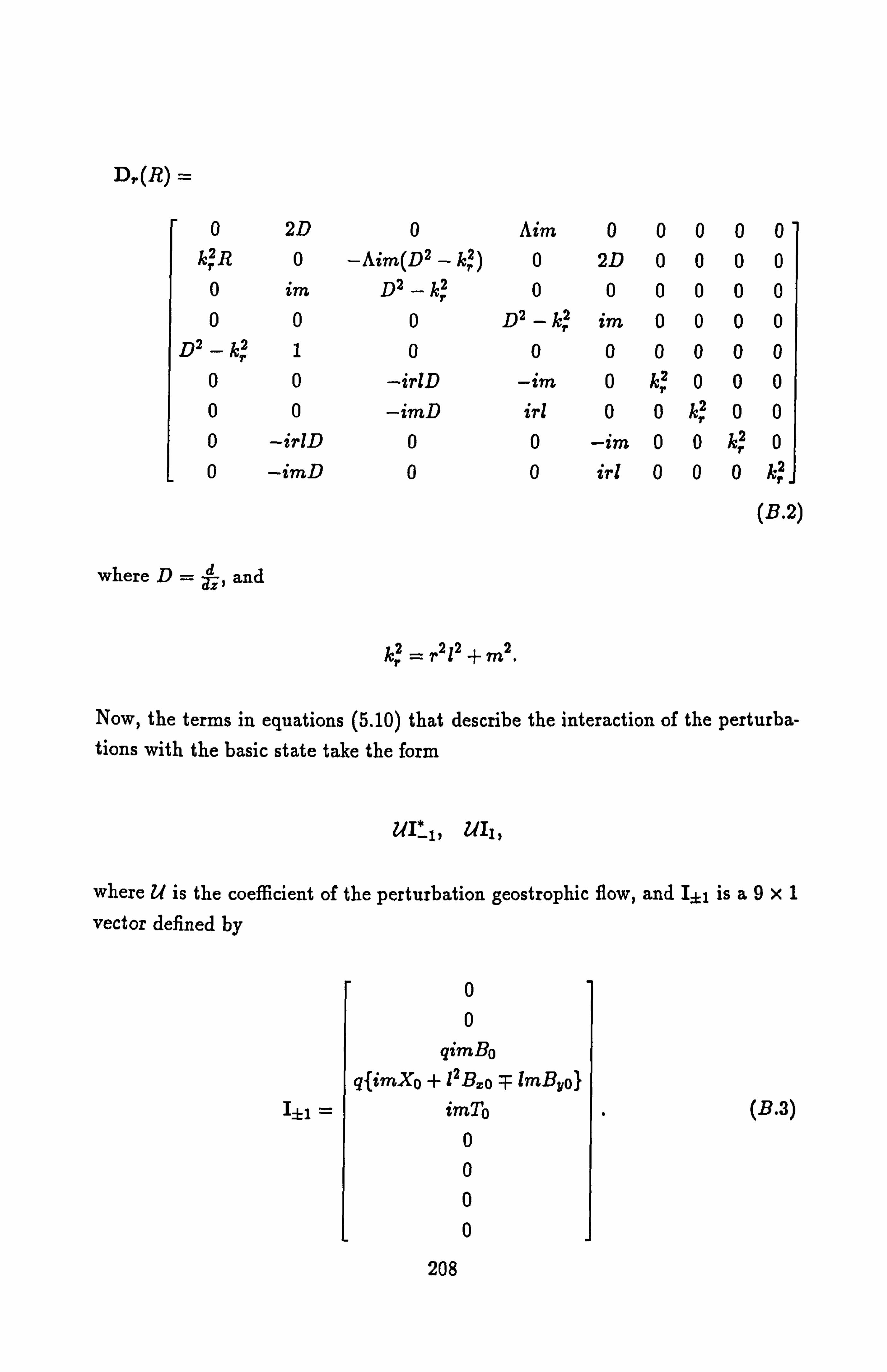
D, (R) =
0 2D 0 Aim 0 0 0 0 0 kTR 0 -Aim(D2 - k? ) 0 2D 0 0 0 0
0 im D2 - kr 0 0 0 0 0 0 0 0 0 DZ - kT im 0 0 0 0
D2-kT 1 0 0 0 0 0 0 0 0 0 -ir1D -im 0 kT 0 0 0 0 0 -imD irl 0 0 k, z 0 0
0 -ir1D 0 0 -im 0 0 kT 0 0 -imD 0 0 irl 0 0 0 k,
(B. 2)
where D= adz-, and
kf = r212 + m2.
Now, the terms in equations (5.10) that describe the interaction of the perturba- tions with the basic state take the form
ui* ,, UIl,
where U is the coefficient of the perturbation geostrophic flow, and I fl is a9x1 vector defined by
I±1 =
0 0
gimBo
q{imXo + 12Bxo lmByo}
imTo
0 0 0 0
(B. 3)
208

Similarly, the terms of (5.10) that involve the complex number
A= 3 -}- 2w,
(where s is the growth rate and w is the frequency of the perturbations) take the form
AJX±i,
where J is a9x9 matrix defined by
J=
000000000 000000000 00g000000
000g00000
100000000 000000000 000000000 000000000 000000000
I. (B. 4)
From these definitions, the equations for the z-structures of the unknowns can be
written in the form
Do(R)Xo = 0, (B. Sa)
{D*_1(Rj - AJ}X_i = L! I*_1, (B. 5b)
{D1(R) - AJJX1 = Lill, (B. 5b)
where U is determined from the equation
209

u= rZ27rn j (BxoByl + BxoBY, -i + Bx, -1Byo + Bx1Byo)dz. (B. 6)
The matrix equation equation (B. 5a) represents equations (4.6) for the z-structure of the basic state (which is given by Xo, as in chapter 4), while (13.5b) and (B. 5c)
represent the equations for the z-structure of the perturbations (which are given by X±I, as in chapter 5). Equation (B. 6) is for the coefficient of the perturbation geostrophic flow, Vi,. These equations are to be solved subject to the boundary
conditions
Wo=Bo=DXo=7b=0 on z=0, (B. 7a)
Wo=Bo -2 =DXo=To-2=0 on z=a, (B. 7b) 4
W_1 = B_1 = DX_i = T_1 =0 on z=0, (B. 7c)
W-1 +i =B_i=DX_1=T_r=0 on z=a, (B. 7d)
W1=B1=DX1=T1=0 on z=0, (B. 7e)
W, -Zmu=B1=DX1=Ti=0 on z=ir. (B. 7f)
As usual, the stability of the basic state to the perturbations is decided by the
sign of s. If s is negative, then the basic state is stable to the perturbations, but
if s is positive, then the basic state is unstable to the perturbations. The critical Rayleigh number, at which the basic state loses stability to the perturbations, is
defined to be that value R,, of R for which
s(Rc) = 0.
210

The value of w at R., denoted by wc ., says how the basic state loses stability. If w, is zero, then the basic state loses stability through the exchange of stabilities; but,
if we is non-zero, then the basic state loses stability through overstability. To find
R, and w,, 3 is set to zero in (B. 5). This yields the following equations
Do(R, )Xo = 0, (B. 8a)
ID*-, (R, ) - iwýJ}X_1 = UI-1i (B. 8b)
iwJ}Xi = Uli, (B. 8c)
7F Z! Ia2ý J(ByoByi +BoBy, _i +Bx, -iByo +Bx1Byo)dz. (B. 8d)
Equations (B. 8) must be solved subject to (B. 7) to obtain Xo, X_1i XI and w, at R=R,.
B. 2 The Method Of Solution
In the limit being considered, i. e. (B. 1), the fact that
r«1,
can be used to obtain analytic solutions of equations (B. 8). This is done by ex-
panding the unknowns as power series in r. Hence, a solution of (B. 8) is sought
of the form
211

00 X, (z) =nrx, (z), (B. 9a)
n=0
00 u= r"un, (B. 9b)
n=l
00 Rc = `, rnRcn, (B. 9c)
n==O
00
WC =E rnWcn. (B. 9d)
n=O (The expansion for U arises as a consequence of (B. 8d), which says that U is
o(r) at leading order). These expansions are substituted into equations (B. 8)
and boundary conditions (B. 7). Using standard methods for manipulating infinite
series, the following equations for the coefficients of the expansions are obtained
Do(Ro)Xon = Fo. (n = 0,1,2... ), (B. 10a)
{D* 1(Rýo) - iwýoJ}X-ln = ý''-ln (n=0,1,2,... ), (B. 10b)
fDI(R, o)-iw, oJIXI, =Fin (n=0,1,2,... ), (B. 10c)
n ZZt1Q un+1 = 1:
a I. 29f
I
`BzomByl, n-m + BomBy-l, n-m
m=0
-i-Bx-l, mByO, n-m +BaimBy0, n-m)dz}
(n = 0,1,2, ... ),
(B. 10d)
where the right hand sides of these equations are given by
212

Fpn =E{- Do(Rcm)Xo, n.. mj(1- öpn), (B. 11a)
{Umti, n_n - {D_i(Rcm) - iwcmJIX_l, n_m}(1 - 60n), (B. 11b)
m=1
F1 _f {UmIi,
n_. m - {D1(Rcm) - iwcmJ}X1, n-m}(1 - boT, ). (B. llc)
m=1
In (B. 11), is the Kronecker delta, D,, (R,, ) is a9x9 matrix defined by
DrýRcný =
000000000 kr Rý, ý 00000000
000000000 000000000 000000000 000000000 000000000 000000000 000000000
and I±1,, ß is a9x1 vector defined by
Ifl, n =
0 0
gimBo�
q{imXon + l2Bxo, lmByon}
imTo.
0 0 0 0
(n=1,2,... ),
to=0,1,2,... ).
(B. 12)
(B. 13)
213

The boundary conditions (B. 7) are satisfied by (B. 9) provided that
W0, ß=Bon=DXo�= Ton=0 on z=0 (n=0,1,2,... ), (ß. 14a)
im Z Won = Boy, - 2q On = DXo,, = Ton. - 2bon, =0 on z= 7r (n = 0,1,2,... ),
(B. 14b)
W -in = B-1n = DX_ln = T-1n =0 on z=0 (n. = 0,1,2,... ), (ß. 14c)
W1+z "(1- So. ) = B-I,, = DX-1,, = T_1, ß =0 on z= 7r (n = 0,1,2,... ), 2
(B. 14d)
W1, = B1n = DX1n = T1n =0 on z=0 (n=0,1,2,... ), (B. 14e)
Win_ imUn(1 -Son) = Bin = DXin = Tin =0 on z= 7r (n = 0,1,2, ...
). (B. 14 f)
Equations (B. 10), (B. 11) and (B. 14) define a hierarchy of problems for the coeffi- cients of the expansions (B. 9), each of which may be solved successively, starting with the n=0 problem. Examination of the equations reveals that Rcn and wcn appear in the equations for the X7, ß. These two quantities are determined to en- sure that the nth system of equations can be solved. This is done by applying solvability conditions to the relevant equations. These solvability conditions will be described later.
214

B. 3 The n=O Problem
The first problem to be considered is the n=0 problem. This is the easiest problem to solve, since there is no coefficient of U to determine at this order. Hence, setting n=0 in equations (B. 10), (B. 11) and (B. 14), the following equa- tions for the 0(1) terms of the expansions (B. 9) are obtained
Do(R, o)Xoo = 0, (B. 15a)
{D1(R0) - iwoJ}X-io = 0, (B. 15b)
{D1(Rýo) - iwoJ}Xio = 0. (B. 15c)
These are to be solved subject to
Woo=Boo=DXoo =Too=0 on z=0, (B. 16a)
Woo=Boo-2 =DXoo=Too-2=0 on z=a, (B. 16b) 9
W io = B-io = DX-io =T io =0 on z=0, (B. 16c)
W io = B-io = DX-io =T 1o =0 on z= ir, (B. 16d)
Wio = Bio = DXjo = T1o =0 on z=0, (B. 16e)
W1o = Bio = DXxo = Tlo =0 on z= ir. (B. 16 f)
Now, the equations and boundary conditions for X_10 and Xlo are identical to those solved in chapter 3 for the Roberts and Stewartson (-) and (+) oblique
215

convection rolls in a standard plane layer. Therefore, the solution of (B. 15b, c) subject to the relevant boundary conditions is given by
X-io(z) = A_IOX-1RS(z), Xjo(z) = AIOXlRS(x), (B. 17)
where X_1RS is defined by (3.49) and XiRS is defined by (3.15). A_lo and A10 are arbitrary complex constants. This solution only exists provided that the following
relation holds
4(giwco+1+k2)2(iwýo+1+k2)+A2m4(iwco+1+k2)(1+k2)
-k2Am2(9iwco +1+ k2)Rco = 0, (B. 18)
where
k2=ki=k? 1=12-+2.
In the context considered here, (B. 18) provides a solvability condition which yields those values of Rco and w, o for which (B. 15) and (B. 16) have a solution. Recall from chapter 3 that (B. 18) has two possible solutions for oblique rolls. Either
wö=U, (B. 19d)
Rco _ 4(1-x- k2)2
+ Am2(1 + k2) (B. 196)
Am2k2 k2
or
2_ (q -1)A2m4(1 + k2) - 4(q + 1)2(1 + k2)2 w co co - 4g2(1 + q)2
_2 4(1 + q)(1 + k2)2 Am2(1 + k2)1 B. 206 ße0
q Am k2 + k2(1 + q) J"()
These are the only values of Rio and woo for which the n=0 problem has a solution.
216

Using the values of R, o in (B. 15a), Xoo can be found exactly as in chapter 4. It is given by
Too(z)
Woo(z)
Boo(z)
Xoo(z)
Xoo(z) = Zoo(z) =
Bx00(z)
Byoo(z)
U oo(z)
Uyoo(Z)
E6=1 ELL Aoon exP(Anz)
r, n_1 (m2 -) )Aoon exP(A Z)
[ten-1 imAoon exp(. 1,
az) + 29
nl mý sinh(mz)
A En_I A-(m2 - an)Aoon eXP(Anz)
ým E6=1 A"(m2 -. 1n)2Aoo,, exp(\nz)
En _1 An(m2 - aý)AOOnexp(Xnz) Amw
- Eý=1 X nAUOn exP('\nz) + 2q sin
1 ma cosh(mz)
21 En=z. n(m2 - ))2A00 eXP(ýnx)
; `-i E=li )n(m2 - .\
)Ao0n exp()tnz)
I
(13.21)
where the . 1,,, are the zeros of the polynomial (4.9) at the point R= Rco, and the Am. are the solutions of the linear equations (4.10). The values of Rco in (4.9)
are given by (B. 19b) or (B. 20b), depending on which case is being considered. Both cases can be considered simultaneously by retaining the term involving woo throughout the calculation.
B. 4 The n=1 Problem
Having solved the n=0 problem, the next step is to solve the n=1 problem for the O(17) terms in the expansions (B. 9). It is at this order that the first effects of the perturbation geostrophic flow are felt. The equations to be solved at this
order are
217
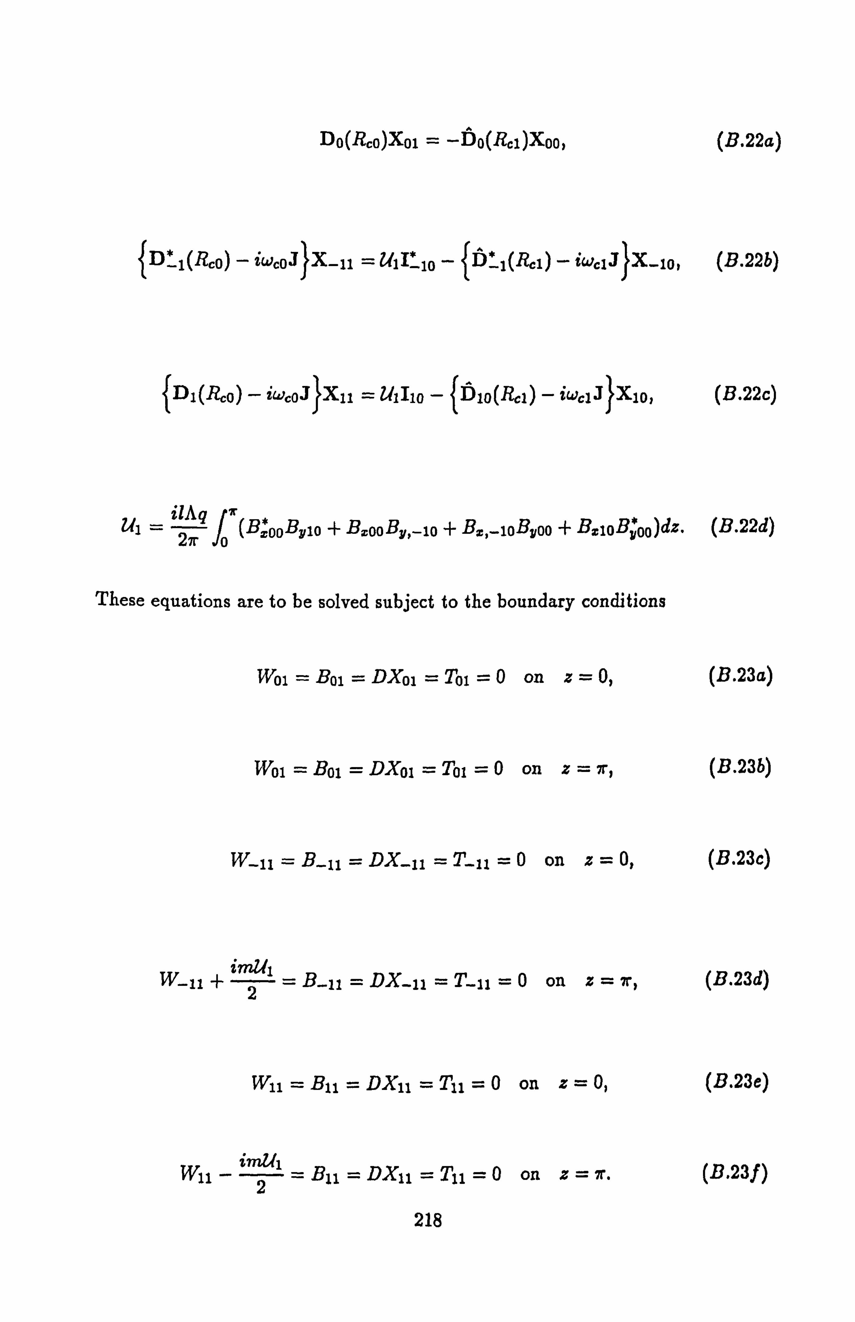
Do(Rco)Xoi = -Do(R, i)Xoo, (ß. 22a)
fD (Rco) - iwcoJ}X-il = Zf1I*_lo - {i1(i1)
- iwc1J}X-lo, (ß. 22b)
{Di(to) - iwoJjxll = UlIio -
{O10(R1) - iwý1J}Xio, (B. 22c)
Ul = 22Lr4 f"(B., *, DoBylo+BxooBy, -lo+Bz, -loBvoo+BtIOBV*00)dz.
(ß. 22d)
These equations are to be solved subject to the boundary conditions
Woi = Boi = DXoi = Toi =0 on z=0, (B. 23a)
Wol = Bol = DXol = T01 =0 on z= 7r, (B. 23b)
W_11 = B_11 = DX-11 = T_11 =0 on z=0, (ß. 23c)
W-11 + zmUi = B_11 = DX-11 = T_11 =0 on z=r, (B. 23d)
Wii = Bii = DX11 = Tii =0 on z=0, (B. 23e)
Wll i mm, = B11 = DXII = Tii =0 on z= ir. (B. 23 f )
2
218

Now, all the quantities on the right hand side of (B. 22d) are known, having
been found in the previous section. It is therefore easy to perform the relevant integrations to find U1. It transpires that
Ui = a1Alo + a2A-lo, (B. 24)
where A10 and A_io are the arbitrary complex constants that arose in the solution
of the n=0 problem, and the an are complex constants, defined by
Aqd -m2 21 1Z al = 2m
I k2(1 + k2 + igwco) + Ak2m 1(1-ý
k+ iwco)I2
Aql -lm 2 j(1 2+ iw°)l�' (B. 25a) 2m
f k2(1 + k2 + igwco) Akz +k
a2 - -Aql f -m2
_ 21 (1 + k2 -I- iwý0)12
2m t k2(1 + k2 + igw, o) Ak2m J
tl l! Im 2 l(1 + k2 + iwco)ii, (B. 25b) _2m lk2(1+k2+igwýo) - AkzJ
where
f DBoo cos(z)dz, (D. 26a) it o
12 a-- Xoo cos(z)dz. (ß. 26b) it
fo
Two problems now arise. The first is that Rol and wcl must be known a priori before equations (B. 24a), (B. 24b) and (B. 24c) can be solved. The second problem
relates to the operators defined by
219

G-i = D* 1(Rýo) - iwoJ, (ß. 27a)
, Cl = D1(Rýo) - iwco]. (B. 27b)
The normal method used to solve the equations
jC-iX-ii = UII_10 - {n1(R1)
- iw,: iJ}X-io) (B. 28a)
Gixii = uiIio - {I510(Ri)
- iwiJ}xio, (ß. 28b)
subject to
W-11 = B_11 = DX-11 = T-11 =0 on z=0, (B. 29a)
W-11 +Zmul=B-11=DX-ii=T_11=0 on z=r, (B. 29b)
W11 = BI1 = DXli = T11 =0 on z=0, (ß. 29c)
Wil zi Bll = DXI1 = T11 =0 on z=a, (ß. 29d) 2
is to write the solutions in the form
X_11 (z) = X. 11(z) + Xpl11 (Z),
X11(2) = Xi2 (z) + Xi2 (z),
where XIx are the free solutions, which satisfy the equations
220

£_1Xf 11 = 0, (ß. 30a)
, 01X11 = 0, (B. 30b)
subject to the boundary conditions (B. 29), while X}1 are the particular integrals,
which are chosen to satisfy the inhomogeneous equations
-iX! '11 -Uli* 10 -
{1i1(R1) - iwc1J}X-lot (B. 31a)
G1Xii = LfiIio - {]10(R1)
- iwc1Jl 10* (B. 31b)
However, because Rio and woo obey the solvability condition (B. 18), solutions of the equations (B. 30) will only obey homogeneous boundary conditions - that is, R, o and wco are the eigenvalues of the operators G±I at which homogeneous solutions
exist. Therefore, (B. 30) cannot be solved subject to (B. 29), since the boundary
conditions (B. 29) are inhomogeneous. Thus, a solution of (B. 28) will only exist
provided that the particular integrals X±11 satisfy the boundary conditions (B. 29)
as well as satisfying (B. 31).
Both problems would be eliminated if Rol and w, could be chosen in such a
way that XP'11 obeyed (B. 29) as well as satisfying (B. 31). The conditions that
ensure that this occurs are called the solvability conditions. To find them, the
adjoint problem to (B. 30) must be considered. Henceforth, X±11 shall be written for X1.
B. 4.1 The Adjoint Problems
Consider the following homogeneous problem. Solve the equations
£1X11 = {Di(Ro)
- iwcoJ}Xu = 0, (8.32)
subject to the boundary conditions
W11=B11=DX11=Ti1=0 on z=0 and z=ir. (B. 33)
221

Define the adjoint vector Xi by
X,, (z) = [Ti(z) Wi (z) Bi (z) Xii(z) Z i(z)
B11(z) B1 1(z) y U 11(z) U ll(z),
> ( B. 34)
and an inner product < .,. > by
a < Y, Z >= -fY. Zdz.
7- o
Now, the inner product of (B. 32) with Xi yields the equation
< Xii, LiXii >= 0.
Evaluating this inner product, and using the formulae
11r 1W -J yDxdz =- [xyJ --f xDydz, is
Jr ir o ir o
I Jr yD2xdz =1
[yDx - xDy]7r +1J zD2ydz,
it o 7r 0 7- o
the following condition (which is equivalent to (B. 36)) is obtained
0 =<, Ci Xii>Xii >+
(B. 35)
(B. 36)
i [Wil(TAl + Uy1 + Ux 1) - Bll(DW11 + DBi1 - Bml - ByI
T
-Til(DZii) - Xii(DXli) + Wii(Zii + DB11) + Bi(DDui)
-Xil(DX1i)+Zi(DTli)]Ol (B. 37) 0
222

where
(D2 - A; 2 - iw"o)ZiI + k2RýoWii
-2DTi1 + imBll + Zli + i1DU411 + imDUU 1
(D2 - k2){B11 - AimWi} - igwcoBli + i1DB il + imDBy11
(D2 - k2 - igw, o)X11 + AimT i- imB. 1+ ilB"
, C`4XA - 1 11 - -2DW i+ imXji - imUU 1+ iZUy 1
kZBxil
k2BYii
k2UZA
k2UA q1I
Using the boundary conditions (B. 33), the condition (B. 37) becomes
10 =< , C1 X1i, Xll >+
lv
[Wi1(Z11 + DB11)
(B. 38)
+Bii(DB411 )- DXii(Xii) + Z41(DTi1)ýý" (B. 39) 10,
Equation (B. 39) is satisfied provided that Xi is chosen to be the solution of
AAB. 40 '1 11 1
subject to the boundary conditions
W11=BA=DXi=Zi=0 on z=0 and z=7r. (B. 41)
223

(B. 40) and (B. 41) define the adjoint problem to (B. 32) and (B. 33). To define the
solvability conditions, only a particular solution of the adjoint problem is required. One such solution is given by
TA (z)
W(z)
Bi (z)
Xi (z)
XA(z) = Zi (z)
Bi1(x)
Bl 1(z)
Uz 1(z)
U411(z)
-21+k2+igoýo Cos(x) Am
sin(z)
Aim 1+k2 sin(z) 1+k +igwco
m` cos(z)
41 Fk2+i wco + Ami 1+k2 1 sin(z) Am 1+k +igwco J
0
0
0
0
This solution exists provided that the following relation holds
4(qiwco +1+ k2)2(iwco +1+ k2) + Azm4(iwco +1+ k2)(1 + k2)
-k2Am2(4iwco +1+ k2)R, o = 0,
(B. 42)
which is precisely the relation defining Rio and wco. This merely says that the
eigenvalues of ACA are the same as those of G1.
In a similar manner, the adjoint problem for the homogeneous equations
c-iX-ii = {D* (Ro) - iwý, oJ}X-ii = 0, (B. 43)
with boundary conditions
224

W_11 = B_11 = DX_11 = T_11 =0 on z=0 and z=w, (B. 44)
can be set up. The details are ommitted, but the following particular solution of the resulting adjoint problem is found
Ti 1(z)
Wit(z)
BA11 (z)
XA11(z)
XA11(z)= ZA11(x)
-21+k2+igwco cos(z) Am
sin(z)
-Aim 1+k2 sin(z) 1+k +iqw o
m cos(z)
J41 hk2+i w, o + Ami 1+k2 J) sin(z)
I. Am 1+k +iq, oo
Bz -ll(z)
By -ii(z)
U4-11(z)
Uv -Ii(z)
0
0
0
0
I. (B. 45)
Again, this solution only exists provided that (B. 18) is satisfied.
The adjoint vectors X11 given by (B. 42) and (B. 45) will now be used to define the solvability conditions for equations (B. 31), which will ensure that the
particular integrals satisfying (B. 31) also obey the boundary conditions (B. 29)
B. 4.2 The Solvability Conditions
Consider now the inhomogeneous equations
{D1(R0) - iw, oJ)X-ii = F-iis (1.46)
225
where
F-11 = U1I*_io - {1Ri)
- iwc1J}X-io. (11.47)
The solution of these equations is required to obey the boundary conditions
W_11 = B_11 = DX_11 = T_11 =0 on z=0, (ß. 48a)
W_11+z 1=B_11=DX_11 =T_11=0 on z=vc. (B. 486)
Form the inner product of (B. 46) with the adjoint vector XA11. This yields the
equation
XAli, C-iX-ii >=< XAi1, F-ii >" (B. 49)
Equation (B. 49) is the required solvability condition for (B. 46).
Using (B. 37), together with the boundary conditions obeyed by XA11 and X_11, the left hand side of (B. 49) yields
XAii, G-iX-i1 >=< GA1XA11, X-ii >+
I [W_11T il + terms that vanish at z=0,7r10'
Now, using the equation satisfied by XA11, i"e.
£AiXA11 = 0,
together with the definition of T 1j in (B. 45), this becomes
21+ k2 + igwco) cos zll <X4>=
[W_ii{ _2(1 Am2
i )J1o'
226

which together with the boundary conditions satisfied by W_11 yields
,q i(1 + k2 + igwco)
X_ii)L_, X-11 >= - aAm U1. (B. 50)
It is a straightforward (but tedious) task to form the inner product of F_11 with XA11. Using the definitions of X±10, and performing the relevant integrations, the
right hand side of (B. 49) yields
_g 2( Z) Is XA, I) F-ii >= {ji2Rci
+ Xiwci}A-io +[1+ k2 + iqwco
2 4(1 + k2 + igwco) Am2(1 + k2)1 l +m2
{k2l2 +lmli
} -im{ Am2 +1+ k2 + z4wco
1 4J Ul'
(B. 51)
where
X_ 2(1+k2+igw, o) +
Am2(1+k2) AmZ 2(1-l- k2 -I- igwo)
_ Am2q(1 + k2)(1-ß k2 + iwco) 2q(1 + k2 + iwCo) (B. 52)
2(1 + k2 + igwco)2 + Am2
and
13 a=-f Boo sin(z)dz, (ß. 53a) ao
1 7r oo sin(z)dz. (13.53b) 14 =-
fo T
Equating (B. 50) and (B. 51), the following equation is obtained
a3Ul - ßA-lo p, (13.54)
where it and a3 are complex constants defined by
227

µ= ýk2Rc1
- Xi",,,
and
(B. 55)
_ -gAm2(1 + k2)I* +
2q {k2l* + IMI* } -imf
4(1 + k2 + igwco) a3 1+k2+igwco 3 m2 2iJ Amt
Am2(1 + k2) 1* i(1 + k2 + igwco) 1+ k2 + igwco J
I4 + irAm
(B. 56)
Now, consider the inhomogeneous equations
, ClXll =
{D1(Ro)
- iw,, oJ}Xii =F il, (B. 57)
where
Fii = u1iro - {I31(n1)
- iweiJIXio" (B. 58)
The solution of these equations is required to obey the boundary conditions
Wil = Bll = DX11 = Tll =0 on z=0, (B. 59a)
Wll -Z1= Bll = DX11 = T11 =0 on z= ir. (B. 59b) 2
To find the solvability condition for (B. 57), the inner product of (D. 57) with Xi is formed. This yields the equation
< Xii,, C1Xli >=< Xli, Fli >. (B. 60)
Repeating the analysis carried out on equation (B. 49), (B. 60) yields the equation
d4U1- µAlo = 0, 228
(B. 61)

where it is given by (B. 55) and a4 is another complex constant defined by
a4= 1+k2+li w2)13+m2{kZIZ-lmll1+im{4(1+ıi4cýco) 9 c0 `
Am2(1 + k2) i(1 + k2 + igwco) 14_ B. 62 1+ k2 -F igwco
I iAm
()
Finally, the solvability conditions for equations (B. 31) take the form
a4U1 - pAlo = 0, (B. 63a)
a3U1 - ILA-10 = 0. (ß. 63b)
Recalling that
Ui = a1Aio + a2A-io,
equations (B. 63) can be written in matrix notation as
CA = µA, (B. 64)
where C is a2x2 complex matrix defined by
ala4 a2a4 (B. 65) C= , alai a2ag
and A is a2x1 complex vector defined by
A . [Aio]. (11.66) A-io
Hence, R. 1 and w, l are obtained from the eigenvalues of C, while Ajo and A-10
are obtained from the eigenvectors of C.
229
The two eigensolutions of (B. 64) are given by
{z=0, A= -a2(B. 67) L al
and
a41 Ii = a2a3 + ala4i A=
a3 J. (B. 68)
Just as in the n=0 case, where two possible values for Rio and woo existed so that
the n=0 equations had a solution, so here two possible values for R1 and wi
exist (obtained from the two possible values of µ) at which the n=1 equations have a solution. These two cases will be discussed seperately.
B. 4.3 The Eigensolution (B. 67)
The first eigensolution is given by (B. 67). Using the definitions of µ and A,
(B. 67) yields
1 k2R� - XZwi = 0, (B. 69a)
[A10 a2 (B. 69b) A-10] _[al
Now, provided that l and m are non zero, then k2 and x are also non zero, whence the real and imaginary parts of (B. 69a) yield
R, 1 = 0, wa = 0,
respectively. Similarly, (B. 69b) yields
Aio = -a2, A-io = al.
(13.70)
(2.71)
These values may be used in equation (B. 24) for Zl1, to obtain
230

U1 = al(-a2) + a2(a1) = 0. (B. 72)
Having obtained Rcl, wcl and U1, equations (B. 22a, b, c) can now be solved. Sub-
stituting (B. 70) and (B. 72) into (B. 22a, b, c) gives
Do(R, o)Xoi = 0, (B. 73a)
{D# 1(R o) - iwoJ}X-ii = 0, (B. 73b)
{DI(Rco) - iwcoJ}Xii = 0, (B. 73c)
while the boundary conditions (B. 23) become
Woi = Boi = DXoi = Toi =0 on z=0 and z=n, (ß. 74a)
W_11=B_11=DX_I1=T_11=0 on z=0 and z=7r, (B. 74b)
W11=B1i=DX11=Tit=0 on z=0 and z=ir. (B. 74c)
A particular integral of (B. 73) and (B. 74) is
Xoi(z) = 0, X_ii (z) ==0, Xll (z) = 0, (B. 75)
and this is the solution of the n=1 equations for this case.
In fact, examination of equations (B. 10) and (B. 11) reveals that by choosing
231
X, n(z) =0 (n = 2,3,... ), (ß. 76a)
14 =0 (n. =2,3,... ), (ß. 76b)
Rcn=0 (n=2,3,... ), (B. 76c)
wc. =0 (n=2,3,... ), (ß. 76d)
an exact, analytic solution of (B. 8) and (B. 7) may be obtained! This analytic
solution is given by
Xo(z) = Xoo(Z), (B. 77a)
X-i(z) = aIX-iRS(z)s (B. 77b)
X, = --a2XlRS(z), (ß. 77c)
u=o, (ß. 77d)
where Xpo is defined by (B. 21), al and a2 are defined by (B. 25), and X±i are the Roberts and Stewartson (±) oblique roll solutions defined in chapter 3. This
solution is discussed further in chapter 5.
13.4.4 The Eigensolution (B. 68)
Attention is now turned to the second eigensolution of (B. 64), which is (8.68).
To compare with the numerics, only the case
A=4,
232

will be considered, for which
Rio=6/, wco=0,12=2- 2,
m2= 2.
At these values, al and a2 are given by (5.46), while a3 and a4 become
a3 = -2V"3qI3 + q(212* + drall) + im(2 - 4ýI4 ), (ß. 78a)
q(2I2 -1mI1) - im(2 - 4-�73-14). (B. 78b) a4 = -2-. /3-gI3
-- 73
Now, because the basic state satisfies the condition (4.21), the integrals IJ must satisfy
=I4. Ii=-II, 12=-12,23=-I3,14
For the parameter values being considered, this fact implies that the a1 satisfy the
conditions
al = -ai, a2 = -az, a3 = -a*, aq = -a4,
and hence, that Ei satisfies
µ- µ*. (8.86)
Therefore, the imaginary part of it vanishes, and so
2ý73-wc1 =0 wcl = 0. (. 1.79)
The real part of µ gives
Rcl = ala4 + a2a3. (B. 80)
233

Using (B. 68) together with the definition of A yields
Alo ja4l = Aio = a4, A-io = a3. (B. 81)
A-io
]=[
a3 J
Using this result in equation (B. 24) for U1 gives
U1 = ala4 + a2a3. (B. 82)
Hence, a second set of values for R, 1, wj and U1 have been found to ensure that the n=1 equations have a solution. These values may be substituted into (B. 24a, b, c) and the relevant particular integral found. Denote the solution of (B. 24a, b, c) with these values of Ri, wi and U1 by
XOi(z), X-10(z), Xio(z).
The actual form taken by the XT1 is very complicated, and is not very enlightening.
234

Bibliography
Abdel-Aziz, M. M. and Jones, C. A., `aw dynamos and Taylor's constraint', Geo-
phys. Astrophys. Fluid Dynamics 44,117-139, (1988).
Barenghi, C. F., `Nonlinear plantary dynamos in a rotating spherical shell II: The
post Taylor equilibrium for a2 dynamos', Geophys. Astrophys. Fluid Dynamics
67,27-36, (1992a).
Barenghi, C. F., `Nonlinear planetary dynamos in a rotating spherical shell III: a2w
models and the geodynamo', Geophys. Astrophys. Fluid Dynamics 71,163-185, (1992b).
Barenghi, C. F. and Jones, C. A., `Nonlinear planetary dynamos in a rotating spheri-
cal shell I: Numerical methods', Geophys. Astrophys. Fluid Dynamics 60,211-243, (1991).
Bell, P. I., `The effect of bumps upon convection in the Earth's core', PhD. disser-
tation, University of Newcastle Upon Tyne, (1993).
Bell, P. I. and Soward, A. M., `The influence of surface topography upon rotating
convection', submitted, (1995).
Bloxham, J. and Gubbins, D., `Thermal core-mantle interactions', Nature 325,
511-513, (1987).
Braginsky, S. I., `Magnetic waves in the Earth's core', Geomag. Aeron. 7,851-859, (1967a).
Braginsky, S. I., `Nearly axially symmetric model of the hydromagnetic dynamo of the Earth I', Geomag. Aeron. 15,122-128, (1975).
Braginsky, S. I., `Nearly axially symmetric model of the hydrodynamic dynamo of the Earth', Geomag. Aeron. 18,225-231, (1978).
Braginsky, S. I., `The z model of the geodynamo with magnetic friction', Geomag. Aeron. 28,407-412, (1988).
235

Busse, F. H., `Thermal instabilities in rapidly rotating systems', J. Fluid Mech. 44, 441-460, (1970).
Busse, F. H. and Wicht, J., `A simple dynamo caused by conductivity variations', Geophys. Astrophys. Fluid Dynamics 64,135-144, (1991).
Chandrasekhar, S., Hydrodynamical and Hydromagnetic Stability, Dover Publica- tions inc., Oxford (1961).
Cowling, T. G., `The magnetic field of sunspots', Mon. Not. R. Astr. Soc. 94, 39-48, (1934).
Eltayeb, I. A. and Kumar, S., `Hydromagnetic convective instbilities of a rotating self-gravitating fluid sphere containing a uniform distribution of heat sources', Proc. R. Soc. Lond. A353,145-162, (1977).
Fearn, D. R., `Thermally driven hydromagnetic convection in a rapidly rotating sphere', Proc. R. Soc. Lond. A369,227-242, (1979a).
Fearn, D. R., `Thermal and magnetic instabilities in a rapidly rotating fluid sphere', Geophys. Astrophys. Fluid Dynamics 14,103-126, (1979b).
Fearn, D. R., `Differential rotation and thermal convection in a rapidly rotating hydromagnetic system', Geophys. Astrophys. Fluid Dynamics 49,173-193, (1989).
Fearn, D. R., 'Nonlinear planetary dynamos' in Stellar and Planetary Dynamos, (eds. M. R. E. Proctor and A. D. Gilbert), Cambridge University Press, (1994).
Fearn, D. R. and Proctor, M. R. E., `Hydromagnetic waves in a differentially rotating sphere', J. Fluid Mech. 128,1-20, (1983a).
Fearn, D. R. and Proctor, M. R. E., `The stabilising role of differential rotation on hrdromagnetic waves', J. Fluid Mech. 128,21-36, (1983b)
Fearn, D. R. and Proctor, M. R. E., `Dynamically consistent magnetic fields pro- duced by differential rotation', J. Fluid Mech. 178,521-534, (1987).
Fearn, D. R. and Proctor, M. R. E., `Magnetogeostrophic balance in non axisym- metric, non-standard dynamo models', Geophys. Astrophys. Fluid Dynamics 67, 117-128, (1992).
Fearn, D. R., Proctor, M. R. E. and Sellar, C. C., `Nonlinear magnetoconvection in
a rotating sphere and Taylor's constraint', Geophys. Astrophys. Fluid Dynamics,
236
77,111-132, (1994).
Fearn, D. R., Roberts, P. H. and Soward, A. M., `Convection, stability and the dy-
namo' in Energy, Stability and Convection, (eds G. P. Galdi and B. Straughan), Pittman Research Notes in Mathematics 168, Longman, (1988).
Greenspan, H. P., The Theory of Rotating Fluids, Cambridge University Press, (1969).
Gottlieb, D. and Orzag, S. A., Numerical Analysis of Spectral Methods, SIAM, (1977).
Gubbins, D. and Richards, M., `Coupling of the core dynamo and mantle: thermal
or topographic? ', Geophys. Res. Lett. 13,1521-1524, (1986).
Gubbins, D. and Bloxham, J., `Morphology of the geomagnetic field and implica-
tions for the geodynamo', Nature 325,509-511, (1987).
Hide, R., `Motions of the Earth's core and mantle and variations of the main
geomagnetic field', Science 157,55-56, (1967).
Hide, R., `Interaction between the Earth's liquid core and solid mantle', Nature
222,1055-1056, (1969).
Hide, R., `Towards a theory of irregular variations in the length of day and core- mantle coupling', Phil. Trans. R. Soc. A284,547-554, (1977).
Hide, R., `Fluctuations in the Earth's rotation and the topography of the core- mantle interface', Phil. Trans. R. Soc. Lond. A328,351-363, (1989).
Hollerbach, R. and Ierley, G. R., `Macrodynamics of a2 dynamos', Geophys. As-
trophys. Fluid Dynamics 56,133-158, (1991).
Hollerbach, R., Barenghi, C. F. and Jones, C. A., `Taylor's constraint in a spherical aw dynamo', Geophys. Astrophys. Fluid Dynamics 67,3-25, (1992).
Ierley, G. R., `Macrodynamics of a2 dynamos', Geophys. Astrophys. Fluid Dy-
namics 34,143-173, (1991).
Geomagnetism II, ed. J. A. Jacobs, London: Academic, (1987).
Jault, D. and Le Moeul, J. -L., `The topographic torque associated with a tangen- tially geostrophic motion at the core surface and inferences on the flow inside the
core', Geophys. Astrophys. Fluid Dynamics 48,273-296, (1989).
237

Jones, C. A., `Dynamo models and Taylor's constraint' in Advances in Solar System MHD (eds. E. R. Priest and A. W. Hood), 25-50, Cambridge University Press, (1991).
Jones, C. A. and Roberts, P. H., `Magnetoconvection in rapidly rotating Boussinesq
and compressible fluids', Geophys. Astrophys. Fluid Dynamics 55,263-308, (1990)
Jones, C. A. and Soward, A. M., `Magnetohydrodynamic dynamo action', Sci. Prog. Oxford 74,529-557, (1990).
Jones, C. A. and Wallace, S. G., `Periodic, chaotic and steady solutions in aw dy-
namos', Geophys. Astrophys. Fluid Dynamics 67,37-64, (1992).
Kelly, R. E. and Pal, D., `Thermal convection with spatially periodic boundary
conditions: resonant wavelength excitation', J. Fluid Mech. 86,433-456, (1977).
Kuang, W. and Bloxham, J., `On the effect of boundary topography on flow in the Earth's core', Geophys. Astrophys. Fluid Dynamics 72,161-195, (1993).
Lanczos, C., Applied Analysis, Prentis-Hall, (1956).
Malkus, W. V. R and Proctor, M. R. E., `The macrodynamics of a-effect dynamos in
rotating fluids', J. Fluid Mech. 67,417-443, (1975).
Moffat, H. K., Magnetic Field Generation in Conducting Fluids, Cambridge Uni-
versity Press, (1978).
Moffat, H. K., `Topographic coupling at the core-mantle interface', Geophys. As-
trophys. Fluid Dynamics 9,279-288, (1978).
Proctor, M. R. E., `Numerical solution of the nonlinear a-effect dynamo equations', J. Fluid Mech. 80,769-784, (1977).
Roberts, P. H., `On the thermal instability of a highly rotating fluid sphere', As-
trophys. J. 141,240-250, (1965).
Roberts, P. H., `On the thermal instability of a rotating fluid sphere containing heat sources', Phil. Trans. R. Soc. Lond. A263,93-117, (1968).
Roberts, P. H., `The future of geodynamo theory', Geophys. Astrophys. Fluid
Dynamics 44,3-31, (1988).
Roberts, P. H., `On topographic core-mantle coupling', Geophys. Asirophys. Fluid Dynamics 44,181-187, (1988).
238

Roberts, P. H., `From Taylor state to model z? ', Geophys. Astrophys. Fluid Dy-
namics 49,143-160, (1989).
Roberts, P. H. and Stewartson, K., `On finite amplitude convection in a rotating magnetic system', Phil. Trans. R. Soc. Lond. A277,93-117, (1974).
Roberts, P. H. and Stewartson, K., `On double roll convection in a rotating mag- netic system', J. Fluid Mech. 68,447-466, (1975).
Rotating Fluids in Geophysics, eds. P. H. Roberts and A. M. Soward, Academic
Press, (1978).
Roberts, P. H. and Soward, A. M., `Dynamo Theory', Annu. Rev. Fluid Mech. 24, 459-512, (1992).
Skinner, P. H. and Soward, A. M., `Convection in a rotating magnetic system and Taylor's constraint', Geophys. Astrophys. Fluid Dynamics 44,91-116, (1988).
Skinner, P. H. and Soward, A. M., `Convection in a rotating magnetic system and Taylor's constraint II: numerical results', Geophys. Astrophys. Fluid Dynamics
60,335-356, (1990).
Soward, A. M., `Thermal and magnetically driven convection in a rapidly rotating fluid layer', J. Fluid Mech. 90,669-684, (1979).
Soward, A. M., `Finite amplitude thermal convection and geostrophic flow in a
rotating magnetic system', J. Fluid Mech. 98,449-471, (1980).
Soward, A. M., `Nonlinear marginal convection in a rotating magnetic system', Geophys. Astrophys. Fluid Dynamics 35,329-371, (1986).
Soward, A. M., `The Earth's dyanamo', Geophys. Astrophys. Fluid Dynamics 62,
191-209, (1991).
Soward, A. M. and Jones, C. A., `a2 dynamos and Taylor's constraint', Geophys. Astrophys. Fluid Dynamics 27,87-122, (1983).
Sun, Z. P., Schubert, G. and Glatzmaier, G. A., `Numerical simulations of ther-
mal convection in a rapidly rotating spherical shell cooled inhomogeneously from
above', Geophys. Astrophys. Fluid Dynamics 75,199-226, (1994).
Taylor, J. B., `The magnetohydrodynamics of a rotating fluid and the Earth's dy-
namo problem', Proc. R. Soc. Lond. A274,274-283, (1963).
239

Voorhies, C. V., `Coupling an inviscid core to an electrically insulating mantle', J. Geomagn. Geoelectr. 43,131-156, (1991).
Zhang, K. K., `Convection in a rapidly rotating spherical shell at infinite Prantl
number: steadily drifting rolls', Phys. Earth Planet. Interiors 68,156-169, (1991).
Zhang, K. K. and Gubbins, D., ` On convection in the Earth's core driven by lateral
temperature variations', Geophys. J. Int. 108,247-255, (1992).
Zhang, K. K. and Gubbins, D., `Convection in a rotating spherical shell with an inhomogeneous temperature boundary at infinite Prantl number', J. Fluid Mech.
250,209-232, (1993).
240


![Natural Convection Flow of Fractional Nanofluids Over an … · 2017-05-07 · Mondal et al. [5] considered the unsteady magneto-hydrodynamic axi-symmetric stagnation-point flow](https://cdn.vdocument.in/doc/165x107/5e749ee3ba90555cd97ef0b9/natural-convection-flow-of-fractional-nanofluids-over-an-2017-05-07-mondal-et.jpg)
