The Kronecker Product
A Product of the Times
Charles Van Loan
Department of Computer Science
Cornell University
Presented at the SIAM Conference on Applied Linear Algebra, Monterey, Califirnia,
October 26, 2009
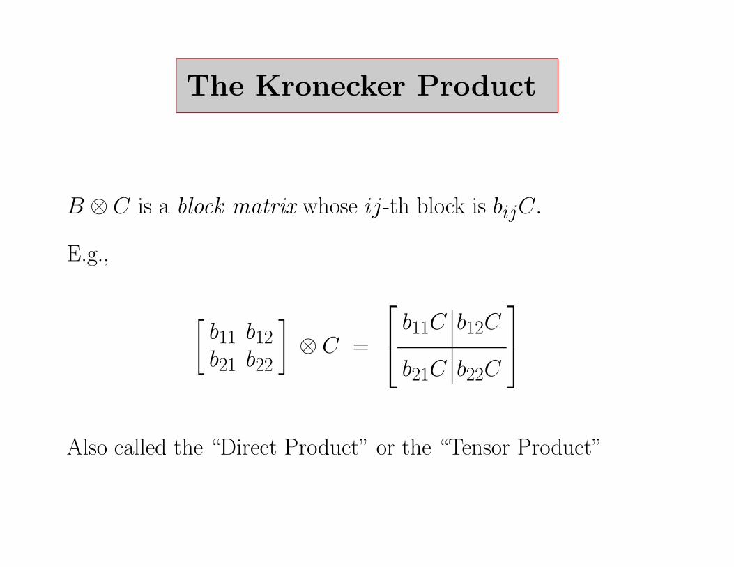
The Kronecker Product
B ⊗ C is a block matrix whose ij-th block is bijC.
E.g.,
[
b11 b12b21 b22
]
⊗ C =
b11C b12C
b21C b22C
Also called the “Direct Product” or the “Tensor Product”
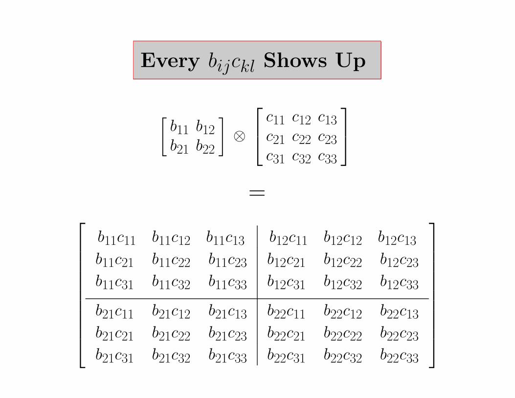
Every bijckl Shows Up
[
b11 b12b21 b22
]
⊗
c11 c12 c13c21 c22 c23c31 c32 c33
=
b11c11 b11c12 b11c13 b12c11 b12c12 b12c13
b11c21 b11c22 b11c23 b12c21 b12c22 b12c23
b11c31 b11c32 b11c33 b12c31 b12c32 b12c33
b21c11 b21c12 b21c13 b22c11 b22c12 b22c13
b21c21 b21c22 b21c23 b22c21 b22c22 b22c23
b21c31 b21c32 b21c33 b22c31 b22c32 b22c33

Basic Algebraic Properties
(B ⊗ C)T = BT ⊗ CT
(B ⊗ C)−1 = B−1 ⊗ C−1
(B ⊗ C)(D ⊗ F ) = BD ⊗ CF
B ⊗ (C ⊗ D) = (B ⊗ C) ⊗ D
C ⊗ B = (Perfect Shuffle)T (B ⊗ C)(Perfect Shuffle)
R.J. Horn and C.R. Johnson(1991). Topics in Matrix Analysis, Cambridge University Press, NY.

Reshaping KP Computations
Suppose B,C ∈ IRn×n and x ∈ IRn2.
The operation y = (B ⊗ C)x is O(n4):
y = kron(B,C)*x
The equivalent, reshaped operation Y = CXBT is O(n3):
y = reshape(C*reshape(x,n,n)*B’,n,n)
H.V. Henderson and S.R.Searle (1981). “The Vec-Permutation Matrix, The Vec Operator,and Kronecker Products, A Review,” Linear and Mulitilinear Algebra, 9, 271–288.

Talk Outline
1. The 1800’s
Origins: ©Z2. The 1900’s
Heightened Profile: ⊗ ⊗ ⊗ ⊗ ⊗ ⊗ ⊗ ⊗ ⊗ ⊗3. The 2000’s
Future: ©∞

The 1800’s
©Z
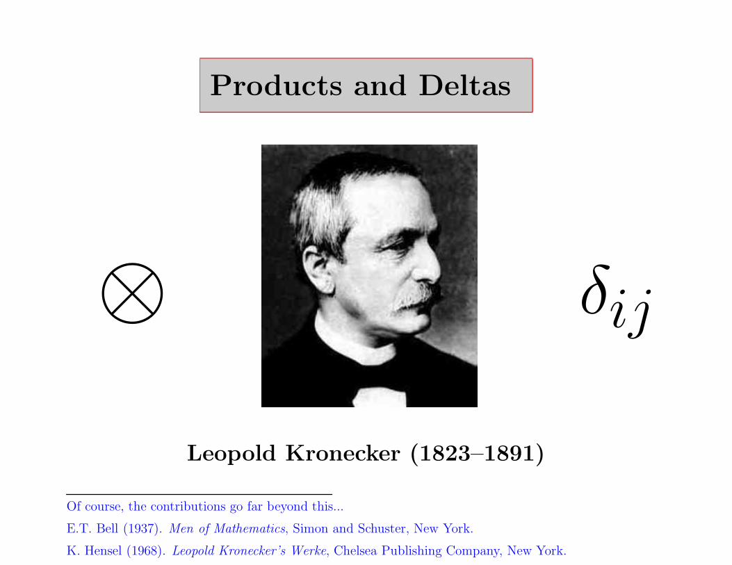
Products and Deltas
⊗ δij
Leopold Kronecker (1823–1891)
Of course, the contributions go far beyond this...
E.T. Bell (1937). Men of Mathematics, Simon and Schuster, New York.
K. Hensel (1968). Leopold Kronecker’s Werke, Chelsea Publishing Company, New York.
Brief Survey of the Kronecker Delta
UT δijV =∣
∣δij
∣
∣
κ2(δij) = 1δij
G.H. Golub and C. Van Loan (1996). Matrix Computations, 3rd Ed., Johns Hopkins University Press,Baltimore, Maryland.
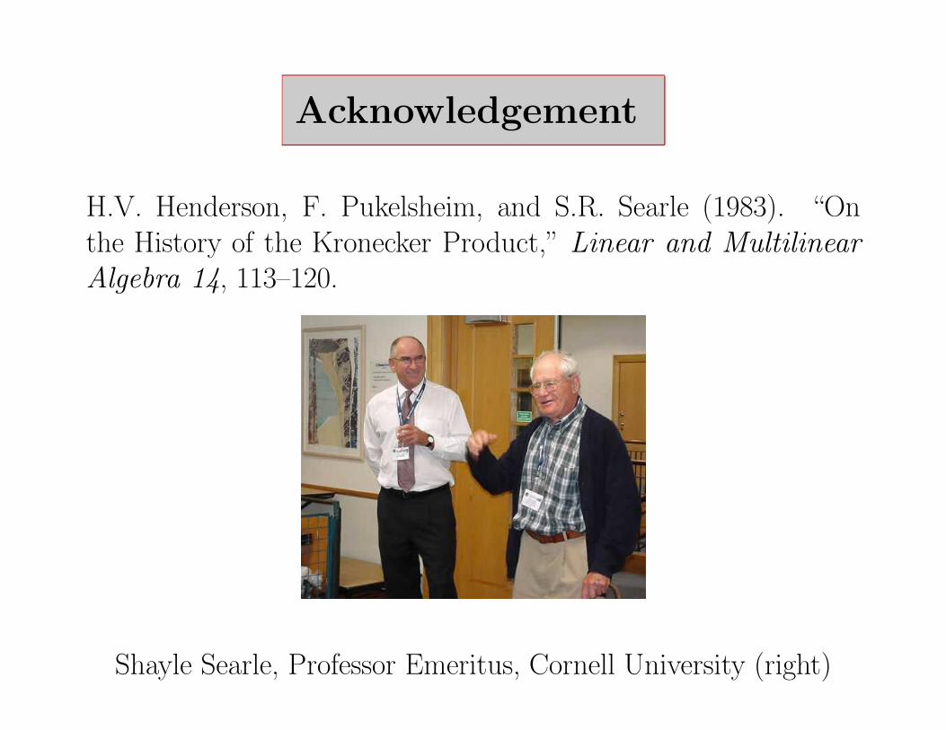
Acknowledgement
H.V. Henderson, F. Pukelsheim, and S.R. Searle (1983). “Onthe History of the Kronecker Product,” Linear and Multilinear
Algebra 14, 113–120.
Shayle Searle, Professor Emeritus, Cornell University (right)

Scandal!
H.V. Henderson, F. Pukelsheim, and S.R. Searle (1983). “Onthe History of the Kronecker Product,” Linear and Multilinear
Algebra 14, 113–120.
Abstract
History reveals that what is today called the Kro-necker product should be called the Zehfuss Product.
This fact is somewhat appreciated by the modern (numerical) linear algebra community:
R.J. Horn and C.R. Johnson(1991). Topics in Matrix Analysis, Cambridge University Press, NY, p. 254.
A.N. Langville and W.J. Stewart (2004). “The Kronecker product and stochastic automata networks,” J.
Computational and Applied Mathematics 167, 429–447.

Who Was Zehfuss?
Born 1832.
Obscure professor of mathematics at University of Heidelberg fora while. Then went on to other things.
Wrote papers on determinants...
G. Zehfuss (1858). “Uber eine gewisse Determinante,” Zeitschrift fur Mathematik undPhysik 3, 298–301.
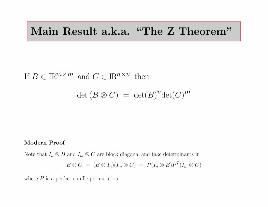
Main Result a.k.a. “The Z Theorem”
If B ∈ IRm×m and C ∈ IRn×n then
det (B ⊗ C) = det(B)ndet(C)m
Modern Proof
Note that In ⊗ B and Im ⊗ C are block diagonal and take determinants in
B ⊗ C = (B ⊗ In)(Im ⊗ C) = P (In ⊗ B)P T (Im ⊗ C)
where P is a perfect shuffle permutation.

Excerpts from Zehfuss(1858)
∆ =
∣
∣
∣
∣
∣
∣
∣
∣
∣
∣
∣
∣
∣
∣
∣
∣
∣
∣
∣
∣
∣
∣
∣
∣
∣
a1A1 a1B1 b1A1 b1B1 c1A1 c1B1 d1A1 d1B1
a1A2 a1B2 b1A2 b1B2 c1A2 c1B2 d1A2 d1B2
a2A1 a2B1 b2A1 b2B1 c2A1 c2B1 d2A1 d2B1
a2A2 a2B2 b2A2 b2B2 c2A2 c2B2 d2A2 d2B2
a3A1 a3B1 b3A1 b3B1 c3A1 c3B1 d3A1 d3B1
a3A2 a3B2 b3A2 b3B2 c3A2 c3B2 d3A2 d3B2
a4A1 a4B1 b4A1 b4B1 c4A1 c4B1 d4A1 d4B1
a4A2 a4B2 b4A2 b4B2 c4A2 c4B2 d4A2 d4B2
∣
∣
∣
∣
∣
∣
∣
∣
∣
∣
∣
∣
∣
∣
∣
∣
∣
∣
∣
∣
∣
∣
∣
∣
∣
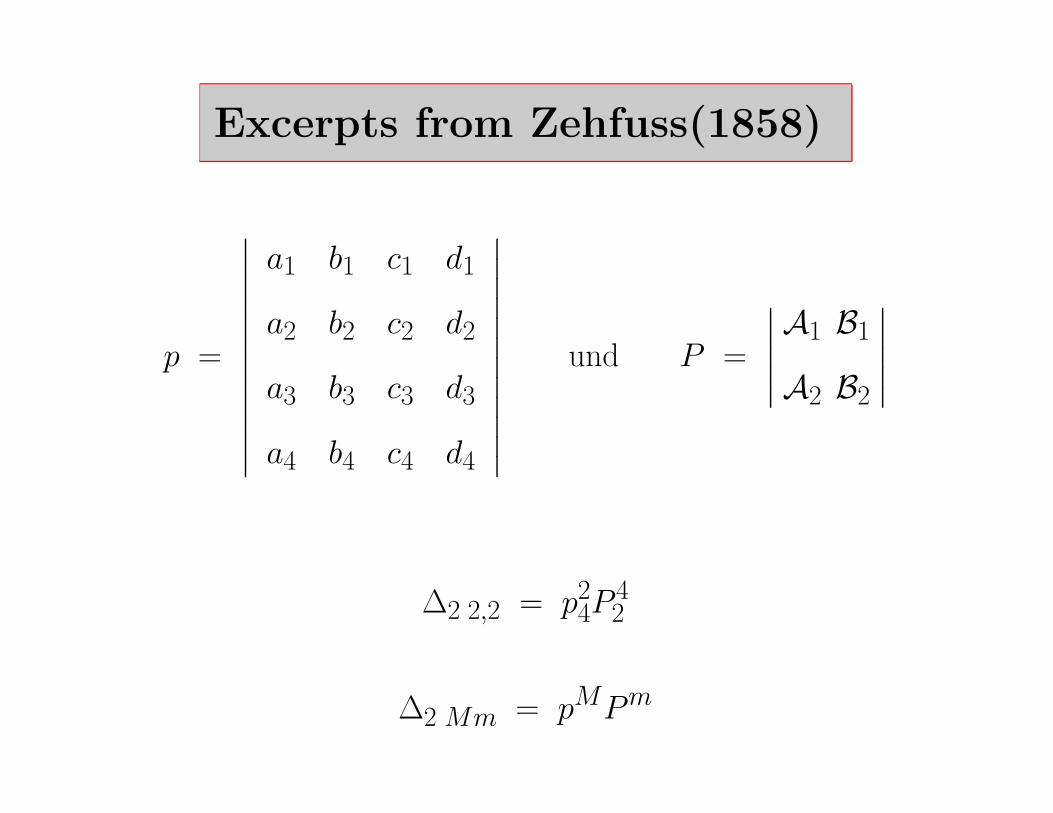
Excerpts from Zehfuss(1858)
p =
∣
∣
∣
∣
∣
∣
∣
∣
∣
∣
∣
∣
a1 b1 c1 d1
a2 b2 c2 d2
a3 b3 c3 d3
a4 b4 c4 d4
∣
∣
∣
∣
∣
∣
∣
∣
∣
∣
∣
∣
und P =
∣
∣
∣
∣
∣
A1 B1
A2 B2
∣
∣
∣
∣
∣
∆2 2,2 = p24P
42
∆2 Mm = pMPm
Hensel (1891)
Student in Berlin 1880-1884.
Maintains that Kronecker presented the Z-theorem in his lectures.
K. Hensel (1891). “Uber die Darstellung der Determinante eines Systems, welches aus zwei anderencomponirt ist,” ACTA Mathematica 14, 317–319.

The 1900’s
⊗ ⊗ ⊗ ⊗ ⊗ ⊗ ⊗ ⊗ ⊗ ⊗

Muir (1911)
Attributes the Z-theorem to Zehfuss.
Calls det(B ⊗ C) the “Zehfuss determinant.”
T. Muir (1911). The Theory of Determinants in the Historical Order of Development, Vols 1-4, Dover,NY.
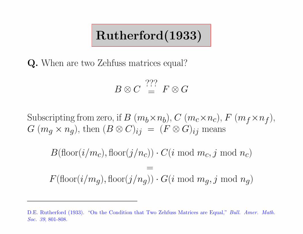
Rutherford(1933)
Q. When are two Zehfuss matrices equal?
B ⊗ C???= F ⊗ G
Subscripting from zero, if B (mb×nb), C (mc×nc), F (mf×nf ),G (mg × ng), then (B ⊗ C)ij = (F ⊗ G)ij means
B(floor(i/mc), floor(j/nc)) · C(i mod mc, j mod nc)
=F (floor(i/mg), floor(j/ng)) · G(i mod mg, j mod ng)
D.E. Rutherford (1933). “On the Condition that Two Zehfuss Matrices are Equal,” Bull. Amer. Math.
Soc. 39, 801-808.

©Z → ⊗ Why?
“...a series of influential texts at and after the turn of thecentury permanently associated Kronecker’s name with the“ ⊗ ” product and this terminology is nearly universal to-day.”
Horn and Johnson (1991)
“...the textbook of Scott and Matthews (1904) which ap-peared four years after the publication of Rados’ paper,gave new life to the old error. This was probably due tothe teaching of Pascal, whose second edition (1923) stillpropagates the error [of the first edition (1897).]”
Muir (1927)
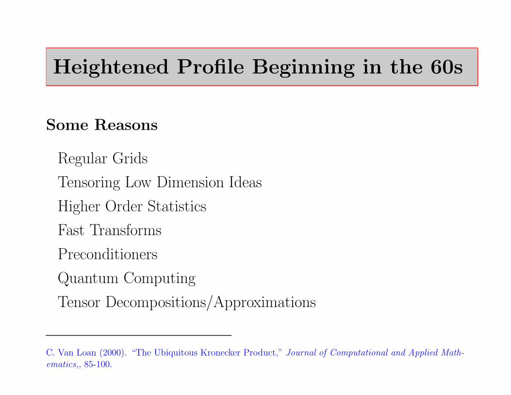
Heightened Profile Beginning in the 60s
Some Reasons
Regular Grids
Tensoring Low Dimension Ideas
Higher Order Statistics
Fast Transforms
Preconditioners
Quantum Computing
Tensor Decompositions/Approximations
C. Van Loan (2000). “The Ubiquitous Kronecker Product,” Journal of Computational and Applied Math-
ematics,, 85-100.

Regular Grids
(M +1)-by-(N +1) discretization of the Laplacian on a rectangle...
A = IM ⊗ TN + TM ⊗ IN
T5 =
2 −1 0 0 0−1 2 −1 0 0
0 −1 2 −1 00 0 −1 2 −10 0 0 −1 2
F.W. Dorr (1970). “The Direct Solution of the Discrete Poisson Equation on a Rectangle,” SIAM Review
12, 248–263.
G.H. Golub and C.F. Van Loan (1996). Matrix Computations, 3rd Ed, Johns Hopkins University Press,
Baltimore, MD.
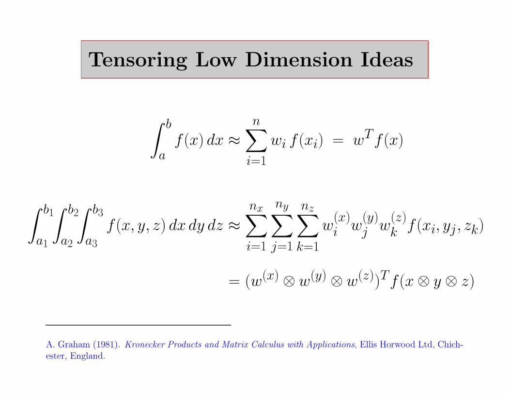
Tensoring Low Dimension Ideas
∫ b
af (x) dx ≈
n∑
i=1
wi f (xi) = wTf (x)
∫ b1
a1
∫ b2
a2
∫ b3
a3
f (x, y, z) dx dy dz ≈nx∑
i=1
ny∑
j=1
nz∑
k=1
w(x)i w
(y)j w
(z)k f (xi, yj, zk)
= (w(x) ⊗ w(y) ⊗ w(z))Tf (x ⊗ y ⊗ z)
A. Graham (1981). Kronecker Products and Matrix Calculus with Applications, Ellis Horwood Ltd, Chich-ester, England.
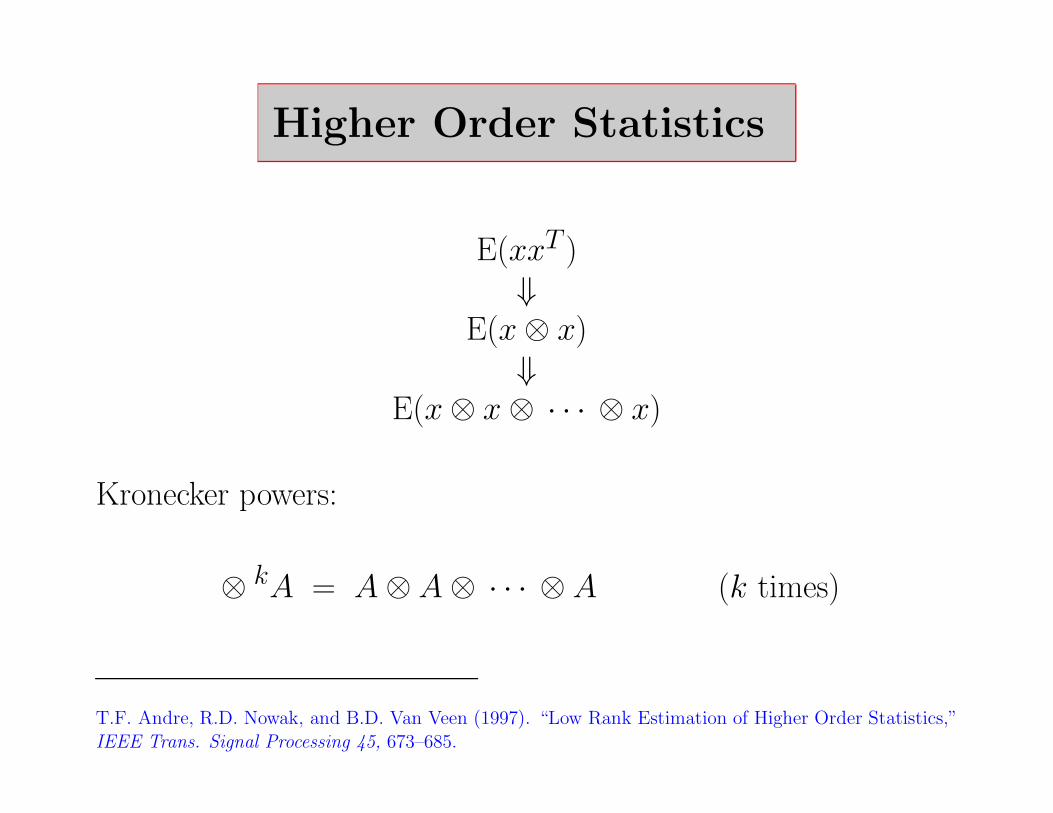
Higher Order Statistics
E(xxT )⇓
E(x ⊗ x)⇓
E(x ⊗ x ⊗ · · · ⊗ x)
Kronecker powers:
⊗ kA = A ⊗ A ⊗ · · · ⊗ A (k times)
T.F. Andre, R.D. Nowak, and B.D. Van Veen (1997). “Low Rank Estimation of Higher Order Statistics,”IEEE Trans. Signal Processing 45, 673–685.

Fast Transforms
FFT
F16P16 = B16(I2 ⊗ B8)(I4 ⊗ B4)(I8 ⊗ B2)
B4 =
1 0 1 00 1 0 ω41 0 −1 00 1 0 −ω4
ωn = exp(−2πi/n)
J. Granata, M. Conner, and R. Tolimieri (1992). “Recursive Fast Algorithms and the Role of the Tensor
Product,” IEEE Transactions on Signal Processing 40, 2921–2930.
C. Van Loan(1992). Computational Frameworks for the Fast Fourier Transform, SIAM Publications,
Philadelphia, PA.
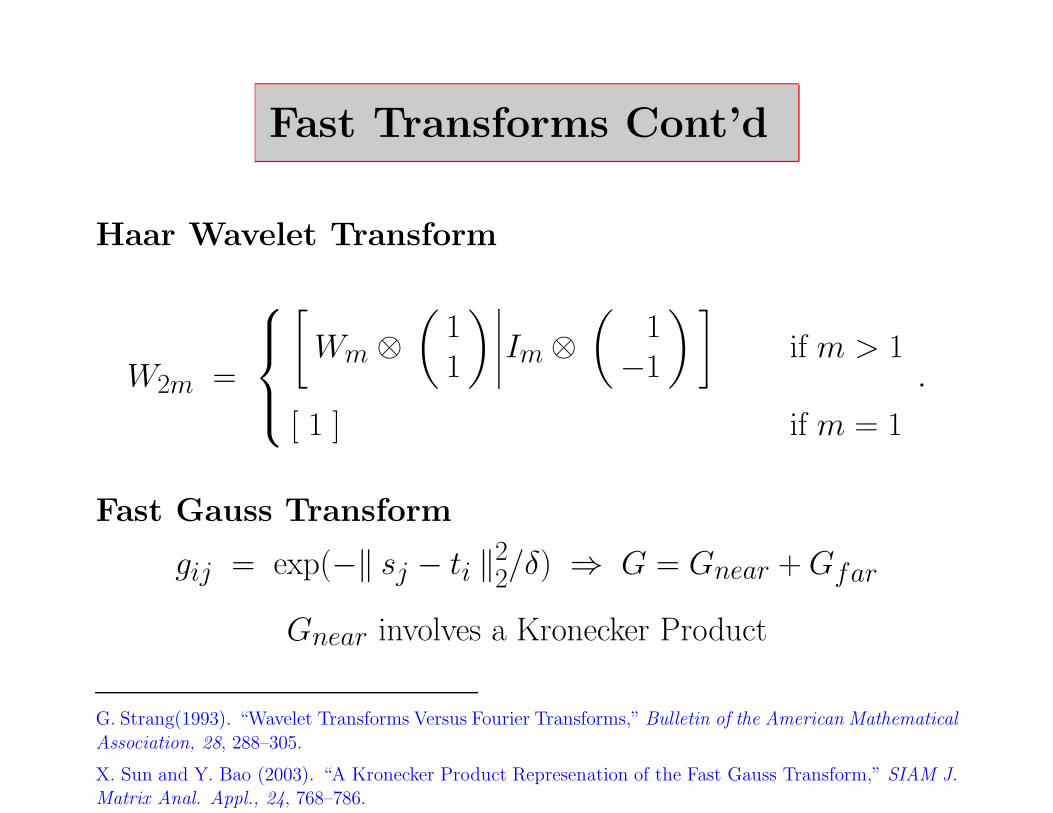
Fast Transforms Cont’d
Haar Wavelet Transform
W2m =
[
Wm ⊗(
11
)
Im ⊗(
1−1
) ]
if m > 1
[ 1 ] if m = 1
.
Fast Gauss Transform
gij = exp(−‖ sj − ti ‖22/δ) ⇒ G = Gnear + Gfar
Gnear involves a Kronecker Product
G. Strang(1993). “Wavelet Transforms Versus Fourier Transforms,” Bulletin of the American Mathematical
Association, 28, 288–305.
X. Sun and Y. Bao (2003). “A Kronecker Product Represenation of the Fast Gauss Transform,” SIAM J.
Matrix Anal. Appl., 24, 768–786.
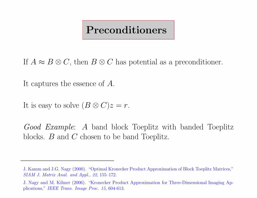
Preconditioners
If A ≈ B ⊗ C, then B ⊗ C has potential as a preconditioner.
It captures the essence of A.
It is easy to solve (B ⊗ C)z = r.
Good Example: A band block Toeplitz with banded Toeplitzblocks. B and C chosen to be band Toeplitz.
J. Kamm and J.G. Nagy (2000). “Optimal Kronecker Product Approximation of Block Toeplitz Matrices,”
SIAM J. Matrix Anal. and Appl., 22, 155–172.
J. Nagy and M. Kilmer (2006). “Kronecker Product Approximation for Three-Dimensional Imaging Ap-plications,” IEEE Trans. Image Proc. 15, 604-613.
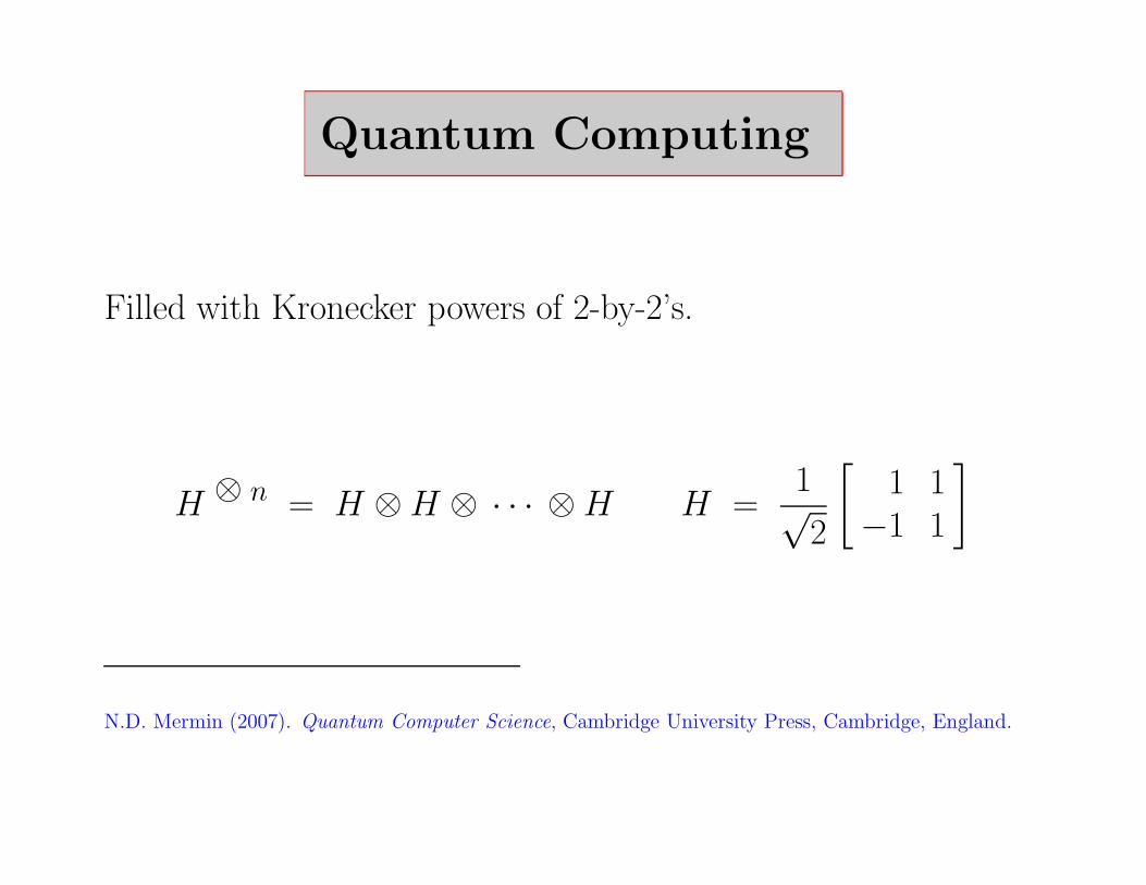
Quantum Computing
Filled with Kronecker powers of 2-by-2’s.
H ⊗ n = H ⊗ H ⊗ · · · ⊗ H H =1√2
[
1 1−1 1
]
N.D. Mermin (2007). Quantum Computer Science, Cambridge University Press, Cambridge, England.

Tensor Decompositions/Approximation
E.g. Given A = A(1:n, 1:n, 1:n, 1:n), find orthogonal
Q =[
q1 · · · qn]
U =[
u1 · · · un]
V =[
v1 · · · vn]
W =[
w1 · · · wn]
and a “core tensor” σ so
vec(A) ≈n
∑
i,j,k,`=1
σijk,` wi ⊗ vj ⊗ uk ⊗ q`
T. Kolda and B. Bader (2009). “Tensor Decompositions and Applications,” SIAM Review 51, 455–500.

Descendants
1. The Left Kronecker Product
2. The Hadamard Product
3. The Tracy-Singh Product
4. The Khatri-Rao Product
5. The Generalized Kronecker Product
6. The Strong Kronecker Product
7. The Symmetric Kronecker Product
8. The Bi-Alternate Product

Left Kronecker Product
Definition:
BLeft⊗
[
c11 c12
c21 c22
]
=
[
c11B c12B
c21B c22B
]
= C ⊗ B
Fact:
If B ∈ IRmb×nb and C ∈ IRmc×nc then
BLeft⊗ C = ΠT
mc, mbmc(B ⊗ C)Πnc, nbnc
↑ Perfect Shuffles ↑
F.A. Graybill(1969). Introduction to Matrices with Applications in Statistics, Wadsworth, Belmont, CA.

The Hadamard Product
Definition:
b11 b12
b21 b22
b31 b32
Had⊗
c11 c12
c21 c22
c31 c32
=
b11c11 b12c12
b21c21 b22c22
b31c31 b32c32
BHad⊗ C = B. ∗ C
A. Smilde, R. Bro, and P. Geladi (2004). Multiway Analysis, John Wiley, Chichester, England.

The Hadamard Product
Fact:
If A = B ⊗ C and B,C ∈ IRm×n , then
BHad⊗ C = A(1:(m+1):m2, 1:(n+1):n2)
E.g.,
b11 b12
b21 b22
b31 b32
⊗
c11 c12
c21 c22
c31 c32
=
b11c11 b11c12 b12c11 b12c12
b11c21 b11c22 b12c21 b12c22
b11c31 b11c32 b12c31 b12c32
b21c11 b21c12 b22c11 b22c12
b21c21 b21c22 b22c21 b22c22
b21c31 b21c32 b22c31 b22c32
b31c11 b31c12 b32c11 b32c12
b31c21 b31c22 b32c21 b32c22
b31c31 b31c32 b32c31 b32c32
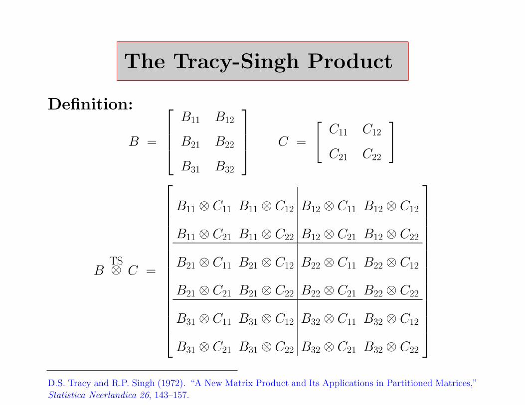
The Tracy-Singh Product
Definition:
B =
B11 B12
B21 B22
B31 B32
C =
[
C11 C12
C21 C22
]
BTS⊗ C =
B11 ⊗ C11 B11 ⊗ C12 B12 ⊗ C11 B12 ⊗ C12
B11 ⊗ C21 B11 ⊗ C22 B12 ⊗ C21 B12 ⊗ C22
B21 ⊗ C11 B21 ⊗ C12 B22 ⊗ C11 B22 ⊗ C12
B21 ⊗ C21 B21 ⊗ C22 B22 ⊗ C21 B22 ⊗ C22
B31 ⊗ C11 B31 ⊗ C12 B32 ⊗ C11 B32 ⊗ C12
B31 ⊗ C21 B31 ⊗ C22 B32 ⊗ C21 B32 ⊗ C22
D.S. Tracy and R.P. Singh (1972). “A New Matrix Product and Its Applications in Partitioned Matrices,”
Statistica Neerlandica 26, 143–157.

The Khatri-Rao Product
Definition:
B =
B11 B12
B21 B22
B31 B32
C =
C11 C12
C21 C22
C31 C32
BK-R⊗ C =
B11 ⊗ C11 B12 ⊗ C12
B21 ⊗ C21 B22 ⊗ C22
B31 ⊗ C31 B32 ⊗ C32
C.R. Rao and S.K. Mitra (1971). Generalized Inverse of Matrices and Applications, John Wiley and Sons,New York.
A. Smilde, R. Bro, and P. Geladi (2004). Multiway Analysis, John Wiley, Chichester, England.

The Khatri-Rao Product
Fact:
BKR⊗ C is a submatrix of B
TS⊗ C
BTS⊗ C =
B11 ⊗ C11 B11 ⊗ C12 B12 ⊗ C11 B12 ⊗ C12
B11 ⊗ C21 B11 ⊗ C22 B12 ⊗ C21 B12 ⊗ C22
B11 ⊗ C31 B11 ⊗ C32 B12 ⊗ C31 B12 ⊗ C32
B21 ⊗ C11 B21 ⊗ C12 B22 ⊗ C11 B22 ⊗ C12
B21 ⊗ C21 B21 ⊗ C22 B22 ⊗ C21 B22 ⊗ C22
B21 ⊗ C31 B21 ⊗ C32 B22 ⊗ C31 B22 ⊗ C32
B31 ⊗ C11 B31 ⊗ C12 B32 ⊗ C11 B32 ⊗ C12
B31 ⊗ C21 B31 ⊗ C22 B32 ⊗ C21 B32 ⊗ C22
B31 ⊗ C31 B31 ⊗ C32 B32 ⊗ C31 B32 ⊗ C32

The Generalized Kronecker Product
B1
B2
B3
B4
gen⊗ C =
B1
Left⊗ C(1, :)
B2
Left⊗ C(2, :)
B3
Left⊗ C(3, :)
B4
Left⊗ C(4, :)]
Regalia and Mitra (1989), “Kronecker Products, Unitary Matrices, and Signal Processing Applications,”SIAM Review, 31, 586–613.

The Generalized Kronecker Product
B1B2B3B4
GEN⊗{
C1C2
}
=
{
B1B2
}
gen⊗ C1
{
B3B4
}
gen⊗ C2
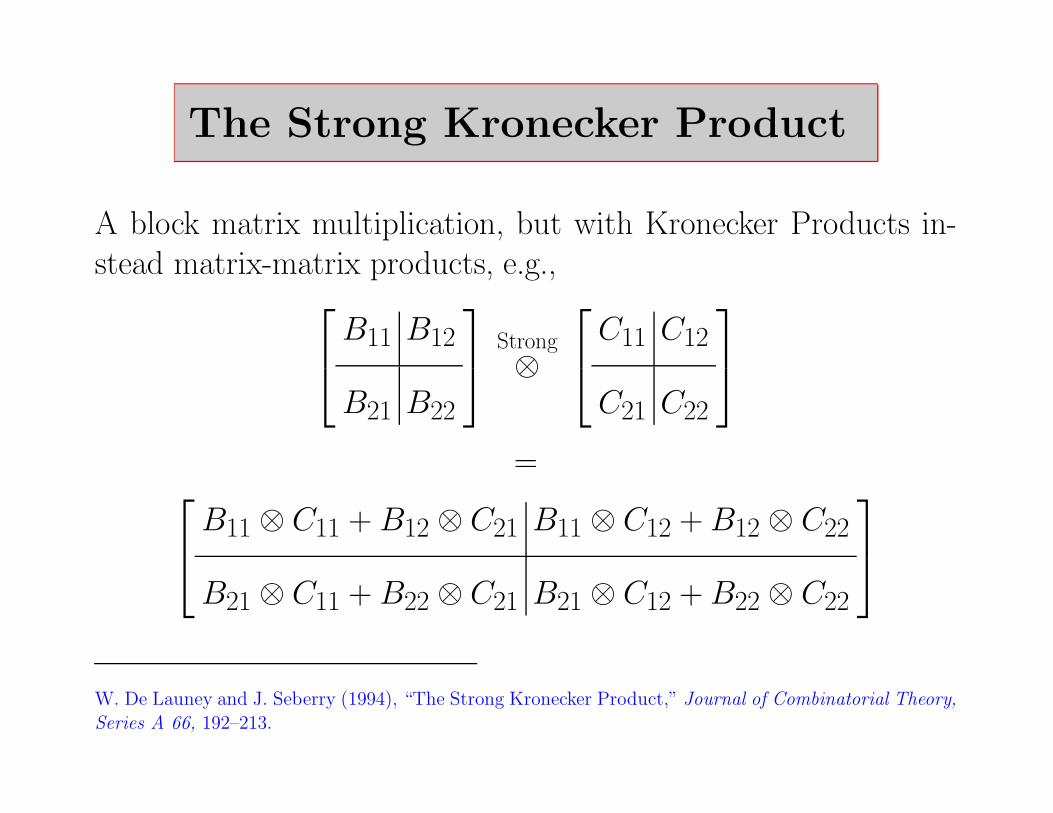
The Strong Kronecker Product
A block matrix multiplication, but with Kronecker Products in-stead matrix-matrix products, e.g.,
B11 B12
B21 B22
Strong⊗
C11 C12
C21 C22
=
B11 ⊗ C11 + B12 ⊗ C21 B11 ⊗ C12 + B12 ⊗ C22
B21 ⊗ C11 + B22 ⊗ C21 B21 ⊗ C12 + B22 ⊗ C22
W. De Launey and J. Seberry (1994), “The Strong Kronecker Product,” Journal of Combinatorial Theory,
Series A 66, 192–213.

The Symmetric Kronecker Product
The KP turns matrix equations into vector equations:
CXBT = G ⇔ (B ⊗ C) vec(X) = vec(G)
The symmetric Kronecker product does the same thing for matrixequations with symmetric solutions:
12
(
CXBT + BXCT)
= G (symmetric)
⇔
(Bsym⊗ C) svec(X) = svec(G)
where
svec
x11 x12 x13
x12 x22 x23
x13 x23 x33
=[
x11
√2x12 x22
√2x13
√2x23 x33
]T
F. Alizadeh, J-P.A. Haeberly, and M.L. Overton (1998). “Primal-Dual Interior Point Methods for Semidef-
inite Programming: Convergence Rates, Stability, and Numerical Results,” SIAM J. Optimization 8, 746–768.
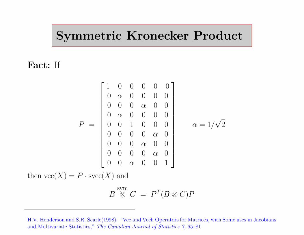
Symmetric Kronecker Product
Fact: If
P =
1 0 0 0 0 00 α 0 0 0 00 0 0 α 0 00 α 0 0 0 00 0 1 0 0 00 0 0 0 α 00 0 0 α 0 00 0 0 0 α 00 0 α 0 0 1
α = 1/√
2
then vec(X) = P · svec(X) and
Bsym⊗ C = P T (B ⊗ C)P
H.V. Henderson and S.R. Searle(1998). “Vec and Vech Operators for Matrices, with Some uses in Jacobians
and Multivariate Statistics,” The Canadian Journal of Statistics 7, 65–81.
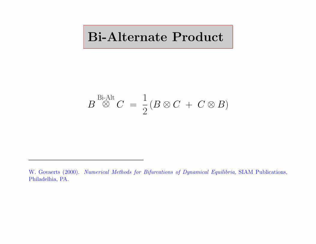
Bi-Alternate Product
BBi-Alt⊗ C =
1
2(B ⊗ C + C ⊗ B)
W. Govaerts (2000). Numerical Methods for Bifurcations of Dynamical Equilibria, SIAM Publications,Philadelhia, PA.

The 2000’sThree Predictions
©∞
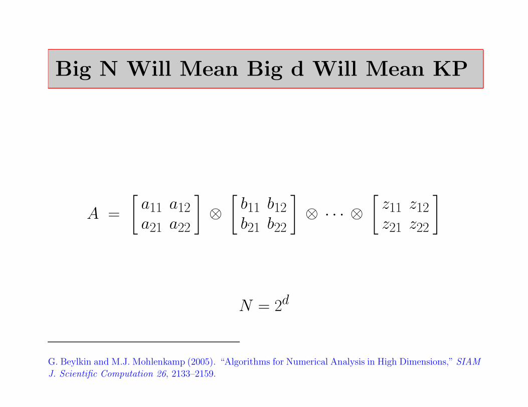
Big N Will Mean Big d Will Mean KP
A =
[
a11 a12a21 a22
]
⊗[
b11 b12b21 b22
]
⊗ · · · ⊗[
z11 z12z21 z22
]
N = 2d
G. Beylkin and M.J. Mohlenkamp (2005). “Algorithms for Numerical Analysis in High Dimensions,” SIAM
J. Scientific Computation 26, 2133–2159.
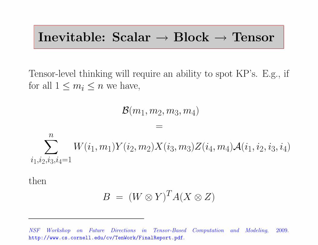
Inevitable: Scalar → Block → Tensor
Tensor-level thinking will require an ability to spot KP’s. E.g., iffor all 1 ≤ mi ≤ n we have,
B(m1,m2,m3,m4)
=n
∑
i1,i2,i3,i4=1
W (i1,m1)Y (i2,m2)X(i3,m3)Z(i4,m4)A(i1, i2, i3, i4)
then
B = (W ⊗ Y )TA(X ⊗ Z)
NSF Workshop on Future Directions in Tensor-Based Computation and Modeling, 2009.
http://www.cs.cornell.edu/cv/TenWork/FinalReport.pdf.

Data-Sparse Approximate Factorizations
New KP-based factorizations will widen the set of solvable hugeproblems.
Sample factorization...
A ≈ (B1 ⊗ C1)(B2 ⊗ C2)(B3 ⊗ C3) · · ·

Det(Log(A)) via Zehfuss
If
A ≈ (B ⊗ C)(D ⊗ E)(F ⊗ G) · · ·
then the big log det problem becomes a bunch of smaller ones...
log(det(A)) ≈nc log(det(B)) + nb log(det(C)) +
ne log(det(D)) + nd log(det(E)) +
ng log(det(F )) + nf log(det(G)) · · ·
R.P. Barry and R.K. Pace (1999). “Monte Carlo Estimates of the Log Determinant of Large Sparse
Matrices,” Linear Algebra and Its Applications 289, 41–54.


