Journal of Computations & Modelling, vol.5, no.3, 2015, 35-80
ISSN: 1792-7625 (print), 1792-8850 (online)
Scienpress Ltd, 2015
The Lindley Power Series Class of Distributions:
Model, Properties and Applications
Gayan Warahena-Liyanage1 and Mavis Pararai2
Abstract
The aim of this paper is to propose a new class of lifetime distributions
called the Lindley power series (LPS). The distribution properties including
survival function, hazard and reverse hazard functions, limiting behavior of
the pdf and hazard function, quantile function, moments, distribution of order
statistics, mean deviations, Lorenz and Bonferroni curves and Fisher informa-
tion are presented. The method of maximum likelihood estimation is used to
estimate the model parameters of this new class of distributions. The special
cases of the LPS distribution including Lindley binomial (LB), Lindley geo-
metric (LG), Lindley Poisson (LP) and Lindley logarithmic (LL) distributions
are presented. The Lindley logarithmic (LL) distribution is discussed in detail.
A Monte Carlo simulation study is presented to exhibit the performance and
accuracy of maximum likelihood estimates of the LL model parameters. Some
real data examples are discussed to illustrate the usefulness and applicability
of the LL distribution.
Mathematics Subject Classification:60E05; 62E99; 62P99
Keywords: Lindley power series distribution; Lindley logarithmic distribution;
Lindley distribution; Monte-Carlo simulation; Maximum likelihood estimation
1 Department of Mathematics, Indiana University of Pennsylvania, Indiana, PA, 15705, USA.E-mail: [email protected]
2 Department of Mathematics, Indiana University of Pennsylvania, Indiana, PA, 15705, USA.E-mail: [email protected]
Article Info: Received: April 12, 2015. Revised: May 15, 2015.Published online: June 10, 2015.
36 The Lindley Power Series Class of Distributions
1 Introduction
The modeling of lifetime data has become popular in the area of survival analy-
sis. In survival analysis, we study the lifetime of biological organisms or mechan-
ical systems. In recent years, many distributions have been introduced to model
these types of data. The basic concept behind introducing these distributions is that
the lifetime of a system withN number of components and a positive continuous
random variable,Xi, which denotes the lifetime of theith component, can be rep-
resented by a non-negative random variableZ=min(X1, X2, . . . , XN) if the com-
ponents are in a series orZ=max(X1, X2, . . . , XN) if the components are parallel.
Some of the well-known lifetime distributions include the exponential geometric
(EG) distribution by Adamidis and Loukas [1], exponential Poisson (EP) distribu-
tion by Kus [10], exponential logarithmic (EL) distribution by Tahmasbi and Rezaei
[22], Weibull geometric (WG) distribution by Barreto-Souza et al. [2] and Weibull
Poisson (WP) distribution by Lu and Shi [12].
Lindley [11] introduced a mixture of exponential and length-biased exponential
distributions to illustrate the difference between fiducial and posterior distributions.
This mixture is called the Lindley (L) distribution. Ghitany et al. [6] examined
and studied the properties and applications of the Lindley distribution in the context
of reliability analysis. The cumulative distribution function (cdf) of the Lindley
distribution is given by
GL(x; β) = 1−(
1 + β + βx
β + 1
)e−βx, x > 0, β > 0, (1)
and
gL(x; β) =β2
β + 1(1 + x)e−βx, x > 0, β > 0, (2)
respectively.
The survival function and hazard function of the Lindley distribution are given
by
SL(x; β) = GL(x; β) = 1−GL(x; β) =
(1 + β + βx
β + 1
)e−βx, (3)
and
hL(x; β) =gL(x; β)
GL(x; β)=
β2(1 + x)
(1 + β + βx), (4)

Gayan Warahena-Liyanage and Mavis Pararai 37
respectively, wherex > 0, α > 0, β > 0.
Using the transformationY = X1α , Ghitany et al. [5] derived the power Lindley
(PL) distribution and its properties.
Warahena-Liyanage and Pararai [23] studied the properties of the exponenti-
ated Power Lindley (EPL) distribution which modeled lifetime data better than the
Lindley and power Lindley distributions.
Another generalization of EPL distribution called the exponentiated power Lind-
ley Poisson (EPLP) distribution which is obtained by compounding the zero-inflated
Poisson distribution and the EPL distribution was derived and studied by Pararai et
al. [17].
Noack [16] proposed and studied the power series class of distributions. This
class of distributions includes binomial, geometric, logarithmic and Poisson distri-
butions as special cases. However, these distributions may not be useful when a
random variable takes the value of zero with high probability i.e. zero-inflated. In
such situations, it is more appropriate to consider the distribution which is truncated
at zero. More details on these distributions can be found in the context of univariate
discrete distributions by Johnson et al. [8].
In recent years, some authors have used the power series class of distributions to
develop new distributions. Many of these new distributions have been constructed
as a mixture of some well known distributions and the power series class of distri-
butions. Some of the power series distributions include the Weibull-power series
(WPS) distributions by Morais and Barreto-Souza [15], generalized exponential-
power series (GEPS) distributions by Mahmoudi and Jafari [13], Kumaraswamy-
power series (KPS) distributions by Bidram and Nekouhou [3], and Linear failure
rate-power series distributions by Mahamoudi and Jafari [14].
We provide three motivations for the new Lindley power series (LPS) class of
distributions, which can be applied in some interesting situations as follows:
(i) Due to the stochastic representationZ=min(X1, X2, . . . , XN) the LPS class
of distributions can arise in many industrial applications and biological or-
ganisms.
(ii) The LPS class of distributions can be used to model appropriately the time to
the first failure of a system of identical components that are in a series.
(iii) The LPS class of distributions exhibit some interesting behaviors with non-
monotonic failure rates such as bathtub, upside bathtub and increasing- decreasing-
38 The Lindley Power Series Class of Distributions
increasing failure rates which are more likely to be encountered in real life
situations.
The paper is organized as follows: In section 2, we present some basic informa-
tion on the Lindley distribution and the power series family of distributions. The
general model of the LPS class of distributions is defined and its properties includ-
ing hazard and reverse hazard functions, limiting behavior of the pdf and hazard
function, quantile function, moments, distribution of order statistics, mean devi-
ations, Lorenz and Bonferroni curves and Fisher information are presented. The
method of maximum likelihood estimation is used to estimate the model parame-
ters of this new class of distributions. In section 3, we introduce the special cases
of the LPS distribution including Lindley binomial (LB) distribution, Lindley geo-
metric (LG) distribution, Lindley Poisson (LP) distribution and Lindley logarithmic
(LL) distribution. The Lindley logarithmic (LL) distribution will be explored in
detail in section 4. The properties of the LL distribution such as survival func-
tion, hazard and reverse hazard functions, quantile function, moments, distribution
of order statistics, mean deviations, Lorenz and Bonferroni curves, reliability and
entropy measures are also presented. In section 5, we introduce some algorithms
for generating random data from LL distribution. A Monte Carlo simulation study
is also presented to exhibit the performance and accuracy of maximum likelihood
estimates of the LL model parameters. We present some real data examples in sec-
tion 6 to illustrate the usefulness and applicability of the LL distribution. Section 7
contains the conclusions and suggestions for further study.
2 The General Class and Properties
Let X1, X2, . . . , XN be independent and identically distributed (iid) random
variables from the Lindley (L) distribution whose cumulative distribution function
(cdf) and probability density function (pdf) are given by equations (1) and (2), re-
spectively.
ConsiderN to be a discrete random variable from a power series distribution
(truncated at zero) and whose pdf is given by
P (N = n) =anλ
n
C(λ), n = 1, 2, 3, . . . , (5)

Gayan Warahena-Liyanage and Mavis Pararai 39
whereC(λ) =∞∑
n=1
anλn andan depends onn andλ > 0. C(λ) is finite and its first,
second and third derivatives with respect toλ are defined and given byC ′(.), C ′′(.)
andC ′′′(.), respectively. The power series family of distributions includes bino-
mial, Poisson, geometric and logarithmic distributions as defined in Johnson et al.
[8]. Table 1 represents some useful quantities includingan, C(λ), C(λ)−1, C ′(λ),
C ′′(λ), andC ′′′(λ) for the Poisson, geometric, logarithmic and binomial (withm
being the number of replicas) distributions.
Table 1: Useful quantities for some power series distributions
Distribution C(λ) C ′(λ) C ′′(λ) C ′′′(λ) C−1(λ) an Parameter Space
Poisson eλ − 1 eλ eλ eλ log(1 + λ) (n!)−1 (0,∞)
Geometric λ(1− λ)−1 (1− λ)−2 2(1− λ)−3 6(1− λ)−4 λ(1 + λ)−1 1 (0, 1)
Logarithmic − log(1− λ) (1− λ)−1 (1− λ)−2 2(1− λ)−3 1− e−λ n−1 (0, 1)
Binomial (1 + λ)m − 1m
(1 + λ)1−m
m(m− 1)
(1 + λ)2−m
m(m− 1)(m− 2)
(1 + λ)3−m(λ + 1)1/m − 1
(mn
)(0,∞)
Let X(1) = min(X1, X2, . . . , XN). The conditional cdf ofX(1) | N = n is given
by
GX(1)|N=n(x) = 1− [G(x)]n = 1−(
1 + β + βx
β + 1
)n
e−βnx, x > 0, (6)
whereG(.) is the survival function in Equation (3). The cdf of the new LPS class
of distributions is the marginal cdf ofX(1) which is given by
FLPS(x; β, λ) = 1−C[λ(
1+β+βxβ+1
)e−βx
]C(λ)
, (7)
wherex > 0, β > 0 andλ > 0.
2.1 Density function
The pdf of a random variableX from a LPS class of distributions whose cdf is
in (7) is given by
40 The Lindley Power Series Class of Distributions
fLPS(x; β, λ) = λβ2(β + 1)−1(1 + x)e−βxC ′[λ(
1+β+βxβ+1
)e−βx
]C(λ)
, (8)
wherex > 0, β > 0, andλ > 0.
The following propositions discuss the limiting behavior and some other char-
acteristics of the LPS distribution.
Proposition 2.1. The Lindley distribution is a limiting distribution of the LPS
distribution whenλ → 0+.
Proof. Applying C(λ) =∞∑
n=1
anλn in (7), we obtain
limλ→0+
FLPS(x) = 1− limλ→0+
∞∑n=1
an
[λ(
1+β+βxβ+1
)e−βx
]n∑∞
n=1 anλn.
By using L’Hopital’s rule, we obtain
limλ→0+
FLPS(x) = 1− limλ→0+
a1
(1+β+βx
β+1
)e−βx +
∞∑n=2
nanλn−1(
1+β+βxβ+1
)n
e−nβx
a1 +∑∞
n=2 nanλn−1
= 1−(
1 + β + βx
β + 1
)e−βx.
Proposition 2.2. The density function of LPS class can be expressed as a linear
combination of the density ofX(1) =min(X1, X2, . . . , Xn).
Proof. SinceC ′(λ) =∞∑
n=1
nanλn−1, we have
fLPS(x) =∞∑
n=1
P (N = n)gX(1)(x; n),
wheregX(1)(x; n) is the probability pdf ofX(1) =min(X1, X2, . . . , Xn) given by
gX(1)(x; n) =
nβ2
(β + 1)n(1 + β + βx)n−1(1 + x)e−nβx. (9)
Gayan Warahena-Liyanage and Mavis Pararai 41
Proposition 2.3. For the pdf of the LPS distribution, we have
limx→0+
fLPS(x) =λβ2C ′(λ)
(β + 1)C(λ),
and
limx→∞
fLPS(x) = 0.
2.2 Reverse hazard and hazard functions
The reverse hazard function and the hazard function of the LPS distribution,
respectively, are given by
τLPS(x; β, λ) = λβ2(β + 1)−1(1 + x)e−βxC ′[λ(
1+β+βxβ+1
)e−βx
]C(λ)− C
[λ(
1+β+βxβ+1
)e−βx
] ,(10)
and
hLPS(x; β, λ) = λβ2(β + 1)−1(1 + x)e−βxC ′[λ(
1+β+βxβ+1
)e−βx
]C[λ(
1+β+βxβ+1
)e−βx
] ,
(11)
wherex > 0, β > 0 andλ > 0.
The following Proposition gives the limiting behavior of the hazard function of
the LPS distribution in (11).
Proposition 2.4. For the hazard function of the LPS distribution, we have
limx→0+
hLPS(x) =λβ2C ′(λ)
(β + 1)C(λ),
and
limx→∞
hLPS(x) = ∞.

42 The Lindley Power Series Class of Distributions
2.3 Quantile function
In this section, the quantile function of the LPS distribution will be derived. The
quantile function,Q(p), defined byFLPS(Q(p)) = p is the root of the equation,
1−C[λ(
1+β+βQ(p)β+1
)e−βQ(p)
]C(λ)
= p, where0 < p < 1.
Let Z(p) = −1− β − βQ(p), then we have
1−C[λ(
Z(p)β+1
)eZ(p)+β+1)
]C(λ)
= p.
That is,
Z(p)eZ(p) = −(β + 1)C−1((1− p)C(λ))
λeβ+1
whereC−1(.) is the inverse function ofC(.) Then solution forZ(p) is
Z(p) = W
[−(β + 1)C−1((1− p)C(λ))
λeβ+1
],
for 0 < p < 1, whereW (.) is the negative branch of the LambertW function. See
Corless et.al [4] for history, theory and applications of the LambertW function.
Consequently, the quantile function of the LPS distribution is given by
Q(p) = −1− 1
β− 1
βW
[−(β + 1)C−1((1− p)C(λ))
λeβ+1
], where0 < p < 1.
(12)
2.4 Moments and related measures
In this section, moments and related measures such as coefficient of variation,
skewness and kurtosis of the LPS distribution are presented. In order to find the
moments, the following Lemma is proved.

Gayan Warahena-Liyanage and Mavis Pararai 43
Lemma 2.5. Let
L1(β, n, p) =
∞∫0
xp(1 + x)(1 + β + βx)n−1e−nβxdx,
then
L1(β, n, p) =n−1∑i=0
i+1∑j=0
(n− 1
i
)(i + 1
j
)Γ(j + p + 1)
nj+p+1βp+j−i+1.
Proof. Using the series expansion for|z| < 1 anda > 0,
(1− z)a−1 =∞∑i=0
(a− 1
i
)(−1)izi. (13)
Usingz = β(1 + x), we have,
L1(β, n, p) =
∞∫0
xp(1 + x)(1 + β(1 + x))n−1e−nβxdx
=n−1∑i=0
i+1∑j=0
(n− 1
i
)(i + 1
j
)βi
∞∫0
xj+pe−nβxdx.
Consequently,
L1(β, n, p) =n−1∑i=0
i+1∑j=0
(n− 1
i
)(i + 1
j
)Γ(j + p + 1)
nj+p+1βp+j−i+1. (14)
The rth moment of a random variableX from the LPS distribution, sayµ′r, is
given by
µ′r = E(Xr) =
∞∫0
xrfLPS(x)dx.
44 The Lindley Power Series Class of Distributions
Using the fact in Proposition (2.2), we have
E(Xr) =∞∑
n=1
P (N = n)E(Xr(1)) =
∞∑n=1
P (N = n)
∞∫0
xrgX(1)(x; n)dx
=∞∑
n=1
P (N = n)nβ2
(β + 1)n
∞∫0
xr(1 + x)(1 + β + βx)n−1e−nβxdx.
Using Lemma (2.5), it follows that
E(Xr) =∞∑
n=1
P (N = n)nβ2L1(β, n, r)
(β + 1)n.
Consequently, therth moment of the LPS distribution is given by
µ′r = E(Xr) =∞∑
n=1
anλn
C(λ)
nβ2L1(β, n, r)
(β + 1)n. (15)
The mean (µ), variance(σ2), coefficient of variation (CV), coefficient of skew-
ness (CS), and coefficient of kurtosis (CK) are given by
µ = E(X) =∞∑
n=1
anλn
C(λ)
nβ2L1(β, n, 1)
(β + 1)n, (16)
σ2 = µ′2 − µ2, (17)
CV =σ
µ=
√µ′2 − µ2
µ=
√µ′2µ2− 1, (18)
CS =E [(X − µ)3]
[E(X − µ)2]3/2=
µ′3 − 3µµ′2 + 2µ3
(µ′2 − µ2)3/2, (19)
and
CK =E [(X − µ)4]
[E(X − µ)2]2=
µ′4 − 4µµ′3 + 6µ2µ′2 − 3µ4
(µ′2 − µ2)2. (20)
Gayan Warahena-Liyanage and Mavis Pararai 45
2.5 Conditional moments
For lifetime models, it is useful to study the conditional moments which are
defined asE(Xr | X > x). The following Lemma is introduced to evaluate condi-
tional moments.
Lemma 2.6. Let
L2(β, n, p, t) =
∞∫t
xp(1 + x)(1 + β + βx)n−1e−nβxdx,
then
L2(β, n, p, t) =n−1∑i=0
i+1∑j=0
(n− 1
i
)(i + 1
j
)Γ(j + p + 1, nβt)
nj+p+1βp+j−i+1.
Proof. Applying the series expansion in Equation (13) withz = β(1+x) we obtain,
L2(β, n, p, t) =
∞∫0
xp(1 + x)(1 + β(1 + x))n−1e−nβxdx
=n−1∑i=0
i+1∑j=0
(n− 1
i
)(i + 1
j
)βi
∞∫t
xj+pe−nβxdx.
Consequently,
L2(β, n, p, t) =n−1∑i=0
i+1∑j=0
(n− 1
i
)(i + 1
j
)Γ(j + p + 1, nβt)
nj+p+1βp+j−i+1. (21)
Using Proposition (2.2) and Lemma (2.6), the rth conditional moment of the
LPS distribution is given by
E(Xr | X > x) =∞∑
n=1
P (N = n)nβ2
(β + 1)n
L2(β, n, r, x)
1− FLPS(x)
=∞∑
n=1
anλn
C(λ(
1+β+βxβ+1
)e−βx
) nβ2L2(β, n, r, x)
(β + 1)n. (22)
46 The Lindley Power Series Class of Distributions
2.6 Moment generating function
The moment generating function (MGF) of the LPS distribution is defined by
MX(t) = E(etX).
By considering the fact in Proposition (2.2), we obtain
MX(t) =∞∑
n=1
P (N = n)MX(1)(t) =
∞∑n=1
P (N = n)
∞∫0
etxgX1(x; n)dx. (23)
Using the series expansionetx =∞∑
k=0
tkxk
k!and Lemma (2.5) in Equation (23), the
moment generating function (MGF) of the LPS distribution is given by
MX(t) =∞∑
n=1
∞∑k=0
anλn
C(λ)
nβ2tkL1(β, n, k)
(β + 1)nk!. (24)
2.7 Distribution of order statistics
Let X1, X2, . . . , Xn be a random sample from the LPS distribution and suppose
X1:n < X2:n < . . . < Xn:n denote the corresponding order statistics. The pdf of the
kth order statistic is given by
fk:n(x)n!
(k − 1)!(n− k)!f(x)[F (x)]k−1[1− F (x)]n−k, (25)
whereF (.) andf(.) are the cdf and pdf of LPS distributions given in equations (7)
and (8), respectively. Using the series expansion in Equation (13), we can re-write
Equation (25) as follows:
fk:n(x) =n!
(k − 1)!(n− k)!
n−k∑l=0
(n− k
l
)(−1)lf(x)[F (x)]k+l−1. (26)
Note that,
f(x)[F (x)]k+l−1 =1
k + l
d
dx[F (x)]k+l.

Gayan Warahena-Liyanage and Mavis Pararai 47
The corresponding cdf offk:n(x), denoted byFk:n(x) can be obtained as
Fk:n(x) =n!
(k − 1)!(n− k)!
n−k∑l=0
(n−k
l
)(−1)l
k + l[F (x)]k+l
=n!
(k − 1)!(n− k)!
n−k∑l=0
(n−k
l
)(−1)l
k + l
1−C(λ(
1+β+βxβ+1
)e−βx
)C(λ)
k+l
=n!
(k − 1)!(n− k)!
n−k∑l=0
(n−k
l
)(−1)l
k + lFG(x; β, λ, k + l),
whereG follows an exponentiated LPS (ELPS) distribution with parametersβ, λ
and k + l. Thus, the cdf of thekth order statistic can be expressed as a linear
combination of the cdf of the ELPS distribution with parametersβ, λ andk + l.
2.8 Mean deviations
In this section, the mean deviation about the mean and the mean deviation about
the median of the LPS distribution are presented. The amount of scatter in a pop-
ulation can be measured by the totality of deviations from the mean and median.
The mean deviation about the mean, sayD(µ), and the mean deviation about the
median, sayD(M), are defined as
D(µ) =
∞∫0
| x− µ | fLPS(x)dx, D(M) =
∞∫0
| x−M | fLPS(x)dx,
respectively, whereµ = E(X) andM = Median(X) = F−1(1/2) is the median
of FLPS. The measuresD(µ) and D(M) can be evaluated using the following
relationships:
D(µ) = 2µFLPS(µ)− 2µ + 2
∞∫µ
xfLPS(x), (27)
and
D(M) = −µ + 2
∞∫M
xfLPS(x). (28)
48 The Lindley Power Series Class of Distributions
Using Lemma (2.6), we obtain
D(µ) = 2µFLPS(µ)− 2µ + 2∞∑
n=1
anλn
C(λ)
nβ2L2(β, n, 1, µ)
(β + 1)n,
and
D(M) = −µ + 2∞∑
n=1
anλn
C(λ)
nβ2L2(β, n, 1, M)
(β + 1)n.
2.9 Lorenz and Bonferroni curves
In this section, the Lorenz and Bonferroni curves for the LPS distribution are
presented. The Lorenz and Bonferroni curves have a number of applications in
different fields such as medicine, income and poverty, reliability and insurance.
The Lorenz and Bonferroni curves are given by
L(FLPS(x)) =
x∫0
tfLPS(t)dt
E(X), and B(FLPS(x)) =
L(FLPS(x))
FLPS(X),
or
L(p) =1
µ
q∫0
xfLPS(x)dx, and B(p) =1
pµ
q∫0
xfLPS(x)dx, (29)
respectively, whereq = F−1LPS(p). Applying Lemma (2.6) in (29), we obtain
L(p) =1
µ
(µ−
∞∑n=1
anλn
C(λ)
nβ2L2(β, n, 1, q)
(β + 1)n
), (30)
and
B(p) =1
pµ
[µ−
∞∑n=1
anλn
C(λ)
nβ2L2(β, n, 1, q)
(β + 1)n
]. (31)
Gayan Warahena-Liyanage and Mavis Pararai 49
2.10 Maximum likelihood estimation
In this section, the maximum likelihood method used in estimating the parame-
tersβ andλ is presented. Letx1, x2, . . . , xn ben observations of a random sample
from LPS distribution andΘ = (β, λ)T be the unknown parameter vector. From
Equation (8), the log-likelihood function of LPS distribution is given by
ln(β, λ) = n log(λ) + 2n log(β)− n log(β + 1)− n log(C(λ)) +n∑
i=1
log(1 + xi)
−β
n∑i=1
xi +n∑
i=1
log
{C ′[λ
(1 + β + βxi
β + 1
)e−βxi
]}. (32)
The associated score function isUn(Θ) =(
∂ln∂β
, ∂ln∂λ
)T
, where∂ln∂β
and ∂ln∂λ
are the
partial derivatives of the log-likelihood function given by
∂ln∂β
=2n
β− n
β + 1−
n∑i=1
xi −n∑
i=1
λxie−βxi [(1 + β + βxi)(β + 1)− 1]
(β + 1)2
×C ′′[λ(
1+β+βxi
β+1
)e−βxi
]C ′[λ(
1+β+βxi
β+1
)e−βxi
] , (33)
and
∂ln∂λ
=n
λ− nC ′(λ)
C(λ)+
n∑i=1
(1 + β + βxi)e−βxi
β + 1
C ′′[λ(
1+β+βxi
β+1
)e−βxi
]C ′[λ(
1+β+βxi
β+1
)e−βxi
] , (34)
respectively. The maximum likelihood estimates ofΘ can be obtained by solving
the non-linear systemUn(Θ) = 0. Since the equations (33) and (34) are not in
closed form, the solutions can be found by using a numerical method such as the
Newton-Raphson procedure.
2.11 Fisher information matrix and asymptotic confidence in-
tervals
In this section, we present a measure for the amount of information. This in-
formation can be used for interval estimation and hypothesis testing for the model
50 The Lindley Power Series Class of Distributions
parametersβ andλ.
LetX be a random variable with the LPS pdffLPS(·; Θ), whereΘ = (θ1, θ2)T =
(β, λ)T . The Fisher information matrix (FIM) is the2 × 2 symmetric matrix given
by
I(Θ) =
[Iββ Iβλ
Iλβ Iλλ
],
where elementsIij(Θ) = −EΘ
[∂2 log(fLPS(X;Θ))
∂θi∂θj
]. The elements of the FIM can be
obtained by considering the second order partial derivatives of (32). These elements
can be numerically obtained by MATLAB or MAPLE software. The total FIM
In(Θ) can be approximated by
Jn(Θ) ≈[− ∂2 log L
∂θi∂θj
∣∣∣∣Θ=Θ
]2×2
(35)
For real data, the matrix given in Equation (35) is obtained after the convergence
of the Newton-Raphson procedure in MATLAB or R software. LetΘ = (β, λ)
be the maximum likelihood estimate ofΘ = (β, λ). Under the usual regularity
conditions and that the parameters are in the interior of the parameter space, but not
on the boundary, we have:√
n(Θ−Θ)d−→ N2(0, I
−1(Θ)), whereI(Θ)
is the expected Fisher information matrix. The asymptotic behavior is still valid
if I(Θ) is replaced by the observed information matrix evaluated atΘ, that isJ(Θ).
The multivariate normal distribution with mean vector0 = (0, 0)T and covariance
matrix I−1(Θ) can be used to construct confidence intervals for the model parame-
ters. The approximate100(1− η)% two-sided confidence intervals forβ andλ are
given by
β ± Zη/2
√I−1ββ (Θ), and λ± Zη/2
√I−1λλ (Θ),
respectively, whereI−1ββ (Θ), andI−1
λλ (Θ) are diagonal elements ofI−1n (Θ) = (nIΘ))−1
andZη/2 is the upper(η/2)th percentile of a standard normal distribution.
3 Special Cases of LPS Class of Distributions
In this section, we study some special cases of the LPS class of distributions

Gayan Warahena-Liyanage and Mavis Pararai 51
including Lindley binomial (LB) distribution, Lindley geometric (LG) distribution,
Lindley Poisson (LP) distribution, and Lindley logarithmic (LL) distribution. The
LG and LP distributions were introduced and studied as two separate studies by
Zakerzadeh and Mahmoudi [24], and Gui et al. [7], respectively. We present an
overview of the LB, LG and LP distributions as special cases of the LPS class and
discuss the LL distribution in detail in the following sections.
3.1 Lindley binomial distribution
The binomial distribution (truncated at zero) is a special case of the class of
power series distributions withan =(
mn
)andC(λ) = (1 + λ)m − 1, wherem(n 6
m) is the number of replicas. From Equation (7), the cdf of the Lindley binomial
(LB) distribution is given by
FLB(x; β, λ, m) = 1−
[1 + λ
(1+β+βx
β+1
)e−βx
]m− 1
(1 + λ)m − 1, x > 0, β > 0, λ > 0,
(36)
wherem is a positive integer.
The associated pdf is given by
fLB(x; β, λ, m) =mλβ2(1 + x)e−βx
[1 + λ
(1+β+βx
β+1
)e−βx
]m−1
(β + 1)[(1 + λ)m − 1], (37)
wherex > 0, β > 0, λ > 0, andm is a positive integer.
3.2 Lindley geometric distribution
The Lindley geometric (LG) distribution was introduced and studied by Zak-
erzadeh and Mahmoudi [24]. The cdf and pdf of the LG distribution are presented
to show that it is a special case of LPS class. Using Equation (7) withan = 1 and
C(λ) = λ(1− λ)−1, the cdf of the LG distribution is given by
FLG(x; β, λ) =1−
(1+β+βx
β+1
)e−βx
1− λ(
1+β+βxβ+1
)e−βx
, x > 0, β > 0, 0 < λ < 1. (38)
52 The Lindley Power Series Class of Distributions
The pdf of the LG distribution is given by
fLG(x; β, λ) =β2(1− λ)(1 + x)e−βx
(β + 1)[1− λ
(1+β+βx
β+1
)e−βx
]2 , x > 0, β > 0, 0 < λ < 1.
(39)
The LG distribution was fitted to two real data sets. The first data set consists
of waiting times (in minutes) before service of 100 bank customers. The second
data set consisted of vinyl chloride data obtained from clean upgradient monitoring
wells in mg/L. For each data set the LG distribution proved to be superior to all the
other models it was compared to.
3.3 Lindley Poisson distribution
The Lindley Poisson (LP) distribution was introduced and studied by Gui et al.
[7]. Using the stochastic representationX(n) = max(X1, X2, . . . , XN), Pararai et
al. [17] introduced the exponentiated power Lindley Poisson (EPLP) distribution
for which the LP distribution is a submodel. The cdf and pdf of the LP distribution
are presented to show that it is a special case of LPS class. Using Equation (7) with
an = 1/n! andC(λ) = eλ − 1, whereλ > 0, the cdf of the LP distribution is given
by
FLP (x; β, λ) =eλ − eλ( 1+β+βx
β+1 )e−βx
eλ − 1, x > 0, β > 0, λ > 0. (40)
The LP distribution was fitted to two real data sets. The first data set consisted
of time intervals of the successive earthquakes taken from University of Bosphoros,
Kandilli Observatory and Earthquake Research Institute-National Earthquake Mon-
itoring Center. The second data set consists of survival times of guinea pigs injected
with different doses of tubercle bacilli. For each data set the LP distribution proved
to be superior to all the other models it was compared to.
The corresponding pdf is given by
fLP (x; β, λ) =λβ2(1 + x)eλ( 1+β+βx
β+1 )e−βx−βx
(β + 1)(eλ − 1), x > 0, β > 0, λ > 0. (41)
Gayan Warahena-Liyanage and Mavis Pararai 53
4 Lindley Logarithmic Distribution
In this section, the Lindley logarithmic (LL) distribution is introduced as a spe-
cial case of LPS class of distributions and will be studied in detail. The properties of
the LL distribution are derived from the properties of the general class. The entropy
measures and the reliability of the LL distribution are also presented.
4.1 The model
The LL distribution is defined by using the cdf of LPS distribution given in
Equation (7) withan = 1/n, andC(λ) = − log(1− λ), where0 < λ < 1. The cdf
and pdf of LL distribution are given by
FLL(x; β, λ) = 1−log(1− λ
(1+β+βx
β+1
)e−βx
)log(1− λ)
, (42)
and
fLL(x; β, λ) =λβ2(1 + x)e−βx
(β + 1) log(1− λ)[λ(
1+β+βxβ+1
)e−βx − 1
] , (43)
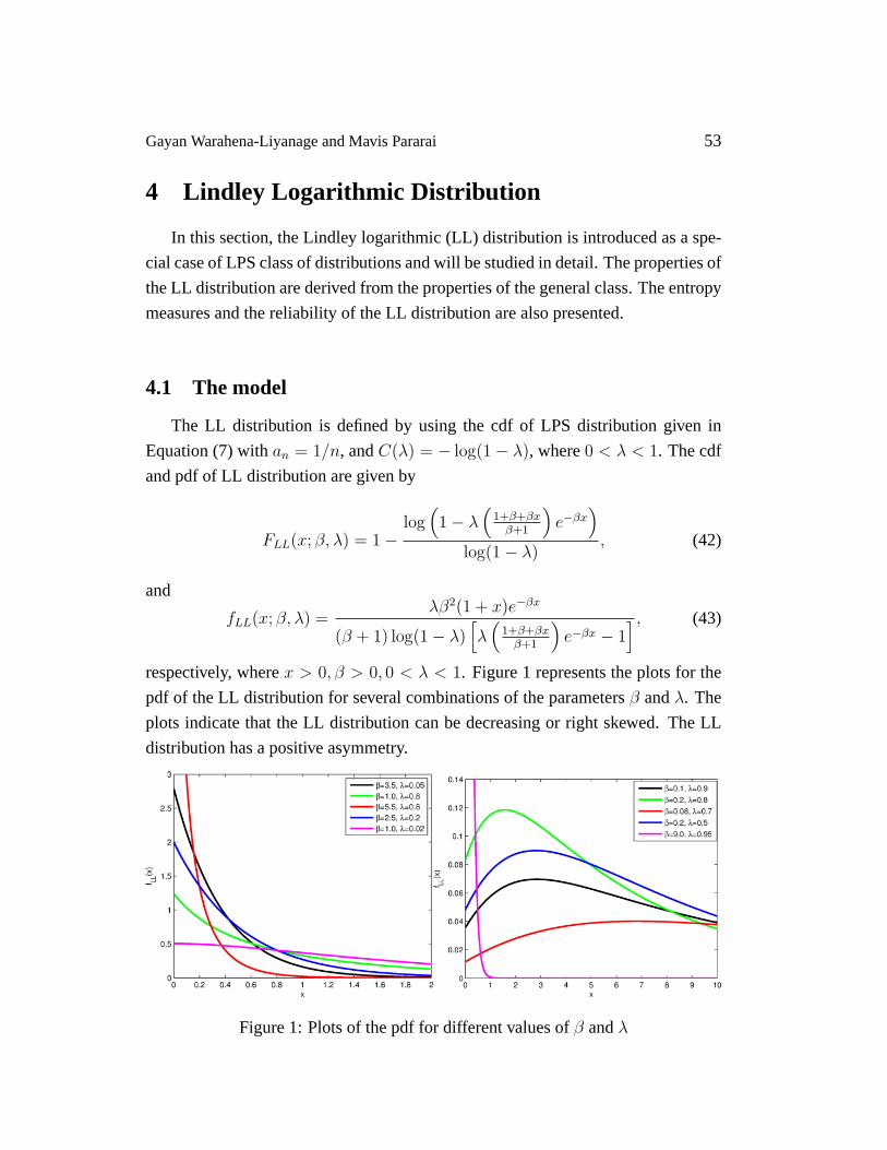
respectively, wherex > 0, β > 0, 0 < λ < 1. Figure 1 represents the plots for the
pdf of the LL distribution for several combinations of the parametersβ andλ. The
plots indicate that the LL distribution can be decreasing or right skewed. The LL
distribution has a positive asymmetry.
Figure 1: Plots of the pdf for different values ofβ andλ

54 The Lindley Power Series Class of Distributions
4.2 Quantile function
By substitutingC−1(λ) = 1 − e−λ in Equation (12), the quantile function for
the LL distribution is given as
Xq = −1− 1
β− 1
βW
(−(β + 1)(1− e(1−p) log(1−λ))
λeβ+1
), 0 < p < 1, (44)
whereW (.) is the negative branch of the LambertW function.
4.3 Reverse hazard and hazard functions
The reverse hazard function and hazard function of the LL distribution are re-
spectively given as follows:
from Equation (10)
τLL(x; β, λ) = λβ2(β +1)−1(1+x)e−βx
[1− λ
(1+β+βx
β+1
)e−βx
]−1
log[1− λ
(1+β+βx
β+1
)e−βx
]− log(1− λ)
,
(45)
and from Equation (11)
hLL(x; β, λ) = λβ2(β + 1)−1(1 + x)e−βx
[λ(
1+β+βxβ+1
)e−βx − 1
]−1
log(1− λ
(1+β+βx
β+1
)e−βx
) , (46)
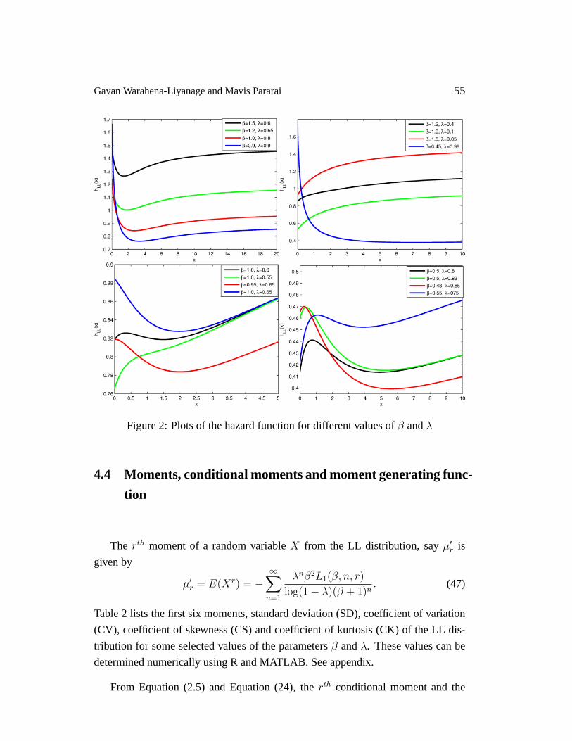
wherex > 0, β > 0 and0 < λ < 1. Plots of the hazard function of the LL dis-
tribution for several combinations of the parametersβ andλ are given in Figure
2. The plots for the hazard function of LL distribution exhibit different shapes in-
cluding monotonically increasing, monotonically decreasing, bathtub, upside down
bathtub and increasing-decreasing-increasing shapes. These interesting shapes of
the hazard function imply that LL distribution is suitable for monotonic and non-
monotonic hazard behaviors which are more likely to be encountered in real life
situations.
Gayan Warahena-Liyanage and Mavis Pararai 55
Figure 2: Plots of the hazard function for different values ofβ andλ
4.4 Moments, conditional moments and moment generating func-
tion
The rth moment of a random variableX from the LL distribution, sayµ′r is
given by
µ′r = E(Xr) = −∞∑
n=1
λnβ2L1(β, n, r)
log(1− λ)(β + 1)n. (47)
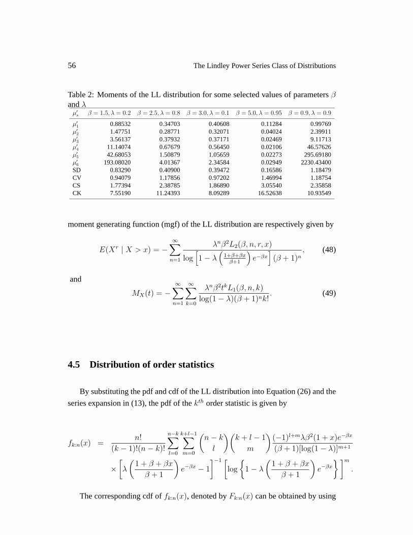
Table 2 lists the first six moments, standard deviation (SD), coefficient of variation
(CV), coefficient of skewness (CS) and coefficient of kurtosis (CK) of the LL dis-
tribution for some selected values of the parametersβ andλ. These values can be
determined numerically using R and MATLAB. See appendix.
From Equation (2.5) and Equation (24), therth conditional moment and the
56 The Lindley Power Series Class of Distributions
Table 2: Moments of the LL distribution for some selected values of parametersβandλ
µ′s β = 1.5, λ = 0.2 β = 2.5, λ = 0.8 β = 3.0, λ = 0.1 β = 5.0, λ = 0.95 β = 0.9, λ = 0.9
µ′1 0.88532 0.34703 0.40608 0.11284 0.99769µ′2 1.47751 0.28771 0.32071 0.04024 2.39911µ′3 3.56137 0.37932 0.37171 0.02469 9.11713µ′4 11.14074 0.67679 0.56450 0.02106 46.57626µ′5 42.68053 1.50879 1.05659 0.02273 295.69180µ′6 193.08020 4.01367 2.34584 0.02949 2230.43400SD 0.83290 0.40900 0.39472 0.16586 1.18479CV 0.94079 1.17856 0.97202 1.46994 1.18754CS 1.77394 2.38785 1.86890 3.05540 2.35858CK 7.55190 11.24393 8.09289 16.52638 10.93549
moment generating function (mgf) of the LL distribution are respectively given by
E(Xr | X > x) = −∞∑
n=1
λnβ2L2(β, n, r, x)
log[1− λ
(1+β+βx
β+1
)e−βx
](β + 1)n
, (48)
and
MX(t) = −∞∑
n=1
∞∑k=0
λnβ2tkL1(β, n, k)
log(1− λ)(β + 1)nk!. (49)
4.5 Distribution of order statistics
By substituting the pdf and cdf of the LL distribution into Equation (26) and the
series expansion in (13), the pdf of thekth order statistic is given by
fk:n(x) =n!
(k − 1)!(n− k)!
n−k∑l=0
k+l−1∑m=0
(n− k
l
)(k + l − 1
m
)(−1)l+mλβ2(1 + x)e−βx
(β + 1)[log(1− λ)]m+1
×[λ
(1 + β + βx
β + 1
)e−βx − 1
]−1 [log
{1− λ
(1 + β + βx
β + 1
)e−βx
}]m
.
The corresponding cdf offk:n(x), denoted byFk:n(x) can be obtained by using

Gayan Warahena-Liyanage and Mavis Pararai 57
Equation (27) and it is given by
Fk:n(x) =n!
(k − 1)!(n− k)!
n−k∑l=0
(n−k
l
)(−1)l
k + l
1−log{
1− λ(
1+β+βxβ+1
)e−βx
}log(1− λ)
k+l
=n!
(k − 1)!(n− k)!
n−k∑l=0
(n−k
l
)(−1)l
k + lFG(x; β, λ, k + l),
whereG follows an exponentiated Lindley logarithmic (ELL) distribution with pa-
rametersβ, λ andk + l. Thus, the cdf of thekth order statistic can be expressed
as a linear combination of the cdf of the ELL distribution with parametersβ, λ and
k + l.
4.6 Measures of uncertainty
In this section, the measures of uncertainty including Shannon [20],[21] entropy
and Renyi [19] entropy of the LL distribution are presented. The concept of entropy
plays an important role in information theory. The entropy of a random variable is
defined using its probability distribution and can be considered as a good measure
of randomness or uncertainty.
4.6.1 Shannon entropy
The Shannon entropy of the LL distribution is defined byH[fLL] =
E[− log(fLL(X; β, λ))]. Thus, we have
H[fLL] = E
[− log
{−λβ2(1 + X)e−βX
(β + 1) log(1− λ)
(1− λ
(1 + β + βX
β + 1
)e−βX
)−1}]
= − log
(−λβ2
(β + 1) log(1− λ)
)− E[log(1 + X)] + βE[X]
+E
[log
{1− λ
(1 + β + βX
β + 1
)e−βX
}]. (50)
We evaluateE[log(1 + X)], E[X], andE[log(1− λ
(1+β+βX
β+1
)e−βX
)]sepa-
58 The Lindley Power Series Class of Distributions
rately . Consider the series expansion
log(1 + z) =∞∑
q=1
(−1)q+1zq
qfor | z |< 1. (51)
Using the series expansion in Equation (51) withz = X and Equation (47), we have
E[log(1 + X)] =∞∑
q=1
(−1)q+1
qE[Xq] =
∞∑q=1
∞∑n=1
(−1)q+1λnβ2L1(β, n, q)
q log(1− λ)(β + 1)n. (52)
From Equation (47), we have
E[X] =∞∑
n=1
λnβ2L1(β, n, 1)
log(1− λ)(β + 1)n. (53)
ConsiderE[log(1− λ
(1+β+βX
β+1
)e−βX
)]and letV =
[1− λ
(1+β+βX
β+1
)e−βX
].
Note thatlog(V ) = log[1 + (V − 1)]. Using Equation (51) withz = (V − 1), we
obtain
log(V ) =∞∑
p=1
(−1)p+1(V − 1)p
p= −
∞∑p=1
(1− V )p
p.
Using the series expansion in Equation (13), we have
E[log(V )] =∞∑
p=1
p∑r=0
(p
r
)(−1)r+1E[V r]
p
=∞∑
p=1
p∑r=0
(p
r
)(−1)r+1
pE
[(1− λ
(1 + β + βX
β + 1
)e−βX
)r]
=∞∑
p=1
p∑r=0
r∑s=0
s∑t=0
t∑u=0
(p
r
)(r
s
)(s
t
)(t
u
)(−1)r+s+1λsβt
p(β + 1)sE[Xue−βsX
].
(55)
Note thatE[Xue−βsX
]=
∞∑v=0
(−1)vβvsvE[Xv+u]v!
. Thus, we have
E[log(V )] =∞∑
p=1
p∑r=0
r∑s=0
s∑t=0
t∑u=0
∞∑v=0
(p
r
)(r
s
)(s
t
)(t
u
)(−1)r+s+v+1λssvβt+v
pv!(β + 1)sE[Xu+v].

Gayan Warahena-Liyanage and Mavis Pararai 59
Using Equation (47), we obtain
E[log(V )] =∞∑
p=1
p∑r=0
r∑s=0
s∑t=0
t∑u=0
∞∑v=0
∞∑n=1
(p
r
)(r
s
)(s
t
)(t
u
)×(−1)r+s+v+1λs+nsvβt+v+2L1(β, n, u + v)
pv! log(1− λ)(β + 1)s+n. (56)
Substituting equations (52), (53), and (56) in Equation (50), we have
H[fLL] = − log
(−λβ2
(β + 1) log(1− λ)
)−
∞∑q=1
∞∑n=1
(−1)q+1λnβ2L1(β, n, q)
q log(1− λ)(β + 1)n
+∞∑
n=1
λnβ3L1(β, n, 1)
log(1− λ)(β + 1)n+
∞∑p=1
p∑r=0
r∑s=0
s∑t=0
t∑u=0
∞∑v=0
∞∑n=1
(p
r
)(r
s
)(s
t
)(t
u
)×(−1)r+s+v+1λs+nsvβt+v+2L1(β, n, u + v)
pv! log(1− λ)(β + 1)s+n. (57)
4.6.2 Renyi entropy
Renyi entropy is an extension of Shannon entropy. Renyi entropy is defined to
be
IR(v) =1
1− vlog
∞∫0
f vLL(x; β, λ)dx
; v 6= 1, v > 0. (58)
Note that Renyi entropy tends to Shannon entropy asv → 1.
IR(v) =1
1− vlog
∞∫0
[−λβ2(1 + x)e−βx
(β + 1) log(1− λ)
{1− λ
(1 + β + βx
β + 1
)e−βx
}−1]v
dx
=
1
1− vlog
{[−λβ2
(β + 1) log(1− λ)
]v∞∫
0
(1 + x)ve−βvx
×[1− λ
(1 + β + βx
β + 1
)e−βx
]−v
dx
}.
60 The Lindley Power Series Class of Distributions
Consider the evaluation of the integral part, that is
∞∫0
(1 + x)ve−βvx
[1− λ
(1 + β + βx
β + 1
)e−βx
]−v
dx.
Consider the series expansion
(1− z)−v =∞∑
k=0
(k + v − 1
k
)zk, (59)
where| z |< 1 andk > 0. Applying series expansions in equations (51) and (13)
we obtain
∞∫0
(1 + x)ve−βvx
[1− λ
(1 + β + βx
β + 1
)e−βx
]−v
dx
=∞∑
k=0
k∑l=0
∞∑m=0
(k + v − 1
k
)(k
l
)(l + v
m
)λkβl
(β + 1)k
∞∫0
xme−β(k+v)xdx.
Consider the evaluation of the integral part∞∫0
xme−β(k+v)xdx. Let u = β(k +
v)x, thenx = u/(β(k + v)) anddx = du/(β(k + v)). Using the definition of the
complete gamma function, we obtain
∞∫0
xme−β(k+v)xdx =1
βm+1(k + v)m+1
∞∫0
ume−uduΓ(m + 1)
βm+1(k + v)m+1.
We thus have
∞∫0
(1 + x)ve−βvx
[1− λ
(1 + β + βx
β + 1
)e−βx
]−v
dx
=∞∑
k=0
k∑l=0
∞∑m=0
(k + v − 1
k
)(k
l
)(l + v
m
)λk
βm−l+1(β + 1)k(k + v)m+1.
Gayan Warahena-Liyanage and Mavis Pararai 61
Consequently,
IR(v) =1
1− vlog
[ ∞∑k=0
k∑l=0
∞∑m=0
(k + v − 1
k
)(k
l
)(l + v
m
)× −λv+kβl+2v−m−1Γ(m + 1)
log(1− λ)(β + 1)k+v(k + v)m+1
]. (60)
4.7 Reliability
The reliability of a component which has a random strengthX1 that is sub-
jected to a random stressX2 can be measured by the stress-strength parameter
R = P (X1 > X2). If (X2 > X1). When the stress applied to it exceeds the
strength, this results in the component failing. Reliability is widely applicable in
areas where the lifetime of a component is of importance.
Let X1 LL(x; β1, λ1) andX2 LL(x; β2, λ2) be independent random variables.
Then the stress-strength parameter is defined as
R = P (X1 > X2) =
∞∫0
fX1(x; β1, λ1)FX2(x; β2, λ2)dx
= 1−∞∫
0
λ1β21(1 + x)e−β1x log
(1− λ2
(1+β2+β2x
β2+1
)e−β2x
)(β1 + 1) log(1− λ1) log(1− λ2)
×[λ1
(1 + β1 + β1x
β1 + 1
)e−β1x − 1
]−1
dx,
We will consider the evaluations oflog[1− λ2
(1+β2+β2x
β2+1
)e−β2x
]and[
λ1
(1+β1+β1x
β1+1
)e−β1x − 1
]−1
, separately. Following a similar procedure that we
used to derive Equation (55), we obtain
log
[1− λ2
(1 + β2 + β2x
β2 + 1
)e−β2x
]=
∞∑p=1
p∑r=0
r∑s=0
s∑t=0
(p
r
)(r
s
)(s
t
)×(−1)r+s+1λs
2βt2
p(β2 + 1)s(1 + x)te−β2sx.
(61)

62 The Lindley Power Series Class of Distributions
Using series expansions in (59) and (13), we have
[λ1
(1 + β1 + β1x
β1 + 1
)e−β1x − 1
]−1
= −∞∑
k=0
k∑l=0
λk1β
l1
(β1 + 1)k(1 + x)le−β1kx. (62)
By substituting equations (61) and (62) in Equation (61), we obtain
R = 1− λ1β21(β1 + 1)−1
log(1− λ1) log(1− λ2)
∞∑p=1
p∑r=0
r∑s=0
s∑t=0
∞∑k=0
k∑l=0
t+l+1∑q=0
(p
r
)(r
s
)(s
t
)
×(
t + l + 1
q
)(−1)r+sλk
1βl1λ
s2β
t2
p(β2 + 1)s(β1 + 1)k
∞∫0
xqe−β1(k+1)xe−β2sxdx.
Note that,e−β2sx =∞∑
w=0
(−1)wβw2 swxw
w!. Thus,
R = 1− λ1β21(β1 + 1)−1
log(1− λ1) log(1− λ2)
∞∑p=1
p∑r=0
r∑s=0
s∑t=0
∞∑k=0
k∑l=0
t+l+1∑q=0
∞∑w=0
(p
r
)(r
s
)(s
t
)
×(
t + l + 1
q
)(−1)r+s+wλk
1βl1λ
s2β
t+w2 sw
pw!(β2 + 1)s(β1 + 1)k
∞∫0
xq+we−β1(k+1)xdx.
Consider the evaluation of the integral part∞∫0
xq+we−β1(k+1)xdx.Let u = β1(k +
1)x, thenx = u/(β1(k + 1)) anddx = du/(β1(k + 1)). Using the definition of the
complete gamma function, we get
∞∫0
xq+we−β1(k+1)xdx =Γ(q + w + 1)
[β1(k + 1)]q+w+1.
Consequently,
R = 1− λ1β21(β1 + 1)−1
log(1− λ1) log(1− λ2)
∞∑p=1
p∑r=0
r∑s=0
s∑t=0
∞∑k=0
k∑l=0
t+l+1∑q=0
∞∑w=0
(p
r
)(r
s
)(s
t
)×(
t + l + 1
q
)(−1)r+s+wλk
1βl1λ
s2β
t+w2 swΓ(q + w + 1)
pw!(β2 + 1)s(β1 + 1)k[β1(k + 1)]q+w+1.
Gayan Warahena-Liyanage and Mavis Pararai 63
4.8 Mean deviations, Lorenz and Bonfferoni curves
In this section, the mean deviations, Lorenz and Bonferroni curves of the LL
distribution are presented.
The mean deviation about the mean,D(µ) and the mean deviation about the
median,D(M) of the LL distribution are respectively given as follows:
From Equation (27),
D(µ) = 2µFLPS(µ)− 2µ− 2∞∑
n=1
λnβ2L2(β, n, 1, µ)
log(1− λ)(β + 1)n, (63)
and from Equation (28),
D(M) = −µ− 2∞∑
n=1
λnβ2L2(β, n, 1, M)
log(1− λ)(β + 1)n, (64)
whereµ = E(X) andM = Median(X) = F−1LL (1/2).
The Lorenz and Bonferroni curves for the LL distribution are respectively given
as follows:
From Equation (30),
L(p) =1
µ
(µ +
∞∑n=1
λnβ2L2(β, n, 1, q)
log(1− λ)(β + 1)n
), (65)
and from Equation (31),
B(p) =1
pµ
(µ +
∞∑n=1
λnβ2L2(β, n, 1, q)
log(1− λ)(β + 1)n
), (66)
whereq = F−1LL (p).
4.9 Maximum likelihood estimation
Let x1, x2, . . . , xn ben observations of a random sample from LL distribution
andΘ = (β, λ)T be the unknown parameter vector. From equation (43), the log-
64 The Lindley Power Series Class of Distributions
likelihood function of LL distribution is given by
ln(β, λ) = n log(λ) + 2n log(β)− n log(β + 1)− n log[− log(1− λ)]
+n∑
i=1
log(1 + xi)− β
n∑i=1
xi −n∑
i=1
log [V (xi)] , (67)
whereV (xi) =[1− λ
(1+β+βxi
β+1
)e−βxi
].
The partial derivatives ofV (xi) with respect to the parametersβ andλ are given by
∂V (xi)
∂β= λxe−βxi
[(1 + β + βxi
β + 1
)− 1
(β + 1)2
], (68)
and∂V (xi)
∂λ= −
(1 + β + βxi
β + 1
)e−βxi . (69)
The associated score function isUn(Θ) =(
∂ln∂β
, ∂ln∂λ
)T
, where∂ln∂β
and ∂ln∂λ
are
the partial derivatives of the log-likelihood function given by
∂ln∂β
=2n
β− n
β + 1−
n∑i=1
xi −n∑
i=1
∂V (xi)/∂β
V (xi), (70)
and∂ln∂λ
=n
λ− n
(1− λ) log(1− λ)−
n∑i=1
∂V (xi)/∂λ
V (xi), (71)
respectively, where∂V (xi)∂β
and ∂V (xi)∂λ
are given in equations (68) and (69), respec-
tively.
The maximum likelihood estimates ofΘ can be obtained by solving the non-
linear systemUn(Θ) = 0. Since the equations (70) and (71) are not in closed
form, the solutions can be found by using a numerical method such as the Newton-
Raphson procedure. The Fisher information matrix (FIM) of LL distribution is the
2× 2 symmetric matrix given by
I(Θ) =
[Iββ Iβλ
Iλβ Iλλ
],
where elementsIij(Θ) = −EΘ
[∂2 log(fLL(X;Θ))
∂θi∂θj
]. The elements of the FIM can be
obtained by considering the second order partial derivatives of (67). The second
Gayan Warahena-Liyanage and Mavis Pararai 65
order partial derivatives of (67) with respect to the parametersβ andλ are given by
∂2ln∂β2
=−2n
β2+
n
(β + 1)2−
n∑i=1
{V (xi)[∂
2V (xi)/∂β2]− [∂V (xi)/∂β]2
[V (xi)]2
}, (72)
∂2ln∂β∂λ
=∂2ln∂λ∂β
= xe−βxi
[(1 + β + βxi
β + 1
)− 1
(β + 1)2
], (73)
and∂2ln∂λ2
=−n
λ2− n
[(1− λ) log(1− λ)]2+
n∑i=1
[∂V (xi)/∂λ
V (xi)
]2
, (74)
where∂2V (xi)∂β2 = λxe−βx
[2x
(β+1)2− x(1+β+βx)
β+1+ 2
(β+1)3
], ∂V (xi)
∂βand ∂V (xi)
∂λare given
in equations (68) and (69), respectively. These elements can be numerically ob-
tained by MATLAB or MAPLE software.
5 Generation Algorithms and Monte Carlo Simula-
tion Study
In this section, the algorithms for generating random data from LL distribution
are given. A simulation study was also conducted to check the performance and
accuracy of maximum likelihood estimates of the LL model parameters.
5.1 Generation algorithms
In this subsection, we present two different algorithms that can be used to gen-
erate random data from LL distribution.
(a) The first algorithm is developed by taking the mixture form of the Lindley (L)
distribution. The density function of the Lindley distribution can be defined
as a two-component mixture of an exponential distribution with scaleβ, and
a gamma distribution with shape 2 and scaleβ, using a mixing proportion

66 The Lindley Power Series Class of Distributions
p = β/(β + 1). That is,
fL(x) =β2
β + 1(1 + x)e−βx
= pf1(x) + (1− p)f2(x),
wherep = β/(β + 1), f1(x) = βe−βx andf2(x) = β2xe−βx for β > 0 and
x > 0.
Algorithm I (Mixture form of the Lindley distribution)
1. GenerateLi ∼ logarithmic (λ), i = 1, . . . , n.
2. GenerateUi,j ∼ Uniform (0, 1), j = 1, . . . , Li.
3. GenerateEi,j ∼ Exponential (β), j = 1, . . . , Li.
4. GenerateGi,j ∼ Gamma (2, β), j = 1, . . . , Li.
5. If Ui,j 6 p = ββ+1
, then setXi,j = Ei,j, otherwise setXi,j = Gi,j,
j = 1, . . . , Li.
6. SetYi=min(Xi,1, . . . , Xi,Li), i = 1, . . . , n.
(b) The second algorithm is based on generating random data from the inverse
CDF in Equation (44) of the LL distribution.
Algorithm II (Inverse CDF)
1. GenerateUi ∼ Uniform (0, 1), i = 1, . . . , n.
2. Set
Xi = −1− 1
β− 1
βW
(−(β + 1)(1− e(1−Ui) log(1−λ))
λeβ+1
), for i = 1, . . . , n,
whereW (.) is the negative branch of the LambertW function.
5.2 Monte Carlo simulation study
In this subsection, we study the performance and accuracy of maximum like-
lihood estimates of the LL model parameters by conducting various simulations
for different combinations of 7 sample sizes with two sets of parameter values.

Gayan Warahena-Liyanage and Mavis Pararai 67
Algorithm II was used to generate random data from the LL distribution. The
simulation study was repeatedN = 5, 000 times each with samples of sizen =
25, 50, 75, 100, 200, 400, 600 combined with parameter valuesI : β = 0.1, λ = 0.7
and II : β = 2.5, λ = 0.7. Four quantities were computed in this simulation
study:(i) Average bias of the MLEϑ of the parameterϑ = β, λ : 1N
∑Ni=1(ϑ−ϑ);(ii)
Root mean squared error (RMSE) of the MLEϑ of the parameterϑ = β, λ :
[ 1N
∑Ni=1(ϑ − ϑ)2]0.5;(iii) Coverage probability (CP) of 95% confidence intervals
of the parameterϑ = β, λ;(iv) Average width (AW) of 95% confidence intervals of
the parameterϑ = β, λ.
Table 3 presents the Average Bias, RMSE, CP and AW values of the parameters
β andλ for different sample sizes. According to the results, it can be concluded that
as the sample sizen increases, the RMSEs decrease toward zero. We also observe
that for all the parameters, the biases decrease as the sample sizen increases. The
results show that the coverage probabilities of the confidence intervals are quite
close to the nominal level of95% and that the average confidence widths decrease
as the sample size increases. Consequently, the MLE’s and their asymptotic results
can be used for estimating and constructing confidence intervals even for reasonably
small sample sizes.
Table 3: Monte Carlo simulation results: Average Bias, RMSE, CP and AWI II
Parameter n Average Bias RMSE CP AW Average Bias RMSE CP AW
β 25 0.00468 0.02262 0.98080 0.13859 0.16756 0.71375 0.98720 3.6390850 0.00289 0.01807 0.98080 0.09807 0.10053 0.52504 0.98220 2.5094575 0.00262 0.01610 0.98000 0.08024 0.09089 0.45331 0.98220 2.04865
100 0.00192 0.01478 0.97880 0.06945 0.07244 0.40718 0.97460 1.75856200 0.00184 0.01205 0.96960 0.04924 0.04158 0.31182 0.96360 1.22790400 0.00101 0.00885 0.95740 0.03451 0.02955 0.22128 0.95560 0.86329600 0.00063 0.00720 0.95400 0.02804 0.02160 0.18137 0.95240 0.70262
λ 25 -0.10488 0.28690 0.95260 2.26965 -0.08595 0.26145 0.98160 1.9816450 -0.08667 0.26303 0.95020 1.61974 -0.07816 0.24433 0.93800 1.3835875 -0.08384 0.24889 0.93420 1.33696 -0.07781 0.23321 0.93560 1.14433
100 -0.06867 0.23041 0.92120 1.13093 -0.06477 0.21019 0.92480 0.94998200 -0.05515 0.19298 0.92560 0.77673 -0.04021 0.16403 0.92660 0.62195400 -0.03259 0.13717 0.93500 0.50956 -0.02591 0.11198 0.94780 0.41789600 -0.02087 0.10701 0.94380 0.39892 -0.01637 0.08733 0.94860 0.32971

68 The Lindley Power Series Class of Distributions
6 Applications
In this section, we present examples to illustrate the flexibility and superiority
of the LL distribution in modeling real data. We fit the density functions of LL dis-
tribution in Equation (1) and its sub-model the Lindley (L) distribution in Equation
(2).
We also compare the LL distribution with the exponential logarithmic (EL) dis-
tribution by Tahmasbi and Rezaei [22], the exponential geometric (EG) by Adamidis
and Loukas [1], the exponential Poisson (EP) distribution by Kus [10], the Weibull
(W) distribution and the Gamma (G) distribution. The density functions EL, EG,
EP, W and G distributions are respectively given by
fEL(x; β, λ) =β(1− λ)e−βx
log(λ)[(1− λ)e−βx − 1], x > 0, β > 0, 0 < λ < 1, (75)
fEG(x; β, λ) =β(1− λ)e−βx
(1− λe−βx)2, x > 0, β > 0, 0 < λ < 1, (76)
fEP (x; β, λ) =λβe−λ−βx+λe−βx
1− e−λ, x > 0, β > 0, λ > 0, (77)
fW (x; β, λ) = λβxβ−1e−λxβ
, x > 0, β > 0, λ > 0, (78)
and
fG(x; β, λ) =βλxλ−1e−βx
Γ(λ), x > 0, β > 0, λ > 0. (79)
For each data set, the estimates of the parameters of the distributions, standard
errors (in parentheses), Akaike Information Criterion (AIC = 2p− 2 log(L)), Cor-
rected Akaike Information Criterion (AICC = AIC + 2p(p+1)n−p−1
), Bayesian Infor-
mation Criterion (BIC = p log(n) − 2 log(L)), whereL = L(Θ) is the value of
the likelihood function evaluated at the parameter estimates,n is the number of ob-
servations, andp is the number of estimated parameters are obtained. Moreover,
the goodness-of-fit statistics: Cramer von Mises (W ∗), Anderson-Darling(A∗), and
sum of squares (SS) from the probability plots are also presented.
When comparing models, the model with the smallest AIC is considered to be
the best fit model for a given data set. However, whenn is small or the number of
parameters is large, the chance of selecting a model with many parameters as the
best model will be increased using AIC. In such situations, it is strongly recom-
mended to use AICC to select the best model. Note that whenn is too large, the
Gayan Warahena-Liyanage and Mavis Pararai 69
AICC converges to AIC. When selecting the best model for a given data set based
on the values of SS, the model with the smallest SS is considered as the best fit
model.
Plots of the fitted densities, the histogram of the data and probability plots are
given for each example. For the probability plot, we plottedFLL(x(j); β, λ againstj − 0.375
n + 0.25, j = 1, 2, · · · , n, wherex(j) are the ordered values of the observed data.
The measures of closeness are given by the sum of squares
SS =n∑
j=1
[FLL(x(j))−
(j − 0.375
n + 0.25
)]2
.
The goodness-of-fit statisticsW ∗ andA∗, are also presented in the tables. These
statistics can be used to verify which distribution provides the best fit to the data. In
general, the smaller the values ofW ∗ andA∗, the better the fit.
Since the Lindley distribution is a sub-model of the LL distribution, we use the
likelihood ratio (LR) test to compare the fits of the two distributions. For example,
to testβ = 1, the LR statistic isω∗ = 2[ln(L(β, λ))− ln(L(1, λ))], whereβ andλ
are the unrestricted estimates, andλ is the restricted estimate. The LR test rejects
the null hypothesis ifω∗ > χ2ε, whereχ2
εdenote the upper100ε% point of theχ2
distribution with1 degree of freedom.
6.1 Breastfeeding data
The first data set is a subset of a breastfeeding study from the National Longitu-
dinal Survey of Youth. The complete data set is given by Klein and Moeschberger
[9]. The data set consists of the times to weaning for 927 children of white-race
mothers who chose to breast feed their children. The duration of the breast feeding
was measured in weeks.
Estimates of the parameters of LL distribution (standard error in parentheses),
Akaike Information Criterion (AIC), Consistent Akaike Information Criterion (AICC),
Bayesian Information Criterion (BIC) are given in Table 4 for breastfeeding data.
The sum of squares (SS) and the goodness-of-fit statisticsW ∗ andA∗ are also given.
Plots of the fitted densities and histogram, observed probability versus predicted
probability for the breastfeeding data data are given in Figure 3.
For the hypothesisH0: L againstHa: LL the LR test statistic is 293.8 (p-
70 The Lindley Power Series Class of Distributions
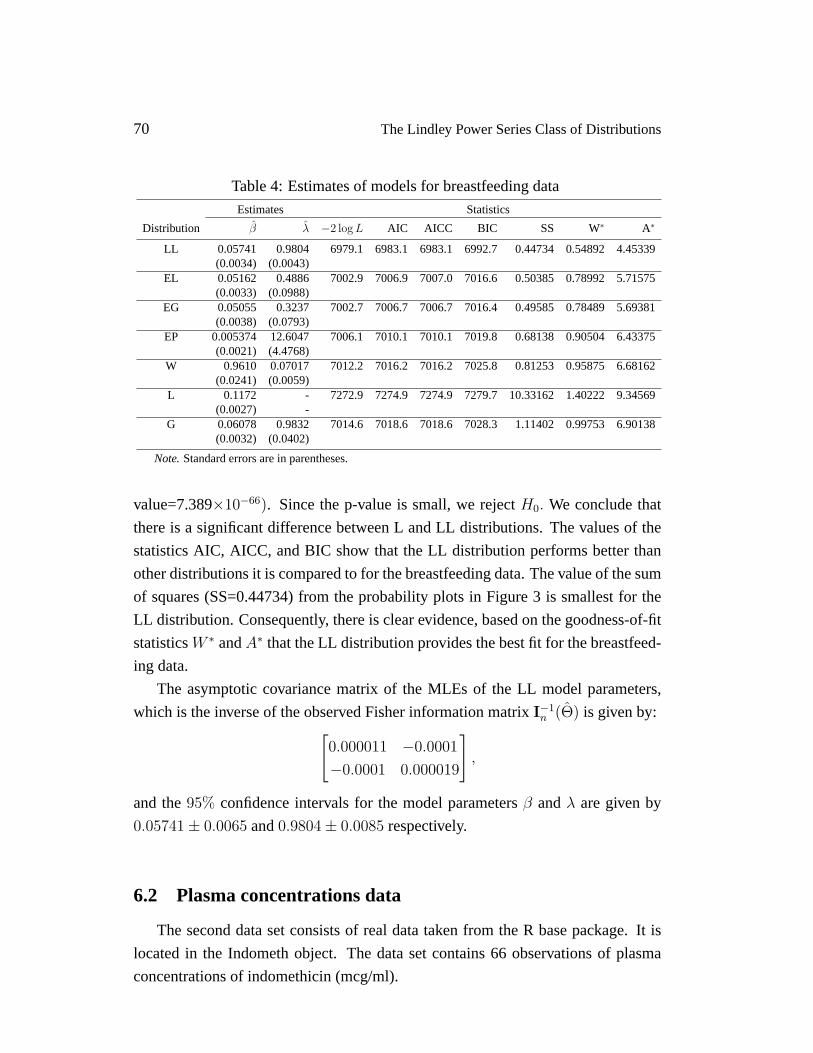
Table 4: Estimates of models for breastfeeding data
Estimates Statistics
Distribution β λ −2 log L AIC AICC BIC SS W∗ A∗
LL 0.05741 0.9804 6979.1 6983.1 6983.1 6992.7 0.44734 0.54892 4.45339(0.0034) (0.0043)
EL 0.05162 0.4886 7002.9 7006.9 7007.0 7016.6 0.50385 0.78992 5.71575(0.0033) (0.0988)
EG 0.05055 0.3237 7002.7 7006.7 7006.7 7016.4 0.49585 0.78489 5.69381(0.0038) (0.0793)
EP 0.005374 12.6047 7006.1 7010.1 7010.1 7019.8 0.68138 0.90504 6.43375(0.0021) (4.4768)
W 0.9610 0.07017 7012.2 7016.2 7016.2 7025.8 0.81253 0.95875 6.68162(0.0241) (0.0059)
L 0.1172 - 7272.9 7274.9 7274.9 7279.7 10.33162 1.40222 9.34569(0.0027) -
G 0.06078 0.9832 7014.6 7018.6 7018.6 7028.3 1.11402 0.99753 6.90138(0.0032) (0.0402)
Note.Standard errors are in parentheses.
value=7.389×10−66). Since the p-value is small, we rejectH0. We conclude that
there is a significant difference between L and LL distributions. The values of the
statistics AIC, AICC, and BIC show that the LL distribution performs better than
other distributions it is compared to for the breastfeeding data. The value of the sum
of squares (SS=0.44734) from the probability plots in Figure 3 is smallest for the
LL distribution. Consequently, there is clear evidence, based on the goodness-of-fit
statisticsW ∗ andA∗ that the LL distribution provides the best fit for the breastfeed-
ing data.
The asymptotic covariance matrix of the MLEs of the LL model parameters,
which is the inverse of the observed Fisher information matrixI−1n (Θ) is given by:[
0.000011 −0.0001
−0.0001 0.000019
],
and the95% confidence intervals for the model parametersβ andλ are given by
0.05741± 0.0065 and0.9804± 0.0085 respectively.
6.2 Plasma concentrations data
The second data set consists of real data taken from the R base package. It is
located in the Indometh object. The data set contains 66 observations of plasma
concentrations of indomethicin (mcg/ml).

Gayan Warahena-Liyanage and Mavis Pararai 71
Figure 3: Histogram, fitted density and probability plots for breastfeeding data
Estimates of the parameters of LL distribution (standard error in parentheses),
Akaike Information Criterion (AIC), Consistent Akaike Information Criterion (AICC),
Bayesian Information Criterion (BIC) are given in Table 5 for plasma concentrations
data. The sum of squares (SS) and the goodness-of-fit statisticsW ∗ andA∗ are also
given.
Plots of the fitted densities and histogram, observed probability versus predicted
probability for the plasma concentrations data are given in Figure 4.
For the hypothesisH0: L againstHa: LL the LR test statistic is 3.4 (p-value
= 0.065196). We conclude that there is no significant differences between L and
LL distributions at the 5% level. However, the result is significant at 10%. The
value of BIC also shows that the L distribution is a better fit, whereas the goodness
of fit-statisticsW ∗ andA∗ show that the LL distribution is better than its sub-model
Lindley (L) distribution and all other distributions that were fitted to the data. The
value of the sum of squares (SS=0.15874) from the probability plots in Figure 4 is
smallest for the LL distribution. Consequently, there is clear evidence, based on the
goodness-of-fit statisticsW ∗ andA∗ that the LL distribution provides the best fit for
the plasma concentration data.
The asymptotic covariance matrix of the MLEs of the LL model parameters,
which is the inverse of the observed Fisher information matrixI−1n (Θ) is given by:[
0.1106 −0.04822
−0.04822 0.03092
],

72 The Lindley Power Series Class of Distributions
Table 5: Estimates of models for plasma concentration data
Estimates Statistics
Distribution β λ −2 log L AIC AICC BIC SS W∗ A∗
LL 1.6572 0.7596 60.9 64.9 65.1 69.3 0.15874 0.23068 1.48439(0.3325) (0.1758)
EL 1.3254 0.3754 61.1 65.1 65.3 69.5 0.15925 0.23235 1.49235(0.3171) (0.2711)
EG 1.2949 0.4080 61.2 65.2 65.4 69.5 0.16284 0.23402 1.50117(0.3691) (0.2598)
EP 1.3178 0.9791 61.4 65.4 65.6 69.7 0.17784 0.23868 1.52920(0.4003) (0.9636)
W 0.9546 1.6857 62.5 66.5 66.7 70.9 0.22627 0.25085 1.60805(0.0904) (0.2078)
L 2.2152 - 64.3 66.3 66.3 68.5 0.36964 0.26346 1.68826(0.2208) -
G 1.6513 0.9773 62.7 66.7 66.9 71.1 0.26865 0.25365 1.62600(0.3257) (0.1495)
Note.Standard errors are in parentheses.
and the95% confidence intervals for the model parametersβ andλ are given by
1.6146± 0.6518 and0.7374± 0.3446 respectively.
6.3 Air conditioning system data
The third data set consists of the number of successive failures for the air condi-
tioning system of each member in a fleet of 13 Boeing 720 jet airplanes. This data
set was used by Proschan [18].
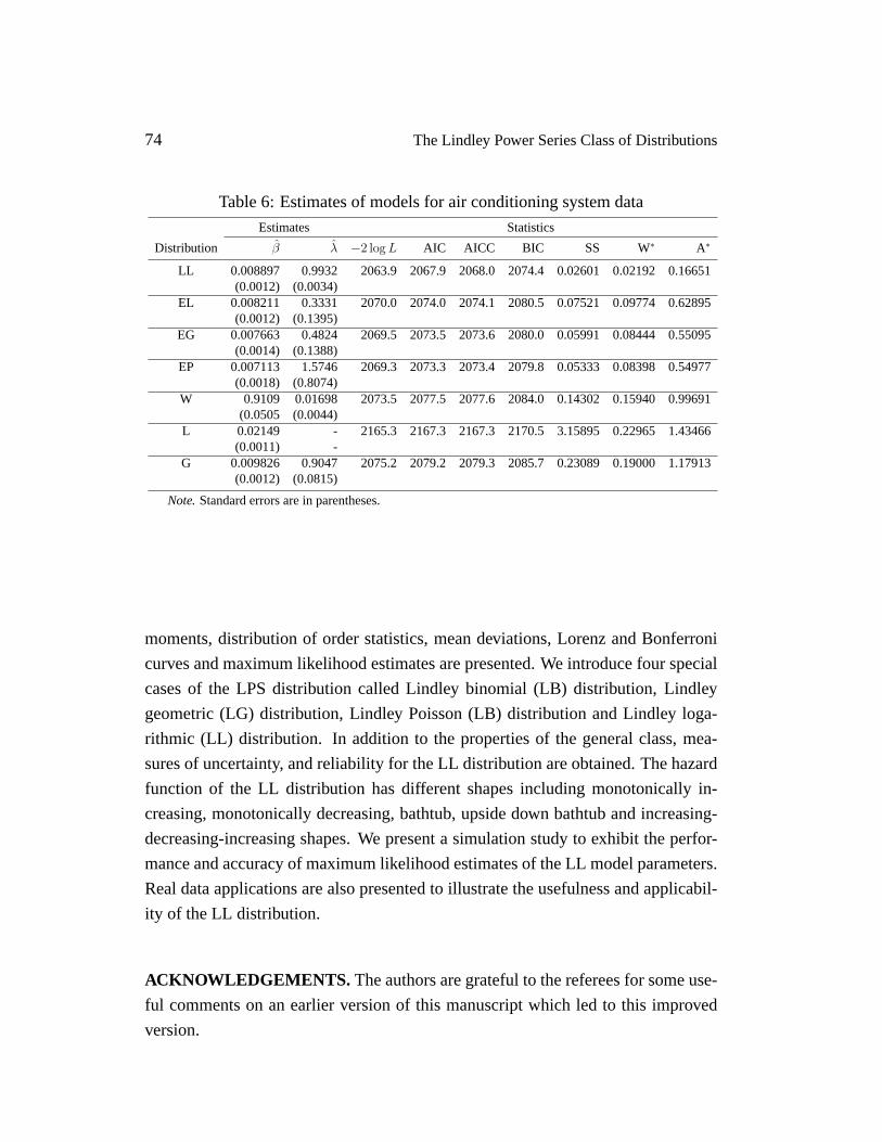
Estimates of the parameters of LL distribution (standard error in parentheses),
Akaike Information Criterion (AIC), Consistent Akaike Information Criterion (AICC),
Bayesian Information Criterion (BIC) are given in Table 6 for the air conditioning
system data. The sum of squares (SS) and the goodness-of-fit statisticsW ∗ andA∗
are also given.
Plots of the fitted densities and histogram, observed probability versus predicted
probability for the air conditioning system data are given in Figure 5.
For the hypothesisH0: L againstHa: LL the LR test statistic is 101.4 (p-
value=7.5163×10⁻²⁴). Since the p-value is small, we reject the null hypothesis.
We can conclude that there is significant difference between the L and LL distribu-
tions. The values of statistics AIC, AICC, and BIC show that the LL distribution
performs the best for the air conditioning data. The value of the sum of squares

Gayan Warahena-Liyanage and Mavis Pararai 73
Figure 4: Histogram, fitted density and probability plots for plasma concentrationsdata
(SS=0.02601) from the probability plots in Figure 5 is smallest for the LL distribu-
tion. Consequently, there is clear evidence, based on the goodness-of-fit statistics
W ∗ andA∗ that the LL distribution provides the best fit for the air conditioning
system data.
The asymptotic covariance matrix of the MLEs of the LL model parameters,
which is the inverse of the observed Fisher information matrixI−1n (Θ) is given by:[
1.459× 10⁻⁶ −3.29× 10⁻⁶
−3.29× 10⁻⁶ 1.1× 10⁻⁵
],
and the95% confidence intervals for the model parametersβ andλ are given by
0.008897± 0.00236 and0.9932± 0.0065 respectively.
7 Concluding Remarks
We propose a new class of lifetime distributions called the Lindley power se-
ries (LPS) class of distributions. This class of distributions is a generalization of
the Lindley (L) distribution and is obtained by compounding the Lindley (L) dis-
tribution and the power series class of distributions. The properties of the LPS
distribution including reverse hazard function, hazard function, quantile function,
74 The Lindley Power Series Class of Distributions
Table 6: Estimates of models for air conditioning system data
Estimates Statistics
Distribution β λ −2 log L AIC AICC BIC SS W∗ A∗
LL 0.008897 0.9932 2063.9 2067.9 2068.0 2074.4 0.02601 0.02192 0.16651(0.0012) (0.0034)
EL 0.008211 0.3331 2070.0 2074.0 2074.1 2080.5 0.07521 0.09774 0.62895(0.0012) (0.1395)
EG 0.007663 0.4824 2069.5 2073.5 2073.6 2080.0 0.05991 0.08444 0.55095(0.0014) (0.1388)
EP 0.007113 1.5746 2069.3 2073.3 2073.4 2079.8 0.05333 0.08398 0.54977(0.0018) (0.8074)
W 0.9109 0.01698 2073.5 2077.5 2077.6 2084.0 0.14302 0.15940 0.99691(0.0505 (0.0044)
L 0.02149 - 2165.3 2167.3 2167.3 2170.5 3.15895 0.22965 1.43466(0.0011) -
G 0.009826 0.9047 2075.2 2079.2 2079.3 2085.7 0.23089 0.19000 1.17913(0.0012) (0.0815)
Note.Standard errors are in parentheses.
moments, distribution of order statistics, mean deviations, Lorenz and Bonferroni
curves and maximum likelihood estimates are presented. We introduce four special
cases of the LPS distribution called Lindley binomial (LB) distribution, Lindley
geometric (LG) distribution, Lindley Poisson (LB) distribution and Lindley loga-
rithmic (LL) distribution. In addition to the properties of the general class, mea-
sures of uncertainty, and reliability for the LL distribution are obtained. The hazard
function of the LL distribution has different shapes including monotonically in-
creasing, monotonically decreasing, bathtub, upside down bathtub and increasing-
decreasing-increasing shapes. We present a simulation study to exhibit the perfor-
mance and accuracy of maximum likelihood estimates of the LL model parameters.
Real data applications are also presented to illustrate the usefulness and applicabil-
ity of the LL distribution.
ACKNOWLEDGEMENTS. The authors are grateful to the referees for some use-
ful comments on an earlier version of this manuscript which led to this improved
version.

Gayan Warahena-Liyanage and Mavis Pararai 75
Figure 5: Histogram, fitted density and probability plots for air conditioning systemdata
References
[1] K. Adamidis and S. Loukas, A lifetime distribution with decreasing failure
rate,Statistics & Probability Letters, 39(1), (1998), 35-42.
[2] W. Barreto-Souza, A.L. de Morais and G.M. Cordeiro, The Weibull-geometric
distribution,Journal of Statistical Computation and Simulation, 81(5), (2011),
645-657.
[3] H. Bidram and V. Nekoukhou, Double bounded Kumaraswamy-power series
class of distributions,SORT-Statistics and Operations Research Transactions,
1(2), (2013), 211-230.
[4] R.M. Corless, G.H. Gonnet, D.E. Hare, D.J. Jeffrey and D.E. Knuth, On the
LambertW function,Advances in Computational Mathematics, 5(1), (1996),
329-359.
[5] M.E. Ghitany, D.K. Al-Mutairi, N. Balakrishnan and L.J. Al-Enezi, Power
Lindley distribution and associated inference,Computational Statistics &
Data Analysis, 64, (2013), 20-33.
[6] M.E. Ghitany, B. Atieh and S. Nadarajah, Lindley distribution and its applica-
tion, Mathematics & Computers in Simulation, 78(4), (2008), 493-506.
76 The Lindley Power Series Class of Distributions
[7] W. Gui, S. Zhang and X. Lu, The Lindley-Poisson distribution in lifetime
analysis and its properties,Journal of Mathematics & Statistics, (2014), 10-
63.
[8] N.L. Johnson, A.W. Kemp and S. Kotz,Univariate discrete distributions, John
Wiley & Sons, 2005.
[9] J.P. Klein and M.L. Moeschberger,Survival analysis: techniques for censored
and truncated data, Springer Science & Business Media, 2003.
[10] C. Kus, A new lifetime distribution,Computational Statistics & Data Analysis,
51(9), (2007), 4497-4509.
[11] D.V. Lindley, Fiducial distributions and Bayes’ theorem,Journal of the Royal
Statistical Society, Series B (Methodological), (1958), 102-107.
[12] W. Lu and D. Shi, A new compounding life distribution: the Weibull Poisson
distribution,Journal of Applied Statistics, 39(1), (2012), 21-38.
[13] E. Mahmoudi and A.A. Jafari, Generalized exponential power series distribu-
tions,Computational Statistics & Data Analysis, 56(12), (2012), 4047-4066.
[14] E. Mahmoudi and A.A. Jafari, The Compound Class of Linear Failure
Rate-Power Series Distributions: Model, Properties and Applications, arXiv
preprint arXiv:1402.5282, (2014).
[15] A.L. Morais and W. Barreto-Souza, A compound class of Weibull and power
series distributions,Computational Statistics & Data Analysis, 55(3), (2011),
1410-1425.
[16] A. Noack, A class of random variables with discrete distributions,The Annals
of Mathematical Statistics, (1950), 127-132.
[17] M. Pararai, G. Warahena-Liyanage and B.O. Oluyede, Exponentiated Power
Lindley Poisson Distribution: Properties and Applications, Submitted toCom-
munications in Statistics-Theory and Methods, (2015).
[18] F. Proschan, Theoretical explanation of observed decreasing failure rate,Tech-
nometrics, 5(3), (1963), 375-383.

Gayan Warahena-Liyanage and Mavis Pararai 77
[19] A.L.F.R.P.E.D. Renyi, On measures of entropy and information,In Fourth
Berkeley Symposium on Mathematical Statistics & Probability, 1, (1961), 547-
561.
[20] E.A. Shannon, A Mathematical Theory of Communication,The Bell System
Technical Journal, 27(10), (1948), 461-464.
[21] E.A. Shannon, A Mathematical Theory of Communication,The Bell System
Technical Journal, 27(10), (1948), 379-423.
[22] R. Tahmasbi and S. Rezaei, A two-parameter lifetime distribution with de-
creasing failure rate,Computational Statistics & Data Analysis, 52(8), (2008),
3889-3901.
[23] G. Warahena-Liyanage and M. Pararai, A Generalized Power Lindley Dis-
tribution with Applications,Asian Journal of Mathematics and Applications,
2014, Article ID ama0169, (2014), 1-23.
[24] H. Zakerzadeh and E. Mahmoudi, A new two parameter lifetime distribution:
model and properties, arXiv preprint arXiv:1204.4248, (2012).

78 The Lindley Power Series Class of Distributions
R Algorithms
In this appendix, we present R codes to compute cdf, pdf, moments, reliability,
Renyi entropy, mean deviations, maximum likelihood estimates and variance-covariance
matrix for the LL distribution.

Gayan Warahena-Liyanage and Mavis Pararai 79

80 The Lindley Power Series Class of Distributions


