
IJRRAS 25 (3) ● December 2015 www.arpapress.com/Volumes/Vol25Issue3/IJRRAS_25_3_05.pdf
82
THE MEASUREMENT OF THE DIELECTRIC CONSTANT OF THREE
DIFFERENT SHAPES OF CONCRETE BLOCKS
David McGraw Jr.,
University of Louisiana at Monroe
E-mail address: [email protected]
ABSTRACT
To optimize the effectiveness of the rehabilitation of underground utilities, taking in consideration limitation of
available resources, there is a need for a cost effective and efficient sensing systems capable of providing effective, in
real time and in situ, measurement of infrastructural characteristics. To carry out accurate non-destructive condition
assessment of buried and above ground infrastructure such as sewers, bridges, pavements and dams, advanced ultra-
wideband (UWB) based radar was developed at Louisiana Tech University (LTU). One of the major issues in
designing the FCC compliant UWB radar was the contribution of the pipe wall, presence of complex soil types and
moderate-to-high moisture levels on penetration depth of the electromagnetic (EM) energy.
The electrical properties of the materials involved in designing the UWB radar exhibit a significant variation as a
result of the moisture content, mineral content, bulk density, temperature and frequency of the electromagnetic signal
propagating through it. In this paper, the dielectric constant of concrete blocks is measured over a microwave
frequency range from 1 Ghz to 18 Ghz including the effects of moisture and chloride content. A high performance
software package called MU-EPSLNTM was used for the calculations. Data reduction routines to calculate the complex
permeability and permittivity of materials as well as other parameters are also provided. The results obtained in this
work will be used to improve the accuracy of the numerical simulations and the performances of the UWB radar
system.
1. INTRODUCTION
Of the approximately 11 million miles of underground utilities in the U.S, potable, storm and wastewater distribution
and collection systems make nearly 6.2 million miles. Efficient operation of such a system is essential in maintaining
basic societal needs which includes public health and environmental protection. Still, due to the costs associated with
their maintenance, underground utilities are suffering from increasing rates of failure. Report released by Battelle
Memorial Institute [1] estimated annual expenditures on water work rehabilitation in the U.S. at 4.5 billion dollars,
with an annual projected grow of 8% to 10%.
To optimize the effectiveness of the rehabilitation of underground utilities, taking in consideration limitation of
available resources, there is a need for a cost effective and efficient sensing systems capable of providing effective, in
real time and in situ, measurement of infrastructural characteristics. As an example, development of advanced
technologies for condition assessment of civil infrastructure systems was considered by the National Institute for
Standards and Technology (NIST) a “critical national need” [2]. To carry out accurate non-destructive condition assessment of buried and above ground infrastructure such as sewers,
bridges, pavements, dams, walls, and foundations, an advanced ultra-wideband (UWB) based radar was developed at
Trenchless Technology Centre (TTC) and Centre for Applied Physics Studies (CAPS) at Louisiana Tech University
(LTU). A significant contribution in the process of designing such an ultra-wideband (UWB) based radar system came
from a two- and three-dimensional numerical modeling of the propagation of electromagnetic pulses inside and outside
buried non-metallic pipes using the finite difference time domain (FDTD) technique [3]. To satisfy the Federal
Communication Commission (FCC) imposed limits on the electromagnetic emissions for UWB imaging systems the
condition assessment radar was designed at Louisiana Tech University to operate in the bandwidth of 3.1 to 10.6 GHz.
The electrical properties of the materials involved in designing the UWB radar exhibit a significant variation as a
result of the moisture content, mineral content, bulk density, temperature and frequency of the electromagnetic signal
propagating through it. The measurement of the complex dielectric is important in many areas of research. Dielectric
measurements are important in this research, because it can provide the electric or magnetic characteristics of
materials. There is a growing industrial demand for dielectric characterization of materials for design, manufacturing,
and quality control purposes in industries [4]. This research measures the dielectric properties of materials using a
coaxial line fixture. A method for determining the dielectric constant of three different shapes of concrete blocks will
be described in this research. A high performance software package called MU-EPSLNTM has been used to do the
calculations. The MU-EPSLNTM is a complete software package for making S-parameter measurements using one and
two port coax or waveguide fixtures. Data reduction routines to calculate the complex permeability and permittivity
of materials as well as other parameters are provided. The user has access to all raw and processed data, so that it can

IJRRAS 25 (3) ● December 2015 McGraw ● The Measurement of the Dielectric Constant
83
be studied at any time. The user can select bands to be swept; many frequencies can be swept depending on the VNA.
All the capabilities of the VNA are available to the user either through the external controller or the front panel [5].
The complex µ and є are normalized relative to free space parameters µ0 and є0.
The complex µ and є are written as
µ = µ’ – i µ” (1.1)
є = є’ – i є” (1.2)
where µ” and є” are nonnegative real numbers and i = 1 . The complex time dependence in the relevant field
equations is of the form ejωt. The MU-EPSLNTM program calculates the free space and short backed reflection and
transmission coefficients for a material. The sample thickness is input by the user. This implementation is based upon
a direct analogy of TEM propagation in a coaxial line, and a normally incident plane wave propagation in a coaxial
line, and a normally incident plane wave propagating in free space. A measurement that uses the
Transmission/Reflection line technique involves putting a sample in a section of a coaxial line, and measuring the two
ports complex scattering parameters with a vector network analyzer (VNA). The VNA must be calibrated before a
measurement can be made.
The Transmission/Reflection line technique involves the need to measure both reflected (S11) and transmitted (S21).
The relevant scattering parameters relate closely to the complex permittivity and permeability of the material by
equations. The conversion of s-parameter to complex dielectric parameter is computed by solving the equations using
a computer program. The different samples were machined to fit into the sample holder [6]. Calibrations in
transmission line measurements use different terminations that produce various resonant behaviors in the transmission
line.
For good dielectric measurement, a high electric field is required. This measurement technique allows for the
measurement of permittivity and permeability of the dielectric material. The VNA can be calibrated and the samples
are then placed in the sample holder. The better that the sample fits the less the measurement uncertainty will be. The
measurement accuracy is limited by the numerical uncertainty and by the air gaps [7]. Cylindrical samples specimens
were made using a drill press. The specimens were drilled from different types of concrete blocks. Dimensions of the
specimens varied from two to three cm in diameter to four to five cm in height.
A number of different conditions of the specimens were used for the measurements: (1) saturated specimens with
moisture on the inside for one month or more, (2) air dried specimens exposed to just room temperature and humidity,
and finally (3) specimens were placed into saltwater for one month or more. Concrete is a dielectric, nonmagnetic
material. Dielectric materials are usually made up of atoms whose valence electron shells are nearly full, resulting in
low conductivity. Using a coaxial transmission line, a particular material’s dielectric properties can be tested as
amounts of certain substances within it are varied. For concrete, there have been studies to ascertain the effects of
different admixtures, the type of aggregate, water content, and curing time on dielectric properties [8].
In general, the real part of the dielectric constant is larger when it is easier for the material to polarize, meaning that
the ions are mobile and there is little crystallization. The addition of chlorides increases the dielectric constant, as does
the amount of water. The dielectric constant decreases over curing time, because the amount of water decreases during
this time. Also, the dielectric constant of concrete is dependent on the constant of its aggregate: mixes containing
limestone have a higher constant than those containing granite, this correlates with the fact that limestone itself has a
higher constant than granite does [9].
There are certain concrete properties that influence the performance of concrete blocks. These properties include
concrete compressive strength, density, absorption, water cement ratio, cement content and type, and aggregates. All
of these factors would have an influence on the dielectric properties of concrete blocks. For example, the dielectric
constant for concrete with coarse aggregates is higher than concrete with fine aggregates. Concrete strength is a
function of many factors including, aggregates, cement material, manufacturing, curing process, and mix design.
These factors must also play a role in the dielectric constant of concrete blocks, since the concrete blocks’ strength is
a function of these same factors. Concrete blocks design strengths refer to 28 days concrete strengths, but in actuality,
the design strengths are obtained much earlier than 28 days. Quality concrete block densities typically range from
145-155 pounds per cubic foot. In general, the higher the density of concrete block, the greater the durability of the
concrete, which leads us to believe that the dielectric constant could be affected by, changes in density.
Absorption is primarily used to check the density of the concrete. As with compressive strength, the absorption can
be greatly influenced by the aggregates and the manufacturing process that is used for each concrete blocks. The key
to proper cement content is proper design of the mix, with consideration of all material properties, manufacturing, and
curing processes. Materials used to manufacture concrete blocks consist of aggregates and manufactured products,
such as Portland cement and reinforcing steel. Each of the components has a standard specifying its properties and
methods of testing. Portland cement is a closely controlled chemical combination of calcium, silicon, aluminum, iron,

IJRRAS 25 (3) ● December 2015 McGraw ● The Measurement of the Dielectric Constant
84
and small amounts of other compounds. Gypsum, which regulates the setting time of the concrete, is added during the
final process of grinding.
Calculating the dielectric constant of a mult-phased heterogeneous composite like concrete is a challenging task.
Chemical admixtures are also used in practice as a processing addition to aid in manufacturing and handling of
concrete or as a functional addition to modify the properties of concrete. In this research, the problems of chemical
admixtures or the microscopic structure in calculating the dielectric constant are not considered [10].
2. LITERATURE REVIEW
Concrete is one of the world’s most commonly used building materials. The basic form of concrete is a mixture of
paste and aggregates. The material paste used to manufacture concrete blocks is cement, fine aggregate and coarse
aggregate. A concrete block is generally used as a building material in the construction of walls, and foundations. A
concrete blocks is one of several precast concrete products used in construction. The term precast means that the
blocks are formed and hardened before they are brought to the job site. Most concrete blocks have one or more hollow
cavities, and their sides may be cast smooth or with a design. There is a need to understand concrete blocks as a
material, because of growing concern about the deterioration of the worldwide infrastructures. It is therefore important
to understand the electromagnetic properties of concrete blocks in general. Concrete is made by adding water to a
mixture of cement, sand, and coarse aggregate. Hydration takes place between the water and cement producing a
matrix of compounds known as cement paste. This matrix locks together the coarse and fine aggregate particles to
form a material with considerable compressive strength. A concrete mix is normally defined by the mass ratios of its
constituents, i.e.: the water/cement ratio, the cement/sand/aggregate ratio and the cement/total-aggregate ratio. The
real and imaginary parts of the complex permittivity of different concrete mixes have been investigated by a number
of different authors [11][12]. Data presented by Shah, Hasted and Moore refer mostly to the real and imaginary parts
of the complex permittivity of hardened concrete. These data characterize the complex permittivity for different water-
cement ratios, for conditions of different water volume absorption. Results were recorded at 3 GHz, 9 GHz, and 24
GHz [13]. For the interesting case where concrete can be considered dry or having a small amount of water content,
the real part of the complex permittivity was found to vary between 5.0-7.0 while the imaginary part between 0.1-0.7.
Data was also recorded for aerated concrete at 3.0 GHz and 9.0 GHz [13]. Aerated concrete consists of a cement paste
to which a small proportion of aluminum powder is added. During the heating process the aluminum is oxidized
producing sufficient hydrogen to aerate the mix into a strong light material. In this case and for small water contents,
the real part of the complex permittivity was found to vary between 2.0-2.5, while the imaginary part was between
0.12-0.50. All the constitutive parameters presented up to now for different concrete types, do not vary significantly
from data recorded by other sources. In the latter case for the range of frequencies 1- 95.9 GHz the real part of the
complex permittivity was found to vary from 6.0-7.0 and the imaginary part was found to vary from 0.34 to 0.85 for
hardened concrete. In [13], aerated concrete measured at 1GHz was found to have a value of εcomplex = 2 – i0.5 which
is close to the values reported at 3.0 GHz and 9.0 GHz. Similar measurements between 0.5-0.7 GHz suggest a value
for the relative permittivity between 2.5-3 and a conductivity range between 0.0138-0.025 (S/m) [13].
An open-ended coaxial probe method was used by Buyukozturk and Rhim to measure real and imaginary parts of the
complex permittivity of hardened concrete [14]. They looked at the frequency range of 0.1 to 20 GHz at 0.4 GHz
steps. Also, they used different moisture content to examine the effects of moisture on the electromagnetic properties
of concrete. They used cylindrical concrete samples that were casted with a water/cement/sand/coarse aggregate mix.
Portland cement of Type 1 was used. It appears that at dry conditions, the dielectric constant does not very much over
the measured frequency range. This is not true when the moisture level increases. The dielectric constant of the
saturated sample is almost double that of the oven dried sample. This is possible due to the high value of the dielectric
constant of water [15]. So then, the increases of water content in concrete must greatly affect the change in the
dielectric constant of the concrete.
A co-axial transmission line test rig was used by Stoutsos and associates in 2001, to measure the dielectric properties
of concrete. Measurements were made on nineteen samples at various levels of water volume as a percentage of
concrete. All samples were made using ordinary Portland cement and the concrete mixes were made with ten mm
gravel aggregate with Hope Quarry sand. They provided measurements data showing the variation of permittivity and
conductivity with frequency and moisture content. The values that they measured were in the range of previous studies
with the dielectric constant of dry concrete between 3.5 and 5.0[15]. In 2006, Rohde and Schwarz performed a similar
measurement on five samples of concrete, but they used the maximum size of 30 mm gravel aggregate. The data
showing the influence of moisture content and the effects of chloride on the permittivity were presented [16].
Five material models with frequency-dependent permittivity were compared to the experimental data. Kaatze,
compared two models, the Cole-Cole model and the Debye’s model; he thought the Cole-Cole model worked the best
in fitting the measurement values [17]. In the literature, several techniques have been used to extract permittivity and
permeability of materials. For example, the rectangular waveguide technique is one of a class of two ports

IJRRAS 25 (3) ● December 2015 McGraw ● The Measurement of the Dielectric Constant
85
measurement which includes transmission and refection. It has been used as an easy way for studying properties of
materials in the microwave frequency. The results of these studies obtain results which are very similar [17]. They
measured the complex permittivity for concrete, based on measuring the scattering parameters.
Belrhiti, Bri, Nakheli, Haddad, and Mamouni presented their results of studying the dielectric constant of concrete
using Ku band [18]. They measured the dielectric constant using a Vector Network Analyzer using a thru-reflect-line
calibration. The Newton-Raphson method was used as a numerical tool to estimate the value of relative complex
permittivity. The results that they obtained were compared with the Nicholson-Ross technique. The two methods were
in good agreement [18]. The researchers who have studied the dielectric constant of concrete have stated that the
complex permittivity of concrete samples does not vary significantly due to frequency changes, even over a wide
frequency range. It does not change significantly for different mixing ratios of similar materials. It seems that the
biggest difference observed is between hardened and lightweight, aerated concrete samples. The concrete parameters
presented up to now referred to non-reinforced concrete samples.
In the case of reinforced concrete, it has been shown that other parameters that can influence the transmission
characteristics of a concrete wall include the square grid side length and the steel diameter used in the reinforced
concrete. Even in these cases, the value of the complex permittivity used to describe the concrete was equal to εcomplex
= 7 – i0.3 for 900 MHz and 1800 MHz [19]. The following table summarizes the dielectric constant data on concrete.
Table 2-1. Dielectric Constant Data For Concrete.
Concrete Dry
relative
dielectric
constant
Complex dielectric
constant
WET
Relative
dielectric
constant
SALTWATER
Relative
Dielectric
constant
Below 5 Ghz 2.5 to 7 0.1 to 0.7 8 to 12 8 to 12
Below 20 Ghz 2.5 to 7 0.1 to 0.7 8 to 12 8 to 12
Below 95 Ghz 2.5 to 7 0.0138 to 0.025 8 to 12 8 to 12
3. THEORY
Materials can be characterized by electric permittivity ε, electric conductivity σ, magnetic permeability μ, and
magnetic conductivity σ*. The frequency-dependence of all these properties is termed dielectric dispersion. We can
assume concrete to be as a homogeneous, isotropic, and lossless dielectric medium, although this is not totally the
case. Dielectric properties of a material can be used to determine other material properties such as moisture content,
and bulk density [20]. This section provides the background information regarding the theory of dielectric properties
of materials in general. Dielectric properties can be interpreted both microscopically and macroscopically.
Microscopically, dielectric properties represent the polarization ability of molecules in the material corresponding to
an externally applied electric field. Macroscopically, dielectric properties are the relationship between the applied
electric field strength E* and the electric displacement D,* both externally measured. Dielectric properties are the
collective terms of electric permittivity ε, electric conductivity σ, magnetic permeability μ, and magnetic conductivity
σ.*
IJRRAS 25 (3) ● December 2015 www.arpapress.com/Volumes/Vol25Issue3/IJRRAS_25_3_05.pdf
86
Materials are described and classified by these properties into various types, such as metals and dielectrics [20]. Our
research is with concrete blocks, so the study will consider only isotropic materials. All of the properties of isotropic
materials are described by first-order tensors. These quantities can be real or complex, depending on the nature of the
material. When electric fields are applied to concrete blocks, the quantities are generally complex. Complex electrical
permittivity ε (F/m) describes the ability of a material to interact with an applied electric field. It is defined as the ratio
between the electric displacement D* (C/m2) and the electric field E*(V/m). Generally,
�⃗⃗� * = ε �⃗� * (3.1)
where ε = ε ( ) for dielectric materials. It represents the ability of a material to permit an electric field to pass through
the material [20]. For dielectric materials their frequency-dependent response is subject to applied electric fields,
which is the result of the molecular polarizability. Their delayed and attenuated response is also observed and
described as the dielectric dispersion phenomenon attributing to several polarization phenomena in the microscopic
level. To account for these absorption and losses an imaginary part is needed in the dielectric description of the material
property [20]. Therefore, the complex electrical permittivity (or complex permittivity) is defined as
ε = ε’ + i(-ε”) = ε’ – iε” (3.2)
where ε’ is the real part of ε representing the ability of a material to store energy that is carried by the electromagnetic
field transmitting through it, and ε” is the imaginary part representing energy absorption and loss. The negative sign
defines ε” as applied since energy dissipation/loss occurs to the concrete blocks in our research. A positive sign of ε”
would suggest that energy is being created. The measured values of ε’ and ε” mainly depend on measured frequency
and temperature, while in some cases, as well as pressure [20]. For example, the Debye equations provide a frequency-
dependent representation of ε’ and ε”, satisfying the Kramers-Kronig relations, as
ε’ ( ) = εi+ εs – εi / (1 + ( )2) (3.3)
ε”( ) = (εs – εi)/ (1 + ( )2) (3.4)
where = 2 f is the angular frequency, f is the temperal frequency, εi is the permittivity measured by electric (ac)
current field at frequency = , εs is the permittivity measured by the electric (dc) current field at frequency = 0,
and is the characteristic relaxation time [38]. The relaxation time is usually represented by,
t = /2 . (3.5)
Materials whose response can be described by the Debye equations are called Debye material.
We find Kramers-Kronig relations by using Fourier Transforms. We begin with the relation between the electric field
and displacement at some particular frequency .
�⃗⃗� (x, ) = ε ( ) �⃗� (x, ) (3.6)
where we note the two Fourier transform relations:
�⃗⃗� (x, t) = 1
√2𝜋
D
(x, ) e-i t d (3.7)
�⃗⃗� (x, ) = 1
√2𝜋
D
(x, t’) ei t’dt’ (3.8)
and also, we have:
�⃗� (x, t) = 1
√2𝜋E
(x, ) e-i t d (3.9)
�⃗� (x, ) =1
√2𝜋
E
(x, t’) ei t dt’ (3.10)
Therefore:
�⃗⃗� (x, t) = 1
√2𝜋
( ) e-i t d
1
√2𝜋
E
(x, t’) ei t’ dt’ (3.11)
�⃗⃗� (x, t) = ε0 { �⃗� (x, t)
G (τ) �⃗� (x, t – τ) dτ } (3.12)
where I have introduced the susceptibility kernel:
IJRRAS 25 (3) ● December 2015 McGraw ● The Measurement of the Dielectric Constant
87
G(τ) = 1
√2𝜋
(𝜀(𝜔)
(𝜀0)− 1)e-i t d (3.13)
G(τ) = 1
√2𝜋
0( ) e-i t d (3.14)
where ε ( ) = ε0 (1 + 0( )). This equation is nonlocal in time unless G(𝜏) is a delta function, which in turn is true
only if the dispersion is constant [20]. To understand this consider the susceptibility kernel for a simple one resonance
model. In this case we have
0 = ε/ε0 – 1 = p2/ ( 0
2 - 2 – i 0 ) (3.15)
then,
G (τ) = 𝜔𝑝
2
2𝜋∫
1
(𝜔02− 𝜔2−𝑖𝛾0𝜔)
∞
−∞e- i τ d (3.16)
This is an integral we can do using contour integration methods. We use the quadratic formula to find the roots of the
denominator, and then write the factored denominator in terms of the roots:
1, 2 = -i √−𝛾2 + 4𝜔02 / 2 (3.17)
1,2 =( -i / (2 ± 𝜔0√1 − 𝑢 ) (3.18)
where u= 2
0
2 4/ and 0 0 as long as 0 >> /2. Then,
G(τ) = (2 i) 𝜔𝑝
2
2𝜋 c [1
(𝜔− 𝜔1)(𝜔−𝜔2)] e -i τ d (3.19)
If we close the contour in the upper half plane, we have to restrict τ < 0, because otherwise the integrand will
not vanish on the contour at infinity where the positive imaginary part has. If we close the integrand in the lower
half plane, τ > 0 and we have:
G(τ) = p2 e- 2/ sin ( 0)/ 0 (τ) (3.20)
where this is a function to enforce the τ > 0 constraint. Then we can use complex variables and Cauchy’s theorem to
continue to solve the problem [20]. We start by noting that G (τ) is real, and then we get: 𝜀(𝜔)
𝜀0 − 1= iG(0)/ - G’(0)/ 2 + ….. (3.21)
from which we can conclude that ε(- ) = ε*( *). Note the even/odd imaginary/real in the series, and ε( ) is
therefore analytic in the upper half plane and so we have:
𝜀(𝑧)
𝜀0 -1=
1
2𝜋𝑖 c 𝜀(𝜔′)
(𝜀0−1)(𝜔′−𝑧)d ’ (3.22)
If we let z = + i , then we have:
1/ ( ’ - - i ) = P [1/ ( ’ - )] + i ( ’ - ) (3.23)
If we substitute this into the integral above along the real axis only, we have:
𝜀(𝜔)
𝜀0 = 1 +
1
𝑖𝜋𝑃
𝜀(𝜔′)
(𝜀0−1)(𝜔′− 𝜔) d ’ (3.24)
Although this looks like a single integral, because of the i in the denominator it is really two integrals. The real part
of the integrand becomes the imaginary part of the result and vice versa. So what we have this is:
𝑅𝑒(𝜀(𝜔)
𝜀0) = 1 +
1
𝑖𝜋𝑃
Im
𝜀(𝜔′)
𝜀0( 𝜔′− 𝜔) d ’ (3.25)
𝐼𝑚(𝜀(𝜔)
𝜀0) = -
1
𝜋 P
Re
𝜀(𝜔′)
(𝜀0−1)(𝜔′− 𝜔) d ’ (3.26)
These are the equations that we know as the Kramers-Kronig relations [21]. A dimensionless representation is also
used for defining the complex permittivity. The complex relative permittivity is defined by
εr = ε /ε0 = (ε’ – iε”) / ε0 = ε’r – iε”r (3.27)
where ε0 is the electrical permittivity of free space, ε’r is the dimensionless dielectric constant, and ε”r is the
dimensionless loss factor. It is only the dimensionless nature leading to the name “dielectric constant” since ε’r is not
a constant when considered over a range of frequencies [22]. The ratio between ε’r and ε”r is the loss tangent or
dissipation factor, so when have:
tan = ε”r / ε’r = ε” / ε’ (3.28)

IJRRAS 25 (3) ● December 2015 McGraw ● The Measurement of the Dielectric Constant
88
This dimensionless representation (ε / ε0 , tan ) is simpler then and has an advantage over the original (ε’ , ε”)
representation because it clearly shows that the material is different from free space. Complex magnetic permeability
describes the ability of a material to interact with an applied magnetic field. It is the ratio between the magnetic
field flux density B and the magnetic field H.
�⃗� = �⃗⃗� (3.29)
is a scalar for isotropic materials. The complex magnetic permeability is used when magnetic losses are present in
the material [23][24].
= ’ – i ” (3.30)
where ’ and ” are the real and imaginary parts of the complex permeability. The negative imaginary part of
suggests the energy dissipation. A dimensionless relative complex permeability can be further defined as
r = ’ – i ”/ 0 = ’r - i ”r (3.31)
where 0 is the permeability of free space. Definitions of various materials are listed in Table 3-1.
Table 3-1: Types of magnetic materials
Description Criterion
Feromagnetic r > 10
Paramagnetic 1 < r < 10
Diamagnetic r < 1
Non-magnetic r = ’r = 1, ”r = 0
Apparent electrical permittivity εa is defined by accounting for the direct current conductivity loss in the representation
of complex permittivity. Since the imaginary part transmitting through the material [24].The total energy dissipation
in the material can be expressed by the dissipated or absorbed power using the complex poynting vector theorem and
the Maxwell’s equations. When dealing with electromagnetic fields a way is needed to relate the concept of energy to
the fields [50]. This is done by means of the Poynting vector:
�⃗� = �⃗� х �⃗⃗� (3.32)
where E is the electric field intensity, H is the magnetic field intensity, and P is the Poynting vector. The absolute
value of Poynting vector is found to be the power density in an electromagnetic field. By using the Maxwell’s
equations for the curl of the fields along Gauss’s divergence theorem and an identity from vector analysis, we may
prove what is known as the Poynting theorem. The Maxwell’s equations needed are
х �⃗� = - ∂�⃗� / ∂t (3.33)
х �⃗⃗� = 𝐽 + ∂�⃗⃗� / ∂t (3.34)
along with the material relationships:
�⃗⃗� = ε0�⃗� + �⃗� (3.35)
�⃗� = 0�⃗⃗� + 0�⃗⃗� (3.36)
or for isotropic materials
�⃗⃗� = ε�⃗� (3.37)
�⃗� = �⃗⃗� (3.38)
In addition, the identity from vector analysis,
•(�⃗� х �⃗⃗� ) = - �⃗� • ( х �⃗⃗� ) + �⃗⃗� • ( х �⃗� ) (3.39)
Is needed. If PA is to be the power density, then its surface integral over the surface of a volume must be the power
out of the volume. So next do the negative of the surface integral to obtain P, the power into the volume:
�⃗� 𝐴= - �⃗� х �⃗⃗� • 𝑑𝑆⃗⃗⃗⃗ . (3.40)

IJRRAS 25 (3) ● December 2015 McGraw ● The Measurement of the Dielectric Constant
89
Now we can use Gauss’s divergence theorem on the integral in equation (3.42), along with equation (3.41) , we have:
�⃗� 𝐴 = - (�⃗� х 𝐻)⃗⃗⃗⃗ ⃗ • 𝑑𝑆⃗⃗⃗⃗
�⃗� 𝐴 = - • (�⃗� х �⃗⃗� ) dV
�⃗� 𝐴 = �⃗� • ( х �⃗⃗� ) + �⃗⃗� • (- х �⃗� ) dV (3.41)
Next, substituting from Maxwell’s equations, we can obtain:
�⃗� 𝐴= - �⃗� х �⃗⃗� • 𝑑𝑆⃗⃗⃗⃗ = �⃗� • 𝐽 dV + �⃗� • ∂�⃗⃗� /∂t dV + �⃗⃗� • 𝜕𝐵⃗⃗⃗⃗ ⃗/∂t dV (3.42)
Equation (3.42) is the Poynting theorem. The complex Poynting vector p is
�⃗� = ½ s
(�⃗� х �⃗⃗� *) dS (3.43)
where S is a closed surface and dS is a vector element of area directed outward from the volume V, H* is the conjugate
of the magnetic field H. The divergence theorem provides
s
(�⃗� х �⃗⃗� *)dS = v
•( �⃗� х �⃗⃗� *) dV. (3.44)
From vector calculus we have
• (𝐸⃗⃗⃗⃗ х 𝐻)⃗⃗⃗⃗ ⃗ = ( х �⃗� ) • �⃗⃗� * - ( х �⃗⃗� *) • �⃗� (3.45)
with Maxwell’s equations х �⃗� = i �⃗� and х �⃗⃗� = i �⃗⃗� + 𝐽 , Ohm’s law 𝐽 = σ • �⃗� , and �⃗� = μ�⃗⃗� , the complex
Poynting vector becomes
½ s
(�⃗� х �⃗⃗� *) d𝑆 = ½ V
[(- i μ • �⃗⃗� ) • �⃗⃗� * + (i ε • �⃗� – σ • �⃗� )]dV. (3.46)
If we rearrange our equations, then
Re[ ½ s
(�⃗� х �⃗⃗� *)(-d𝑆 )] = /2 v
(μ”�⃗⃗� •�⃗⃗� * + ε” 𝐸 ⃗⃗ ⃗• �⃗� * + σ/ �⃗� •�⃗� *) dV (3.47)
Im [ ½ s
(�⃗� х �⃗⃗� *) (-d𝑆 )] = /2 v
(μ’�⃗⃗� • �⃗⃗� * - ε’ �⃗� • �⃗� *) dV (3.48)
where - dS is the vector pointing toward the closed surface S and tangent to the surface boundary [24]. The real part
of the complex Poynting vector is the dissipated energy Pdis absorbed by the material, which consists of three parts;
magnetic loss, electric loss, and conductivity loss.
Since μ” = 0 for non-magnetic materials, Pdis becomes
�⃗� dis = /2 v
(ε” + σ/ ) �⃗� • �⃗� * dV = / 2 v
ε �⃗� •�⃗� * dV (3.49)
and the effective dielectric loss factor is
ε”e = ε” + σ/ (3.50)
So then we can write an effective conductivity which is defined as
e = ε”e = ε” + σ (3.51)
where σ = σs is the electrical conductivity measured at the static frequency ( = 0). This conductivity is the real part
of the complex conductivity [52]. So now that we know the effective dielectric loss factor, we can define the apparent
complex permittivity as
εa = ε” – iε”e = ε’ – i(ε” + σs/ ) (3.52)
Definitions of materials based on our apparent complex permittivity are listed in Table 3-2.
IJRRAS 25 (3) ● December 2015 McGraw ● The Measurement of the Dielectric Constant
90
Table 3-2: Types of dielectric materials
Description Criterion
Perfect Dielectric ε” > 0, ε”e = 0
Imperfect Dielectric ε’ > 0 , ε”e > 0
Complex electrical conductivity σ describes the ability of a material to conduct an applied electric current, represented
by the ratio between the electric current density 𝐽 and the electric field 𝐸.
𝐽 = σ • �⃗� (3.53)
where σ is the scalar electrical conductivity for isotropic materials. Following the previously shown energy treatment
for the definition of the complex permittivity, the complex electrical conductivity can be defined as
σa = i εa = i (ε’ – iεe”) = σe” + iσ” (3.54)
where,
σe” = εe” = ε” + σs (3.55)
σ” = ε”. (3.56)
The defined effective conductivity is the real part of the complex apparent conductivity which can be defined as,
σe”= εe” = σe (3.57)
The D.C. conductivity, a frequency-independent term, is part of the apparent complex conductivity in the definition.
The D.C. conduction effect is significant only in low-frequency or high-temperature situations, while it is insignificant
in microwave frequency because,
ε” > σs . (3.58)
By constructing this relationship, the definition regarding conductivity in complex apparent permittivity is connected
to the complex apparent conductivity. This suggests that the behavior of this complex apparent conductivity is, by
definition, similar to the one the complex apparent permittivity exhibits [24][25]. For example, in the Debye model,
the real and imaginary parts of the complex apparent conductivity are,
σa = σe’ + iσ” (3.59)
σe” = = σs + ( )2 (σ∞ - σs)/ (1 + ( )2 ) (3.60)
σ” = = ε∞ + (σ∞ - σs) / (1 + ( )2 ) (3.61)
where σ∞ is the permittivity measured by an alternating field at frequency = ∞, and σs is the permittivity measured
by the direct current field at frequency = 0. Comparing σe’ with εe” gives us
εs - ε∞ = (σ∞ - σs). (3.62)
The relaxation time can be determined to be
= (εs - ε∞)/ (σ∞ - σs) . (2.63)
The Debye-type behavior of complex electrical conductivity leads us to the loss tangent, which is,
tan δ = εe”/ ε” = σe’/ σ” = σe’ / ε’ = εe’’/ σ” (3.64)
Those with a high conductivity are considered to be conductors and those without conductivity are insulators (see
Table 3-3). Nonconductive materials are also called loss-loss. Materials, with slight conductivity are called low-loss
[25].

IJRRAS 25 (3) ● December 2015 McGraw ● The Measurement of the Dielectric Constant
91
Table 3-3: Summaries of various materials by conductivity.
Description Criterion Notes
Lossy 0< tan δ Electrical conductivity is present in the material.
Low-loss tan δ < 1 General Definition
Lossless tan δ = 0 Electrical conductivity is not present in the material.
We need to calculate the dielectric properties of the coaxial line, we use the procedure proposed by Nicholson-Ross-
Weir method. The following equations will be a good place to start:
S11 = Г(1- T2) / (1- T2Г2) (3.65)
and
S21 = T(1 – Г2) /( 1 – Г2T2 ) (3.66)
These parameters we will obtain directly from the vector network analyzers. The reflection coefficient can be written
as:
Г = x 12 x where < 1 (3.67)
This is required for finding the correct root and in terms of the s-parameter
X = S211 – S2
21 + 1 / 2S11 (3.68)
The transmission coefficient can be written as:
T = S11 + S21 – Г / (1 – (S11 + S21)Г) (3.69)
The permeability is then given as:
µr = 1 + Г / (1 – Г) 22
0 /1/1 c (3.70)
where 0 is the free space wavelength and c is the cutoff wavelength. So then we have,
1/ 2 = (εr * µr/
2
0 - 1/ 2
c ) = (1/ 2 L ln (1/T))2 (3.71)
The permittivity can then be written as:
εr = 2
0 / µr [ 1/ 2
c - (1/2 L – ln (1/T)]2 (3.72)
The last two equations (3.71) and (3.72) have an infinite number of roots since the imaginary part of the term ln (1/T)
is equal to j( + 2 n) where n = 0, ,1 2 ,…….. this is the integer of (L/ g ). The permittivity can be calculated
from the equations (3.71) and (3.72) which avoids determining the n values. However, this is only valid for
permittivity measurement if we assume µr = 1 [26]. This is what is assume in is research. We then have from equation
(3.72),
1/ = µr(1- Г) / (1 + Г) /1/1 2
0 2
c (3.73)
By setting this equation (3.73) equal to equation (3.72), the permittivity can be found,
1/ 2 = µr
2(1- Г)2/ (1 + Г)2(1/2
0 - 1/2
c ) = εr*µr / 2
0 - 1/2
c (3.74)
If we now solve for εr, which yields
εr = µr (1 – Г)2/ (1 + Г)2(1 - 2
0 / 2
c ) + 2
0 /2
c 1/µr . (3.75)
4. RESULTS
In this paper the research shows the dielectric properties of concrete blocks, that were measured using a two port coax
and waveguide measurement using a computer that was running Microsoft windows. We connected the two port
device to the Vector Network Analyzer and the computer as seen in Figure 4-1.

IJRRAS 25 (3) ● December 2015 McGraw ● The Measurement of the Dielectric Constant
92
Figure 4-1: System connections two port.
This research represents the results of complex permittivity measurement for dielectric materials at microwave
frequencies. It was based on measuring Sij scattering parameters using a Vector Network Analyzer by (TRL)
calibration. In this research different types of concrete blocks were used. Cylindrical samples specimens were made
using a drill press. Dimensions of the specimens varied from three cm to four cm in diameter to four to five cm in
height. A number of different conditions of the specimens were used for the measurements (1) saturated specimens
with moisture on the inside for one month or more, (2) air dried specimens exposed to just room temperature and
humidity, and finally (3) specimens were placed into saltwater (NaCl solution one M) for one month or more. Table
4-1 shows the calculated the percentage of moisture content for the samples. The percentage of moisture content is
the ratio between the amount of moisture in the specimen at the time of measurement and the absolute dry mass of the
specimen. The samples were oven dried for two days (see Table 4-1).

IJRRAS 25 (3) ● December 2015 www.arpapress.com/Volumes/Vol25Issue3/IJRRAS_25_3_05.pdf
93
Table 4 -1: Percentage of moisture content, m[%].
m = (Wn – Ws) / Ws x 100
Wn = Mass of specimen at time of measurement
Ws = oven dried mass
Types of
Concrete Blocks
Wet Dry mass Percent of moisture m[%]
Water Concrete Block
Coarse
23.244 grams 19.058 grams 21.964
Water Concrete Block
Fine
21.099 grams 17.263 grams 22.221
Water Concrete Block
Solid
22.325 grams 18.562 grams 20.273
Saltwater Concrete Block
Coarse
22.715 grams 19.353 grams 17.371
Saltwater Concrete Block
Fine
20.458 grams 17.231 grams 18.728
Saltwater Concrete Block
Solid
21.194 grams 17.704 grams 19.713
The Nicholson-Ross-Weir technique provides a way to directly calculate both permittivity and permeability from the
s-parameters. It is probably the technique that is used the most to perform such conversion. If one wants to
measurement the reflection coefficient and transmission coefficient then this requires all four s-parameters or a pair
of s- parameters of the material under text to be measured. However, the technique diverges for low loss materials at
frequencies corresponding to integer multiples of one-half wavelength in the sample. This problem is due to a phase
ambiguity. So then, the technique is restricted to optimum sample thickness of g/4, and the technique should be
used for short samples. From our concrete block plots, one can see that the NRW technique is divergent at integral
multiples of one-half wavelength in the sample [26][27].
This is because that at a point corresponding to the one-half wavelength the s-parameter (S11) gets very small. For a
small s-parameter (S11) value the uncertainty in the measurement of the phase of S11 on the VNA is very large.
Therefore the uncertainty causes the divergence at these frequencies. These divergences can be avoided by reducing
the sample length. However, it is difficult to determine the appropriate sample length when its є and µ are unknown.
The advantages of this technique are that it is fast and applicable to waveguides and coaxial line. The disadvantages
of this technique are that it divergences at frequencies corresponding to multiples of one-half wavelength, short
samples should be used, and it is not suitable for low loss materials [27][28]. Over two dozen runs were made for each
sample, then a computer program was written that shows the average values for the dielectric constant, tangent loss,
and conductivity (see Figures 2 through 15).

IJRRAS 25 (3) ● December 2015 McGraw ● The Measurement of the Dielectric Constant
94
Figure 2. The Dielectric Constant of Dry Fine Concrete Block.
Figure 3. The Dielectric Constant of Dry Coarse Concrete Block.
Figure 4. The Dielectric Constant of Dry Solid Concrete Block.
IJRRAS 25 (3) ● December 2015 McGraw ● The Measurement of the Dielectric Constant
95
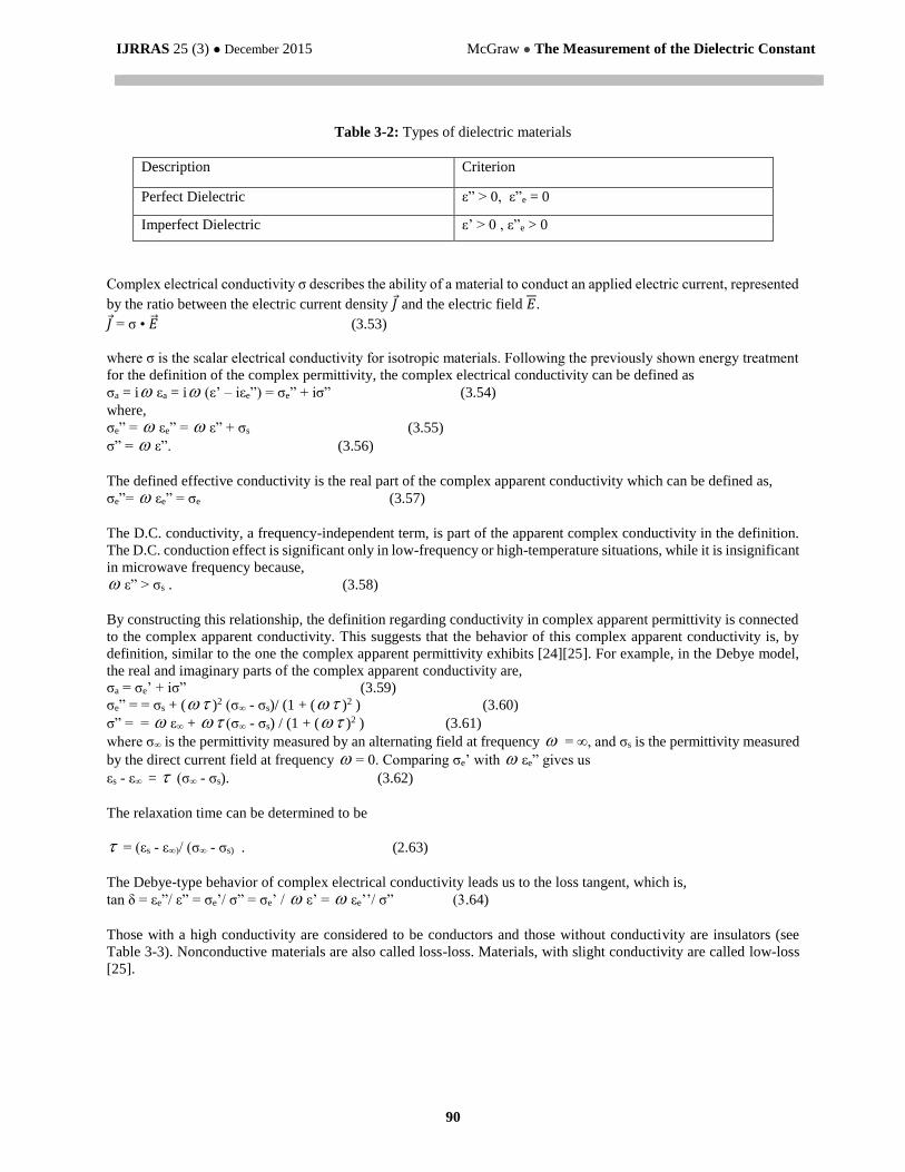
Figure 5. The Dielectric Constant of Wet Fine Concrete Block.
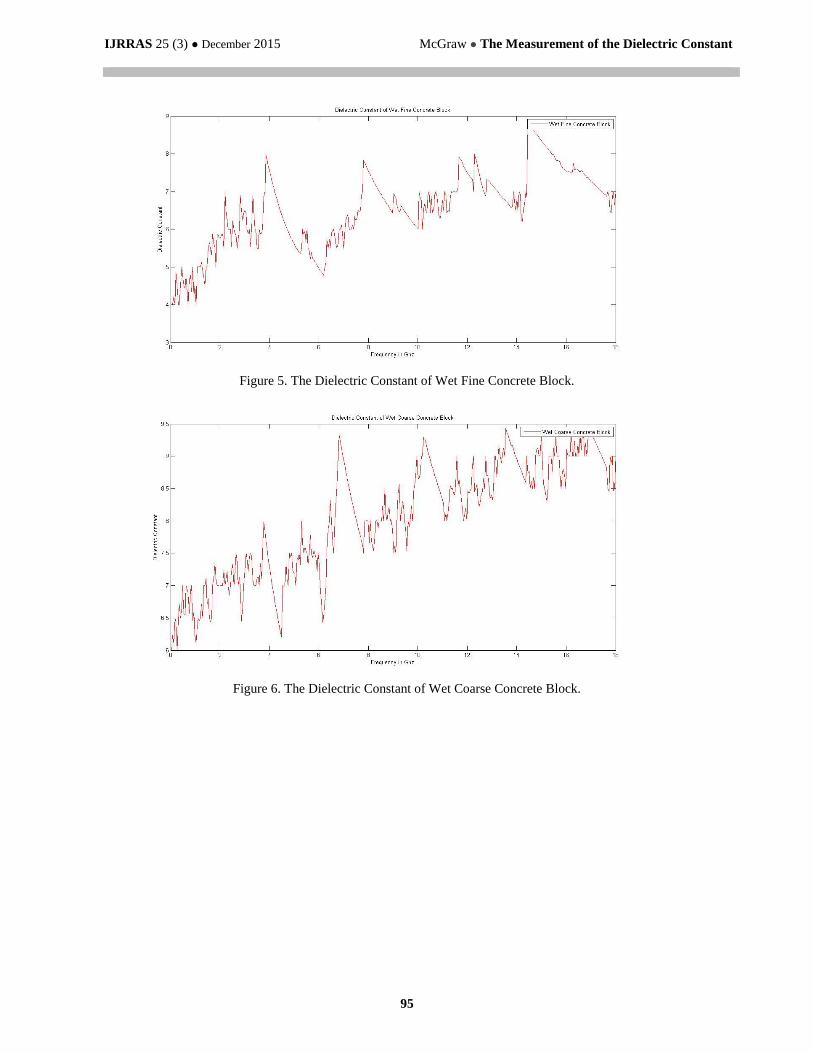
Figure 6. The Dielectric Constant of Wet Coarse Concrete Block.

IJRRAS 25 (3) ● December 2015 McGraw ● The Measurement of the Dielectric Constant
96
Figure 7. The Dielectric Constant of Wet Solid Concrete Block.
Figure 8. The Dielectric Constant of Saltwater Fine Concrete Block.
Figure 9. The Dielectric Constant of Saltwater Solid Concrete Block.
IJRRAS 25 (3) ● December 2015 McGraw ● The Measurement of the Dielectric Constant
97
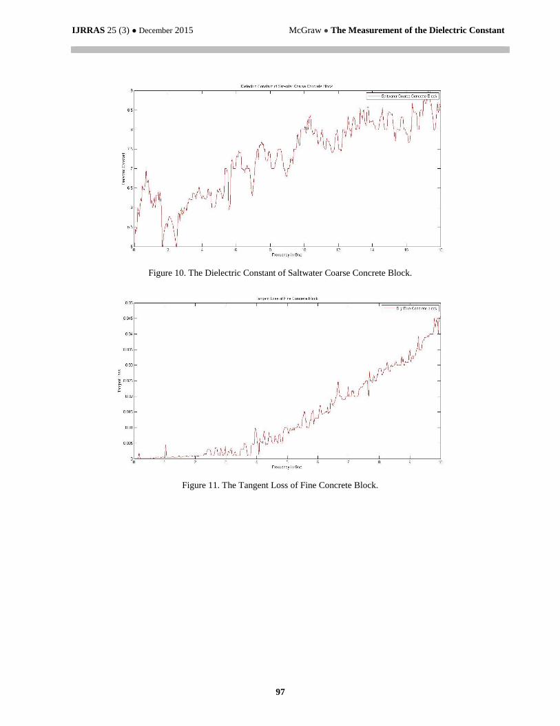
Figure 10. The Dielectric Constant of Saltwater Coarse Concrete Block.
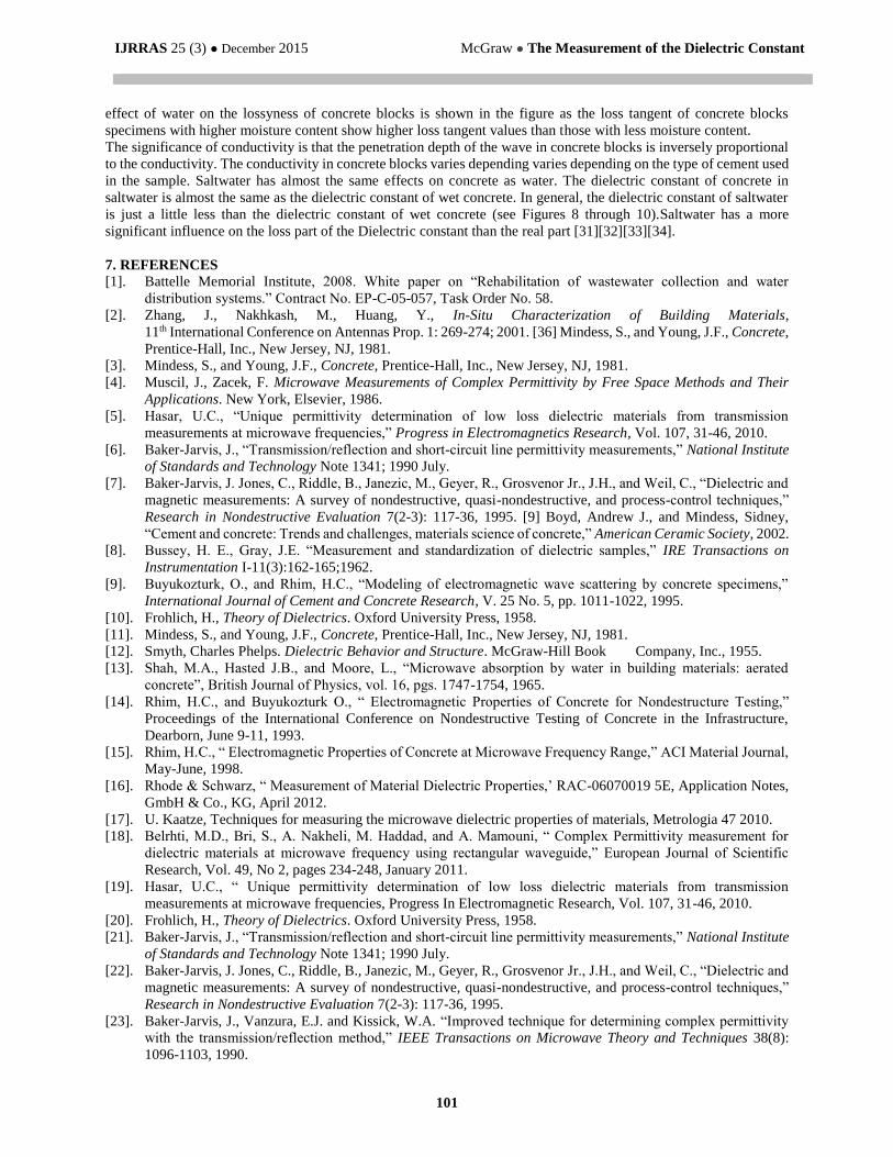
Figure 11. The Tangent Loss of Fine Concrete Block.

IJRRAS 25 (3) ● December 2015 McGraw ● The Measurement of the Dielectric Constant
98
Figure 12. The Tangent Loss of Coarse Concrete Block.
Figure 13. The Tangent Loss of a Solid Concrete Block.

IJRRAS 25 (3) ● December 2015 McGraw ● The Measurement of the Dielectric Constant
99
Figure 14: Conductivity of Concrete.

IJRRAS 25 (3) ● December 2015 McGraw ● The Measurement of the Dielectric Constant
100
Figure 15. Equipment and Computer Needed for Data Collecting.
6. SUMMARY
The dielectric constant of a material is not a constant, but is a function of the polarizability which is in turn a function
of frequency, temperature, local fields, applied field strength, availability and freedom of charge carriers within the
dielectric, and local field distortions. The dielectric conductivity is also affected by the same factors. This is because
the dielectric conductivity is a function not only of ohmic conductivity but also of the power consumed in polarizing
the material. Moisture and chloride are the two constituents which have the most effect on the dielectric properties of
concrete blocks. In general, the real part of the dielectric constant is larger when it is easier for the material to polarize,
meaning that the ions are mobile and there is little crystallization. The addition of chlorides increases the dielectric
constant, as does the amount of water. The dielectric constant decreases over curing time, because the amount of water
decreases during this time. Also, the dielectric constant of concrete is dependent on the constant of its aggregate: mixes
containing limestone have a higher constant than those containing granite, this correlates with the fact that limestone
itself has a higher constant than granite does [28][29][30].
There are certain concrete properties that influence the performance of concrete blocks. These properties include
concrete compressive strength, density, absorption, water cement ratio, cement content and type, and aggregates. All
of these factors would have an influence on the dielectric properties of concrete blocks. For example, the dielectric
constant for concrete with coarse aggregates is higher than concrete with fine aggregates. Concrete strength is a
function of many factors including, aggregates, cement material, manufacturing, curing process, and mix design.
These factors must also play a role in the dielectric constant of concrete blocks, since concrete blocks strength is a
function of these same factors[30][31].
7. CONCLUSION
In conclusion, it appears that at under dry conditions, the dielectric constant of concrete blocks does not vary much
over the measured frequency range (see Figures 2 through 4). However, the change of the dielectric constant of
concrete blocks becomes significant as the moisture level increases. Moisture content is one of the major constituents
which influence the electromagnetic properties of concrete blocks (see Figures 5 through 7). Loss factor of concrete
blocks is the imaginary part of the complex permittivity. The loss factor is divided by the dielectric constant over the
frequency range to obtain the loss tangent. The loss tangent of concrete blocks increases as frequency increases, the
IJRRAS 25 (3) ● December 2015 McGraw ● The Measurement of the Dielectric Constant
101
effect of water on the lossyness of concrete blocks is shown in the figure as the loss tangent of concrete blocks
specimens with higher moisture content show higher loss tangent values than those with less moisture content.
The significance of conductivity is that the penetration depth of the wave in concrete blocks is inversely proportional
to the conductivity. The conductivity in concrete blocks varies depending varies depending on the type of cement used
in the sample. Saltwater has almost the same effects on concrete as water. The dielectric constant of concrete in
saltwater is almost the same as the dielectric constant of wet concrete. In general, the dielectric constant of saltwater
is just a little less than the dielectric constant of wet concrete (see Figures 8 through 10).Saltwater has a more
significant influence on the loss part of the Dielectric constant than the real part [31][32][33][34].
7. REFERENCES
[1]. Battelle Memorial Institute, 2008. White paper on “Rehabilitation of wastewater collection and water
distribution systems.” Contract No. EP-C-05-057, Task Order No. 58.
[2]. Zhang, J., Nakhkash, M., Huang, Y., In-Situ Characterization of Building Materials,
11th International Conference on Antennas Prop. 1: 269-274; 2001. [36] Mindess, S., and Young, J.F., Concrete,
Prentice-Hall, Inc., New Jersey, NJ, 1981.
[3]. Mindess, S., and Young, J.F., Concrete, Prentice-Hall, Inc., New Jersey, NJ, 1981.
[4]. Muscil, J., Zacek, F. Microwave Measurements of Complex Permittivity by Free Space Methods and Their
Applications. New York, Elsevier, 1986.
[5]. Hasar, U.C., “Unique permittivity determination of low loss dielectric materials from transmission
measurements at microwave frequencies,” Progress in Electromagnetics Research, Vol. 107, 31-46, 2010.
[6]. Baker-Jarvis, J., “Transmission/reflection and short-circuit line permittivity measurements,” National Institute
of Standards and Technology Note 1341; 1990 July.
[7]. Baker-Jarvis, J. Jones, C., Riddle, B., Janezic, M., Geyer, R., Grosvenor Jr., J.H., and Weil, C., “Dielectric and
magnetic measurements: A survey of nondestructive, quasi-nondestructive, and process-control techniques,”
Research in Nondestructive Evaluation 7(2-3): 117-36, 1995. [9] Boyd, Andrew J., and Mindess, Sidney,
“Cement and concrete: Trends and challenges, materials science of concrete,” American Ceramic Society, 2002.
[8]. Bussey, H. E., Gray, J.E. “Measurement and standardization of dielectric samples,” IRE Transactions on
Instrumentation I-11(3):162-165;1962.
[9]. Buyukozturk, O., and Rhim, H.C., “Modeling of electromagnetic wave scattering by concrete specimens,”
International Journal of Cement and Concrete Research, V. 25 No. 5, pp. 1011-1022, 1995.
[10]. Frohlich, H., Theory of Dielectrics. Oxford University Press, 1958.
[11]. Mindess, S., and Young, J.F., Concrete, Prentice-Hall, Inc., New Jersey, NJ, 1981.
[12]. Smyth, Charles Phelps. Dielectric Behavior and Structure. McGraw-Hill Book Company, Inc., 1955.
[13]. Shah, M.A., Hasted J.B., and Moore, L., “Microwave absorption by water in building materials: aerated
concrete”, British Journal of Physics, vol. 16, pgs. 1747-1754, 1965.
[14]. Rhim, H.C., and Buyukozturk O., “ Electromagnetic Properties of Concrete for Nondestructure Testing,”
Proceedings of the International Conference on Nondestructive Testing of Concrete in the Infrastructure,
Dearborn, June 9-11, 1993.
[15]. Rhim, H.C., “ Electromagnetic Properties of Concrete at Microwave Frequency Range,” ACI Material Journal,
May-June, 1998.
[16]. Rhode & Schwarz, “ Measurement of Material Dielectric Properties,’ RAC-06070019 5E, Application Notes,
GmbH & Co., KG, April 2012.
[17]. U. Kaatze, Techniques for measuring the microwave dielectric properties of materials, Metrologia 47 2010.
[18]. Belrhti, M.D., Bri, S., A. Nakheli, M. Haddad, and A. Mamouni, “ Complex Permittivity measurement for
dielectric materials at microwave frequency using rectangular waveguide,” European Journal of Scientific
Research, Vol. 49, No 2, pages 234-248, January 2011.
[19]. Hasar, U.C., “ Unique permittivity determination of low loss dielectric materials from transmission
measurements at microwave frequencies, Progress In Electromagnetic Research, Vol. 107, 31-46, 2010.
[20]. Frohlich, H., Theory of Dielectrics. Oxford University Press, 1958.
[21]. Baker-Jarvis, J., “Transmission/reflection and short-circuit line permittivity measurements,” National Institute
of Standards and Technology Note 1341; 1990 July.
[22]. Baker-Jarvis, J. Jones, C., Riddle, B., Janezic, M., Geyer, R., Grosvenor Jr., J.H., and Weil, C., “Dielectric and
magnetic measurements: A survey of nondestructive, quasi-nondestructive, and process-control techniques,”
Research in Nondestructive Evaluation 7(2-3): 117-36, 1995.
[23]. Baker-Jarvis, J., Vanzura, E.J. and Kissick, W.A. “Improved technique for determining complex permittivity
with the transmission/reflection method,” IEEE Transactions on Microwave Theory and Techniques 38(8):
1096-1103, 1990.
IJRRAS 25 (3) ● December 2015 McGraw ● The Measurement of the Dielectric Constant
102
[24]. Constantine, A.B., Advanced Engineering Electromagnetics, John Wiley & Sons, 1989.
[25]. Cook, The Theory of the Electromagnetic Field, Prentice-Hall, 1975.
[26]. Weir, W.B., “Automatic measurement of complex dielectric constant and permeability at microwave
frequencies,” Proceedings of the IEEE 62(1): 33-36, 1974.
[27]. Su, W., Hazim, O.A., Al-Qadi, I. L., and Riad, M.C., “Permittivity of Portland Cement Concrete at Low RF
Frequencies,” Materials Evaluation, Apr. 1994, pp. 496-502.
[28]. Taherian, M.R., Yeun, D.J., Habashy, T.M., Kong, J.A., A coaxial-circular waveguide for dielectric
measurement, IEEE Tranaction Geoscience Remote Sensing, 29:321-330.,1991. [13] Clarke, R., A Guide to the
Dielectric Characterization of Materials at RF and Microwave Frequencies, National Physical Laboratory;
NPL; 2003.
[29]. Cole, R.H., “Correlation function theory of dielectric relaxation,” Journal of Chemical Physics 42: 637-
643,1964.
[30]. Debye, P., Polar Molecules, Dover Publications, Inc., 1929. Lea, F. M., The Chemistry of Cement and Concrete,
Chemical Publishing Company, Inc., New York, NY, 1971.
[31]. Mindess, S., and Young, J.F., Concrete, Prentice-Hall, Inc., New Jersey, NJ, 1981.
[32]. Lewin, L. Advanced Theory of Waveguides, London, England: Illiffe; 1951.
[33]. P. K. Mehta, Concrete: Structure, Properties and Materials, Prentice Hall, Englewood Cliffs, NJ, 1986.
[34]. Lynch, A.C., “Relationship between permittivity and loss tangent,” Proc. IEEE 118: 244-246; 1971.


![c Consult author(s) regarding copyright matters · dielectric material with dielectric constant around ~3.1 at 1 KHz [22]. Due to its low dielectric constant (low-K), PC dielectric](https://cdn.vdocument.in/doc/165x107/5e8ef91e49d7e74eaa111a6e/c-consult-authors-regarding-copyright-matters-dielectric-material-with-dielectric.jpg)


