Download - The microeconomics of the price mechanism


UNIVERSITY OFILLINOIS LIBRARY
AT URBANA-CHAMPAIGNBOOKSTACKS

Digitized by the Internet Archive
in 2011 with funding from
University of Illinois Urbana-Champaign
http://www.archive.org/details/microeconomicsof91163brem


Faculty Working Paper 91-0163
330B3851991:163 COPY
The Microeconomics of the Price Mechanism
Tbe Ubrarv ottt^
Hans BremsDepartment of Economics
Lectures to Be Given at the Charles University oj"PragueWinter 1991/1992
Bureau of Economic and Uu.sincsi Research
College of Commerce and Business Adminisiraiion
University of Illinois at l,'rbana-C;hampaign


BEBRFACULTY WORKING PAPER NO. 9 1 -0 1 63
College of Commerce and Business Administration
University of Illinois at (Jrbana-Champaign
September 1991
The Microeconomics of the Price Mechanism
Hans BremsDepartment of Economics
University of Illinois
1206 South Sixth Street
Champaign, !L 61820

HariB Brema
Lectures on the Price Mechanism^ Charles University of Prague
Winter 1991/1992

MICROECONOMICS

PREFACE
Microeconomics comes in two parts, price theory and allo-
cation theory. The present minicourse will develop both parts
as well as their late-nineteenth-century integration. The
course closes with an elementary restatement of von Neumann's
proof of the existence of a general economic equilibrium.
Modern economic theory comes in mathematical form, and
no other form will do. The course confines itself to elemen-
tary algebra and calculus. A reader needing help will find some
in our appendix.
Chapter 1 will be published in the winter 1991 issue of
History of Political Economy. Chapters 2 and 3 are newly written
but based on material published in chapters 6 and 11, respectively
of my Pioneering Economic Theory 1630-1980, A Mathematical Resta-
tement , Baltimore: Johns Hopkins University Press, 1986.
University of Illinois, September 1991
It is not from the henevolenoe of the hutohev^
the brewerJ or the baker^ that we expect oia? di-n-
ner, but from the-lr regard to the-lr own interest
Adam Smithj Wealth of Nations
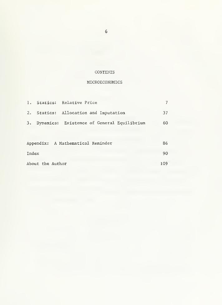
CONTENTS
MICROECONOMICS
1. Statics: Relative Price 7
2. Statics: Allocation and Imputation 37
3. Dynamics: Existence of General Equilibrium 60
Appendix: A Mathematical Reminder 86
Index 90
About the Author 109

Copyright Duke University Press
CHAPTER 1
STATICS: RELATIVE PRICE
Abstraat
Qmtitlcn trisd to build a land theory of value and auaeeeded^
His relative-price solution was self-oontained: it had no factor
prices in it but only inpict-cutput coeffieisTvts* Marx tried to
build a labor theory of value but failed: his relative-pTnce ex-
pression still had the rate of interest in it» Smith and the
nsoelassicals used the full trinity of capital^ labor, and land and
node no atteapt to reduce it to any single factor* All factor
prices appeared in the relative-price expressions—pointing towards
a general-equilibriim model,
I. INTRODUCTION
1. Microeconomics
Microeconomic theory considers an economy producing more than
one good and comes in tv/o parts, price theory and allocation theory.
Price theory determines the relative price of such goods. Allocation
theory determines the physical quantities transacted of each good,
i.e., how inputs are allocated among outputs and outputs among house-
holds. In the late nineteenth century price and allocation theory
fell into place and came to be seen as inseparable parts of general
equilibrium. We begin with price theory.
2. Variables, Parameters, and Solutions
: We try to explain economic variables by building models of them.
A model is a system of equations containing variables related to one
another via parameters. A parameter is a quantity fixed by the investi-
gator using information comdng from outside the model. For example,
a microeconomic model may use technology, preferences, resources, and
legal institutions as its parameters.
Having built our models, we try to solve them. By a solution for a
variable we mean an equation having that variable on its left-hand side
and nothing but parameters on its right-hand side. Since the distinction
between variables and parameters is so important—and may differ among
models—we shall open each chapter with a complete list of its variab-
les and its parameters.
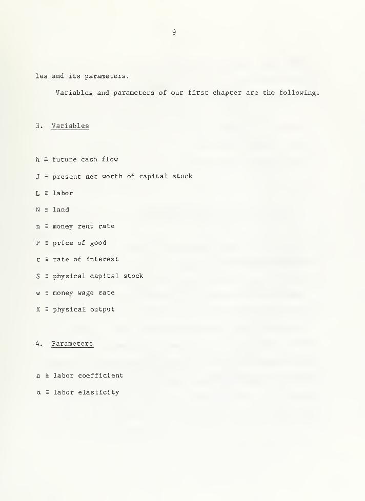
Variables and parameters of our first chapter are the following,
3. Variables
h = future cash flow
J E present net worth of capital stock
L s labor
N = land
n = money rent rate
P 5 price of good
r = rate of interest
S s physical capital stock
w = money wage rate
X = physical output
4. Parameters
a = labor coefficient
a = labor elasticity

10
b s land coefficient
3 = land elasticity
c = capital coefficient
Y = capital elasticity
j = joint factor productivity
m = labor's manner of living
u = useful life of capital stock
II. CANTILLON
1 . Production Technology
Cantillon certainly knew no diminishing returns— indeed nobody
knew thera before Turgot [1767 (1844: 418-A33), (1977: 109-122)].
Did Cantillon know that production takes time? In other parts of
his work he was well aware of it, but in the passages [1755 (1931:
Al)] developing his famous "Par between Land and Labour" he ignored
capital. Let us restate his par mathematically.
11
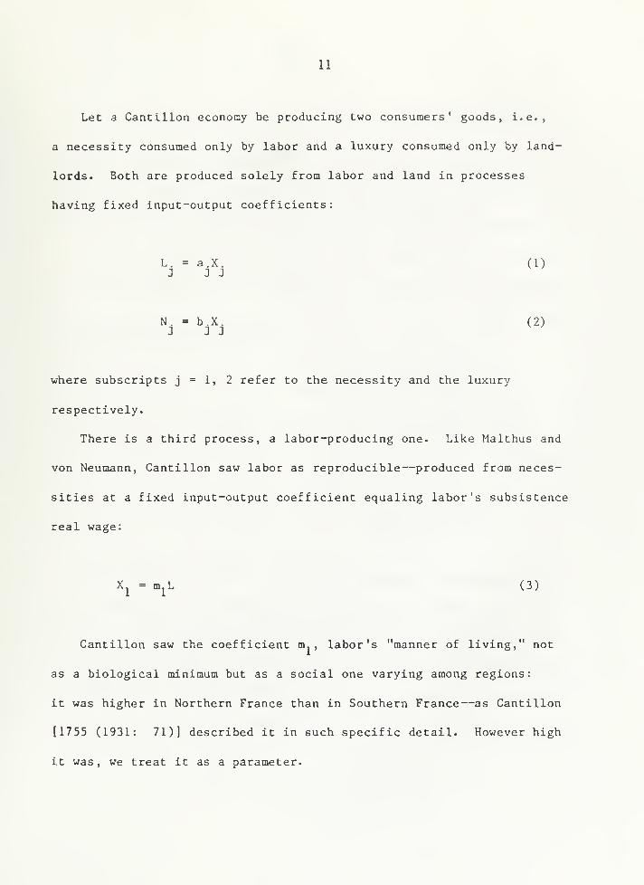
Let a Cantillon economy be producing two consumers' goods, i.e.,
a necessity consumed only by labor and a luxury consumed only by land-
lords. Both are produced solely from labor and land in processes
having fixed input-output coefficients:
L. = a.X. (1)3 J J
N. = b.X. (2)J J J
where subscripts j = 1, 2 refer to the necessity and the luxury
respectively.
There is a third process, a labor-producing one. Like Malthus and
von Neumann, Cantillon saw labor as reproducible—produced from neces-
sities at a fixed input-output coefficient equaling labor's subsistence
real wage:
X^ = m^L (3)
Cantillon saw the coefficient m. , labor's "manner of living," not
as a biological minimum but as a social one varying among regions:
it was higher in Northern France than in Southern France—as Cantillon
[1755 (1931: 71)] described it in such specific detail. However high
it was, we treat it as a parameter.
12
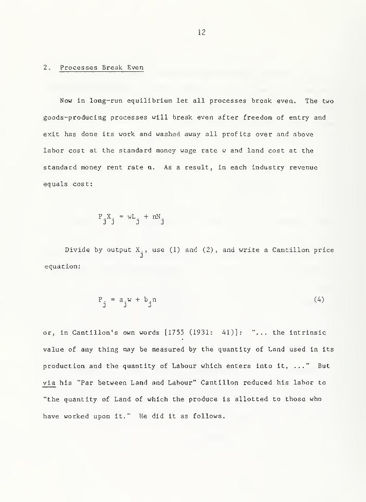
2 , Processes Break Even
Now in long-run equilibrium let all processes break even. The two
goods-producing processes will break even after freedom of entry and
exit has done its work and washed away all profits over and above
labor cost at the standard money wage rate w and land cost at the
standard money rent rate n. As a result, in each industry revenue
equals cost:
P.X. = wL. + nN.2 2 2 2
Divide by output X., use (1) and (2), and write a Cantillon price
equation:
P. = a.w + b.n (4)2 2 2
or, in Cantillon's own words [1755 (1931: 41)]: "... the intrinsic
value of any thing may be measured by the quantity of Land used in its
production and the quantity of Labour which enters into it, ..." But
via his "Par between Land and Labour" Cantillon reduced his labor to
"the quantity of Land of which the produce is allotted to those who
have worked upon it." He did it as follows.

13
The labor-producing process will break, even, because [1755 (1931:
83)] "Men multiply like Mice in a bam if they have unlimited Means of
Subsistence." Here, too, rrvenue equals cost or, in more familiar
terms, the wage bill equals the value of labor's consumption:
wL = P^Xj
3. Solution for Relative Price
Insert (3), divide L away, and write a Cantillon wage equation;
w = m^P^ (5)
Insert (5) into (4) and write the Cantillon price equation;
P .= a.m.P, + b .n
J J 1 1 3
which is a system of two equations in three unknowns n, P, , and P«.
Solve it for P. and P2 , divide former by latter, let n cancel, and
write Cantillon' s relative price
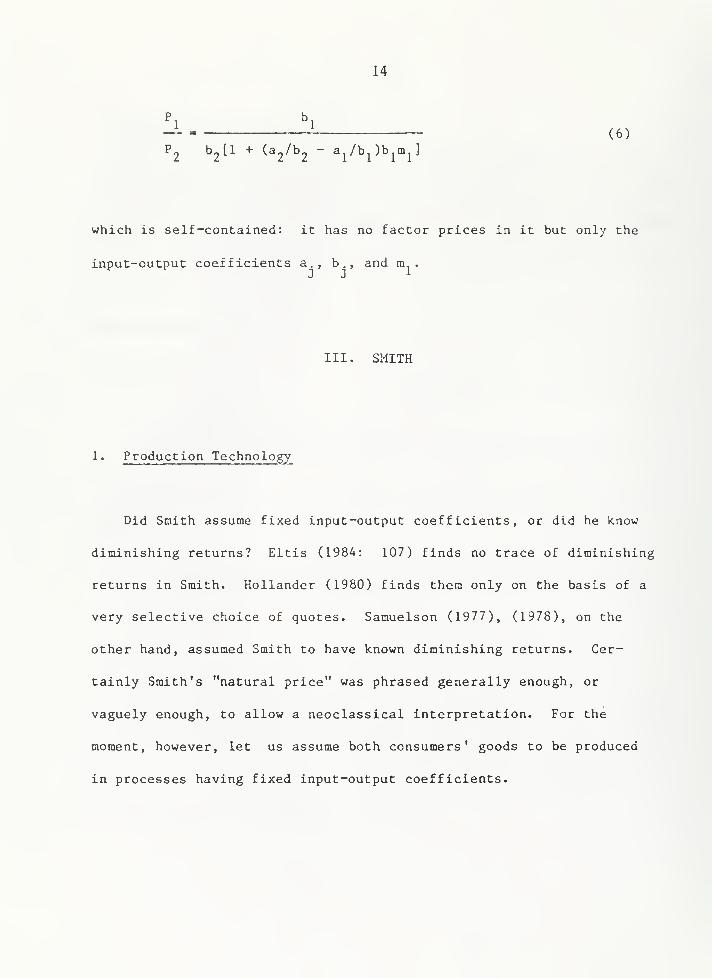
14
— (6)P2 b2[l + (a2/b2 - a^/b^)b^m^]
which is self-contained: it has no factor prices in it but only the
input-output coefficients a., b., and m,
.
J J 1
III. SMITH
1. Production Technology
Did Smith assume fixed input-output coefficients, or did he know
diminishing returns? Eltis (1984: 107) finds no trace of diminishing
returns in Smith. Hollander (1980) finds thera only on the basis of a
very selective choice of quotes. Samuelson (1977), (1978), on the
other hand, assumed Smith to have known diminishing returns. Cer-
tainly Smith's "natural price" was phrased generally enough, or
vaguely enough, to allow a neoclassical interpretation. For the
moment, however, let us assume both consumers' goods to be produced
in processes having fixed input-output coefficients.
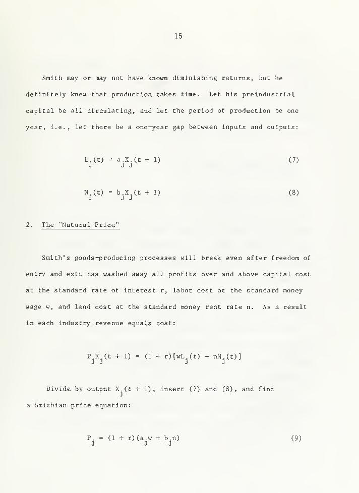
15
Smith may or may not have known diminishing returns, but he
definitely knew that production takes time. Let his preindustrial
capital be all circulating, and let the period of production be one
year, i.e., let there be a one-year gap between inputs and outputs:
L^(t) = a^X^Ct + 1) (7)
N.(t) = b.X.(t + 1) (8)J J J
2. The "Natural Price"
Smith's goods-producing processes will break even after freedom of
entry and exit has washed away all profits over and above capital cost
at the standard rate of interest r, labor cost at the standard money
wage w, and land cost at the standard money rent rate n. As a result
in each industry revenue equals cost:
P.X.(t +!)=(!+ r)[wL.(t) + nN.(t)]3 2 J J
Divide by output X.(t + 1), insert (7) and (8), and find
a Smithian price equation:
P. = (1 + r)(a.w + b.n) (9)J J J

16
Here is Smith's [1776 (1805: book I, chapter 7)] "natural price,"
i.e., a price "neither more nor less than what is sufficient to pay
the rent of the land, the wages of the labour, and the profits of the
stock employed in raising, preparing, and bringing it to market,
according to their natural rates."
3. Was Labor Reproducible?
Did Smith, like Cantillon, have a third process producing labor
from necessities at a fixed input-output coefficient equaling labor's
subsistence real wage? To be sure, Smith [1776 (1805: book I,
chapter 8)] did observe that "every species of animals naturally
multiplies in proportion to the means of their subsistence..." And,
for humans, Smith saw such subsistence not as a biological raininum but
as a social one varying among nations. Indeed it was higher in North
America than in England.
Yet, if ever tempted to build such a labor-producing process into
his price theory. Smith withstood the temptation. Nothing like
Cantillon 's par between land and labor occurred to Smith. Nowhere
did he reduce labor to land.
We, too, shall withstand the temptation, leave Smith's "natural
price" the way he left it, and find his relative price.
17
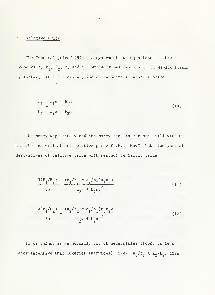
4. Relative Price
The "natural price" (9) is a system of two equations in five
unknowns n, P , P , r, and w. Write it out for j = 1, 2, divide former
by latter, let 1 + r cancel, and write Saith's relative price
P a.w + b n— = — — (10)
^2 ^2" "" ^2"
The money wage rate w and the money rent rate n are still with us
in (10) and will affect relative price P./P^. How? Take the partial
derivatives of relative price with respect to factor price
3w (aw + b n)
3(P,/P,) (a^/b - a /b )b b wL_A_ = _^_J i ^^ (12)3n (aw + b n)
If we think, as we normally do, of necessities (food) as less
labor-intensive than luxuries (services), i.e., Si/b. < a^/b„, then
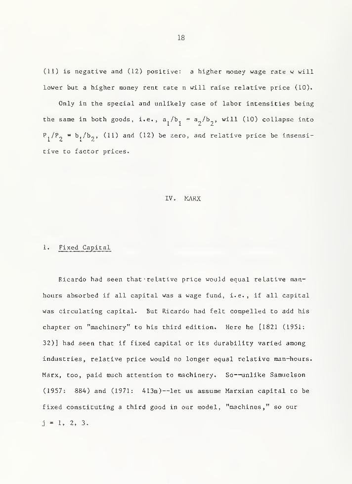
18
(11) is negative and (12) positive: a higher money wage rate w will
lower but a higher money rent rate n will raise relative price (10).
Only in the special and unlikely case of labor intensities being
the same in both goods, i.e., a,/b = a /b , will (10) collapse into
P./P„ = b./b^, (11) and (12) be zero, and relative price be insensi-
tive to factor prices.
IV. KARX
1. Fixed Capital
Ricardo had seen that relative price would equal relative man-
hours absorbed if all capital was a wage fund, i.e., if all capital
was circulating capital. But Ricardo had felt compelled to add his
chapter on "machinery" to his third edition. Here he [1821 (1951:
32)] had seen that if fixed capital or its durability varied among
industries, relative price would no longer equal relative man-hours.
Marx, too, paid much attention to machinery. So—unlike Samuelson
(1957: 884) and (1971: A13n)—let us assume Marxian capital to be
fixed constituting a third good in our model, "machines," so our
j = 1, 2, 3.
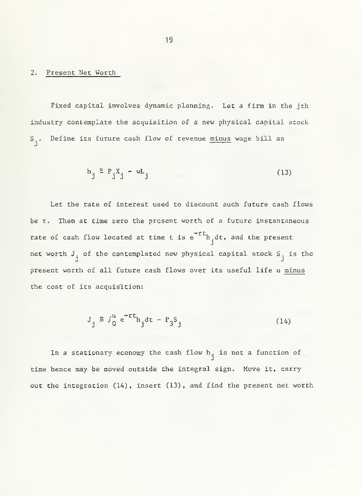
19
2. Present Net Worth
Fixed capital involves dynamic planning. Let a firm in the jth
industry contemplate the acquisition of a new physical capital stock
S . . Define its future cash flow of revenue minus wage bill asJ
h. = P.X. - wL. (13)
Let the rate of interest used to discount such future cash flows
be r. Then at time zero the present worth of a future instantaneous
rate of cash flow located at time t is e n.dt, and the presentJ
net worth J, of the contemplated new physical capital stock S. is the
present worth of all future cash flows over its useful life u minus
the cost of its acquisition:
J. E /^ e-^Vdt - P3S. (14)
In a stationary economy the cash flow h. is not a function of
time hence may be moved outside the integral sign. Move it, carry
out the integration (14), insert (13), and find the present net worth

20
, -ru1 - e
J. = (P.X. - wL.) - P_S. (15)J ^ J J 3 3 J
3. Production Technology
Ricardo had known diminishing returns but may not have realized
that they would make his labor and capital coefficients vary with his
margins of cultivation. Marx ignored land and with it diminishing
returns. We welcome such simplification allowing us to treat labor
and capital coefficients as technological parameters:
L. = a.X. (16)J 3 J
S. = c.X. (17)J J J
Ricardo 's durable producers' goods had been made from labor alone,
To his credit, to Mar^ it also took producers' goods to produce pro-
ducers' goods: a. > and c. > for i = 1, 2, 3.J J
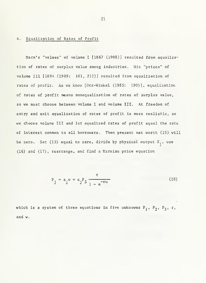
21
A. Equalization of Rates of Profit
Marx's "values" of volume I (1867 (1908)] resulted from equaliza-
tion of rates of surplus value among industries. His "prices" of
volume III [1894 (1909: 181, 212)] resulted from equalization of
rates of profit. As we know [Ott-Winkel (1985: 190)], equalization
of rates of profit means nonequalization of rates of surplus value,
so we must choose between volume I and volume III. At freedom of
entry and exit equalization of rates of profit is more realistic, so
we choose volume III and let equalized rates of profit equal the rate
of interest common to all borrowers. Then present net worth (15) will
be zero. Set (15) equal to zero, divide by physical output X., use
(16) and (17), rearrange, and find a Marxian price equation
P. = a.w + c.P_ (18)
which is a system of three equations in five unknowns P, , P^f ^3 » ^>
and w.
22
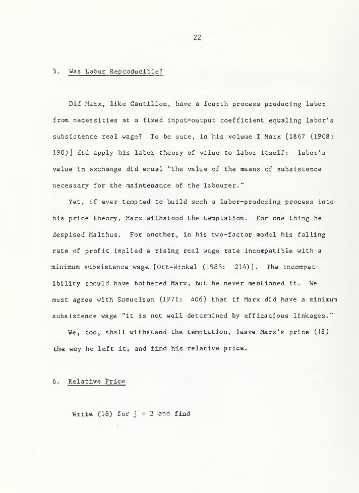
5. Was Labor Reproducible?
Did Marx, like Cantillon, have a fourth process producing labor
from necessities at a fixed input-output coefficient equaling labor's
subsistence real wage? To be sure, in his volume I Marx (1867 (1908:
190) J did apply his labor theory of value to labor itself: labor's
value in exchange did equal "the value of the means of subsistence
necessary for the maintenance of the labourer."
Yet, if ever tempted to build such a labor-producing process into
his price theory, Marx withstood the temptation. For one thing he
despised Malthus. For another, in his two-factor model his falling
rate of profit implied a rising real wage rate incompatible with a
minimum subsistence wage [Ott-Winkel (1985: 214)]. The incompat-
ibility should have bothered Marx, but he never mentioned it. We
must agree with Samuelson (1971: A06) that if Marx did have a minimum
subsistence wage "it is not well determined by efficacious linkages."
We, too, shall withstand the temptation, leave Marx's price (18)
the way he left it, and find his relative price.
6. Relative Price
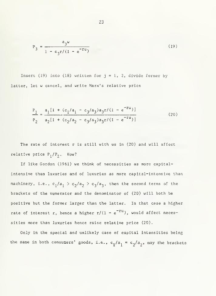
Write (18) for j = 3 and find
23
awP. = (19)
1 - C3r/(1 - e '")
Insert (19) into (18) written for j = 1, 2, divide former by
latter, let w cancel, and write Marx's relative price
P^ aj[l +^^i/^i
~ C3/a2)a2r/(l - e )]
(20)
The rate of interest r is still with us in (20) and will affect
relative price Pi/Po- ^°"'^
If like Gordon (1961) we think, of necessities as more capital-
intensive than luxuries and of luxuries as more capital-intensive than
machinery, i.e., c,/a, > c-^/a- > c-,/a-,, then the second terms of the
brackets of the numerator and the denominator of (20) will both be
positive but the former larger than the latter. In that case a higher
rate of interest r, hence a higher r/(l - e ), would affect neces-
sities more than luxuries hence raise relative price (20).
Only in the special and unlikely case of capital intensities being
the same in both consumers' goods, i.e., c./a. = c„/a , may the brackets
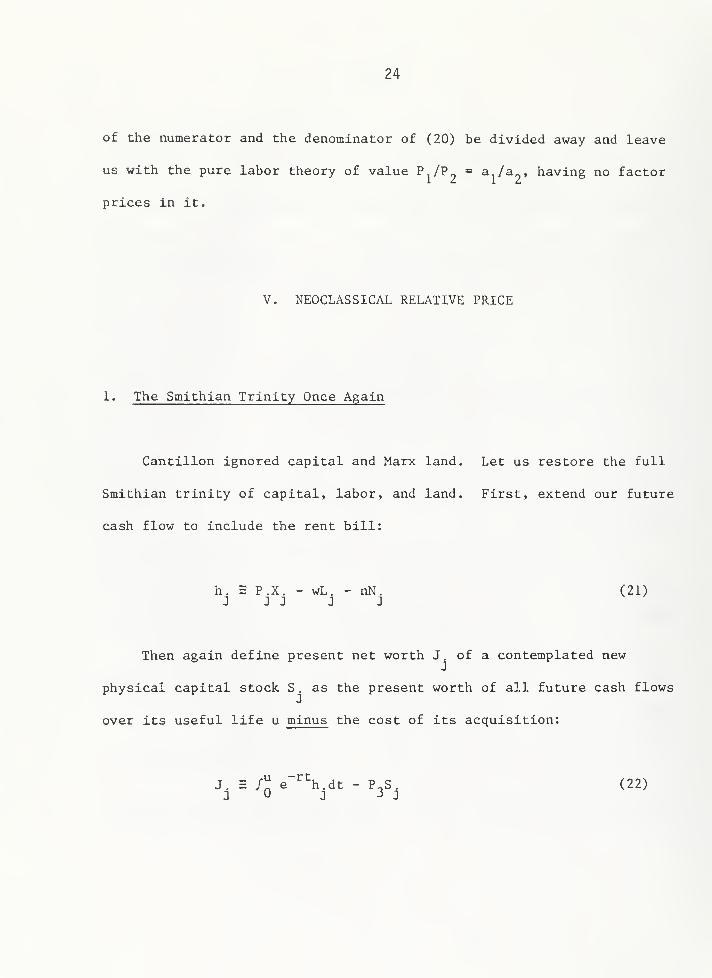
24
of the numerator and the denominator of (20) be divided away and leave
us with the pure labor theory of value P,/P^ = ^1/^9 » having no factor
prices in it.
V. NEOCLASSICAL RELATIVE PRICE
1. The Smithian Trinity Once Again
Cantillon ignored capital and Marx land. Let us restore the full
Smithian trinity of capital, labor, and land. First, extend our future
cash flow to include the rent bill:
h. = P.X. - wL. - nN. (21)J J J J J
Then again define present net worth J. of a contemplated new
physical capital stock S . as the present worth of all future cash flows
over its useful life u minus the cost of its acquisition:
J. = /;j e ""^h.dt - P„S. (22)J J 3 J
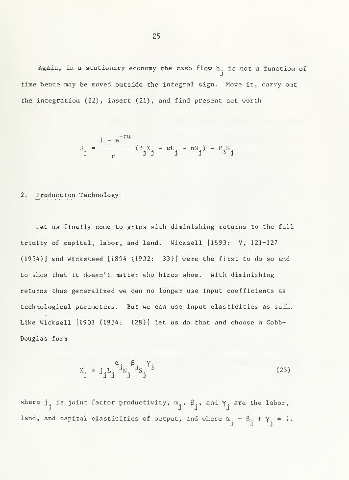
25
Again, in a stationary economy the cash flow h. is not a function of
time hence may be moved outside the integral sign. Move it, carry out
the integration (22), insert (21), and find present net worth
1~^^
1 - e
J. = (P.X. - wL. - nN.) - P»S.
2. Production Technology
Let us finally come to grips with diminishing returns to the full
trinity of capital, labor, and land. Wicksell [1893: V, 121-127
(1954)] and Wicksteed [1894 (1932: 33)] were the first to do so and
to show that It doesn't matter who hires whom. With diminishing
returns thus generalized we can no longer use input coefficients as
technological parameters. But we can use input elasticities as such.
Like Wicksell [1901 (1934: 128)] let us do that and choose a Cobb-
Douglas form
a. 3. y.X. = j.L. ^N. ^S. ^ (23)J J J J J
where j. is joint factor productivity, a., 3.> and y. are the labor,
land, and capital elasticities of output, and where a. +3. + Y. = 1
J J J
26
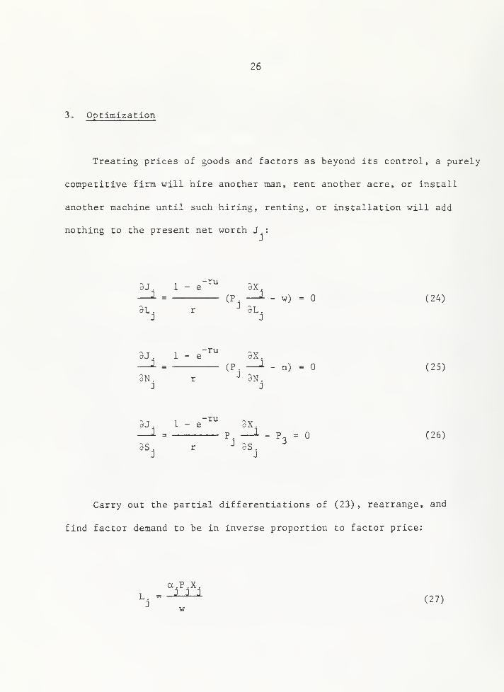
3. Optimization
Treating prices of goods and factors as beyond its control, a purely
competitive firm will hire another man, rent another acre, or install
another machine until such hiring, renting, or installation will add
nothing to the present net worth J .
:
dJ. 1-ru
- e 9X2
(^nJ - w) =
3L.J
rJ
9L.
9J. 1-ru
- e 9X.J
(^J - n) =
3N. rJ 3N.
2
(24)
(25)
3J. 1 - e"^"" 3X.^ = P. —^ - P^ = (26)
as. r ^ 3S. ^
J 3
Carry out the partial differentiations of (23) , rearrange, and
find factor demand to be in inverse proportion to factor price:
a,P,X,
(27)L. =-^-J-i
w

27
3.P.X.
N. = ^ ^ ^ (28)J
Y.P.X.S. = ^—LJ (29)J P3r/(1 - e-^^)
Multiply across, add (27), (28), and (29), and notice in pass-
ing Wicksteed's [1894 (1932: 37)] product-exhaustion theorem
wL. + nN. + P_S.r/(l - e~^^) = P.X..
4. Relative Price
Raise (27) to the power a., (28) to the power 3-» and (29) to the
power y.. Multiply the three equations. Use (23) and find an X. on
both the left-hand and the right-hand side of their product. Divide
it away, rearrange the rest, and find the neoclassical price equation
1 w °^j n ^j 1"^j P r ^j
P, = — (—) (—) (—) (^--—
)
(30)
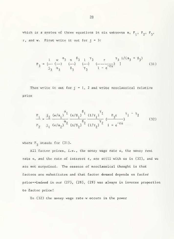
28
which is a systera of three equations in six unknowns n, P , P„, P,
r, and w. First write it out for j = 3;
1 w "3 n ^3 1 ^3 r ^3 ^/^°'3 ^ ^3^
P. = [— (—
)
(—
)
(—
)
( ) ] (31)3 . n ,
~rUJ3 a3 B3 Y3 1 - e
Then write it out for j = 1, 2 and write neoclassical relative
price
^1 °l ^1P j (w/a ) (n/6,) (1/y,) P.r ^1 '^2
- =-—4 4 -r^
—^
^''^
^2 Ji ^"/'^2^ ^ ^"/^2^ ^ ^^^^2^ ^ 1 - e''''
where P stands for (31).
All factor prices, i.e., the money wage rate w, the money rent
rate n, and the rate of interest r, are still with us in (32), and we
are not surprised. The essence of neoclassical thought is that
factors are substitutes and that factor demand depends on factor
price—indeed in our (27), (28), (29) was always in inverse proportion
to factor price!
In (32) the money wage rate w occurs in the power
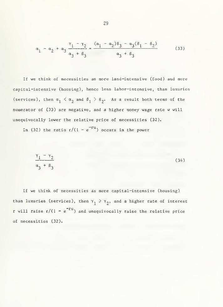
29
a - a_ + a- = (33)
«3 ^ ^3 <^3 -^ ^3
If we think of necessities as more land-intensive (food) and more
capital-intensive (housing), hence less labor-intensive, than luxuries
(services), then a < a„ and 6, > 6^. As a result both terras of the
numerator of (33) are negative, and a higher noney wage rate w will
unequivocally lower the relative price of necessities (32).
In (32) the ratio r/(l - e ) occurs in the power
— (3A)
^3 ^ ^3
If we think, of necessities as more capital-intensive (housing)
than luxuries (services), then y > y„, and a higher rate of interest
r will raise r/(l - e ) and unequivocally raise the relative price
of necessities (32).

30
VI. SUMMARY AND CONCLUSION
By ignoring capital and by reducing labor to land, Cantillon tried
to build a land theory of value. He succeeded. His relative-price
solution (6) was self-contained: it had no factor prices in it but
only input-output coefficients. It was indeed a solution.
By ignoring land and by reducing machines to labor, Marx tried to
build a labor theory of value. He failed: his relative-price
expression (20) still had the rate of interest in it.
Smith and neoclassicals used the full trinity of capital, labor,
and land and made no attempt to reduce it to any single factor. Not
surprisingly, all their factor prices still appeared in their
relative-price expressions (10) and (32).
To Smith natural price was a one-way causal relationship between
goods price and factor prices: it was because 2 francs were paid out
in rent, 2 francs in wages, and 1 franc in interest that this bottle
of wine sells for 5 francs, as Walras [187A-1877 (1954: 211)] put it.
We know better. To us a solution for a variable is an equation
having that variable on its left-hand side and nothing but parameters
31
on its right-hand side. But on the right-hand sides of our (10)
,
(20), and (32) we find the rates n, r, or w of rent, interest or
wages, and they are not parameters but variables remaining to be
explained in a general-equilibrium model.
We have work to do, then. Some of it was first done in Prague.
as we shall see in our next chapter.
32
FOOTNOTE
*For careful reading and helpful suggestions, the author is
indebted to his friend and colleague Dr. J. van Daal of the Erasmus
University of Rotterdam. To an anonymous referee of History of Political
Economy he is equally indebted.
Earlier drafts of the present chapter were read at the Western Economic
Association International meeting in San Diego in July 1990, at the Scandi-
navian meeting on the history of economic thought in Gothenburg in Septem-
ber 1990, and at the Erich-Schneider Seminar in Kiel in November, 1990.
For critical comments the author is indebted to Jurg Niehans (California)
,
Claes-Henric Siven (Stockholm) , and Horst Herberg (Kiel)
.

33
REFERENCES
R. Cantillon, Essai sur la nature du commerce en general , written
around 1730, published 1755 referring to a fictitious publisher:
"A Londres, Chez F. Gyles, dans Holborn"; reprinted, Boston, 1892;
edited and translated into English by Henry Higgs, C.B., London,
1931; translated into German with an introduction by F. A. Hayek,
Jena, 1931; republished in French, Paris, 1952.
W. Eltis, The Classical Theory of Economic Growth , London, 1984.
R. A. Gordon, "Differential Changes in the Prices of Consumers' and
Capital Goods," Amer. Econ. Rev. , Dec. 1961, 5_1_, 937-957.
S. Hollander, "On Professor Samuelson's Canonical Classical Model of
Political Economy," J. Econ. Lit., June 1980, 18, 559-574.

34
K. Marx, Das Kapltal: Krltlk der polltlschen Oekonomte , vol. I,
Per Produktlonsprocess des Kapltals , Hamburg, 1867; translated as
Capital: A Critique of Political Economy , vol. I, The Process of
Capitalist Production by Samuel Moore and Edward Aveling, edited
by Friedrich Engels, revised and amplified according to the fourth
German edition by Ernest Untermann, Chicago, 1908.
, Das Kapltal: Kritik der polltlschen Oekonomie, vol. Ill,
Der Gesamtprocess der kapitalistischen Produktion , Hamburg, 189A;
translated as Capital: A Critique of Political Economy , vol. Ill,
The Process of Capitalist Production as a Whole by Ernest
Untermann, edited by Friedrich Engels, Chicago, 1909.
Ott, A. E. , and Winkel, H., Geschichte der theoretischen
Volkswirtschaf tslehre , Gottingen, 1985.
D. Ricardo, The Principles of Political Economy and Taxation , third
edition, London, 1821, reprinted in The Works and Correspondence
of David Ricardo , P. Sraffa and M. H. Dobb (eds.), vol. I,
New York, 1951.
P. A. Samuelson, "Wages and Interest: A Modem Dissection of Marxian
Economic Models," Amer. Econ. Rev., Dec. 1957, A7, 884-912.
35
, "Understanding the Marxian Notion of Exploitation: A
Summary of the So-Called Transformation Problem Between Marxian
Values and Competitive Prices," J» Econ. Lit. , June 1971, 9_,
399-431.
, "Insight and Detour in the Theory of Exploitation: A
Reply to Baumol," J. Econ. Lit. , Mar. 1974, J^, 62-70.
, "A Modern Theorist's Vindication of Adam Smith," Amer.
Econ. Rev. , Feb. 1977, 67, 42-49.
, "The Canonical Classical Model of Political Economy,
J. Econ. Lit. , Dec. 1978, J_6,1415-1434.
A. Smith, An Inquiry into the Nature and Causes of the Wealth of
Nations , London, 1776, new edition, Glasgow, 1805.
A. R. J. Turgot, "Observations sur le Memoire de M. de Saint-Peravy ,
"
Limoges, 1767, in E. Daire (ed.), Oeuvres de Turgot , Paris, 1844,
and translated as "Observations on a Paper by Saint-Peravy on the
Subject of Indirect Taxation," in P. D. Groenewegen, The Economics
of A» R. J. Turgot, The Hague, 197 7.
L. Walras, Elements d'economie politique pure , Lausanne, Paris, and
Basle, 1874-1877, translated as Elements of Pure Economics or the
Theory of Social Wealth by W. Jaffe, Horaewood 111., 1954.
K. Wicksell, Ueber Wert, Kapital und Rente , Jena, 1893, translated as
Value, Capital and Rent by S. H. Frohwein, London, 1954.
, Forelasningar i nationalekonomi, I, Lund, 1901, translated
as Lectures on Political Economy , I by E. Classen and edited by
Lionel Robbins , London, 1934.
P. H. Wicksteed, The Co-ordination of the Laws of Distribution,
London, 1894, reprinted by the London School of Economics in 1932
with 14 misprints corrected but not the dP /dC on mid-page 32,
which should have been dP/dL.
37
Copyright Johns Hopkins University Press
CHAPTER 2
STATICS: ALLOCATION AND IMPUTATION
Abstrcuat
fhs previous chapter pointed tooards a gengrat-equilibrim
model* The pi>esent chapter begins with Vieser's allocation and
imputation. Outputs will be substitutes in a utility function.
Inputs will be substitutes in a production function* Households
will nuadmiMe utility and industry will maximize profits, A
price mechanism will allocate inputs among outputs and outputs
aaong households. The chapter will build and solve a Vieser
modal of a stationary economy with two outputs, two inputs, and
two households.
38
I. INTRODUCTION
1. Allocation
We turn to the second part of microeconomics: how are goods allo-
cated among uses? Allocation must reflect preferences, but not until
the end of the nineteenth century did preferences enter mainstream
microeconomics
.
To Menger [1871 (1950)] goods were valued because needed, and
their value would depend on the need satisfied by the last unit of
goods available. That need would be the least important need: take
the last unit away, and the consumer could still satisfy his
higher-priority needs and merely go without the satisfaction of
his least important one. That was all, but with that Menger had put
economic theory on a new foundation.
2. Imputation
But Menger confined himself to households and their demand for

39
outputs. For industry and its demand for inputs we must turn to
Friedrich von Wieser (1851-1926) who taught at the Charles University
of Prague 1884-1903 where he wrote his Per natilrliche Werth
Goods were valued because needed: outputs satisfied needs di-
rectly, inputs satisfied them indirectly. How needed inputs were
would depend on two things, first, how productive inputs were in
producing outputs and, second, how needed such outputs were. Inputs
would be valued by the principle of "Zurechnung," i.e., imputation.
Wieser 's imputation was a one-way causal relationship between
goods price and factor prices: it was because this bottle of wine
sells for 5 francs that 2 francs could be paid out in rent, 2 francs
in wages, and one franc in interest. Wieser reversed the direction
of Smith's one-way street. But the street remained one-way!
3. Our Restatement
Functional interdependence was beyond Wieser 's ken. But we
shall set out his price mechanism as he might have done himself had
his form matched his vision. We confine ourselves to the simplest
case of two outputs, two inputs, and two households. Let all firtns in
the same industry have the same production function and let there be

40
constant returns to scale. Competition may then be pure. We need not
specify the number of firms but may let a representative firm represent
an industry. Our notation will be the following.
4. Variables
C, = consumption expenditure of kth household
c. = cost of j th industry
P. = price of j th output
p
.
= price of ith input
R. = revenue of j th industry
U, = utility to kth household
X. = output supplied by j th industry
X., = j th output demanded by kth household
X.
.
= ith input demanded by j th industry
Y, = income of kth householdk
Z. H profits of jth industry
5. Parameters
A = elasticity of utility with respect to first output
41
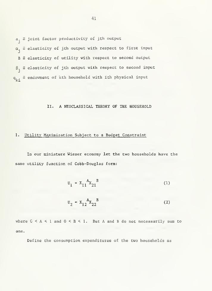
a. ^ joint factor productivity of j th output
a. = elasticity of jth output with respect to first input
B = elasticity of utility with respect to second output
3. = elasticity of jth output with respect to second input
q, E endowment of kth household with ith physical inputki
II. A NEOCLASSICAL THEORY OF THE HOUSEHOLD
1. Utility Maximization Subject to a Budget Constraint
In our miniature Wieser economy let the two households have the
same utility function of Cobb-Douglas form:
"i = ^uXi' ('>
"2 - '=12%2' <2>
where C < A < 1 and < B < 1. But A and B do not necessarily sum to
one.
Define the consumption expenditures of the two households as
42
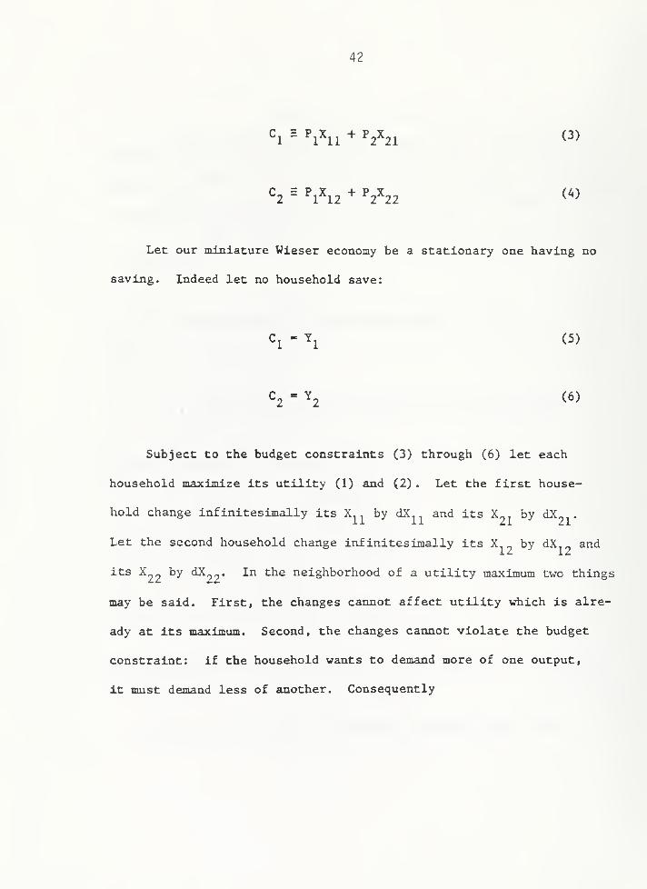
Cj H PjXjj + PjXjj (3)
C3 E PjXj2 + P^X^j (M
Let our miniature Wieser economy be a stationary one having no
saving. Indeed let no household save:
Cj - Y^ (5)
C2 •= ^2 ^^^
Subject to the budget constraints (3) through (6) let each
household maximize its utility (1) and (2) . Let the first house-
hold change infinitesimally its X by dX and its X by dX .
Let the second household change infinitesimally its X _ by dX. ^ and
its X by <iX-^. In the neighborhood of a utility maximum two things
may be said. First, the changes cannot affect utility which is alre-
ady at its maximum. Second, the changes cannot violate the budget
constraint: if the household wants to demand more of one output,
it must demand less of another. Consequently
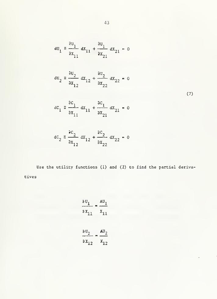
(7)
43
au 3UdU E —i^ dx +—i- dX,, «=
dU = dX,- + —^ dX^^ -
^^12 ^^22
3C 8CdC^ = —— dX^^ + —i^ dX^^ =
^^11 ^^21
3C 3CdC = —^ dX, - + —^ dX_, =
^^12 ^^22
Use the utility functions (1) and (2) to find the partial deriva-
tives
3 Uj^ AUj^
^^11 ^11
3Xj^2 ^12

44
^^1 ^1
3 U2 BU2
^^22 h.2
Use the budget definitions (3) and (4) to find the partial de-
rivatives
3C, 8C= P
^^11 ^^12
8C 3C= = P2
ax^j 3x^2
Insert these eight partial derivatives into the system (7) . Use
the latter to express the two marginal rates of substitution dX. ./dX-^
and dX^.J^j^, divide U, and U2 away, rearrange, and find
^2^21 " ^^1^11 ^^^

45
APjXjj - BP,Xj2 (9)
Insert (5) and (6) into (3) and (4), respectively, and write the two
budget constraints
^2 - Vl2 ^ ^2^22 (11>
Insert (8) sind (9) into (10) and (11), respectively, and write the
four demand functions
A YX^^ i (12)^^ A + B Pj^
A Y^
^^ A + B Pj^
B Y
X., (14)^^ A + B P2
46
B Y
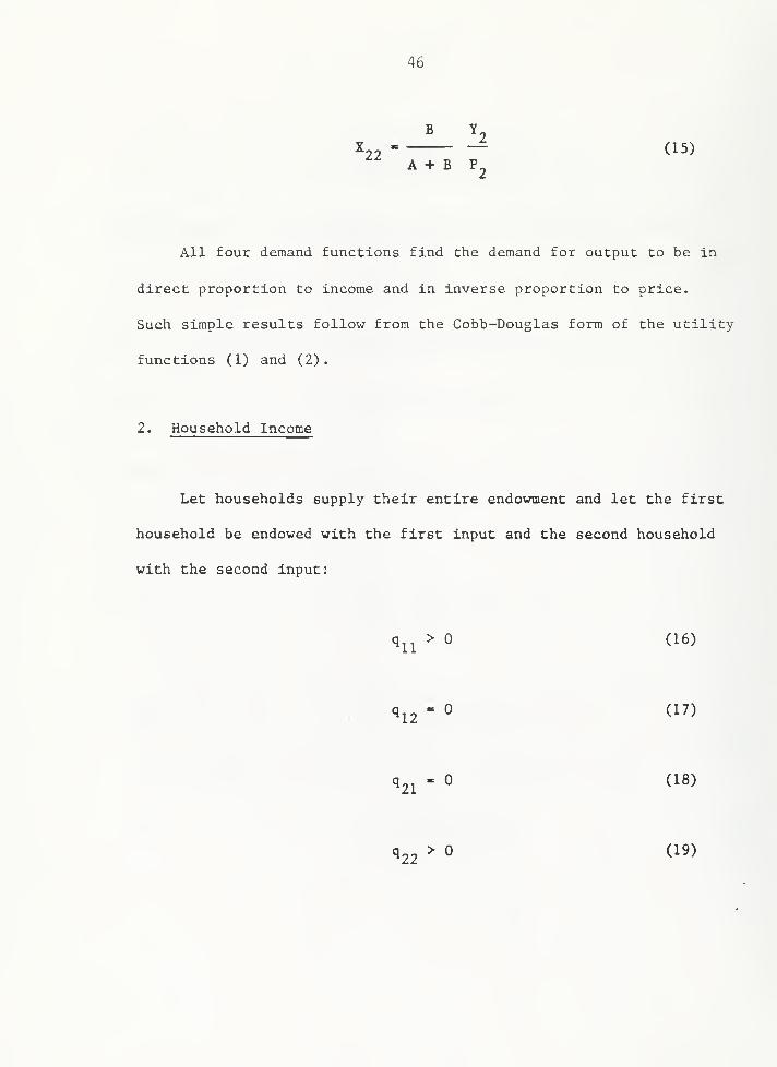
X22 (15)A + B P2
All four demand functions find the demand for output to be in
direct proportion to income and in inverse proportion to price.
Such simple results follow from the Cobb-Douglas form of the utility
functions (1) and (2).
2. Household Income
Let households supply their entire endowment and let the first
household be endowed with the first input and the second household
with the second input:
q^^> (16)
qi2" ° (^^)
q^j^- (18)
^22 ^ (1^)
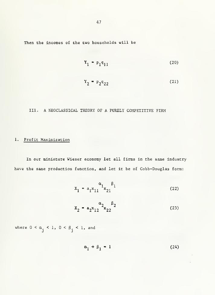
47
Then the incomes of the two households will be
^1 - Pjqii (20)
^2 " ^2^22 ^^^^
III. A NEOCLASSICAL THEORY OF A PURELY COMPETITIVE FIRM
1. Profit Maximization
In our miniature Wieser economy let all firms in the same industry
have the same production function, and let it be of Cobb-Douglas form:
^1 ^1^1 " ^^11 ^21 (22)
°2 h^2 " *2^12 ^22 (^"^^
where 0<a. <1, 0<3.<1, and
otj + ^1 - 1 (2A)

48
a^ + ^2 - 1 (25)
The cost of a representative firm is
^1 ~ Pl^ll "^ ^2^21 ^^^-^
^2 " ^1^12 "'' ^2^22 ^^^^
The revenue of a representative firm is
R^ = P^X^ (28)
R2 = ^2^2 ^^^^
The profits of a representative firm is
^1 ~ ^1 " ^1 ^^°^
^2 ~ ^2 ~ ^2 ^-^^^
and will be maximized with respect to inputs;

49
8Z 3X.—^ - ^1—^ - Pi -
3Z 3X.
3Z 3X
3x^2 3^12
3Z 3X
7^ "^27^-^2"°3x^2 3x22
Use the production functions (22) and (23) to find the four
partial derivatives, rearrange, and write the four demand functions
x^^ - a^P^X^/p^ (32)
^12 " °^2^2^2^Pl ^^^^
-21 - ^I'lh^^l <3^)
50
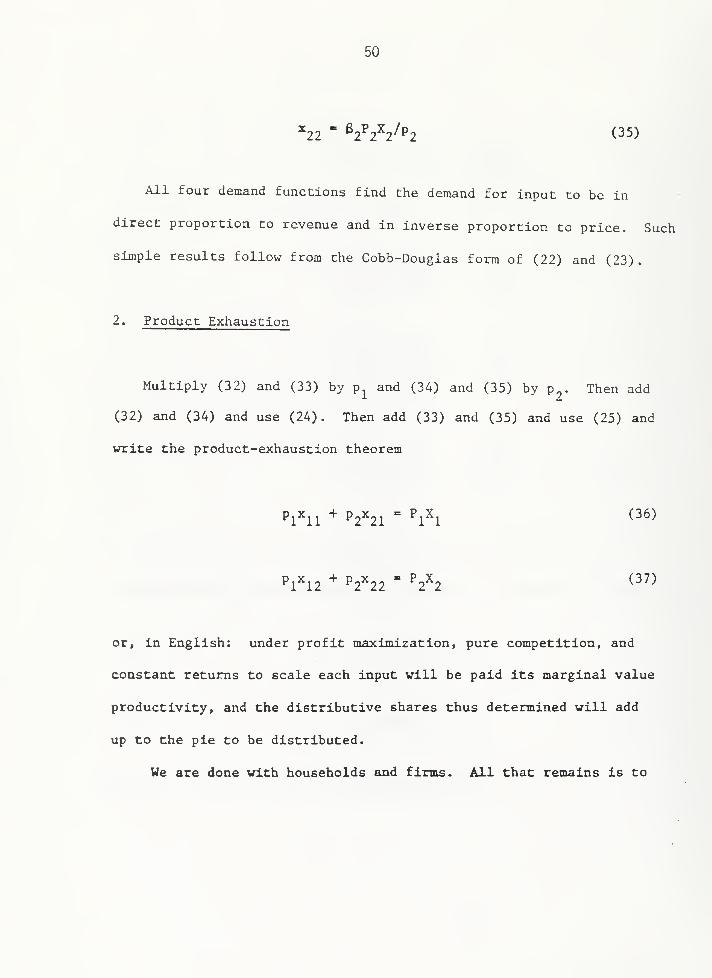
^22 = 62P2X2/P2 (35)
All four demand functions find the demand for input to be in
direct proportion to revenue and in inverse proportion to price. Such
simple results follow from the Cobb-Douglas form of (22) and (23).
2. Product Exhaustion
Multiply (32) and (33) by p^ and (34) and (35) by p . Then add
(32) and (34) and use (24). Then add (33) and (35) and use (25) and
write the product-exhaustion theorem
^1^11 '*' ^2^21 " ^1^1 ^^^^
Pl^2 "^l^^ll
= ^2^2 (3^)
or, in English; under profit maximization, pure competition, and
constant returns to scale each input will be paid its marginal value
productivity, and the distributive shares thus determined will add
up to the pie to be distributed.
We are done with households and firms. All that remains is to
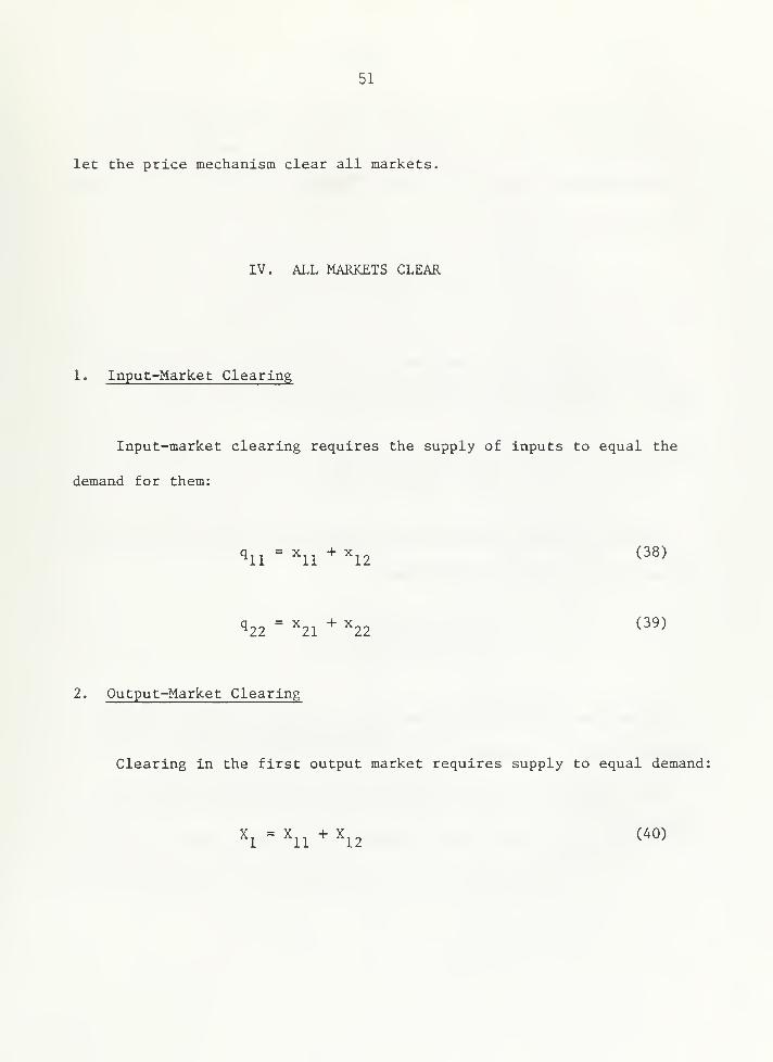
51
let the price mechanism clear all markets.
IV. ALL MARKETS CLEAR
1. Input-Market Clearing
Input-market clearing requires the supply of inputs to equal the
demand for them:
^11 = ^11 -^ ^2 (^^>
^22 = ^21 ^ ^22 (3^)
2. Output-Market Clearing
Clearing in the first output market requires supply to equal demand;
X^ = X^^ + X^2 (^°>
52
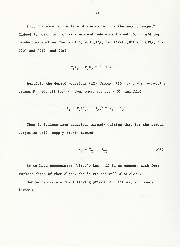
Must the same not be true of the market for the second output?
Indeed It must, but not as a new and independent condition. Add the
product-exhaustion theorem (36) and (37), use first (38) and (39), then
(20) and (21), and find
P,X, + P^X^ '\^^2
Multiply the demand equations (12) through (15) by their respective
prices P., add all four of chem together, use (40), and find
P^X^ + P^CX^, * X^j) -T(i + Y^
Thus it follows from equations already written that for the second
output as well, supply equals demand:
^2 " ^1 *" hi ^^^^
So we have encountered Walras's Law: if in an economy with four
markets three of them clear, the fourth one will also clear.
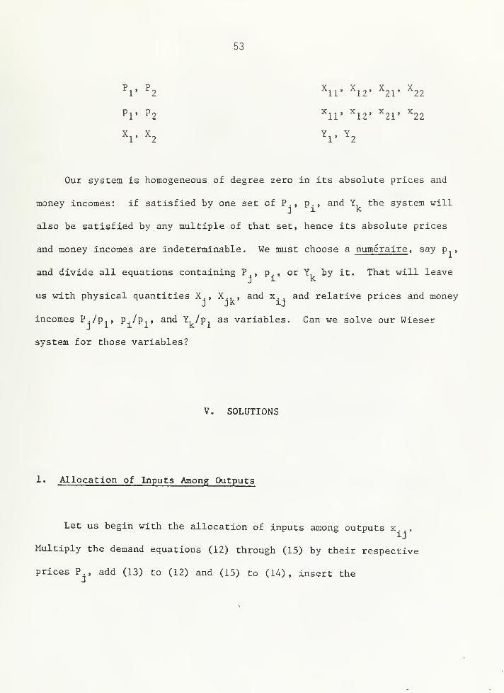
Our variables are the following prices, quantities, and money
Incomes:
53
^1' ^2 ^ir ^12' ^21' ^22
Pi' ^2 ^11' ""12' "^21' ""22
X^, X^ Y^, Y^
Our system is homogeneous of degree zero in its absolute prices and
money incomes: if satisfied by one set of P., p., and Y, the system will
also be satisfied by any multiple of that set, hence its absolute prices
and money incomes are indeterminable. We must choose a numeraire, say p ,
and divide all equations containing P., p., or Y, by it. That will leave
us with physical quantities X., X., , and x.. and relative prices and money
incomes P. /p., p./p,, and Y,/p. as variables. Can we solve our Wieser
system for those variables?
V. SOLUTIONS
1. Allocation of Inputs Among Outputs
Let us begin with the allocation of inputs among outputs x...
Multiply the demand equations (12) through (15) by their respective
prices P^ , add (13) to (12) and (15) to (14), insert the

54
output-market clearing conditions (40) and (41) and the product-exhaustion
theorems (36) and (37), and find A(p x _ + P2X22) = ^^Pi^n "^ P2'^21^ *
Next divide (32) by (34) and find P,x = (a /3,)P2X2i- Divide (33) by
(35) and find P,x._ = (a„/3^)p^x _. Insert all that, apply the result
to the input-market clearing conditions (38) and (39) , and find the so-
lutions for the allocation of inputs among outputs:
a, A + a2B
*12 ^11a, A + a-B
^21 ^22B^A + 62B
X . '2' q,, W)*22 ^22
B^A + B^'R
Once we are this far, the rest is easy.
55
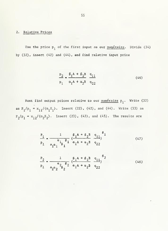
2. Relative Prices
Use the price p^ of the first input as our numeraire . Divide (34)
by (32) , insert (42) and (44) , and find relative input price
p 3, A + B„B q_£ - —
i
f- -^ (46)
p^ a^A + a^B q22
Next find output prices relative to our numeraire p. . Write (32)
as P./P, = X /(a X ). Insert (22), (42), and (44). Write (33) as
P /p = X /(a X^). Insert (23), (43), and (45). The results are
Pi a^a^ '6/ -lA^ V ^22
Po i ^lA + 6,B q ^2
-^ ' 5—T- (-^^ ^ —
>
<^8)

56
3. Outputs
Simply Insert the solutions (42) through (45) for the allocation
of Inputs among outputs into the production functions (22) and (23) and
find the solutions for outputs:
X, - a (^ ^^
) (^ ^^
) (49)
a Bq °2 62Bq22 ^2
X. - a (^ -^^
)(-Ji—if_) (50)
a,A + a2B Bj^A + B2B
A. Allocation of Outputs Among Households
Insert (20) and (42) into (12) and find X . Insert (21), (46)
,
and (47) into (13) and find X . Insert (20) and (48) into (14) and
find X^,. Insert (21), (46), and (48) into (15) and find X . Then
the allocation of output among households is
A a 3^ VIV ^22/1
^^ A+ B ' ' e^A + 32Bq^i

57
<x^ &^ e^A + B^B q^^ 1
""i^-TTTVi ^1 ^77TT7 7~^ '22 <52)A + o a, A + a^D q~~
6oB a, Bj a, A + a^B q^^ 2
X,, a,a. ^6, (-^*^ —) qn (53)A + B ^ "^ ^ 6^A + 62^ ^11
a^ 82 B-j^A + 62Bqj^j^
2
^22-7—7^2 22 ^"7777 7"^ '22 <5'^>A + B a, A + a-B q22
5. Income Distribution
Divide (20) by p.. Divide (21) by p and insert (46). Then money
incomes relative to the numeraire p are
^1
Pi^11 (55)
Y2 6jA + BpB— - — ~ q, 1 (56)Pj^ a^A + a2B

58
VI. SUMMARY AND CONCLUSION
We have solved our stylized Wieser model for all its variables.
A solution is an equation having a variable on its left-hand side and
nothing but parameters on its right-hand side. Our solutions contained
four categories of parameters. First, engineering delivered the technolo-
gy parameters a. and B . • Second, tastes delivered the preference parame-
ters A and B. Third, nature delivered the resource parameters q, . > andK. jL
fourth, legal institutions established private ownership to resources, en-
abling private persons to earn an income from them.
As for price theory we can accept neither Smith's nor Wieser 's
one-way causal relationships between goods price and factor prices.
Goods price is not caused by factor prices as Smith thought. Factor
prices are not caused by goods price as Wieser thought. Instead,
we must insist, goods prices and factor prices are simultaneously
determined within a general-equilibrium model using technology,
preferences, resources, and legal institutions for its parameters.
Such functional interdependence was beyond Smith and Wieser
but not beyond Walras. But even Walras failed to prove the existence
of his general equilibrium. Such proof was first offered by
von Neumann to whom we now turn.
59
REFERENCES
C. Menger, Grundsatze der Volksvirthschaf tslehre , Vienna, 1871,
reprinted by the London School of Economics and Political Science,
1934, translated as Principles of Economics by and edited by J.
Dingwall and B. F. Hoselitz with an introduction by F. H. Knight,
Glencoe, 111., 1950,
F. von Wieser, Ursprung und Hauptgesetze des wirtschaf tlichen Werthes,
Vienna, 1884.
, Der naturliche Werth, Vienna, 1889, translated as Natural Value
by C. A. Malloch and edited with a preface and analysis by W. Smart,
Glasgow, 1893, reprinted New York, 1930.

60
Copyright Johns Eopkins University Press
CHAPTER 3
dynamics: existence of general equilibrium
Ahstract
Wieser and Walras considered stationary states and believed hut
never proved general eqtdlibria to exist. Cassel was the first to
consider a general equilibrium of a growing economy but still failed
to prove its ezn^stenae. The first to prove it was John von Neumann,
Von Neumann's proof used inequalities, A primal problem was to
find the highest rate of growth satisfying the inequality thiot for
every good current input absorbed must be less than or equal to cur-
rent output supplied, A dual problem was to find tJie lowest rate of
interest satisfying the inequality that in every process cost at time
t with interest added must he greater than or equal to revenue at time
t + 1. A saddle point would exist at which the maximized rate of
growth equaled the minimized rate of interest. The chapter will
build and solve a von Neumann model of two goods and tuio processes.
K
61
I. INTRODUCTION
1. Time, Place, and Problem
The late nineteenth century had seen two Vienna breakthroughs,
one in surgery by Billroth (1819-1894) and one in economics by Carl
Menger (1840-1921) . The early twentieth century saw a third break-
through, logical positivism, by Wittgenstein (1889-1951). Inspired
by logical positivism, Kurt Godel, Karl Menger (son of Carl Menger),
John von Neumann, Karl Schlesinger, Abraham Wald, and other mathema-
ticians met in a colloquium that happened to devote some of its time
to the very foundation of economic theory: did a general economic
equilibrium exist?
Walras [1874-1877 (1954: 43-44)] considered general equilibrium
to be determinate "in the sense that the number of equations entailed
is equal to the number of unknowns." As pointed out by Karl Menger
(1971: 50), for the next sixty years Walras' s belief remained un-
questioned. Neither uniqueness nor feasibility was ever discussed.
The form of general equilibrium best known to the members of
the colloquium was Cassel's [1918 (1932: 32-41 and 152-155)] dyna-
62
mization of it, "the uniformly progressing state". Like Walras,
Cassel failed to prove the existence of a solution.
2. Von Neumann* s Breakthrough
Such innocence lasted until the 1930s. In the Viennese colloquium
von Neumann [1937 (1945-1946)] formulated a balanced and steady-state
growth of a general equilibrium and proved the existence of a solution.
The model was slow in reaching print. According to Weintraub (1983:
13n) , recollections by Jacob Marschak suggest its genesis to be roughly
contemporary with von Neumann's early work on game theory (1928). The
model was presented orally to a Princeton mathematics seminar in 1932.
What was new was not the subject matter. The subject matter was
allocation and relative price, the heartland of micro theory. There was
substitution in both production and consumption. The model could "handle
capital goods without fuss and bother," as Dorfman-Samuelson-Solow
(1958) put it. There was explicit optimization in the model: its solu-
tions would weed out all but the most profitable process or processes.
There were free and economic goods: the solutions would tell us which
goods would be free and which economic.
63
What was new was method rather than subject matter. This time,
the matter was in the hands of mathematicians from the very beginning,
and the mathematics deployed was very different from the calculus
deployed after 1870. The maxima and minima were handled without the
use of any calculus at all. What von Neumann taught us was to use
Inequalities to formulate a primal and a dual problem. What von
Neumann offered was a solution of his primal and dual problem
displaying a saddle point.
We must convey the flavor of von Neumann's method. But being one
of the foremost mathematicians of the twentieth century, von Neumann
used nonelementary algebra. Can the von Neumann model be solved by
elementary algebra? If collapsed into two goods and two processes,
it can, and let its notation be as follows.
3. Variables
g = proportionate rate of growth
P . i price of ith good
p E relative price
r E rate of interest
64
u. = excess supply of ith good
V. = loss margin of jth process
X. = level of ith processJ
X = relative process level
4. Parameters
a. . = input of ith good absorbed per unit of jth process level
b. . = output of ith good supplied per unit of jth process level
II. THE MODEL
1 . Goods and Processes
A von Neumann good may be absorbed as an input as well as supplied
as an output. A von Neumann process may have several inputs and several
outputs, and its unit level is defined as the unit of one of its outputs
per unit of time.
Let there be two goods, i = 1,2, and two processes, j = 1,2. Ope-
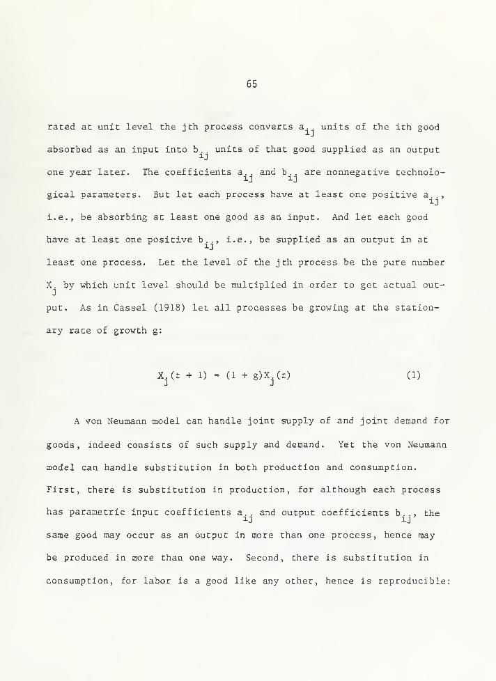
65
rated at unit level the jth process converts a., units of the ith good
absorbed as an input into b.. units of that good supplied as an output
one year later. The coefficients a., and b.. are nonnegative technolo-
gical parameters. But let each process have at least one positive a..,
i.e., be absorbing at least one good as an input. And let each good
have at least one positive b.., i.e., be supplied as an output in at
least one process. Let the level of the jth process be the pure number
X. by which unit level should be multiplied in order to get actual out-
put. As in Cassel (1918) let all processes be growing at the station-
ary rate of growth g:
X^(t + 1) = (1 + g)X^(t) (1)
A von Neumann model can handle joint supply of and joint demand for
goods, Indeed consists of such supply and demand. Yet the von Neumann
model can handle substitution in both production and consumption.
First, there is substitution in production, for although each process
has parametric input coefficients a., and output coefficients b.., the
same good may occur as an output in more than one process, hence may
be produced in more than one way. Second, there is substitution in
consumption, for labor is a good like any other, hence is reproducible:

66
labor is simply the output of one or more processes whose inputs are
consumers' goods. Although each such process has parametric input
coefficients a., and output coefficients b.., labor may occur as an
output in more than one process, hence may be produced in more than one
way—by being fed, so to speak, alternative menus.
Does the von Neumann model have capital in it? It does, in fact
it incorporates the time element of production In a particularly
elegant way. In the von Neumann model all processes have a period of
production of one time unit, but this is less restrictive than it
sounds: as for circulating capital, if consumable wine has a period
of production of two years, simply define two distinct processes and
goods as follows. The first process absorbs zero-year-old wine and
supplies one-year-old wine; the second absorbs one-year-old wine and
supplies two-year-old wine. As for fixed capital, if the useful life
of machines is two years, again define two distinct processes and
goods. The first process absorbs zero-year-old machines and supplies
one-year-old machines; the second absorbs one-year-old machines and
supplies two-year old machines!
2. The Primal Problem: Maximize the Rate of Growth
Feasibility requires overall excess demand for the ith good
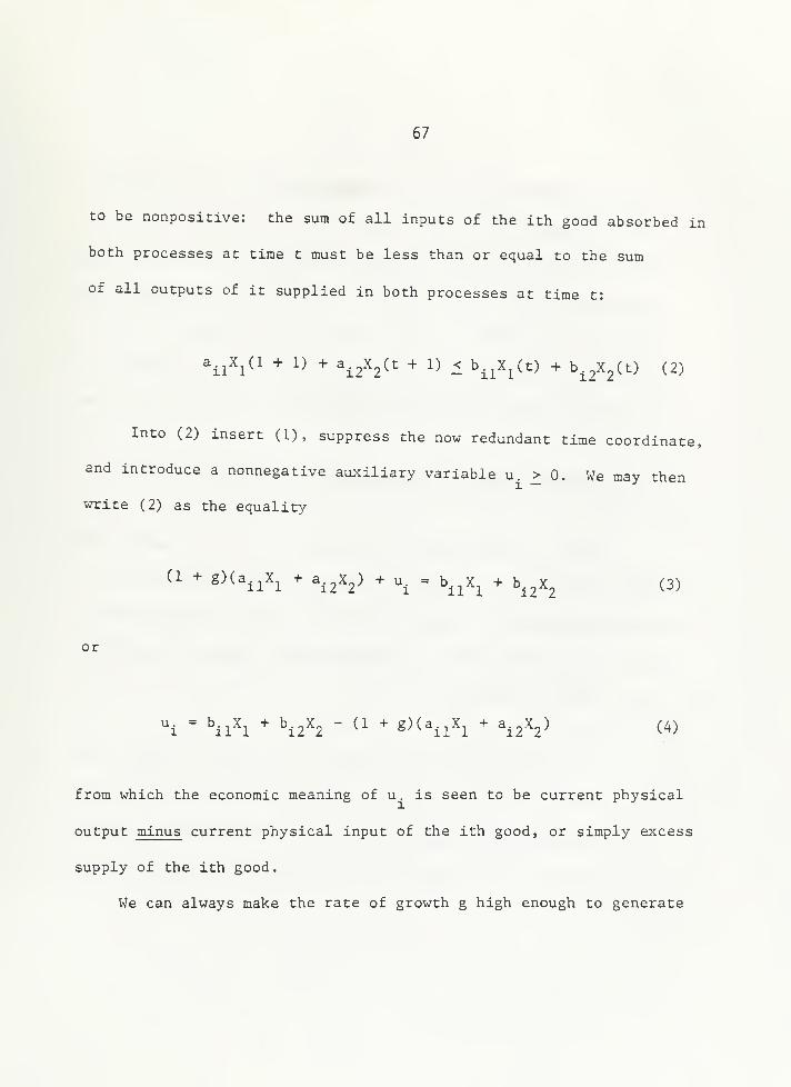
67
to be nonpositive; the sum of all inputs of the ith good absorbed in
both processes at time t must be less than or equal to the sum
of all outputs of it supplied in both processes at time t:
a.^X^d + 1) + a.^X^Ct + 1) < b.^X^(t) + b.^X^Ct) (2)
Into (2) insert (1), suppress the now redundant time coordinate,
and introduce a nonnegative auxiliary variable u. > 0. We may then
write (2) as the equality
(1 + g)(a,^X^ + a.^X^) + u. = b^^X^ + b.^X^ (3)
or
^ = hlh ^ ^12^2 - ^^ ^ S)(a,^X^ + a.^X^) (4)
from which the economic meaning of u. is seen to be current physical
output minus current physical input of the ith good, or simply excess
supply of the ith good.
We can always make the rate of growth g high enough to generate
68
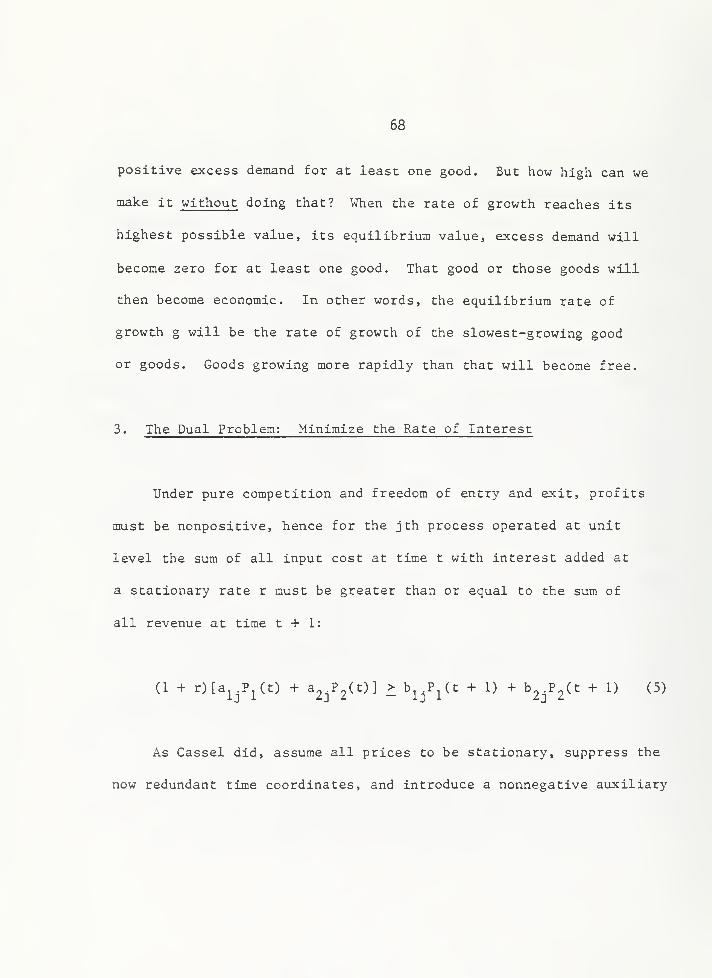
positive excess demand for at least one good. But how high can we
make it without doing that? When the rate of growth reaches its
highest possible value, its equilibrium value, excess demand will
become zero for at least one good. That good or those goods will
then become economic. In other words, the equilibrium rate of
growth g will be the rate of growth of the slowest-growing good
or goods. Goods growing more rapidly than that will become free.
3. The Dual Problem: Minimize the Rate of Interest
Under pure competition and freedom of entry and exit, profits
must be nonpositive, hence for the j th process operated at unit
level the sum of all input cost at time t with interest added at
a stationary rate r must be greater than or equal to the sum of
all revenue at time t + 1:
(1 + r)[a^^P^(t) + a^.?^(t)] > b^^P^(t + 1) + b^^P^Ct + 1) (5)
As Cassel did, assume all prices to be stationary, suppress the
now redundant time coordinates, and introduce a nonnegative auxiliary
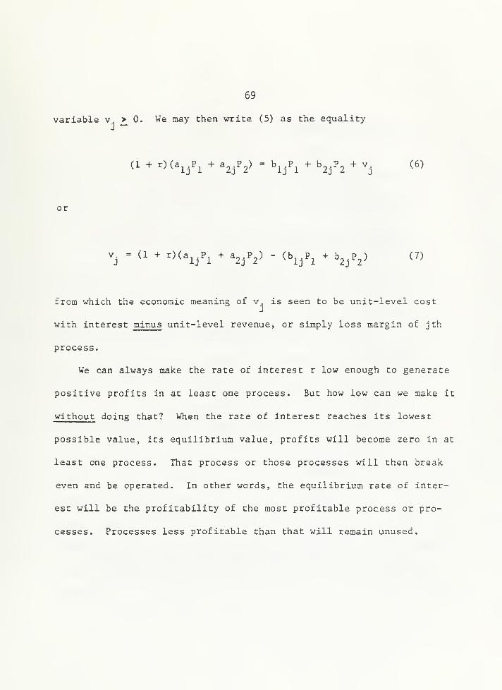
69
variable v. > 0. We may then write (5) as the equality
(l + DCa^.P^+a^jP^) - bj .P^ + byP^ + V. (6)
or
V. = (1 ^ r)(a^.P^ + a^.P^) - (b^.P^ * b^jP^) (7)
from which the economic meaning of v. is seen to be unit-level cost
with interest minus unit-level revenue, or simply loss margin of j th
process.
We can always make the rate of interest r low enough to generate
positive profits in at least one process. But how low can we make it
without doing that? When the rate of interest reaches its lowest
possible value, its equilibrium value, profits will become zero in at
least one process. That process or those processes will then break
even and be operated. In other words, the equilibrium rate of inter-
est will be the profitability of the most profitable process or pro-
cesses. Processes less profitable than that will remain unused.

70
4. The Saddle Point
Multiply the excess supply (4) of the ith good by its price P.
and write out the result for both goods 1=1, 2. Multiply the loss
margin (7) of the jth process by its level X. and write out the•J
result for both processes j = 1, 2. The four equations are
'l^'l " f^ll - ^1 ^ S^^ll^^l^l "^ f^l2 " ^^ "^ g)a^2JV2 (8)
^2^2 " ^^21 " ^^ "^ g)a23^]P2X^ + [h^^ - (1 + g)a22]P2^2 ^'^^
v^X^ = [(1 + r)a^^ - b^JP^X^ + [d + Oa^^ - b2jP2X^ (10)
V2X2 = [(1 + r)a^2 " ^12^^1^2 "*" ^^^ "^ ^''^22 " ^22^^2^2 *^^^^
Add (8) through (11):
P^u^ -H P2U2 + v^X^ + V2X2 =
(r - gXa^^P^X^ + a^2^^2 + ^21^2^1 + ^22^2V (12)
71
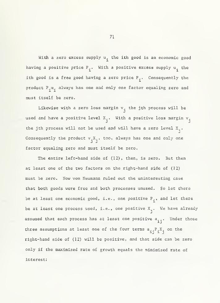
With a zero excess supply u. the ith good is an economic good
having a positive price P.. With a positive excess supply u. the
ith good is a free good having a zero price P.. Consequently the
product P.u. always has one and only one factor equaling zero and
must itself be zero.
Likewise with a zero loss margin v. the jth process will be
used and have a positive level X.. With a positive loss margin v.3 J
the ith process will not be used and will have a zero level X..J
Consequently the product v.X., too, always has one and only one
factor equaling zero and must itself be zero.
The entire left-hand side of (12), then, is zero. But then
at least one of the two factors on the right-hand side of (12)
must be zero. Now von Neumann ruled out the uninteresting case
that both goods were free and both processes unused. So let there
be at least one economic good, i.e., one positive P., and let there
be at least one process used, i.e., one positive X.. We have already
assumed that each process has at least one positive a... Under thoseij
three assumptions at least one of the four terms a..P.X. on the
right-hand side of (12) will be positive, and that side can be zero
only if the maximized rate of growth equals the minimized rate of
interest:

72
g = r
Such a saddle point was the heart of the von Neumann model.
But before finding its coordinates let us be more explicit about its
finance than von Neumann was himself.
In a growing economy somebody must be saving. We may think of a
von Neumann model as having capitalists in it who are lending money
capital to the entrepreneurs to carry them over their one-time unit
period of production. At the rate of interest r, capitalists at
the beginning of that period lend the entrepreneurs the sum
a..P.X, + a,^P.X„ + a„.P-X, + a_-P„X„ financing the purchases of all
goods absorbed as inputs.
At the end of the period of production the value of aggregate
output will be b^^P^X^ + b^^^^^X^ + b2j^P2^1 "^ ^22^2^2* ^^^ '^^^ ^^
express it in two different ways. First, since the product P.u. always
has one and only one factor equaling zero, we may set (8) and (9)
equal to zero, then add them and find aggregate input to have grown
into aggregate output at the rate g. Second, since the product v.X.
always has one and only one factor equaling zero, we may set (10) and
(11) equal to zero, then add them and find aggregate input to have

73
grown into aggregate output at the rate r. But in our saddle
point the maximized rate of growth g equaled the minimized rate
of interest r. Consequently, out of their sales proceeds the en-
trepreneurs can pay back with interest the sum they borrowed from
the capitalists one time unit earlier.
Now we must find the coordinates of the saddle point.
5. A Quadratic in Relative Process Levels
There was at least one economic good, say the second: P > 0,
u_ = 0, and one process used, say the second: X^ > 0. We may then safely
define relative process levels x = 1L,/X^ and write (3) for both goods:
b X + b - u /X
l + g=-^^^ —^ (13)
a^^x + a^2
b X + b
1 + g =^^ — (14)
a2^x + 3^2
Setting the right-hand sides of (13) and (14) equal and multiplying
across will give us the quadratic
74
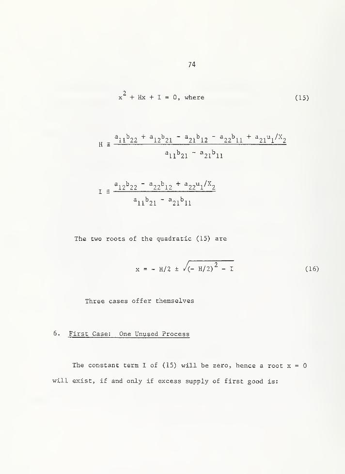
2X + Hx + I = 0, where (15)
_ ^11^21 -^ ^2^21 " ^21^2 ~ ^22^1 ^ ^Zl^l^^ZH = ————^^^^——^——^—.^^—^-^-^————^-^.^^^-^—^
^11^21 " ^21^11
^ . ^2^22 " ^22^2 ^ ^22^l/^2
^1^21 - ^21^1
The two roots of the quadratic (15) are
X = - H/2 ± /(- H/2)^ - I (16)
Three cases offer themselves
6. First Case: One Unused Process
The constant term I of (15) will be zero, hence a root x =
will exist, if and only if excess supply of first good is:
75
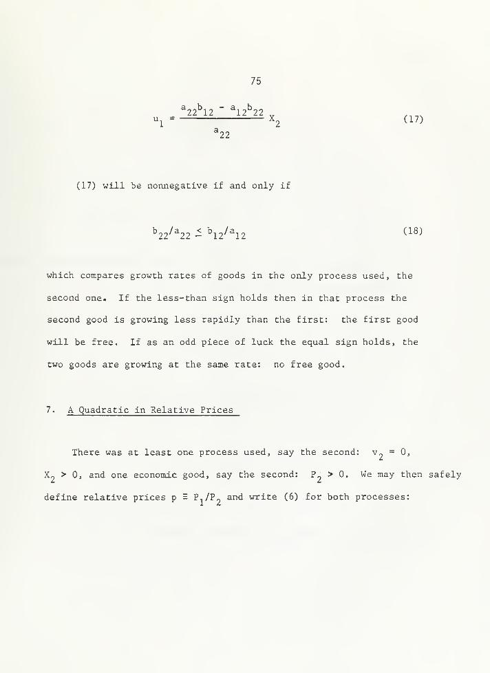
u^ = X^ (17)
^22
(17) will be nonnegative if and only if
^22/^22^^2/^2 (^^)
which compares growth rates of goods in the only process used, the
second one. If the less-than sign holds then in that process the
second good is growing less rapidly than the first: the first good
will be free. If as an odd piece of luck the equal sign holds, the
two goods are growing at the same rate: no free good.
7. A Quadratic in Relative Prices
There was at least one process used, say the second: v„ = 0,
X« > 0, and one economic good, say the second: P- > 0. We may then safely
define relative prices p = Pi/^o and write (6) for both processes:
76
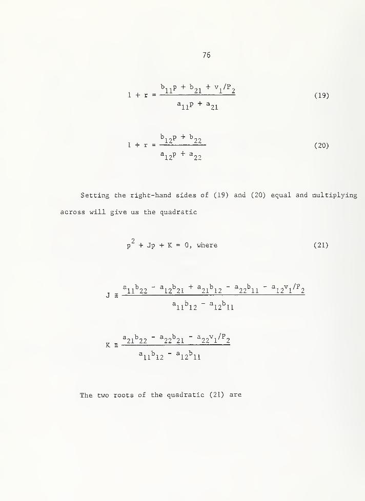
b p + b + V /P
1 + r = -^ —-(19)
1 + r = (20)
^2P + ^22
Setting the right-hand sides of (19) and (20) equal and multiplying
across will give us the quadratic
2p + Jp + K = 0, where (21)
^ . ^1^22 - ^2^21 -" ^21^2 - ^22^1 " ^2^l/^2
^1^2 - ^2^1
^ . ^21^22 " ^22^21 - ^22^l/^2
^1^12 - ^12^1
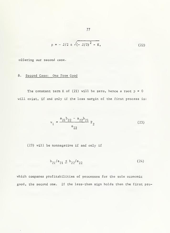
The two roots of the quadratic (21) are
77
P = - J/2 ± /(- J/2)^ - K, (22)
offering our second case.
8. Second Case: One Free Good
The constant term K of (21) will be zero, hence a root p =
will exist, if and only if the loss margin of the first process is;
^21^22 ^22^21 „
^22
(23) will be nonnegative if and only if
^2l''^21 - ^22^^22 ^^^-^
which compares profitabilities of processes for the sole economic
good, the second one. If the less-than sign holds then the first pro-
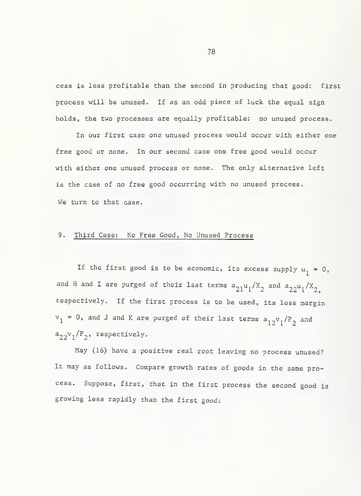
78
cess is less profitable than the second in producing that good: first
process will be unused. If as an odd piece of luck the equal sign
holds, the two processes are equally profitable: no unused process.
In our first case one unused process would occur with either one
free good or none. In our second case one free good would occur
with either one unused process or none. The only alternative left
is the case of no free good occurring with no unused process.
We turn to that case.
9. Third Case: No Free Good, No Unused Process
If the first good is to be economic, its excess supply u = 0,
and H and I are purged of their last terms a2l"l''^2 ^^^ ^22^1 ^^2
respectively. If the first process is to be used, its loss margin
v^ = 0, and J and K are purged of their last terms a v /P and
^22^l''^2'^^spectively.
May (16) have a positive real root leaving no process unused?
It may as follows. Compare growth rates of goods in the same pro-
cess. Suppose, first, that in the first process the second good is
growing less rapidly than the first good:
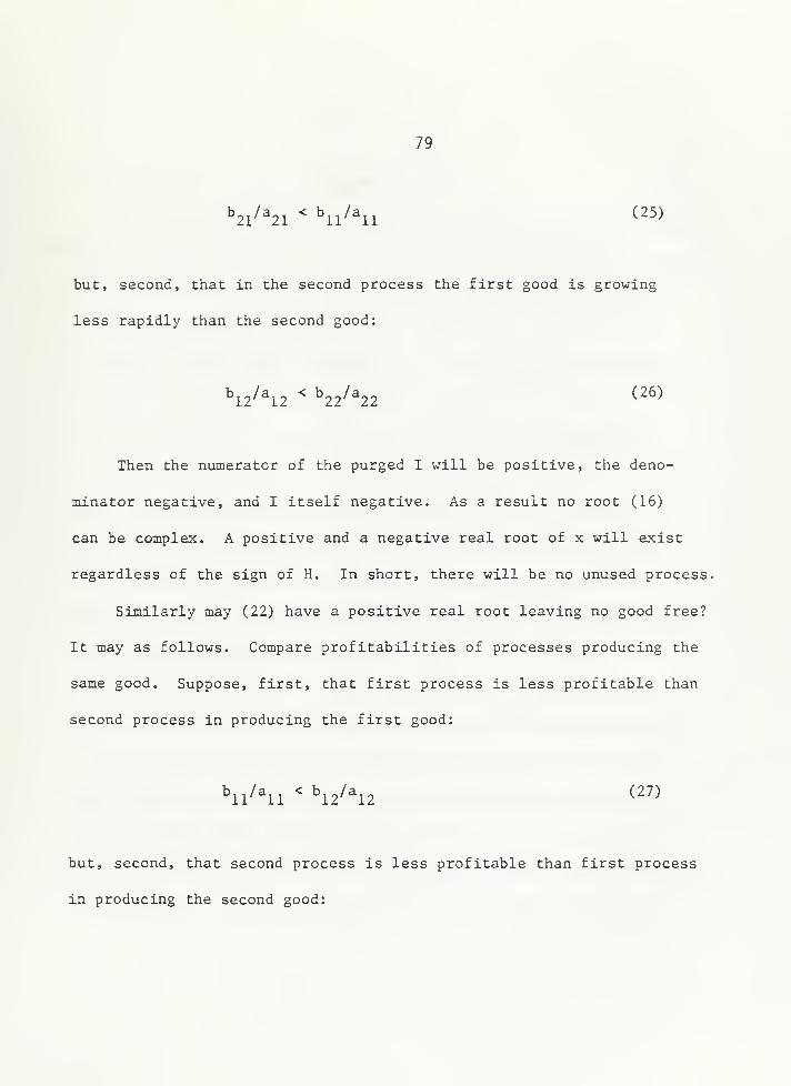
79
'=2l''^21-= "u/^l (")
but, second, that in the second process the first good is growing
less rapidly than the second good:
"12/^2 " "22/^22 (26)
Then the numerator of the purged I will be positive, the deno-
minator negative, and I itself negative. As a result no root (16)
can be complex. A positive and a negative real root of x will exist
regardless of the sign of H. In short, there will be no unused process.
Similarly may (22) have a positive real root leaving no good free?
It may as follows. Compare profitabilities of processes producing the
same good. Suppose, first, that first process is less profitable than
second process in producing the first good:
hi/^i ^ ^2/^2 ("'
but, second, that second process is less profitable than first process
in producing the second good:

80
b^^/ajj < b^^/a^j (28)
Then the numerator of the purged K will be negative, the deno-
minator positive, and K itself negative. As a result no root (22)
can be complex. A positive and a negative real root of p will exist
regardless of the sign of J. In short, there will be no free good.
10. Summary
Our (3) and (6) would remain satisfied if process levels X.,
prices P., excess supplies u., and loss margins v. were multiplied
by an arbitrary constant. Reduced to (3) and (6) , then, the von
Neumann system was homogenous of degree zero in its absolute pro-
cess levels, prices, excess supplies, and loss margins and could
only be solved for its relative ones. Since the numbering of goods
and processes is arbitrary, we assumed that at least the second
good would be economic and at least the second process be used.
In that case dividing by P„ or X^ would always be meaningful, and
the system could be solved for its relative process level x, its
relative price p, its relative excess supply u./X , and its re-

81
lative loss margin v./P^. Solving for those four coordinates of the
von Neumann saddle point we found three cases. May the cases coexist?
We notice at once that technologies satisfying (18) cannot sa-
tisfy (26) and vice versa: first and third case cannot coexist.
Similarly, technologies satisfying (24) cannot satisfy (28) and vice
versa: second and third case cannot coexist.
But could first and second case coexist with one another?
The answer is an easy yes if we ignore our odd pieces of luck,
the equal signs of (18) and (24) . Technologies may then exist sa-
tisfying the inequality parts of (18) and (24) at the same time.
As a result a homogenous (15) and a homogenous (21) may coexist
and have the roots x = and p = 0, respectively: one unused process
may coexist with one free good.
The answer is no if we cannot ignore our odd pieces of luck.
The equal sign of (18) would mean one unused process coexisting with
no free goods—ruling out the second case. The equal sign of (24)
would mean one free good coexisting with no unused process—ruling
out the first case.
In short, we may have, first, one unused process coexisting with
one free good, second, one unused process coexisting with no free

82
good, third, one free good coexisting with no unused process, and
fourth, no unused process coexisting with no free good. We have
discussed all four possibilities and specified the technologies
that would generate them.
11. Preferences ?
How did von Neumann treat consumption? Who consumed? Assuming
all his goods to be reproducible, von Neumann excluded natural resources
their owners, and Che consumption by such owners. Like Walrasian ones
von Neumann's entrepreneurs didn't consume anything, because their
income qua entrepreneurs was zero—pure competition and freedom of
entry and exit saw to that. Capitalists did have an interest
income but saved all of it. That left labor as the only
consumer in a von Neumann model. Labor was a good like any other,
hence was reproducible: labor was simply the output of one or more
processes whose inputs were consumers' goods. Labor might occur as an
output in more than one process and thus be produced in more than one
way—by being fed, so to speak, alternative menus. The alternative
menus did represent substitution in consumption, but how was the
83
choice among thera made? Labor-producing processes displaying zero
loss margins would be operated at positive levels representing the
consumption choice of the economy. But that choice did not express
anybody's preference; it merely minimized the cost, including
interest, of breeding labor. Labor was bred as cattle!
84
REFERENCES
G. Cassel, Theoretlsche Sozlalokonomle , Leipzig, 1918, translated as
The Theory of Social Economy by S. L. Barron, New York, 1932.
R. Dorfman, P. A. Samuelson, and R. M. Solow, Linear Programming and
Economic Analysis , New York, 1958, 381-388.
K. Menger, "Austrian Marginalism and Mathematical Economics," in J. R.
Hicks and W. Weber (eds.), Carl Menger and the Austrian School of
Economics , Vienna, 1971, 38-60.
J. von Neumann, "Ueber ein okonoraisches Gleichungssystera und eine
Verallgemeinerung des Brouwerschen Fixpunktsatzes,
" Ergebnisse
eines mathematischen Kolloquiums , 8, Leipzig and Vienna, 1937,
73-83, translated by G. Morgenstern (Morton) as "A Model of General
Economic Equilibrium," Rev. Econ. Stud. , 1945-19A6, L3, 1-9. "The
printing was terrible," says Weintraub (1983: 13n) , and "a number
of typographical errors have been corrected" by W. J. Bauraol and
S. M. Goldfeld (eds.). Precursors in Mathematical Economics; An
Anthology , London, 1968, 296-306.

85
L. Walras, Elements d'economle politique pure , Lausanne, Paris, and
Basle, 1874-1877, translated as Elements of Pure Economics or the
Theory of Social Wealth by W. Jaffe, Horaewood , 111., 1954.
E. R. Weintraub, "On the Existence of a Competitive Equilibrium:
1930-1954," J. Econ. Lit., Mar. 1983, 21, 1-39.

86
APPENDIX: A MATHEMATICAL REMINDER
87
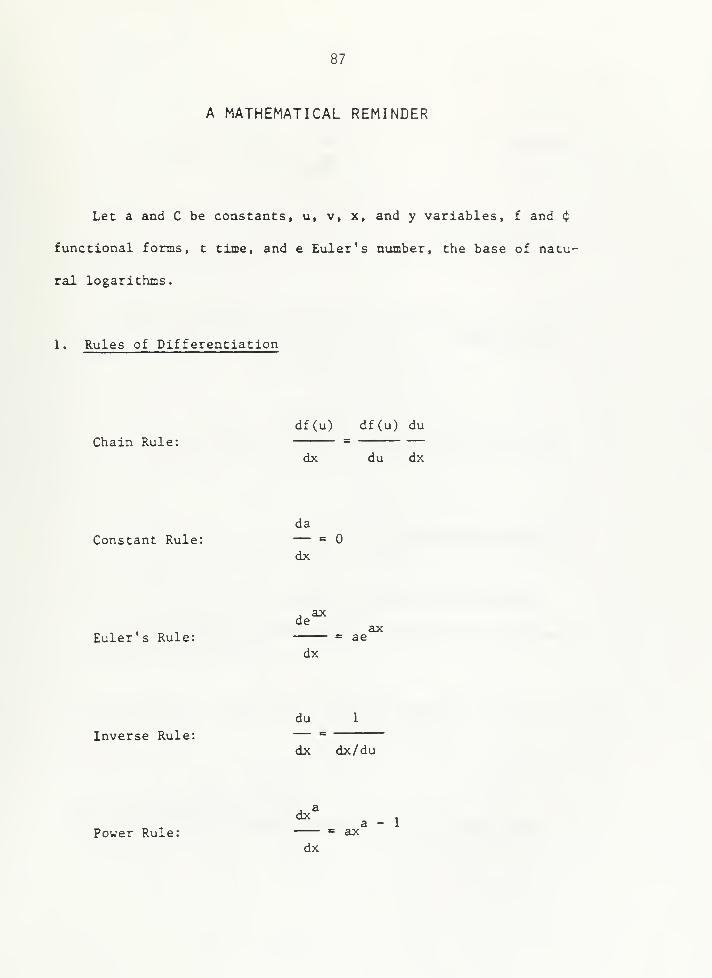
A MATHEMATICAL REMINDER
Let a and C be constants, u, v, x, and y variables, f and <$>
functional forms, t time, and e Euler's number, the base of natu-
ral logarithms.
1. Rules of Differentiation
df(u) df(u) du
Chain Rule:dx du dx
da
Constant Rule: — =
dx
de
Euler's Rule: = ae
dx
du 1
Inverse Rule:dx dx/du
dx ,a - 1
Power Rule: "= ax
dx

Product Rule:
Proportion Rule:
88
d(uv) dv du= u — + V —
dx dx dx
d(ax)= a
dx
d(u/v) v(du/dx) - u(dv/dx)Quotient Rule: = r-
dx V
d(u ± v) du dv
Sum or Difference Rule:
dx dx dx
2. Rule of Integration
The indefinite integral /f(x)dx of the integrand f(x) will
equal 4)(x) + C, where C is the constant of integration, if
d(^(x)
" f (x)
dx
From Euler's Rule of differentiation it then follows that
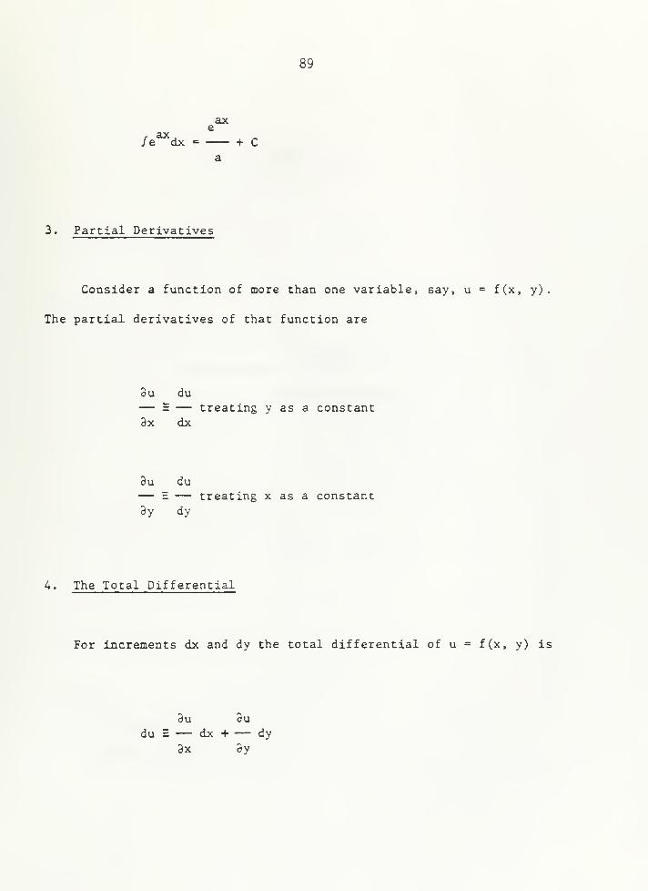
89
axe
/e^dx = + C
3. Partial Derivatives
Consider a function of more than one variable, say, u = f(x, y)
The partial derivatives of that function are
9u du— = — treating y as a constant3x dx
9u du— E — treating x as a constant
3y dy
4. The Total Differential
For increments dx and dy the total differential of u = f(x, y) is
8u 9u
du = — dx + — dy
3x 3y
90
INDEX
MICROECONOMICS

91
INDEX
MICROECONOMICS
Absolute prices, 53
Allocation
of inputs among outputs, 53-54
of outputs among households, 56-57
theory, 38
Budget constraint, household, 42
Cantillon, 10-14
Capital
circulating, 15
coefficients, 20

92
durability, 18, 19, 24
elasticity, 25
fixed, 18, 24
in von Neumann model, 66
Cassel , 61, 65, 68
Cobb-Douglas form, 25, 41, 46, 47, 50
Colloquium, mathematical, 61
Competition, pure, 26, 40, 47-50, 68
Constant returns to scale, 25, 40, 47, 48, 50
Cost, 12, 15, 48
Daal , van, 32

93
Demand for
factors, 26-27, 28
inputs, 49-50
outputs, 45-46
Differentiation, 87-89
Diminishing returns, 10, 20, 25
Discounting future cash flows, 19-20, 24-25
Distributive shares, 27, 50
Dorfman-Samuel son-Sol ow, 62
Dual problem, 63, 68-70
Economic goods, 60-83
94
EUis, 14
Endowment, 46
Equalization of rates of
profit, 21
surplus value, 21
Equilibrium. See Market clearing
Excess
demand, 66-68
supply, 67
Factor
prices, 30, 39, 55
use, 26-27, 28, 49-50
Free goods, 60-83

95
Freedom of entry and exit, 12, 15, 21, 68
Future cash flow, 19, 24
Game theory, 62
General equilibrium, 31, 37-59, 60-83
Goods and processes in von Neumann model, 64-66
Goods price, 30, 39, 55
Gordon, R. A., 23
Growth rate, 67-68, 71-72
Herberg, 32

96
Hollander, 14
Homogeneity of degree zero in
prices, 53, 80
process levels, 80
Household
budget, 42
income, 46-47
Imputation, 38-39
Income
distribution, 57
household, 46-47
Inequalities, 60, 63, 67-68
97
Input coefficients
Cantillon, 11
Marx, 20
Smith, 15
von Neumann, 65
Input elasticities, 25
Integration, 88-89
Interest rate, 23, 60, 69, 71-73
Joint factor productivity, 10, 41
Labor
bred as cattle, 83
98
demand for, 26
reproducible, 11, 16, 22, 65-66, 82-83
theory of value, 24, 30
Land, 11, 15, 20, 24
Land theory of value, 30
Legal institutions, 31, 58
Level of processes, 73-74
Loss margin, 69
Machinery, 18
Mai thus, 11, 22
Marginal productivity. See Physical marginal productivity

99
Market clearing, 51-53
Marx, 18-24
Maximization of
present net worth, 24-25
profits, 47-50
utility, 44-46
Menger,
Carl , 38
Karl , 61
Microeconomics, 4, 7-8
Multifactor productivity. See joint factor productivity
Natural price, 15-16

100
Nature, 58
Neoclassical theory of
firm, 47-51
household, 41-47
price, 24-29
Neumann, von, 11, 60-83
Niehans, 32
Numeraire, 53
One-way causal relationship
Smith, 30
Wieser, 39
Optimized labor, land, and capital stock, 26

101
Ott-Winkel, 21, 22
Output coefficients in von Neumann, 65
Parameters, 8-9, 58
Par between land and labor, 12
Partial derivatives, 89
Period of production, 15, 65, 66, 72
Physical marginal productivity of
capital stock, 26
labor, 26
land, 26
Prague, 39
102
Preferences, 31, 38, 58
Present net worth
Marx, 19-20
Neoclassicals, 24-25
Price
absolute, 53, 58
as equilibrating variable, 51-52
mechanism. See Price as equilibrating variable
natural , 15-16
of factors, 30, 39, 55
of goods, 30, 39, 55
relative, 8, 10-31, 53, 55, 75-77
"Prices" in Marx, 21
Primal problem, 63, 66-68
Private ownership to resources, 58
103
Processes
breaking even, 12, 13, 15, 68
Cantillon, 11
unused, 60-83
von Neumann, 64-66
Product exhaustion, 27, 50
Production function, 25, 47, 50. See also Technology
Profit maximization, 47-50
Pure competition, 26, 40, 47-50, 68
Quadratic in relative
prices, 75-77
process levels, 73-74

104
Rate of.
growth, 67-68, 71-72
interest, 23-24, 69, 71-73
profit, 21
surplus value, 21
Relative-price equation
Cantillon, 14
Marx, 22-23
neoclassical 27-28, 55
Smith, 17-18
von Neumann, 75-77
Relative-process-level equation, von Neumann, 73-74
Representative firm, 48
Resources, 31, 58
Ricardo, 18, 20
105
Saddle point, 70-73
Samuel son, 14, 18, 22
Saving, 72
Scale. See Constant returns to scale
Self-contained solution, 14, 30
Siven, 32
Smith, 3, 14-18
Solution, concept, 8-9. 58
Solutions for
general equilibrium, 53-57, 60-83
growth rate, 71-72
106
income distribution, 57
physical output, 56
rate of interest, 71-73
relative price, 30, 55, 75-77
relative process levels, 73-74
Stationary economy, 19, 25, 42
Subsistence minimum in
Cantillon, 11
Marx, 22
Smith, 16
Substitution, 28, 62, 65
Technology, 10, 14, 20, 25, 31, 58, 65
Total differential , 89

107
Total factor productivity. See Joint factor productivity
Trinity, Smith's, 15, 24
Turgot, 10
Uniformly progressing state, Cassel's, 61-62
Unused processes, 60-83
Utility
function, 41
maximization, 44-46
"Values" in Marx, 21
Variables, 8-9
108
Vienna, 61-62
Walras, 30, 58, 61
Walras's Law, 52
Weintraub, 62
Wicksell, 25
Wicksteed, 25, 27
Wieser, von, 39

109
ABOUT THE AUTHOR
Hans Brems is professor emeritus of economics at the University
of Illinois. Danish-born, he was naturalized in 1958. He has taught
at Copenhagen and Berkeley and, as a visiting professor, at Basle,
Copenhagen, Gothenburg, Gottingen, Hamburg, Kiel, Lund, Stockholm,
Uppsala, and Zurich. He has testified before the Joint Economic
Committee of the U.S. Congress. He is a foreign member of the Royal
Danish Academy of Sciences and Letters and of the Finnish Society of
Sciences.
His books include:
Product Equilibrium under Monopolistic Competition , Harvard, 1951
Output, Employment, Capital, and Growth , Harper, 1959; Greenwood, 1973
Quantitative Economic Theory , Wiley, 1968
Labor, Capital, and Growth, D. C. Heath, 1973
Inflation, Interest, and Growth , D. C. Heath, 1980
Dynamische Makrotheorie, J. C. B. Mohr (Paul Siebeck) , 1980
Fiscal Theory. D. C. Heath, 1983
Pioneering Economic Theory 1630-1980 , Johns Hopkins, 1986

no
END


HECKMANBINDERY INC.
JUN95in. , T PlciM?
N.MANCHESTER,Bound -To .PIcimT
i^idiai^a 46962


