
The Multiplier Model
Aggregate Expenditures and Aggregate Supply: The Short Run

Learning Objectives
• Understand how GDP is determined according to the logic of the multiplier model.
• Learn how to construct a graphical model.
• Know how to manipulate the components of the model to tell an economic story.
• Understand the multiplier process.

Income Determination
• The aggregate expenditure/aggregate supply model is designed to explain how the different sectors of the economy interact to determine the size and composition of GDP (Y) in the short run.
• The model is an equilibrium model.– Equilibrium is a state of rest where there are
either no forces causing change or equal opposing forces.
Equilibrium
• Equilibrium is achieved in the model when aggregate spending or expenditures just equal aggregate supply or output.– Aggregate expenditures = Aggregate Supply
AE AS

Aggregate Expenditures
• Aggregate expenditures are comprised of all spending done in the economy during a given period of time.– Aggregate expenditures are the sum of consumption
spending by the household sector, investment spending by businesses, government spending by all levels of government, and net exports.
• AE = C + I + G + (X-M)

Aggregate Supply• Aggregate supply is GDP. It is all final goods
and services produced during a given period of time.
AS = GDP or Y
• Aggregate supply is assumed to be perfectly responsive to spending.– Whenever expenditures change, aggregate supply
changes by an equal amount.
Aggregate Supply
AE
Y
AS
0
B
D
E
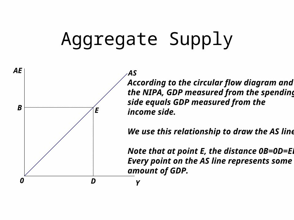
According to the circular flow diagram andthe NIPA, GDP measured from the spending side equals GDP measured from the income side.
We use this relationship to draw the AS line.
Note that at point E, the distance 0B=0D=ED.Every point on the AS line represents someamount of GDP.

Aggregate Supply• We depict aggregate supply graphically with a
ray from the origin.
• Every point on the ray represents GDP measured either from the expenditure side or from the income side.– GDP measured from the expenditure side is on the
vertical axis.
– GDP measured from the income side is on the horizontal axis.
• The AS line in this model NEVER moves.

Consumption Spending
• Consumption is defined as all spending done by the household sector on durables, non-durables, and services.
• Consumption is assumed to be determined primarily by disposable income (Yd), but it also may be affected by taxes, changes in the price level, and real wealth.
• C = a0 + bYd is the consumption function.
Consumption Function
C
Y
AS
0
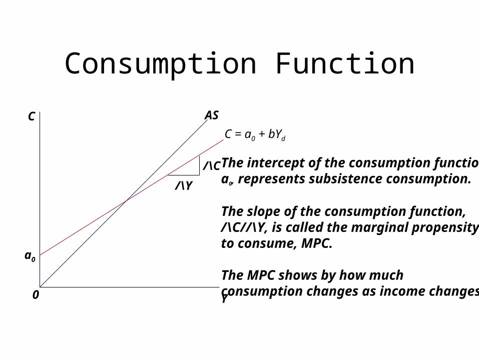
C = a0 + bYd
a0
/\Y
/\C The intercept of the consumption function,a0, represents subsistence consumption.
The slope of the consumption function,/\C//\Y, is called the marginal propensityto consume, MPC.
The MPC shows by how much consumption changes as income changes.
Consumption and Saving
Y1 Y2 Y3 Y
Y
S=-a + (1-b)Yd
C=a + bYd
AS
S0
0
-a
a
C
E
E
A
A’
B’
B
C’
C
D’
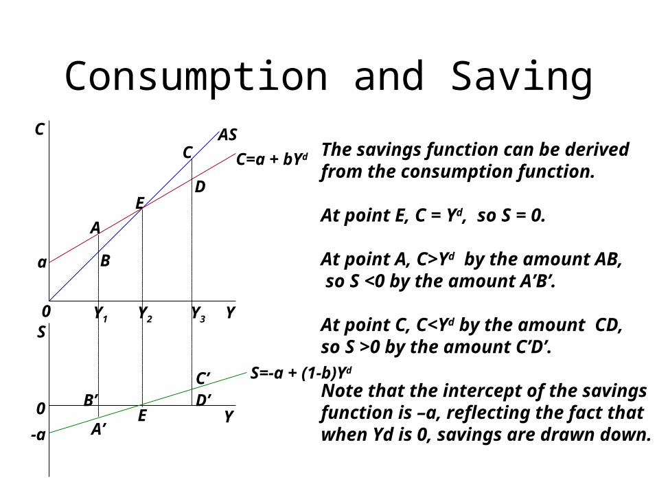
The savings function can be derivedfrom the consumption function.
At point E, C = Yd, so S = 0.
At point A, C>Yd by the amount AB, so S <0 by the amount A’B’.
At point C, C<Yd by the amount CD,so S >0 by the amount C’D’.
Note that the intercept of the savingsfunction is –a, reflecting the fact thatwhen Yd is 0, savings are drawn down.
D
Investment
• Investment is defined as all spending done by the business sector on plant, equipment, and inventories.
• An important determinant of investment spending is the rate of interest.– There is a negative relationship between
investment and the rate of interest.• As interest rates rise, investment falls.
• As interest rates fall, investment rises.
Interest Rates and Investment
• The negative relationship between interest rates and investment exists because firms must either borrow or generate their own funds to invest. – As a result, firms are willing to invest in only
those projects that pay a return in excess of the borrowing cost or rate of interest paid.
• When rates are high, few projects are sufficiently profitable, but as rates fall, more and more projects become profitable.
Investment and the Rate of Interest
r
Investment
I
i2
i1
I1 I2
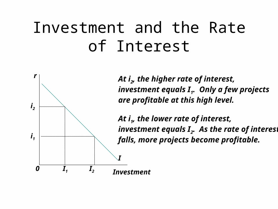
At i2, the higher rate of interest, investment equals I1. Only a few projectsare profitable at this high level.
At i1, the lower rate of interest,investment equals I2. As the rate of interestfalls, more projects become profitable.
0
Investment in the AE/AS Model
C+ I
Y
AS
0
C + I1 = AE1
C + I2 = AE2
Y1 Y2
B
A
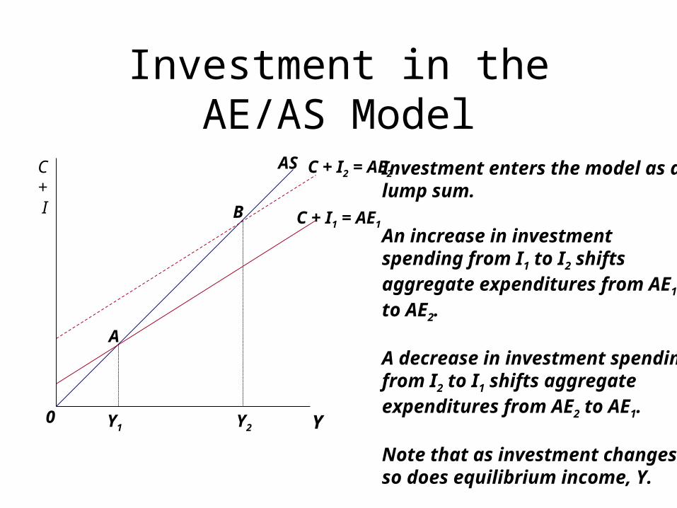
Investment enters the model as alump sum.
An increase in investmentspending from I1 to I2 shiftsaggregate expenditures from AE1
to AE2.
A decrease in investment spendingfrom I2 to I1 shifts aggregateexpenditures from AE2 to AE1.
Note that as investment changesso does equilibrium income, Y.
Saving and Investment
Y1 Y2 Y3 Y
Y
S
C
AS
S,I0
0
-a
a
C,I
E
E
C’
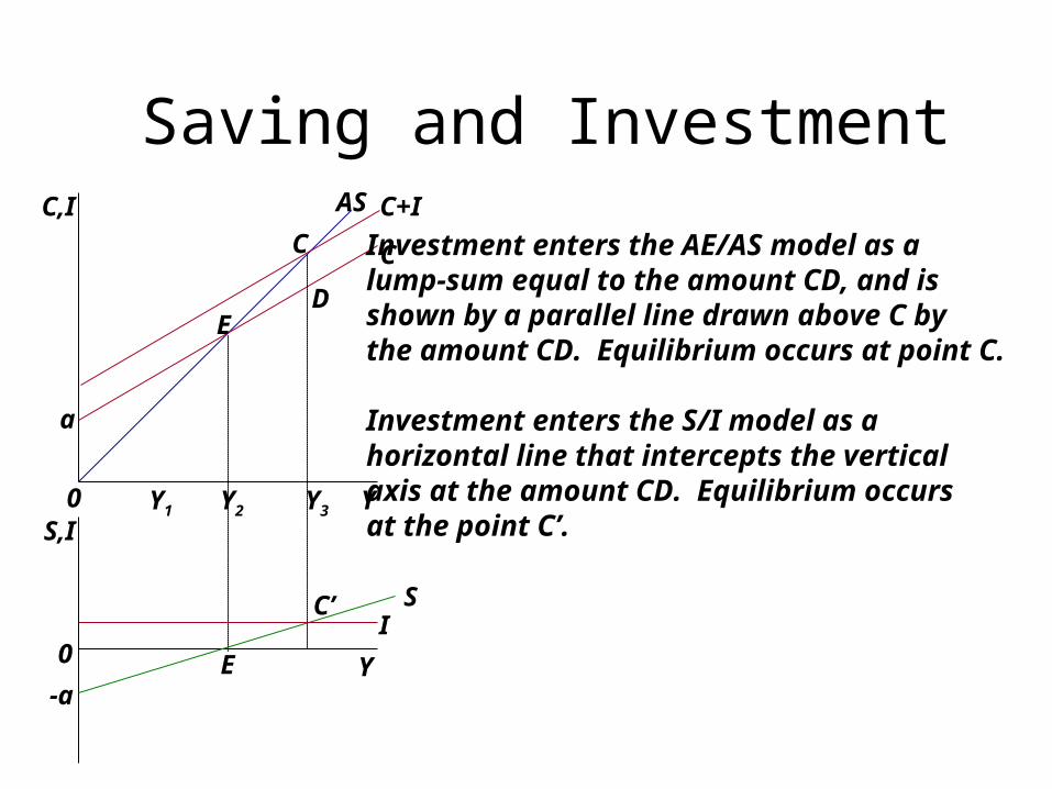
C Investment enters the AE/AS model as a lump-sum equal to the amount CD, and is shown by a parallel line drawn above C by the amount CD. Equilibrium occurs at point C.
Investment enters the S/I model as ahorizontal line that intercepts the verticalaxis at the amount CD. Equilibrium occursat the point C’.
D
C+I
I
Government Spending
• Government spending is defined as all spending done by all levels of government on goods and services.– Government spending enters the model as a lump-
sum.• We invoke this simplifying assumption because there is
no consistent relationship between government spending and the level of national income.

Government in the AE/AS Model
C + I +G
Y
AS
0
C
C+I
Y1
B
A
Government spending is drawn as a parallel line above C+I, reflecting theassumption that government spendingenters the model as a lump-sum.
The distance between C+I and C+I+Grepresents lump-sum government expenditures.
At Y1, consumption equals the linesegments Y1B, consumption plusinvestment is Y1A, consumptionplus investment plus governmentspending is Y1E, investment isAB, and government spending is AE.
C+I+G
E
Government in the AE/AS Model
• Changes in government spending cause the government line and, therefore, the aggregate expenditure line to shift.– Increases in government spending shift G and
therefore AE up.
– Decreases in government spending shift G and therefore AE down.
Government in the AE/AS Model
C + I +G
Y
AS
0
C+I+G1 = AE1
C+I+G3 = AE3
Y1 Y2 Y3
B
A
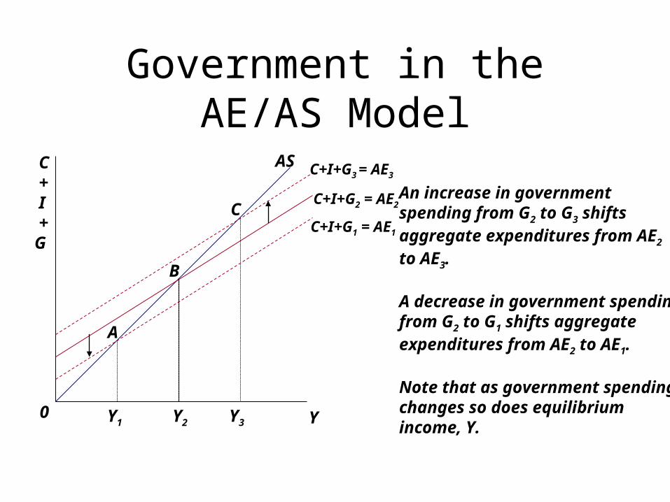
An increase in governmentspending from G2 to G3 shiftsaggregate expenditures from AE2
to AE3.
A decrease in government spendingfrom G2 to G1 shifts aggregateexpenditures from AE2 to AE1.
Note that as government spending changes so does equilibrium income, Y.
C+I+G2 = AE2C
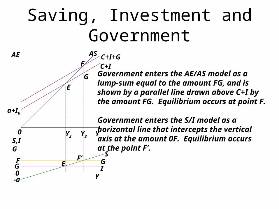
Saving, Investment and Government
Y2 Y3 Y
Y
S
C+I
AS
S,IG
0
0-a
AE
E
EF’
F
G
C+I+G
IG
a+I0
Government enters the AE/AS model as a lump-sum equal to the amount FG, and is shown by a parallel line drawn above C+I by the amount FG. Equilibrium occurs at point F.
Government enters the S/I model as ahorizontal line that intercepts the verticalaxis at the amount 0F. Equilibrium occursat the point F’.
FG

Practice
C
C + I
C + I + G
Y
AE
p
n
m
Y1 Y2 Y3
a
b
c
d
e
f
g
h
j
AS
0

Practice• Assume Y = Y1 and using vertical line segments
determine the following:– Consumption at Y1
– Investment at Y1
– Government spending at Y1
– Aggregate expenditures at Y1
– Consumption plus investment at Y1
– Investment plus government spending at Y1
• Repeat, assuming first that Y=Y2 and then Y=Y3

Net Exports
• Net exports are the difference between the goods and we produce for the rest of the world and the goods and services they produce for us.– Net exports equal exports minus imports
• NX = (X- M)
– Net exports enter the model as a lump sum.
Determinants of Net Exports
• Exports– Income in the rest of the world
• As income in the rest of the world increases (decreases), they buy more (less) from us.
– Relative prices• As our prices fall (rise) relative to prices in the rest of the
world, they buy more (less) from us.
– Exchange rate• As our currency appreciates (depreciates) relative to
other currencies, they buy less (more) from us.
Determinants of Net Exports
• Imports– Income at home in the domestic economy
• As domestic income increases (decreases), we buy more (less) from abroad.
– Relative prices• As our prices fall (rise) relative to prices in the rest of the
world, we buy less (more) from abroad.
– Exchange rate• As our currency appreciates (depreciates) relative to
other currencies, we buy more (less) from abroad.
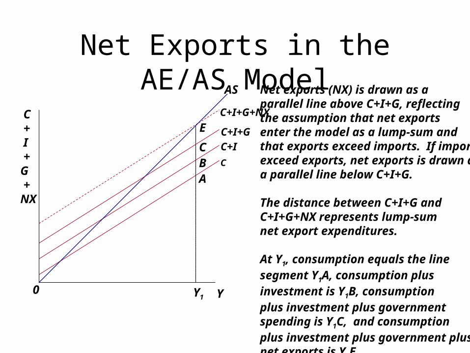
Net Exports in the AE/AS Model
C + I +G +NX
Y
AS
0
C
C+I
Y1
BA
Net exports (NX) is drawn as a parallel line above C+I+G, reflectingthe assumption that net exportsenter the model as a lump-sum andthat exports exceed imports. If importsexceed exports, net exports is drawn asa parallel line below C+I+G.
The distance between C+I+G andC+I+G+NX represents lump-sumnet export expenditures.
At Y1, consumption equals the linesegment Y1A, consumption plusinvestment is Y1B, consumptionplus investment plus governmentspending is Y1C, and consumptionplus investment plus government plusnet exports is Y1E.
C+I+GEC+I+G+NX
C

Net Exports in the AE/AS Model
• Changes in net exports cause the net exports line and, therefore, the aggregate expenditure line to shift.– Increases in net exports shift NX and AE up.
– Decreases in net exports shift NX and AE down.
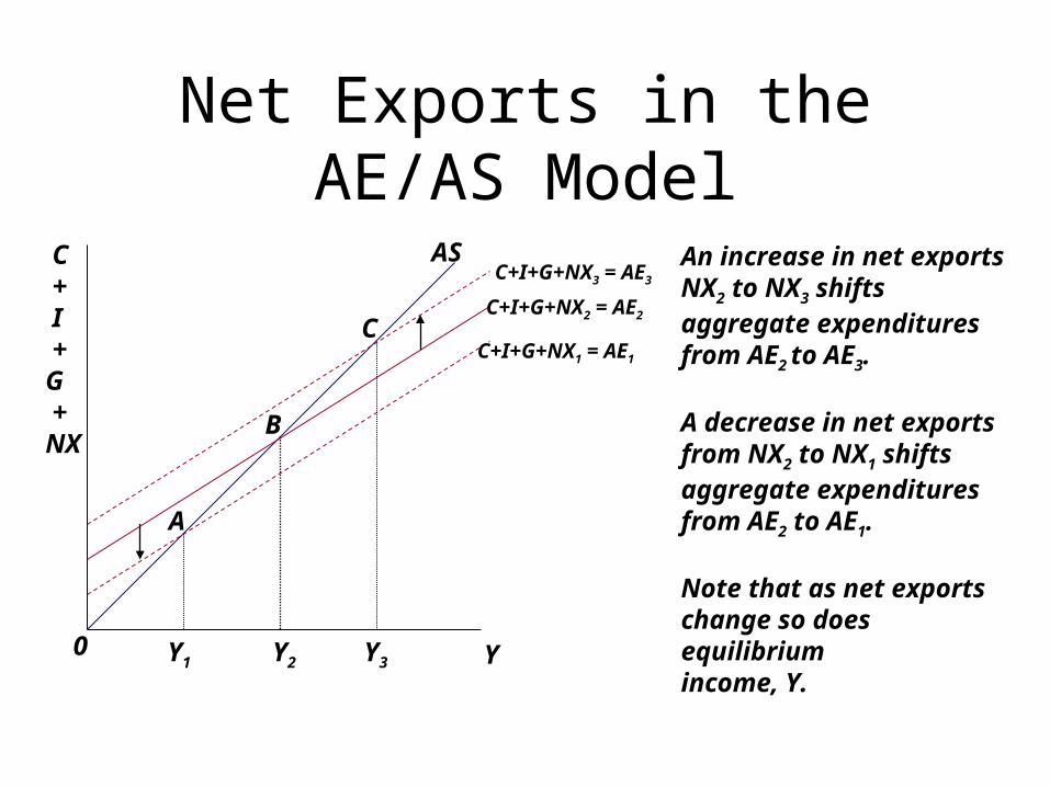
Net Exports in the AE/AS Model
C + I +G +NX
Y
AS
0
C+I+G+NX1 = AE1
C+I+G+NX3 = AE3
Y1 Y2 Y3
B
A
An increase in net exportsNX2 to NX3 shiftsaggregate expenditures from AE2 to AE3.
A decrease in net exportsfrom NX2 to NX1 shifts aggregate expenditures from AE2 to AE1.
Note that as net exportschange so does equilibrium income, Y.
C+I+G+NX2 = AE2
C

Practice
• How will the following events affect the aggregate expenditure line and national income? Why?– An increase in consumer optimism– A decrease in taxes paid by consumers– A rise in the general price level– A rising preference for BMWs– A rise in the stock market– An increase in government spending– Real wealth increases– Interest rates decline– A fall in the value of the dollar
Equilibrium in the Model
• When the model is in equilibrium, all goods and services produced are demanded by the members of the various sectors of the economy.– Aggregate expenditures = Aggregate supply
• The equilibrium in this model is stable.– There are forces built into the model that push it
towards equilibrium.
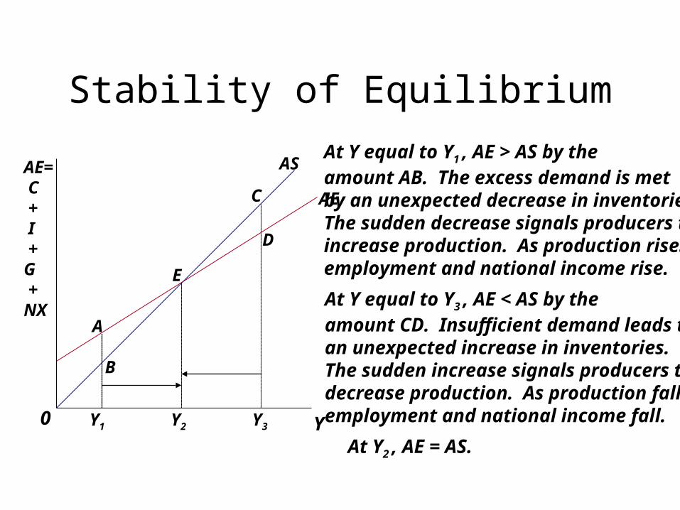
Stability of Equilibrium
AE= C + I +G +NX
Y
AS
0
B
A
C
Y1 Y2 Y3
E
D
AE
At Y equal to Y1 , AE > AS by the amount AB. The excess demand is metby an unexpected decrease in inventories.The sudden decrease signals producers toincrease production. As production rises,employment and national income rise.
At Y equal to Y3 , AE < AS by the amount CD. Insufficient demand leads toan unexpected increase in inventories.The sudden increase signals producers todecrease production. As production falls,employment and national income fall.
At Y2 , AE = AS.

Equilibrium with Algebra
Y = C + I + GC = a + bYd
Yd = Y - TI = IG = GY = a + b(Y-T) + I + GY = a + bY - bT + I + GY - bY = a - bT + I + GY(1 - b) = a - bT + I + GY = a - bT + I + G/(1-b)
Y = C + I + GC = 300 + 0.8Yd
Yd = Y - 1200I = 900G = 1300Y = 300 + 0.8(Y-1200) + 900 + 1300Y = 300 + 0.8Y - 960 + 900 + 1300Y = 1540 + 0.8YY - 0.8Y = 1540Y(1-0.8) = 1540Y = 1540/0.2 = 7700

Practice Y = C + I + G
C = 100 + 0.9 Yd
Yd = Y - T
T = 30, I = 250, G = 300• Find equilibrium Y.• Let the MPC = 0.8 and all other variables remain the
same and find equilibrium Y.• Let the MPC = 0.9 and taxes increase to 40 and find
equilibrium Y.• Is the equilibrium stable? Why?
The Multiplier
• The multiplier is the ratio of the change in equilibrium GDP (Y) divided by the original change in spending that causes the change in GDP.– Investment multiplier = /\Y//\I– Government spending multiplier = /\Y//\G
• GDP changes by a greater amount because a single change in spending ripples through the economy changing production, employment, and consumption again and again.

Multiplier Process
AE
Y
AS
0
B
Y1 Y2
E1
AE1
AE2
E2
The multiplier process begins at aninitial equilibrium level of Y such as Y1,where AE=AS.
It is initiated by an autonomous changein spending that causes AE to exceed AS. We show that change as a shift in AE fromAE1 to AE2. Now at Y1, AE is greater thanAS by the amount BE1.
At this point, inventories fall and are replaced with new production that causesan increase in employment. As employmentincreases, income increases, and as incomeincreases, consumption rises.
We are now at D. We repeat the processuntil we reach E2.
C
DF
G

Multiplier: Example
• Let /\I = 100 and the MPC = 0.8
• /\I /\Yd /\C /\S• 100 100 80 20
• 80 64 16
• 64 51.2 12.8
• 51.2 40.96 10.2
• 40.96 32.76 8.2
• 500 400 100

Multiplier Formulas• The numerical value of the multiplier can be found with
the following formulas:– The formula for the investment and government spending
multiplier is: • m = 1/(1-b) or equivalently m = 1/MPS
– The formula for the lump-sum tax multiplier is:• m = -b/(1-b) or equivalently m = -b/MPS
• Note that (1-b), the MPS, represents spending that is not occurring. – It is a leakage out of the spending stream, and as it becomes
larger, the multiplier becomes smaller.
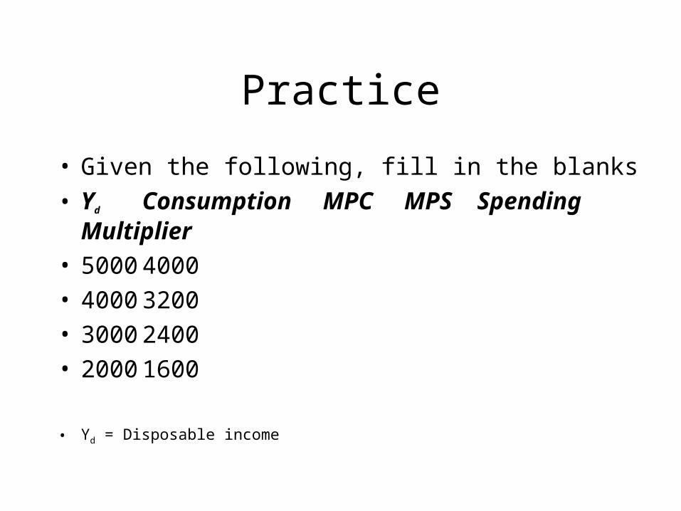
Practice
• Given the following, fill in the blanks
• Yd Consumption MPC MPS Spending Multiplier
• 5000 4000• 4000 3200• 3000 2400• 2000 1600
• Yd = Disposable income
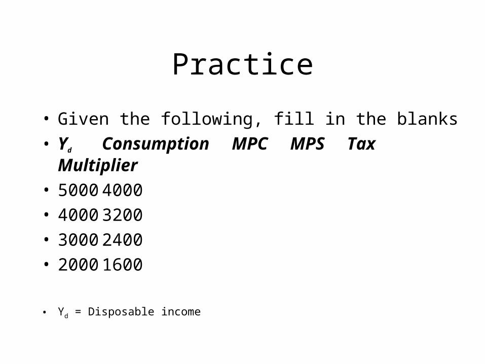
Practice
• Given the following, fill in the blanks
• Yd Consumption MPC MPS Tax Multiplier
• 5000 4000• 4000 3200• 3000 2400• 2000 1600
• Yd = Disposable income

Practice
• Fill in the blanks in the table below:
• MPC Multiplier Change in Y if /\I = $1000
• 0.9• 0.8• 0.75• 0.6• 0.5

Practice
• If the MPC is 0.9, and the government increases spending by 1.7 billion, by how much will Y change?
• If the MPC is 0.9, and the government increases taxes by 1.7 billion, by how much will Y change?
• If the MPC is 0.9, and the government simultaneously increases spending and increases taxes by 1.7 billion, by how much will Y change?
• Any thoughts?


