

THE OPTION TRADER’S GUIDE TO PROBABILITY, VOLATILITY, AND TIMING
TEAMFLY
Team-Fly®

Founded in 1807, John Wiley & Sons is the oldest independentpublishing company in the United States. With offices in NorthAmerica, Europe, Australia, and Asia, Wiley is globally commit-ted to developing and marketing print and electronic productsand services for our customers’ professional and personal knowl-edge and understanding.
The Wiley Trading Series features books by traders who havebeen able to work with the market’s ever changing temperamentand prosper—some by reinventing systems, others by gettingback to basics. For the novice trader, professional, or somewherein between, these books will provide the advice and strategiesneeded to prosper today and well into the future.
For a list of available titles, please visit our Web site at www.WileyFinance.com.

A Marketplace Book
THE OPTION TRADER’S GUIDE TO PROBABILITY,VOLATILITY, AND TIMING
Jay Kaeppel
John Wiley & Sons, Inc.

Copyright © 2002 by Jay Kaeppel. All rights reserved.
Published by John Wiley & Sons, Inc., New York.
Published simultaneously in Canada.
No part of this publication may be reproduced, stored in a retrieval system,or transmitted in any form or by any means, electronic, mechanical,photocopying, recording, scanning, or otherwise, except as permitted underSection 107 or 108 of the 1976 United States Copyright Act, without eitherthe prior written permission of the Publisher or authorization throughpayment of the appropriate per-copy fee to the Copyright Clearance Center,222 Rosewood Drive, Danvers, MA 01923, (978) 750-8400, fax (978) 750-4744.Requests to the Publisher for permission should be addressed to thePermissions Department, John Wiley & Sons, Inc., 605 Third Avenue, NewYork, NY 10158-0012, (212) 850-6011, fax (212) 850-6008, e-mail:[email protected].
This publication is designed to provide accurate and authoritativeinformation in regard to the subject matter covered. It is sold withthe understanding that the publisher is not engaged in rendering professionalservices. If professional advice or other expert assistance is required, theservices of a competent professional person should be sought.
Wiley also publishes its books in a variety of electronic formats. Somecontent that appears in print may not be available in electronic books. Formore information about Wiley products visit our Web site atwww.wiley.com.
ISBN: 0-471-22619-X
Printed in the United States of America.
10 9 8 7 6 5 4 3 2 1

In loving memory of Arthur H. Kaeppel


Contents
Chapter 1 Introduction 1
Who Can Benefit from This Book 1What Sets This Book Apart 2Can Options Really Be Simplified? 2What This Book Provides 2Overview of Option Trading 3Understanding Risk by Using Risk Curves 6Asking the Right Question 9Analyzing Risk: What Separates the Winners
from the Losers 11Summary 18
Chapter 2 The Basics of Options 21
Option Definitions 21Options on a Specific Security 26Intrinsic Value versus Extrinsic Value 30In-the-Money versus Out-of-the-
Money Options 32Summary 35
Chapter 3 Reasons to Trade Options 37
The Three Primary Uses of Options 37Leveraging an Opinion on Market Direction 39
vii

Hedging an Existing Position (and Generating Income) 41
Taking Advantage of Neutral Situations 44Summary 46
Chapter 4 Option Pricing 47
Theoretical Value 47Examples of Theoretical Option Pricing 49Overvalued Options versus Undervalued
Options 50Summary: Theory versus Reality 52
Chapter 5 Time Decay 55
The Effect of Time Decay on the Price of an Option 56
Implications of Time Decay 58Time Decay Illustrated 58Summary 62
Chapter 6 Volatility 63
Volatility: The Most Important Concept in Option Trading 63
Historic Volatility Explained 63Implied Volatility Explained 65Is Implied Volatility High or Low? Relative
Volatility Explained 69Relative Volatility Ranking 72Considerations in Selecting Option-
Trading Strategies 72Why Does Volatility Matter? 74The Effect of Changes in Volatility 77Summary 80
viii Contents

Chapter 7 Probability 81
Weighing the Pros and Cons 81Strategies for a Bullish Scenario 82Profit/Loss Comparisons 86Delta 89Probability Analysis 91The Correct and Incorrect Ways to
Use Probability 95Summary 96
Chapter 8 Market Timing 99
The Underlying Security Is Expected to Move within a Specific Period 100
The Underlying Is Expected to Move in a Particular Direction but Not in a Specific Time Frame 102
The Underlying Is Expected to Move Significantly but the Direction Is Unknown 103
The Underlying Is Expected to Stay within a Range or Not Move Much in Any Direction 105
Summary 106
Chapter 9 Trading Realities 107
Exercise and Assignment 107Bid and Ask Prices and the Importance of
Option Volume 110Appreciating the Effect of Bid-Ask Spreads 111Factors in Dealing with Bid-Ask Spreads 113A Word on Limit Orders 113Summary 115
Chapter 10 Important Concepts to Remember 117
Valid Reasons to Trade Options 117Option Pricing 118
Contents ix

Time Decay 118Volatility 119Probability 120Market Timing 120How to Lose Money Trading Options 121The Keys to Success in Option Trading 125Summary 128
Chapter 11 Overview of Trading Strategy Guides 131
The Two Key Elements in Selecting a Trading Strategy 131
Trading Strategy Matrix 133Overview of Trading Strategy Chapters 133
Chapter 12 Buy a Naked Option 139
Key Factors 139Position Taken 146Position Management 148Trade Result 150
Chapter 13 Buy a Backspread 151
Key Factors 151Position Taken 157Backspreads versus Naked Calls and Puts 157Volatility and Backspreads 159Position Management 162Trade Result 164
Chapter 14 Buy a Calendar Spread 165
Key Factors 165Position Taken 173Position Management 173Trade Result 174
x Contents
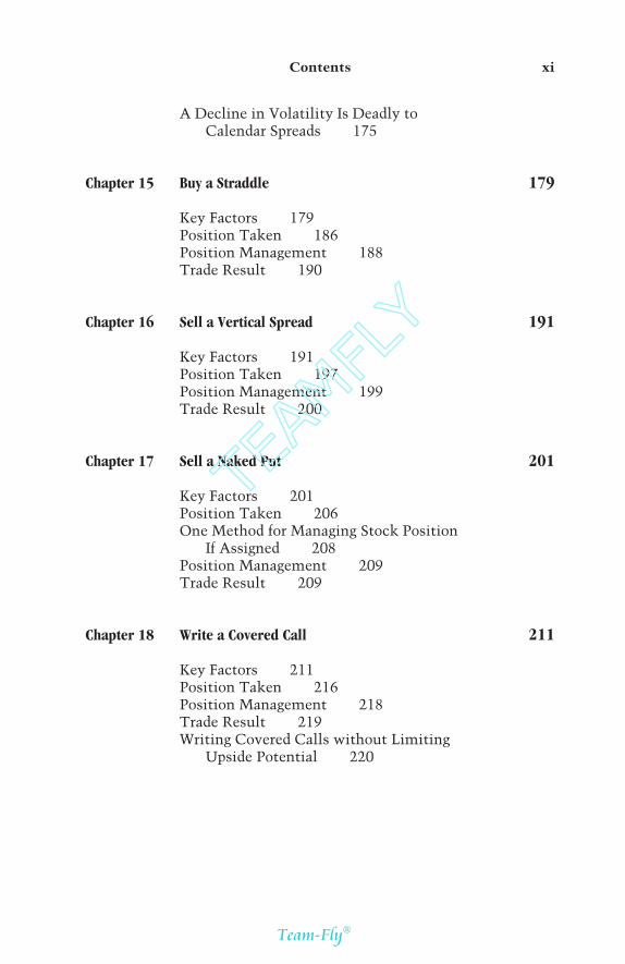
A Decline in Volatility Is Deadly to Calendar Spreads 175
Chapter 15 Buy a Straddle 179
Key Factors 179Position Taken 186Position Management 188Trade Result 190
Chapter 16 Sell a Vertical Spread 191
Key Factors 191Position Taken 197Position Management 199Trade Result 200
Chapter 17 Sell a Naked Put 201
Key Factors 201Position Taken 206One Method for Managing Stock Position
If Assigned 208Position Management 209Trade Result 209
Chapter 18 Write a Covered Call 211
Key Factors 211Position Taken 216Position Management 218Trade Result 219Writing Covered Calls without Limiting
Upside Potential 220
Contents xi
TEAMFLY
Team-Fly®
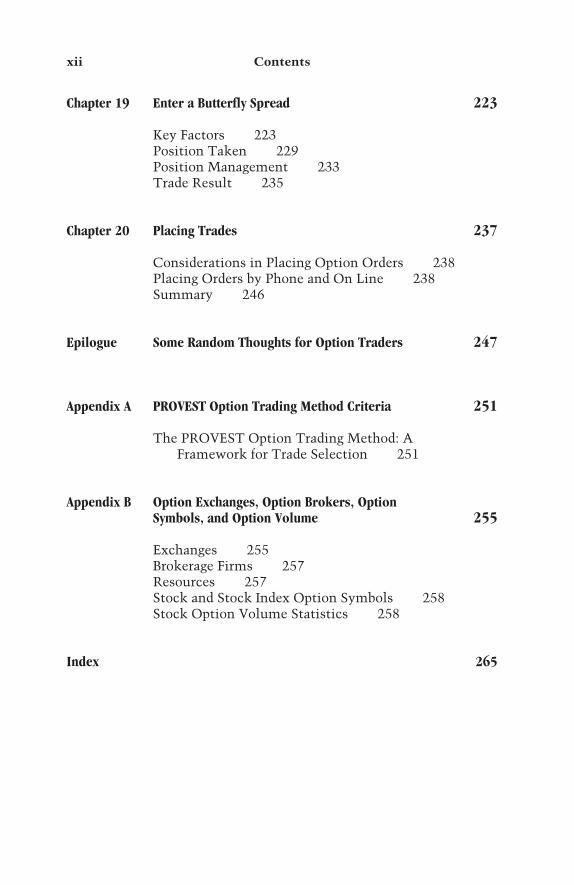
Chapter 19 Enter a Butterfly Spread 223
Key Factors 223Position Taken 229Position Management 233Trade Result 235
Chapter 20 Placing Trades 237
Considerations in Placing Option Orders 238Placing Orders by Phone and On Line 238Summary 246
Epilogue Some Random Thoughts for Option Traders 247
Appendix A PROVEST Option Trading Method Criteria 251
The PROVEST Option Trading Method: A Framework for Trade Selection 251
Appendix B Option Exchanges, Option Brokers, Option Symbols, and Option Volume 255
Exchanges 255Brokerage Firms 257Resources 257Stock and Stock Index Option Symbols 258Stock Option Volume Statistics 258
Index 265
xii Contents

xiii
Foreword
Novice traders are attracted to the options market because of thedegree of leverage and the vision of enhanced profitability it af-fords them. Options, however, are unlike any other exchange-traded product because of leverage, and more importantly,because of an attribute referred to as time decay. Unfortunately,traders learn the hard way that many factors besides calling themarket direction correctly come into play in trading options.Most traders do not understand implied volatility, time decay,and out-of-the-money versus in-the-money options. Many do nothave a working knowledge of which option strategies are best forany given situation, and they fail to understand just what therisk is before they make their trades.
Jay Kaeppel explains these issues in The Option Trader’sGuide to Probability, Volatility, and Timing. Kaeppel covers thebasics and then goes on to teach how to trade options. Andhe doesn’t do it with get-rich-quick examples and hyperbole. Helooks at the options market with a thorough analysis of boththe risk and the profit potential of the various strategies, and hedoes so in a very readable fashion.
Kaeppel outlines the steps involved in becoming a successfultrader. He explains the different strategies available and when touse each one. He shows how to accurately assess volatility andfrom there, how to profit by disparities in the implied volatilitiesof different options. His strategies include guidelines for deter-mining when to buy undervalued options and when to sell over-valued options. Finally, Kaeppel teaches when to take a profit,and most importantly, when to cut losses and move on to thenext trade.
The key value of this book is its objectivity and its details.The guidelines are clear and objective, not a collection of anec-dotal examples that have happened once or twice. Save yourselfsome money and benefit from this money manager’s experienceand wisdom if you want to profit in the options market.
THOM HARTLE
2001
Thom Hartle (www.thomhartle.com) is a trader and educatorworking with private trades, as well as a contributing editor forActive Trader Magazine.
xiv Foreword

Chapter 1
INTRODUCTION
1
Who Can Benefit from This Book
This book is written for people who fall into one of twocategories:
1. Those who are new to option trading and looking for a goodplace to start
2. Those who have traded options in the past and did notachieve the type of success they had hoped to
Option trading enjoyed explosive growth during the late1990s and into the start of the new millennium, particularlyamong individuals. Traders whose bankrolls were fattened bythe great bull market in stocks fueled part of this growth. Havingenjoyed great success in the stock market, many people decidedto try to increase their gains by accessing the leverage associatedwith options. Along the way computers got faster and morepowerful, technology advanced rapidly, and markets traded withgreater volume and volatility than ever before. Yet there is muchabout option trading that is no different than it ever was.Through all the years and all the growth and changes, critical el-ements remain that traders must understand and apply consis-tently if they hope to succeed in the long run. The purpose ofthis book is to illuminate these concepts and show how to applythem successfully in real-world trading.

What Sets This Book Apart
The primary focus of this book is not to teach you about options,but rather to teach you how to successfully trade options. Havinga textbook understanding of any topic is not the same thing as ap-plying that knowledge in the real world. This book is intended togive new traders and returnees to the options market an under-standing of what it takes to succeed, as well as a set of guidelinesto apply in the real world of trading. Most of all, it is intended tomake traders aware of the sobering realities of option trading, in-cluding the financial risks involved. No attempt is made tocandy-coat the fact that garnering consistent profits in the op-tions market over a long period is a difficult goal to achieve.
Can Options Really Be Simplified?
Options are by nature fairly complex. Not only are there manytrading strategies to consider, there also are many different fac-tors that apply to trade selection and position management. Tocomplicate things even further, some factors matter a lot withcertain strategies and not as much with others. Nevertheless,despite the inherent complexities, it is possible to gain an un-derstanding of these key factors without a Ph.D. in finance. Thisbook will introduce you to the most important basic conceptsin option trading and illustrate why an understanding of theseconcepts is critical to your long-term success. In the later chap-ters of this book, the concepts are applied to a number of differ-ent trading strategies to show you how to get the most out ofeach situation.
What This Book Provides
A careful reading of the material in this book will give you thefollowing:
• An introduction to the most valuable uses of options• Basic option terminology
2 The Option Trader’s Guide

• Explanations of the most important concepts in optiontrading
• Explanations of the most useful trading strategies available• The conditions to look for when deciding which strategy to
employ• Objective guidelines for employing each strategy• Objective guidelines for exiting a trade at a loss• Objective guidelines for exiting a trade at a profit
Overview of Option Trading
Most option traders use options simply as a tool to leverage theirmarket-timing decisions. They buy call options when they thinkan advance is imminent and they buy put options when theythink a decline is forthcoming. Unfortunately, because buyingcalls and puts involves buying a wasting asset, in most casesthis approach ends up being unprofitable. It is estimated that90% or more of people who trade options lose money in the longrun. If this is true, it is a staggering number. However, a highfailure rate is not all that surprising when you consider the com-plexity involved in trading options and the fact that most optiontraders do not take the time to develop a well-thought-out planbefore they begin trading. In addition, many traders are poorlyprepared to deal with the emotional aspects of trading.
It is vitally important to your long-term success that youuse a structured approach to trading.
This is not to imply that your trading approach must be com-pletely systematic. What it means is that you must establish andfollow some reasonably well-thought-out guidelines if you hopeto achieve consistent success. Markets can turn on a dime. If youdo not have a well-thought-out trading plan, you will find your-self chasing each twist and turn of the market. In addition, if youdo not develop the discipline to follow your trading plan, theodds are overwhelming that you will join the 90% of traders wholose money.
Introduction 3

To go one step further, not only should you have a plan be-fore you start trading, you must plan each option trade in termsof how you will manage each position once you have enteredinto it. There is no one best trading strategy; each one hasstrengths and weaknesses. By examining the best-case andworst-case scenarios for each trade, you can establish objectivecriteria for when to exit each trade, whether you are taking aprofit or cutting a loss.
Too many traders enter the markets on a whim, withoutcarefully considering either
• The likelihood that they will be successful in the long run• The potential pitfalls they may encounter and what they can
do to avoid them
The material in this book is written to help you as a trader byproviding a specific trading plan, using well-thought-out andmarket-tested criteria for entering and exiting each trade. It isalso intended to help you hone your ability to think like a traderby walking you through example trades to let you develop a feelfor the process of deciding on
• Strategy selection• Individual trade selection• Position-management guidelines
Each strategy chapter in this book (Chapters 12 through 19)delineates a specific set of rules for each strategy. Be assured thatthere is no intent to convince you that this is the only way to usea given strategy. The underlying point is my belief that tradersare better off in the long run if they adopt one approach they arecomfortable with for a given strategy than if they make it up asthey go along, using one approach one time and a different ap-proach the next time.
The Benefits of an Objective Approach
Traders gain a psychological benefit from doing their best thinkingup front and building a well-thought-out trading plan. After that,
4 The Option Trader’s Guide

they are simply following the rules. One thing to remember isthat your trading plan will not always maximize your profit oneach and every trade. This is simply a reality of trading. The bene-fits of using an objective approach to option trading include these:
• Eliminating emotional decision making• Relieving the psychological burden of being right or wrong in
each situation• Doing your best thinking up front and then trusting in your
plan, rather than having to make subjective decisions in theheat of battle
Constructing a well-thought-out trading plan is a crucial steptoward consistent trading success. A trading plan relieves a greatdeal of the emotional pressure that traders feel when they rely ongut instinct and hunches to trade. Too many traders assume thatthey will know the right thing to do when the time arrives. In re-ality, more often than not this turns out to be exactly the oppo-site of what actually occurs. In a bad situation, with real moneyon the line, unprepared traders make emotional decisions basedsolely on fear or greed. Very often these are decisions that theywould never make if they were thinking rationally.
The good news about developing a trading plan is that a well-thought-out plan can serve as a road map to trading profits bykeeping you from overreacting to every bend in the road. The badnews is that no approach to trading is perfect. There are no magicformulas or holy grail for trading.
The surest way to succeed as a trader is to develop a trad-ing approach that has a realistic probability of makingmoney in the long run and then to stick to your plan.
Here are the key steps in this process.
1. Identify criteria that give you the greatest probability of suc-cess in the long run.
2. Develop confidence in the approach you are using. Confi-dence comes from establishing criteria that cover all the fol-lowing bases:
Introduction 5

• When to use a particular strategy• When to enter a trade• When to exit a trade at a profit• When to exit a trade at a loss
3. Develop the discipline to stick to your approach even whenthings are not going well. This comes from having the confi-dence developed in Step 2.
Once you reach this point, your trading process becomes secondnature. Through good times and bad you continue to trade con-sistently, confident that in the long run you will come out ahead.This is a trait of all successful traders.
Understanding Risk by Using Risk Curves
A risk curve is a graph that depicts the profit or loss characteris-tics for a given option trade. Analyzing a risk curve allows atrader to visualize the market action needed to make money onthat particular trade. Such a graph is also useful in assessing
• Break-even points and probability of profit• Maximum risk• Profit potential
Additionally, two or more risk curves can be analyzed to deter-mine which trade offers the reward-to-risk characteristics atrader deems most attractive.
More than anything, a risk curve is a forest-from-the-treestool. For any option trade, it does not really matter in the endwhat the position is—whether it is long a call, long a spread,short a spread, or any other combination. In the final analysis theonly questions that matter are these:
• What has to happen in order for me to make money on thistrade?
• What is my worst-case scenario?
A risk curve allows you to visualize the answer to these all-important questions. Risk curves are used throughout this book
6 The Option Trader’s Guide

to depict the profit and loss characteristics of various trades. Let’slook at an example to help you understand what these graphsshow and why the information they contain is so important.
Figure 1.1 shows risk curves for a position that involves buy-ing the IBM February 85 call option on January 5 at a price of13.25 ($1325). A range of prices for the stock is listed along thebottom of the graph, with the current price of 94 in the middle.The graph shows the profitability of this trade based on an un-derlying stock price ranging from 79 to 104. The actual expecteddollar profit or loss is listed on the left side of the graph.
Each curve on the graph displays the expected profit or loss ata given stock price as of a given date. This trade was initiated onJanuary 5. The top curve shows the expected return as of January12, the next curve as of January 19, then January 26, February 2,February 9, and finally, the date of the February option expira-tion, which is February 16. Much useful information may begleaned from this graph.
The Effect of Time Decay
The first thing to note is the effect of time decay. As we discussin detail in Chapter 5, time decay refers to the erosion of an
Introduction 7
Date: 2/16/01 Profit/Loss: –10 Underlying: 98.22 Above: 39% Below: 61% % Move Required: +4.2%
1325
883
442
0
–442
–883
–132579.00 84.00 89.00 94.00 99.00 104.00 109.00
Figure 1.1 Risk curves for IBM February 85 call option (from 79 to 109).
TEAMFLY
Team-Fly®

option price as time passes and option expiration draws nearer.The obvious implication from this graph is that the buyer of thisoption stands to earn a greater profit if the price of the stockrises sooner rather than later. As the price of the option erodesslightly with each passing day due to time decay, a larger pricemove by the underlying security is required to offset this loss.
Break-Even Analysis and Probability of Profit
The lowest curve on the graph in Figure 1.1 displays the ex-pected profit or loss if the option is held until expiration. Al-though many options are exited before expiration, it is oftenhelpful to know where a trade is going to end up eventually if thetrader does nothing before expiration. In this case the break-evenpoint is 98.25 (which equals the strike price of 85 plus the pricepaid for the option of 13.25). Based on the volatility of IBM stockwhen this trade is entered, there is a 39% probability that IBMwill rise from 94 to 98.25 or higher by the time of February op-tion expiration. This probability value is most useful when com-pared to the probability value for another potential trade. Bycomparing two or more trades, a trader can determine which ismost likely to generate a profit.
Maximum Risk
Whenever you buy an option, your risk is limited to whateverprice you paid to buy the option. In this example the buyer paid$1325 to buy the option. You can see by the lowest curve on thegraph in Figure 1.1 that the maximum loss will occur if the stockis trading at 80 or lower at the time of option expiration. In otherwords, even if IBM stock fell to 70 or 60 or 50 or less, the optionbuyer’s loss in this example would never exceed $1325. This il-lustrates the limited risk feature associated with buying options.
Profit Potential
In addition to limited risk, buying an option gives a trader un-limited profit potential. Figure 1.2 shows the same trade as that
8 The Option Trader’s Guide

in Fugure 1.1. The only difference is that the price range alongthe bottom of the graph has been expanded from 15 points aboveand below the current price of the stock to 40 points above andbelow the current price of the stock. This range is expanded to il-lustrate the profit potential available if IBM makes a substantialmove in price.
As you can see, if IBM were to rally 40 points by option ex-piration, the buyer of this option could earn a profit of $3620 ona $1325 investment. Although the probability of this happeningmay be low, it represents a return of 173% and vividly illustratesthe huge profit potential of buying options.
Asking the Right Question
Too many traders focus on probability or profit potential andcompletely ignore risk.
When assessing the prospects for any given trade, the rightquestion is not “How much can I make?” The right question is“What is my worst-case scenario and how do I mitigate thisrisk?” According to an old adage in trade, “As long as you mini-mize losses, profits will take care of themselves.”
Introduction 9
Date: 2/16/01 Profit/Loss: 10 Underlying: 98.33 Above: 39% Below: 61% % Move Required: +4.3%
3620
2715
1810
905
0
–905
–181154.00 67.31 80.69 94.00 107.31 120.69 134.00
Figure 1.2 Risk curves for IBM February 85 call option (from 54 to 134).

Most traders new to options are attracted by the lure of easymoney. This is not all that surprising. Most advertisements foroption trading play on traders’ desire to make a lot of money fast.Traders read ads claiming that they can double or triple theirmoney in a matter of a few short weeks, pinpoint tops and bot-toms, or trade without risk. It is not as though all traders are sonaïve as to completely buy into this type of hype, but over timethere can be a cumulative effect. Eventually a trader thinks,“Well, if so many people claim it is possible, there must be sometruth to it.” Thus, many new option traders enter the tradingarena with stars in their eyes. Unfortunately, these are thetraders who are most likely to experience the jarring jolt of real-ity when they actually start entering positions and find out thereal secret of trading.
The real secret of trading is simply that there is no easymoney to be made in trading!
Bad things happen even to the very best traders:
• Markets often reverse unexpectedly or gap sharply in thewrong direction.
• Markets can be choppy and trendless for frustratingly longperiods.
• Buy orders get filled at the high of the day.• Sell orders get filled at the low of the day.• If you increase your trading size after a string of winners, the
next trade will be a big loser.• If you stop trading after a string of losers, the next trade you
don’t take will be a big winner.
It is how one reacts to unpleasant experiences that sepa-rates the long-term winners from the 90% of traders wholose money.
One of the keys to trading success is to avoid the big hit. Onedevastating loss can wipe out a significant portion of your trad-
10 The Option Trader’s Guide

ing capital, and the psychological damage can be irreparable,often rendering a trader incapable of functioning rationally on fu-ture trades. You are much more likely to be successful if you rec-ognize, acknowledge, and plan out how you will deal with theworst-case scenario in each instance than you are if you believeblindly that whatever it is you are doing will somehow prevail,even in the face of extremely adverse conditions.
If you look at each trade you make and identify the worst-case scenario that might result, you can develop an objectiveplan in advance for dealing with that possibility. This allowsyou to build a safety net, which can keep you from suffering thedevastating big hit.
Before you worry about making big money, you must in-sulate yourself from the danger of losing big money. Theonly way to do this is to address risk before reward.
Analyzing Risk: What Separates the Winners from the Losers
One key to making money is to avoid losing money!To avoid losing money you must
• Acknowledge the downside risk of any trade• Develop a contingency plan to deal with this risk
The one thing you cannot do is pretend that risk doesn’texist!
If you asked traders who have enjoyed long-term success forthe key to their success, the vast majority of them would tell youit was
• Cutting losses• Controlling risk
Everybody gets into trading to make money. It is interestingthat those who end up being most successful in this endeavor
Introduction 11

often spend more time focusing on not losing money than theydo on making money.
One of the keys to option trading success is understand-ing the risks involved in any trade and then planning tominimize these risks.
When traders learn about option-trading strategies, theyoften don’t receive enough information to fully understand therisks involved. In the following pages are two case studies oftrades that, on the surface, could be touted by market gurus ashigh-probability, sure-thing, you-can’t-lose trades. In fact, mostdiscussions of these strategies fail to answer the right question—“What is my risk on this trade?”
Novice traders are quick to latch onto ideas that promise thepotential for huge profits. Unfortunately, too many traders aresubconsciously content as long as they believe they have a chanceto make a lot of money, regardless of the reality of the situation.Whether the trades actually work out or not ends up being a sec-ondary consideration. Until the mounting losses become toogreat, they continue to hope that the next trade will be the big one.
Too often, traders are so focused on the idea of making alot of money that they fail to account for or even ac-knowledge the risks involved in the trades they make.This is the road to trading failure.
Case 1: Ratio Spread
The trade presented in Figure 1.3 looks extremely enticing.The strategy used in this trade is referred to as a ratio spread.This trade uses options on Coffee futures and involves buyingone call option with a strike price of 700 and simultaneouslyselling two further-out-of-the-money options with a strike priceof 750. The risk curve shows the profit or loss that a trader hold-ing this position would experience if the trade were held until
12 The Option Trader’s Guide

option expiration. The expected dollar profit or loss is listeddown the left side of the graph, and a range of underlying pricesare listed across the bottom of the graph.
If the trade is held until option expiration, there is
• A 91% probability of profit. In other words, with Coffee trad-ing at 6765 when the trade is entered, there is a 91% proba-bility that Coffee will be trading below the break-even priceof 8098 at the time of option expiration.
• Unlimited risk if Coffee is above 8098. However, when thetrade is entered, there is only a 9% probability of Coffeerising from 6765 to 8098 or higher by the time of optionexpiration.
• A maximum profit potential of $2032.• A guaranteed profit if Coffee stays at 7000 or below.
This trade inarguably offers some great potential benefits.However, looking at this trade only at expiration fails to answerthe most important questions. The most important questions toanswer before entering any trade are not “How much can Imake?” or “What is the probability that I will profit?” The ques-tions you need to answer are “How bad can things get?” and“What do I plan to do about it?”
Introduction 13
2092
558
–976
–25114765 5432 6098 6765 7432 8098 8765
Date: 5/07/01 Profit/Loss: –6 Underlying: 8098 Above: 9% Below: 91% % Move Required: +19.9%
Figure 1.3 Risk curve for Coffee call ratio spread at expiration.
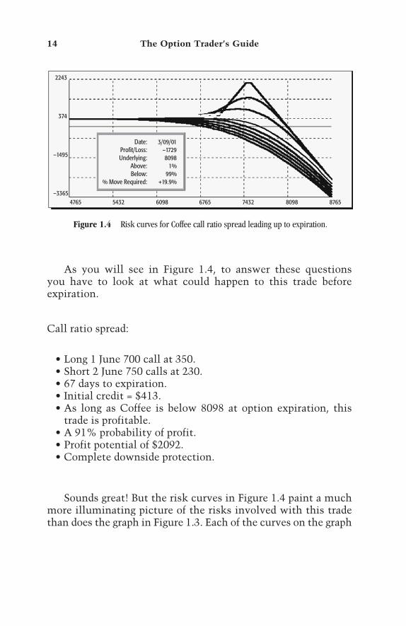
As you will see in Figure 1.4, to answer these questionsyou have to look at what could happen to this trade beforeexpiration.
Call ratio spread:
• Long 1 June 700 call at 350.• Short 2 June 750 calls at 230.• 67 days to expiration.• Initial credit = $413.• As long as Coffee is below 8098 at option expiration, this
trade is profitable.• A 91% probability of profit.• Profit potential of $2092.• Complete downside protection.
Sounds great! But the risk curves in Figure 1.4 paint a muchmore illuminating picture of the risks involved with this tradethan does the graph in Figure 1.3. Each of the curves on the graph
14 The Option Trader’s Guide
2243
374
–1495
–33654765 5432 6098 6765 7432 8098 8765
Date: 3/09/01 Profit/Loss: –1729 Underlying: 8098 Above: 1% Below: 99% % Move Required: +19.9%
Figure 1.4 Risk curves for Coffee call ratio spread leading up to expiration.

depict the expected profit or loss as of a different date based onthe price of Coffee at that time. A range of Coffee prices is listedalong the bottom of the graph.
By looking at the risk curves on several dates leading up toexpiration, we get a more realistic picture of the risk involved.The real risk in this trade is not that Coffee will be trading above8098 at the time of option expiration. The real risk in this tradeis that Coffee prices will experience a sustained move upwardimmediately after the trade is entered. If Coffee rallies soonerrather than later, traders may be holding a trade with a largeopen loss. Although the probability of this happening may below, when you consider that Coffee once opened 3000 pointshigher, you can begin to appreciate the need to acknowledge thatsuch a thing could happen and the potential impact that such amove could have on this trade. Therefore, you need to know howsuch a move would affect your position to ensure that you couldweather the worst-case scenario.
The key is not in figuring out what to do once the worst-case scenario unfolds. The key is advance planning toavoid getting into such a situation in the first place.
This type of planning would be impossible if you looked onlyat the risk curve at expiration, which is what the graph in Figure1.3 shows. Unfortunately, the graph showing how the tradewould work out if it were held until expiration is the one thatusually shows up when option-trading strategies are discussed.As you can see in Figure 1.4, the single risk curve drawn at expi-ration does not tell the full story.
It is impossible to overemphasize the importance of recog-nizing the risks that exist for any given trade and planning in ad-vance to minimize risk should the worst-case scenario unfold,rather than waiting for the worst to happen and then trying tofigure out how to save your skin!
There is a 91% probability of profit if the position is held toexpiration; however,
Introduction 15

• If Coffee rallies sharply before expiration, large unlimitedlosses can occur!
• Maximum profit potential of $2092 occurs only if Coffeecloses exactly at 7500 at expiration!
Case 2: Synthetic Long Futures Position
The trade presented in Figure 1.5 appears to be close to a surething. The strategy used in this example is referred to as a syn-thetic long futures position. The trade is established by buyingan out-of-the-money call and simultaneously writing an out-of-the-money put. The risk curve depicts the profit or loss for atrader holding this position if the trade is held until option expi-ration. The expected dollar profit or loss is listed down the leftside of the graph, and a range of underlying futures prices arelisted across the bottom of the graph.
If this trade is held until expiration,
• There is an 80% probability of profit. In other words, withS&P 500 futures trading at 1239 as the trade is entered, thereis an 80% probability that S&P 500 futures will be tradingabove the break-even price of 1170 at the time of option ex-piration.
16 The Option Trader’s Guide
6146
1639
–2868
–7375113950 117283 120616 123949 127283 130616 133949
Date: 4/19/01 Profit/Loss: –16 Underlying: 117003 Above: 80% Below: 20% % Move Required: –5.7%
Figure 1.5 Risk curve for S&P synthetic futures at expiration.

• There is unlimited risk if the S&P 500 falls below 1170.However, when this trade is entered there is only a 20%probability of the S&P 500 declining from 1239 to 1170 orlower by the time of option expiration.
• This trade has unlimited upside potential.
Unfortunately, just as in Case 1, looking at this trade only atexpiration fails to answer the most important question aboutrisk. Remember, the questions you need to answer are “Howbad can things get?” and “What do I plan to do about it?” To an-swer these questions, you must again look at what could happento this trade before expiration (see Figure 1.6).
Synthetic futures: long a call, short a put
• Long 1 Apr 1320 call at 1730.• Short 1 Apr 1175 put at 1830.• As long as S&P is above 1170 at option expiration, this trade
is profitable.• An 80% probability of profit.• Unlimited profit potential.
Sounds like a sure thing! But as with the Coffee trade inCase 1, the risk curves in Figure 1.6 paint a much more illumi-
Introduction 17
13760
4587
–4587
–13761113950 117283 120616 123949 127283 130616 133949
Date: 3/16/01 Profit/Loss: –7631 Underlying: 117004 Above: 94% Below: 6% % Move Required: –5.7%
Figure 1.6 Risk curves for S&P synthetic futures leading up to expiration.
TEAMFLY
Team-Fly®

nating picture of the risks involved with this trade than does thegraph in Figure 1.5. By looking at the risk curves on several datesbefore expiration, we get a more realistic picture of the riskinvolved.
The real risk in this trade is not that the S&P will fall below1170 at expiration. The real risk is that the S&P will declinesharply before expiration. If the S&P falls sooner than later, thetrader may be holding a large open loss. The key is not figuringout what to do once this occurs; the key is to plan in order toavoid getting into such a situation in the first place. This type ofplanning would be impossible if you looked only at the riskcurve at expiration, which was shown in the graph in Figure 1.5.Unfortunately, the graph showing how the trade would work outif it were held until expiration is the one that usually shows upwhen various option-trading strategies are discussed. As you cansee in Figure 1.6, the single profit/loss line drawn at expirationdoes not tell the full story.
NOTE
The purpose of this example is not to imply that synthetic futures are a badidea nor that option educational materials are purposefully misleading whenall they include is a profit/loss graph as of option expiration. The purpose issimply to illustrate the importance of identifying and planning for the risks in-volved with any trade. It is impossible to state definitively that this is a goodtrade or a bad trade—that is up to each trader to determine.
As long as the S&P is above 1170 at option expiration, thistrade is profitable; however, if S&P falls sooner than later, un-limited losses can occur!
Summary
The primary message to take away from this chapter is simplythat options differ in many ways from other forms of invest-ment. When you buy a stock or a futures contract, you eithermake a point for each point it rises in price, or you lose a point
18 The Option Trader’s Guide

for each point it declines. With options it is not always sostraightforward.
You should also prepare yourself to focus on the key ele-ments that must be understood and applied to achieve success inoption trading.
Introduction 19


Chapter 2
THE BASICS OF OPTIONS
21
Before one can hope to succeed in any field of endeavor, onemust have a firm grasp of the fundamental concepts. It is no dif-ferent in the field of option trading. Anyone can get lucky on atrade now and then, but a solid understanding of the basics is re-quired to achieve consistent long-term success. Option tradinghas a vocabulary all its own. In this chapter you will learn manycommon and essential terms.
When you buy or sell short a stock or a futures contract, theresults you can expect are fairly straightforward. If you buy 100shares of stock and that stock goes up 5 points, you will make$500. If it goes down 5 points, you will lose $500. With options,these simple parameters do not apply. Depending on the optionor options you choose to buy or write, your expected return andthe amount of risk you are exposed to can vary greatly. Beforedelving into these possibilities, let’s define some importantoption terms.
Option Definitions
Call option. A call buyer pays a premium to the optionwriter, which gives the option buyer the right, within aspecified period, to buy 100 shares of stock (or one fu-tures contract) at a specified price (known as the strikeprice), no matter how high the stock price may rise. Forexample, say a trader buys a call option with a strike price

of 50. The stock then rises to 100. By virtue of holding acall option with a strike price of 50, the trader can exer-cise the option and buy 100 shares of stock at a price of 50a share.
Put option. A put buyer pays a premium to the optionwriter, which gives the option buyer the right, within aspecified period, to sell 100 shares of stock (or one futurescontract) at a specific price, no matter how low the stockprice may fall. For example, say a trader buys a put optionwith a strike price of 50. The stock then falls to 10. Be-cause the trader holds a put option with a strike price of50, the trader can exercise the option and sell 100 sharesof stock at 50.
Underlying. In the world of options, the word underlyingrefers to the security on which a given option is based.For example, IBM is the underlying security for all IBMoptions. In futures markets, Soybean futures are the un-derlying for all Soybean options.
Option buyer. The person who buys an option.Option writer. The person who writes an option.Option premium. The price of an option contract. Stock
options are for 100 shares, so a stock option that is quotedat a price of $5 (or 5), represents an option premium of$500 (100 × $5). The option premium is the amount thatthe option buyer pays to the option writer. It also repre-sents the total amount of risk assumed by the buyer ofthe option and the maximum amount of profit that canbe obtained by the writer of the option.
Strike price or exercise price. The strike price is the price atwhich an option can be exercised, that is, the price pershare that the buyer of a call option must pay to buy thestock if the buyer chooses to exercise his or her option.Option exchanges designate the available strike prices foreach listed security. For most stocks the default range be-tween strike prices is 5 points (e.g., 25, 30, 35, 40). Manystocks also offer strike prices at 2.5-point incrementsbelow 30 (e.g., 2.5, 7.5, 12.5, 17.5, 22.5, 27.5). If a stock orstock index reaches a price above 200, the options oftentrade only in increments of 10 points or more (e.g., 250,
22 The Option Trader’s Guide

260, 270, 280). Strike prices for options on futures areset by the exchange and vary from commodity tocommodity.
Expiration date. The date after which an option is void andceases to exist is its expiration date. For U.S. stock op-tions, the expiration date is the third Friday of the expi-ration month. In other words, June options expire on thethird Friday in June, July options expire on the third Fri-day in July, and so on. For futures options, the expirationmonths and expiration dates can vary and are set by theexchange on which a given series of options is traded.
Expiration cycle. For U.S. stock options, the exchange onwhich the options are traded designates a particular expi-ration cycle—either a January cycle, February cycle,March cycle, or all months. The expiration months forthe options on a given stock are determined by the expi-ration cycle assigned to that stock.
Theoretical price or fair value. The price at which a givenoption is considered fairly valued based on a combinationof variables used in a standard option pricing model iscalled the option’s fair value (see Chapter 4 for more de-tails on option pricing).
In-the-money option. A call option is in the money if itsstrike price is less than the current market price of theunderlying. A put option is in the money if its strike priceis higher than the current market price of the underlying.
A call option with a strike price of 50 is considered inthe money as long as the price of the stock is greater than50. A put option with a strike price of 50 is considered inthe money as long as the price of the stock is less than 50.
Out-of-the-money option. An option that currently has nointrinsic value is an out-of-the-money option. A call op-tion is out of the money if its exercise price is higher thanthe current market price of the underlying. A put optionis out of the-money if its exercise price is lower than thecurrent price of the underlying.
A call option with a strike price of 50 is considered outof the money as long as the price of the stock is less than50. A put option with a strike price of 50 is considered out
The Basics of Options 23

of the money as long as the price of the stock is greaterthan 50.
At-the-money option. For any security, the option whosestrike price is currently closest to the actual price of theunderlying security is generally referred to as the at-the-money strike. Please note that, technically speaking,the at-the-money option is usually slightly in or out of themoney. For example, if a stock is trading at a price of 96,the 95 call and the 95 put options are considered the at-the-money strikes, even though the call option is 1 pointin the money and the put is 1 point out of the money.
Intrinsic value. The amount by which an option is in themoney is its intrinsic value. An out-of-the-money optionhas no intrinsic value. If a call option has a strike price of50 and the underlying stock is trading at 55, the 50 calloption has 5 points of intrinsic value. If a put option hasa strike price of 50 and the underlying stock is trading at45, the 50 put option has 5 points of intrinsic value.
Extrinsic value (or time premium). The price of an optionless its intrinsic value is its extrinsic value. The entirepremium of an out-of-the-money option consists of ex-trinsic value, or time premium. Time premium is essen-tially the amount an option buyer pays to the optionseller (above and beyond the intrinsic value of the op-tion) to induce the seller to enter into the trade. Alloptions lose the entire time premium at expiration, aphenomenon referred to as time decay (see Chapter 5).
Long. A long position results from the purchase of an op-tion contract.
Short. A short position results from the short sale of an op-tion contract, also known as writing a contract.
Buy premium or long premium. A buy premium resultswhen you enter into a position where you are payingmore money for the option you buy than you take in forany option you may write.
Sell premium or short premium. A sell premium resultsfrom entering into a position where you are taking inmore money for the option you buy than you pay out forany option you may write.
24 The Option Trader’s Guide

Naked option. Buying an option of a single strike price isconsidered a naked long option. Writing an option of asingle strike price is considered a naked short position.The buyer of the IBM 95 call is holding a long naked op-tion. The writer of the IBM 95 call is holding a shortnaked option.
Spread. A spread position involves buying or writing optionsof different strike prices or different expiration months. Atrader who buys the IBM 95 call and simultaneously writesthe IBM 100 call has entered into a spread position.
Historic volatility. A value calculated based on the pricefluctuations of the underlying security is the stock’s his-toric volatility. This value represents an estimate of howfar the underlying security is likely to fluctuate in priceover the ensuing 12-month period. A stock with a his-toric volatility of 20% would be expected to fluctuateplus or minus 20% from its current price over the ensu-ing 12 months.
Implied option volatility. The implied option volatility isthe value that must be plugged into an option pricingmodel to cause the model to arrive at the current marketprice as an output, given the other known variables (seeChapter 4, Option Pricing, and Chapter 6, Volatility). Itmay also be referred to as option volatility and impliedvolatility.
Overvalued option. An option is considered overvalued ifmarket price is greater than the theoretical price gener-ated for that option by an option pricing model.
Undervalued option. An option is considered undervaluedif its market price is less than the theoretical price gener-ated for that option by an option pricing model.
Expensive option. An option can be considered expensive ifimplied volatility is high relative to the historic range ofimplied volatility for options on the underlying security(see Chapter 6).
Inexpensive option. An option can be considered inexpen-sive or cheap if its implied volatility is low relative to thehistoric range of implied volatility for options on the un-derlying security (see Chapter 6).
The Basics of Options 25

Options on a Specific Security
On January 5, IBM closed at a price of 94. Table 2.1 shows mostof the available call and put options for IBM at that time. Thestrike prices—in this case, ranging from 70 to 120—are listeddown the left side of each grid. The available expiration monthsand the number of days left until expiration for each availablemonth is listed across the top of each grid.
Table 2.1 shows the latest market price for each option. Forexample, the February 95 call option has 42 days left untilexpiration and is currently trading at a price of 6.88. The April 90put has 106 days left until expiration and is trading at a priceof 7.88.
By examining the price grid you can see that as the strikeprices get higher, call prices decrease and put prices increase.This happens because at each successively higher strike pricethere is less intrinsic value in each call option price and more in-trinsic value in each put option price. As strike prices go lower,call prices increase and put prices decrease. This happens be-cause at each successively lower strike price there is more in-trinsic value in each call option price and less intrinsic value ineach put option price.
26 The Option Trader’s Guide
Table 2.1 Market Price of IBM Options on January 5 (Stock Price = 94)
Calls Puts
JAN FEB APR JUL JAN FEB APR JUL14 42 106 197 14 42 106 197
70 Market 24.25 25.00 26.88 28.88 70 Market .44 1.00 2.12 3.3875 Market 19.75 20.50 22.88 2.25 75 Market .62 1.44 2.88 4.3880 Market 15.25 16.50 19.75 21.50 80 Market 1.38 2.38 4.25 5.6285 Market 11.12 13.00 15.75 18.50 85 Market 2.06 3.62 5.88 7.3890 Market 7.88 9.50 13.12 15.75 90 Market 3.50 5.12 7.88 9.8895 Market 4.50 6.88 10.12 13.25 95 Market 5.25 7.62 10.12 12.00100 Market 2.38 4.75 8.00 10.88 100 Market 8.12 10.12 12.50 14.38105 Market 1.31 3.00 6.12 8.88 105 Market 12.50 13.38 16.25 17.38110 Market .62 2.00 4.88 7.50 110 Market 17.00 17.75 19.12 20.62115 Market .31 1.25 3.50 6.12 115 Market 21.62 21.38 23.00 24.38120 Market .12 .56 2.62 4.75 120 Market 25.75 25.88 27.00 28.25
Call Options
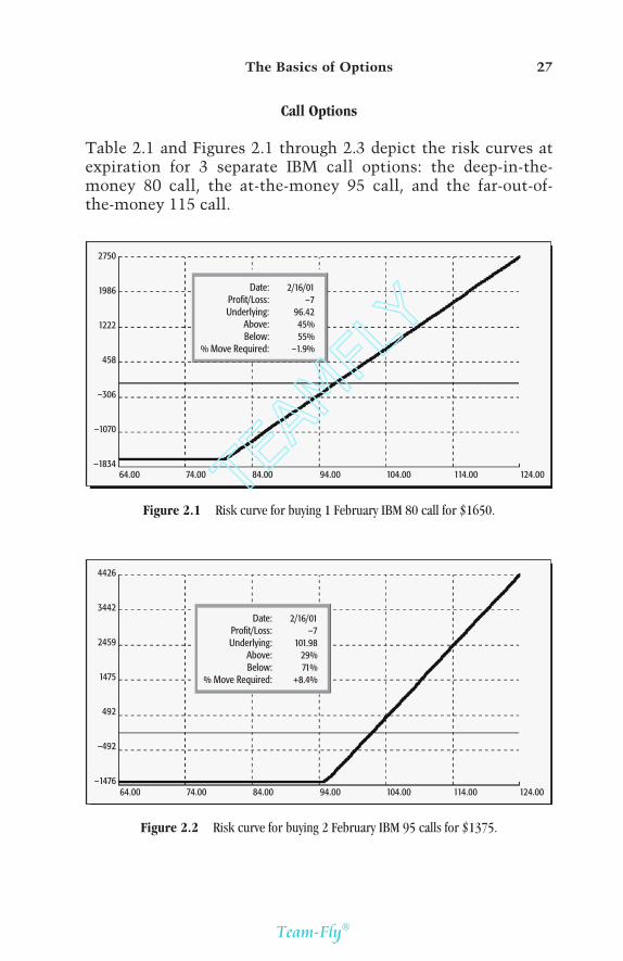
Table 2.1 and Figures 2.1 through 2.3 depict the risk curves atexpiration for 3 separate IBM call options: the deep-in-the-money 80 call, the at-the-money 95 call, and the far-out-of-the-money 115 call.
The Basics of Options 27
2750
1986
1222
458
–306
–1070
–183464.00 74.00 84.00 94.00 104.00 114.00 124.00
Date: 2/16/01 Profit/Loss: –7 Underlying: 96.42 Above: 45% Below: 55% % Move Required: –1.9%
Figure 2.1 Risk curve for buying 1 February IBM 80 call for $1650.
4426
3442
2459
1475
492
–492
–147664.00 74.00 84.00 94.00 104.00 114.00 124.00
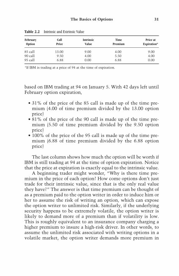
Date: 2/16/01 Profit/Loss: –7 Underlying: 101.98 Above: 29% Below: 71% % Move Required: +8.4%
Figure 2.2 Risk curve for buying 2 February IBM 95 calls for $1375.
TEAMFLY
Team-Fly®

Take a close look at the differences in the risk curves for thedeep-in-the-money February 80 call option and the far-out-of-the-money February 115 call option. Many traders are lured intobuying the inexpensive out-of-the-money option because of itslow price (a trader can buy thirteen 115 calls for about the samecost as one 80 call, which to some traders represents a deal theyjust can’t pass up). In fact, if IBM makes a big jump in price, thebuyer of the 115 calls stands to make almost four times as muchmoney on the same investment as the buyer of one 80 call. How-ever, the tradeoff here is that the stock must rise 24% by optionexpiration for the 115 call just to reach its break-even point. Thestock need only advance 1.9% or more by option expiration forthe 80 call to exceed its break-even point.
In sum, for the trader who expects IBM stock to rise in price,the 115 call offers the greater opportunity for making a great dealof money, whereas the 80 call offers a greater chance of makingany money.
Put Options
Figures 2.4 through 2.6 depict the risk curves for three separateIBM put options: the far-out-of-the-money 80 put, the at-the-money 95 put, and the deep-in-the-money 115 put.
28 The Option Trader’s Guide
10075
8116
6157
4198
2239
280
–168064.00 74.00 84.00 94.00 104.00 114.00 124.00
Date: 2/16/01 Profit/Loss: 7 Underlying: 116.17 Above: 7% Below: 93% % Move Required: +24.0%
Figure 2.3 Risk curve for buying 13 February IBM 115 calls for $1625.

Take a close look at the differences in the risk curves for thefar-out-of-the-money February 80 put option and the deep-in-the-money February 115 put option. Many traders are lured intobuying the inexpensive out-of-the-money option because of itslow price (a trader can buy nine 80 puts for the about the samecost as one 115 put, which to some traders represents a deal they
The Basics of Options 29
12267
6815
1363
–408964.00 74.00 84.00 94.00 104.00 114.00 124.00
Date: 2/16/01 Profit/Loss: 25 Underlying: 77.54 Above: 91% Below: 9% % Move Required: –17.5%
Figure 2.4 Buy 9 February IBM 80 puts for $2138.
7014
3897
779
–233864.00 74.00 84.00 94.00 104.00 114.00 124.00
Date: 2/16/01 Profit/Loss: 14 Underlying: 87.35 Above: 69% Below: 31% % Move Required: –7.1%
Figure 2.5 Buy 3 February IBM 95 puts for $2288.

just can’t pass up). In fact, if IBM stock declines dramatically, thebuyer of the 80 put stands to make more than four times asmuch money on the same investment as the buyer of one 115put. However, the tradeoff here is that the stock must decline–17.5% by option expiration for the 80 put to reach its break-even point. The stock need only decline –1.9% or more by optionexpiration for the 115 put to exceed its break-even point.
In sum, for the trader who truly expects IBM stock to fallsharply in price, the 80 put offers the greater opportunity formaking lots of money, whereas the 115 put offers a greaterchance of making any money.
Intrinsic Value versus Extrinsic Value
Table 2.2 shows the current price for several IBM call optionsand breaks the current price down into intrinsic value and ex-trinsic value. Column 1 shows the option’s strike price, Column2 shows the actual price of the option, Column 3 shows theamount of intrinsic value built into the price of the option, andColumn 4 shows the amount of extrinsic value—or time pre-mium—built into the current option price. These figures are
30 The Option Trader’s Guide
2888
1123
–642
–240764.00 74.00 84.00 94.00 104.00 114.00 124.00
Date: 2/16/01 Profit/Loss: –3 Underlying: 92.66 Above: 55% Below: 45% % Move Required: –1.9%
Figure 2.6 Buy 1 February IBM 115 put for $2138.
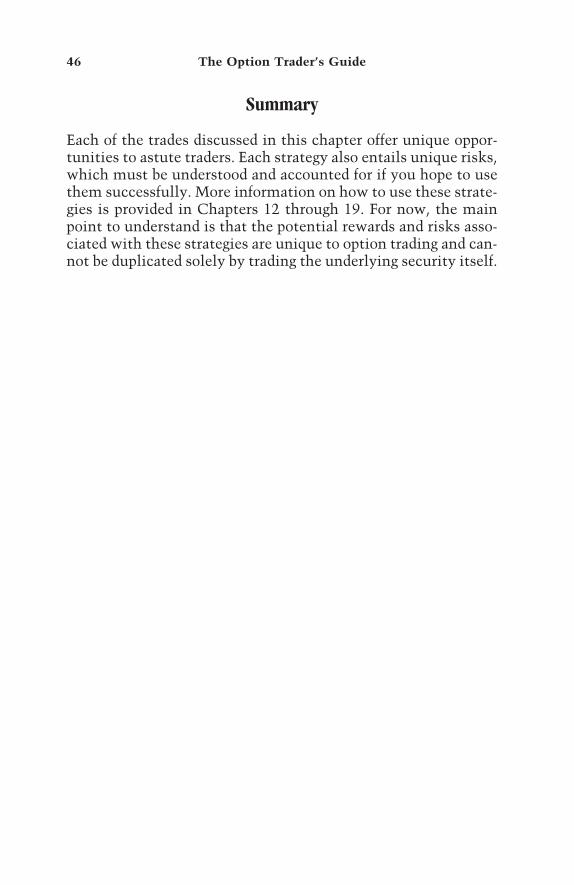
based on IBM trading at 94 on January 5. With 42 days left untilFebruary option expiration,
• 31% of the price of the 85 call is made up of the time pre-mium (4.00 of time premium divided by the 13.00 optionprice)
• 81% of the price of the 90 call is made up of the time pre-mium (5.50 of time premium divided by the 9.50 optionprice)
• 100% of the price of the 95 call is made up of the time pre-mium (6.88 of time premium divided by the 6.88 optionprice)
The last column shows how much the option will be worth ifIBM is still trading at 94 at the time of option expiration. Noticethat the price at expiration is exactly equal to the intrinsic value.
A beginning trader might wonder, “Why is there time pre-mium in the price of each option? How come options don’t justtrade for their intrinsic value, since that is the only real valuethey have?” The answer is that time premium can be thought ofas a premium paid to the option writer in order to induce him orher to assume the risk of writing an option, which can exposethe option writer to unlimited risk. Similarly, if the underlyingsecurity happens to be extremely volatile, the option writer islikely to demand more of a premium than if volatility is low.This is roughly equivalent to an insurance company charging ahigher premium to insure a high-risk driver. In other words, toassume the unlimited risk associated with writing options in avolatile market, the option writer demands more premium in
The Basics of Options 31
Table 2.2 Intrinsic and Extrinsic Value
February Call Intrinsic Time Price atOption Price Value Premium Expiration*
85 call 13.00 9.00 4.00 9.0090 call 9.50 4.00 5.50 4.0095 call 6.88 0.00 6.88 0.00
*If IBM is trading at a price of 94 at the time of expiration.

order to compensate for this risk. This is discussed in more detailin Chapters 4 through 6.
In-the-Money versus Out-of-the-Money Options
Which option a trader chooses to purchase has a significant im-pact on the cost of entry, the profit potential, and the probabilityof profit. Consider the following example. On January 5, a traderwith $3000 to invest expects IBM to rise before the February op-tion expiration. She considers the following choices:
• Buy 3 February 90 calls at 9.88 for $2962.• Buy 4 February 95 calls at 7.12 for $2850.• Buy 6 February 100 calls at 4.88 for $2925.
What are the implications for each choice? The best way toassess the relative advantages and disadvantages is to examinethe risk curves for each potential trade.
Figures 2.7 through 2.9 depict the risk curves for the three op-tions closest to the money—the 90, 95, and 100 strike prices—with IBM trading at a price of 94.
32 The Option Trader’s Guide
6038
4529
3019
1510
0
–1510
–302068.00 76.69 85.31 94.00 102.69 111.31 120.00
Date: 2/16/01 Profit/Loss: –22 Underlying: 99.88 Above: 27% Below: 73% % Move Required: +6.2%
Figure 2.7 Risk curve for buying 3 February 90 calls at 9.88.

Table 2.3 displays the break-even price for each trade, thepercentage move required to reach the break-even point, and theprobability of that price level being reached at the time of optionexpiration. The obvious trend to note is that the further out-of-the-money the strike price of the option is, the lower the proba-bility of generating a profit.
The Basics of Options 33
7152
5364
3576
1788
0
–1788
–357668.00 76.69 85.31 94.00 102.69 111.31 120.00
Date: 2/16/01 Profit/Loss: –26 Underlying: 102.04 Above: 21% Below: 79% % Move Required: +8.4%
Figure 2.8 Risk curve for buying 4 February 95 calls at 7.12.
9078
5043
1009
–302668.00 76.69 85.31 94.00 102.69 111.31 120.00
Date: 2/16/01 Profit/Loss: 19 Underlying: 104.93 Above: 13% Below: 87% % Move Required: +11.8%
Figure 2.9 Risk curve for buying 6 February 100 calls at 4.88.

Table 2.4 displays the expected dollar and percentage returnfor each trade based on different movements in the underlyingstock. From the returns displayed in this example we can makethe following observations:
• If you are highly confident that the stock is going to explodesharply higher, the February 100 call offers the greatest lever-age if your opinion turns out to be correct.
• The February 90 call is the only option (in this example) thatwill not lose 100% if the stock is unchanged at expiration. Inaddition, if the stock rises 15% or even 30%, the 90 call willoutperform the 95 call.
• In sum, the February 100 call offers the greatest profit poten-tial, and the February 90 call offers the most favorable trade-off between reward and risk.
From all the information presented on these three trades,there is no way to state definitively that one trade is better thanthe other. Just as beauty is in the eye of the beholder, the crite-ria that make a given trade more attractive than another vary
34 The Option Trader’s Guide
Table 2.3 Break-Even Analysis
Stock Break-Even Percentage Probability ofTrade Entered Price Move Required Reaching Break-Even
Buy 3 February 90 calls at 9.88 99.88 +6.2% 27%Buy 4 February 95 calls at 7.12 102.12 +8.4% 21%Buy 6 February 100 calls at 4.88 104.88 +11.8% 13%
Table 2.4 Expected Returns
Stock Down Stock Down Stock Stock Up Stock UpTrade Entered –30% –15% Unchanged +15% +30%
Buy 3 February –$2962 –$2962 –$1762 +$2467 +$6698 90 calls at 9.88 (–100%) (–100%) (–59%) (+83%) (+126%)
Buy 4 February –$2850 –$2850 –$2850 +$2390 +$6023 95 calls at 7.12 (–100%) (–100%) (–100%) (+84%) (+111%)
Buy 6 February –$2925 –$2925 –$2925 +$1935 +$10395 100 calls at 4.88 (–100%) (–100%) (–100%) (+66%) (+255%)

from trader to trader. Nevertheless, regardless of which tradeyou might choose, the key to success remains the same. Thetrader who will succeed in the long run is the one who takesthe time to analyze the various risk-versus-reward characteris-tics of several potential trades and then chooses the trade thatbest matches his or her particular objective for that trade.
Summary
In any field of endeavor, a thorough understanding of the basicsis a prerequisite to success. If you are new to option trading, youshould take the time to review the material in this chapter thor-oughly. Once you have a firm handle on the basics, the materialin the following chapters will flow much more easily and the relevance of each concept will be much more obvious as youproceed.
The Basics of Options 35


Chapter 3
REASONS TO TRADE OPTIONS
37
Because they trade based on the price action of some underlyingsecurity, be it a stock, a stock index, or a futures contract,options are referred to as derivatives. In other words, their char-acteristics derive from the price action of the underlying secu-rity. As a result, although the action of the options for a givenunderlying security are related to the underlying, options offermany unique opportunities that cannot be attained solelythrough trading the underlying security.
Before getting into the nitty-gritty of option trading, let’sexamine the bigger picture. The first question on the table is not“How should I trade options?” but rather “Why bother with op-tions in the first place?” In other words, what qualities of optionsare so valuable that a trader should consider using options ratherthan simply sticking to stocks, bonds, futures, and mutualfunds?
Options offer a number of extremely useful advantages overother forms of investment. At the same time, it should not be as-sumed that you should therefore ignore traditional investmentsand commit all your capital to option trading—quite the oppo-site. Options are best used to augment your other investments.
The Three Primary Uses of Options
There are three primary uses of options. Each of these uses offerunique benefits—and risks—that traders and investors cannot
TEAMFLY
Team-Fly®

obtain from traditional investment vehicles. The three primaryuses of options follow.
1. Leveraging an opinion on market direction. Buying an op-tion gives a trader the ability to control 100 shares of stock orone futures contract, usually for far less money than it wouldcost to trade the underlying security outright. If a trader’s timingis right when entering into an option trade, he or she can obtaina much higher percentage rate of return than by simply tradingthe underlying while risking fewer investment dollars. By buy-ing a naked option a trader can potentially make the same dollarprofit, and a much greater percentage return, than he or she mightby committing the capital to buy or sell short the underlyingsecurity itself.
2. Hedging an existing position (or generating income from astock portfolio). At times traders may wish to temporarily min-imize or eliminate the downside risk associated with a positionthey presently hold without completely exiting the current po-sition altogether. This process—referred to as hedging an exist-ing position—can be accomplished in several different waysusing options. One alternative is to buy one put option for every100 shares of stock (or every futures contract) held. Another al-ternative many investors engage in is covered call writing, whichreduces downside risk to a certain degree and can increase an in-vestor’s income. Covered call writing is discussed in more detailin Chapter 18.
3. Taking advantage of neutral situations. Taking advantage ofneutral situations is an area that is entirely unique to optiontrading. If you buy a stock or a futures contract, that securitymust rise in price in order for you to profit. If you sell short astock or sell short a futures contract, the price of that securitymust fall for you to profit. With the use of options, you can enterpositions that can benefit from a security rising or falling and po-sitions that benefit from a security remaining in a particularprice range for a certain period. Some examples of these types ofstrategies are calendar spreads (see Chapter 14), straddles (seeChapter 15), vertical spreads (see Chapter 16), and butterflyspreads (see Chapter 19).
38 The Option Trader’s Guide

Leveraging an Opinion on Market Direction
The most common use of options is to leverage the amount ofprofit possible from an anticipated move by a given stock, stockindex, or futures contract. Buying a call or a put option can allowa trader to
• Put up less money than would be needed to buy or sell short100 shares of stock or to go long or short a futures contract
• Earn a much greater percentage return on a trade than wouldresult from buying or selling short 100 shares of stock orgoing long or short a futures contract
To buy an option, a trader pays a premium to the optionwriter. The amount paid to buy the option represents the optionbuyer’s total risk on the trade. Conversely, upside potential isunlimited. The mantra of “limited risk, unlimited profit poten-tial” is an oft-quoted and technically accurate description. Nev-ertheless, as discussed in Chapter 1, there are tradeoffs associatedwith every potential option trade.
For the sake of example, let’s consider a trader who expectsthe price of IBM stock to rise. With the stock trading at 94, thetrader can simply buy the stock or buy a call option. Because hewants a position that is roughly equivalent to 100 shares ofstock, he may consider the following possible trades:
• Buy 100 shares of IBM at 94 a share for $9400.• Buy 2 IBM 95 call options at 7.12 for $1425.
Table 3.1 depicts the expected dollar and percentage returnsthat would be achieved depending on the movement of the un-derlying security.
Figures 3.1 and 3.2 depict graphically the expected profit orloss for both of these positions. Consider the tradeoffs involvedin choosing between the trades shown in Figure 3.1. In this ex-ample, extreme moves in either direction favor the option trader.If the stock goes up 20%, the option trader will actually experi-ence a larger dollar gain than the stock trader despite putting uponly 15% as much capital as the stock trader. Also, if the stock
Reasons to Trade Options 39

40 The Option Trader’s Guide
Table 3.1 Expected Returns at Different Price Levels
Buy 100 Shares Buy Two 95 Call OptionsChange in Stock Price Cost: $9400 Cost: $1425
Stock up 20% +$1880 (+20%) +$2135 (+149%)Stock up 10% +$940 (+10%) +$128 (+9%)Stock unchanged 0% –$1425 (–100%)Stock down 10% –$940 (–10%) –$1425 (–100%)Stock down 20% –$1880 (–20%) –$1425 (–100%)
2000
667
–667
–200074.00 80.69 87.31 94.00 100.69 107.31 114.00
Date: 2/16/01 Profit/Loss: 3 Underlying: 94.09 Above: 47% Below: 53% % Move Required: +0.4%
Figure 3.1 Risk curve for buying 100 shares of IBM stock at 94.
2350
1045
–261
–156774.00 80.69 87.31 94.00 100.69 107.31 114.00
Date: 2/16/01 Profit/Loss: –6 Underlying: 102.28 Above: 27% Below: 73% % Move Required: +9.1%
Figure 3.2 Risk curve for buying 2 IBM February 95 call options at 7.12.

drops 20%, the stock trader would be $1880 in the hole. Con-versely, the option trader can lose no more than the $1425 he in-vested in the trade. This is true even if the stock dropped 30%,40%, 50%, or more. Clearly, a trader who wants to maximizeprofitability and who is extremely confident that the stock isgoing to advance would want to choose the option trade.
On the other hand, if the stock stays within a narrow rangethrough option expiration, the stock trader will come out ahead.The most dramatic example occurs if the stock is unchangedand closes at 94 on the day of option expiration. In this event, thestock trader would have no gain or loss, but the option traderwould lose the entire $1425 investment on the trade.
This example clearly illustrates the tradeoffs involved in de-ciding whether to buy stock or a call option.
Hedging an Existing Position (and Generating Income)
Another unique and very popular use of options is to hedge anexisting position. At times investors may be concerned aboutshort-term downside risk but for various reasons (for example,tax implications) do not want to sell their positions in the un-derlying security. By using an option strategy, investors can re-duce or even completely eliminate any downside risk beyond acertain point. To do so, investors must invariably give up someupside profit potential, at least in the short term.
Possibly the most commonly used option trading strategy,after simply buying naked calls and puts, is known as coveredcall writing. This strategy is detailed in Chapter 18, but we willdiscuss it here briefly. A trader writes a covered call by sellingshort, that is, writing a call option on a stock (or futures con-tract) that she already holds. By writing this option, the trader
• Receives the option premium, which is hers to keep whetherthe stock goes up or down
• In effect agrees to sell 100 shares of stock (or one futures con-tract) at the option’s strike price, even if the stock rises abovethe strike price
• Retains the right to buy back the option (possibly at a loss) ifshe does not want the stock to get called away
Reasons to Trade Options 41

Consider the following example. Trader A holds 100 sharesof IBM stock, which is presently trading at 94. Trader B alsoholds 100 shares of stock and decides to write a covered call. Hewrites one February 100 call option and receives a price of 4.50,or $450. If IBM is trading at 100 or below as of option expiration,the trader will keep the entire $450 premium received. To betterappreciate the allure of writing covered calls, consider this: If atrader could execute this trade four times per year, he couldpotentially generate up to $1800 worth of income. This repre-sents a 19.1% return even if the stock price remains unchanged.
Trader A holds 100 shares of IBM at 94 for $9400.Trader B holds 100 shares of IBM at 94, sells 1 IBM 100 call
option at 4.50.
Table 3.2 depicts the expected dollar and percentage returnsthat would be achieved depending on the movement of the un-derlying security.
Notice the tradeoffs involved in choosing between thesetrades. In this example, a sharp rise in the price of IBM stock fa-vors Trader A because Trader B, by virtue of selling a call with astrike price of 100—thereby agreeing to sell his stock at thatprice—gives up any profit potential above a price of 100. Never-theless, if the stock were called away, Trader B would still earnan 11% return in 42 days or less, which represents an attractiveannualized rate of return. If the stock stays in a narrow range,Trader B comes out ahead by virtue of having taken in the optionpremium of $450. If the stock falls, Trader B will always comeout at least slightly ahead of Trader A, once again by virtue of
42 The Option Trader’s Guide
Table 3.2 Expected Returns at Different Price Levels
Change in Stock Price Buy 100 Shares Buy 100 Shares, Short 1 Call
Stock up 20% +$1880 (+20%) +$1050 (+11%)Stock up 10% +$940 (+10%) +$1050 (+11%)Stock unchanged 0% +$450 (+6%)Stock down 10% –$940 (–10%) –$490 (–5%)Stock down 20% –$1880 (–20%) –$1430 (–15%)

having received the option premium of $450. Nevertheless, ifthe stock falls too far, both traders will face the prospect of alarge loss and may need to act in order to cut the loss. The bot-tom line is that as a hedging strategy, covered call writing offersonly limited downside protection (see Figures 3.3 and 3.4).
Reasons to Trade Options 43
1292
345
–603
–155074.00 80.69 87.31 94.00 100.69 107.31 114.00
Date: 2/16/01 Profit/Loss: 29 Underlying: 89.73 Above: 63% Below: 37% % Move Required: –4.7%
Figure 3.4 Risk curve for buying 100 shares of IBM stock at 94 and writing 1 February100 call option at 4.50.
2000
667
–667
–200074.00 80.69 87.31 94.00 100.69 107.31 114.00
Date: 2/16/01 Profit/Loss: 3 Underlying: 94.09 Above: 47% Below: 53% % Move Required: +0.4%
Figure 3.3 Risk curve for buying 100 shares of IBM stock at 94.

Taking Advantage of Neutral Situations
A unique use of options involves taking advantage of neutral sit-uations, that is, situations whereby a trader makes money basedon an underlying security remaining within a particular pricerange, or conversely, making a large move either up or down.This type of opportunity is available only to option traders. Ifyou buy a stock or futures contract and its price remains un-changed, you neither make money nor lose money. Conversely,by using one of several option strategies, you can conceivablyearn a high rate of return even while the price of the underlyingsecurity remains in a narrow range.
One example of a neutral strategy is known as a calendarspread. To establish a calendar spread an option trader buys a call(or put) option in a further-off expiration month and simultane-ously writes an option with the same strike price for a nearer-term month. This strategy is covered in detail in Chapter 14, butthe basic idea is that the near-term option loses value morequickly than the longer-term option, thus generating a profit.
As an example of a calendar spread, you could buy the April95 IBM call option at a price of 10.50 and simultaneously writethe February 95 IBM call option at a price of 6.75. To enter thistrade you would pay the difference in price of 3.75 points, or$375. To buy a 10-lot of this spread would cost $3750. Let’s com-pare this position to holding 100 shares of stock purchased at $94a share.
Table 3.3 shows the expected dollar and percentage returnsthat would be achieved depending on the movement of the un-derlying security.
44 The Option Trader’s Guide
Table 3.3 Expected Returns at Different Price Levels
Buy 10 April 100 CallsBuy 100 Shares Sell 10 February 100 Calls
Change in Stock Price Cost: $9400 Cost: $3750
Stock up 20% +$1880 (+20%) –$560 (–15%)Stock up 10% +$940 (+10%) +$1590 (+42%)Stock unchanged 0% +$4080 (+109%)Stock down 10% –$940 (–10%) –$70 (–2%)Stock down 20% –$1880 (–20%) –$2430 (–65%)

Notice the stark contrast in returns for these two positions ateach price level. Whereas the long stock position makes moneyif the stock rises and loses money if the stock falls, the optionposition
• Makes money if the stock remains relatively unchanged• Incurs losses if the stock makes a significant move in either
direction (see Figures 3.5 and 3.6)
Reasons to Trade Options 45
2000
667
–667
–200074.00 80.69 87.31 94.00 100.69 107.31 114.00
Date: 2/16/01 Profit/Loss: 3 Underlying: 94.09 Above: 47% Below: 53% % Move Required: +0.4%
Figure 3.5 Risk curve for buying 100 shares of IBM stock at 94.
4550
3290
2020
760
–510
–1770
–304074.00 80.69 87.31 94.00 100.69 117.31 114.00
Date: 2/16/01 Profit/Loss: 4080 Underlying: 94.04 Above: 47% Below: 53% % Move Required: +0.4%
Figure 3.6 Risk curve for buying 10 April 100 calls and writing 10 February 100 Calls.
Summary
Each of the trades discussed in this chapter offer unique oppor-tunities to astute traders. Each strategy also entails unique risks,which must be understood and accounted for if you hope to usethem successfully. More information on how to use these strate-gies is provided in Chapters 12 through 19. For now, the mainpoint to understand is that the potential rewards and risks asso-ciated with these strategies are unique to option trading and can-not be duplicated solely by trading the underlying security itself.
46 The Option Trader’s Guide

Chapter 4
OPTION PRICING
47
The price for a given option in the marketplace is determinedprimarily by supply and demand. In other words, unless a buyerand a seller of a particular option are willing to consummate atrade at an agreed-on price, there is no trade. As discussed inChapter 9, when you actually go to enter a trade you are quoteda bid price and an ask price. If you want to buy an option at thecurrent market price, you pay the ask price. If you want to sell anoption at the current market price, you receive the bid price.These bid and ask prices are generally quoted by traders knownas market makers, who make their living by buying and sellingoptions for a given security or group of securities.
For stock options the spread between the bid and ask pricecan range anywhere from one-eighth of a point to a full point ormore. This spread can have a profound effect on your actual trad-ing results. The size of this spread varies based on such factors asvolume, volatility, and the raw price of the option itself. If an op-tion on a $25 stock is 20 points out of the money, the price of theoption will be very low and so will the bid-ask spread. Generally,the more actively traded an option, the tighter the bid-askspread. Conversely, an option that is 20 points in the moneymay be bid at a price of 21 and offered at a price of 22.
Theoretical Value
In most cases the market price for an option is slightly above toslightly below the theoretical price for that option, which is also
TEAMFLY
Team-Fly®

referred to as fair value. In the early days of option trading, therewas no such thing as fair value. The market makers for the op-tions on a particular security would set a price and other traderscould either pay this price or simply not trade. Eventually sev-eral scholars got together and developed a formula for determin-ing a fair price for a given option, based on a set of currentvariables.
The most commonly used model is the Black-Scholes model,named after its developers. Another commonly used optionmodel is the binomial model, which uses a complex series ofiterative calculations to arrive at its version of fair value for agiven option. There are several other variations, but by and largethe theoretical prices calculated by various option models aregenerally very close in value. In each case, the inputs used to de-termine an option’s theoretical price are roughly the same:
A. The current price of the underlying securityB. The strike price of the option under analysisC. Current interest ratesD. The number of days until the option expiresE. A volatility value
Elements A through E are passed to an option pricing model,which then generates a theoretical option price. (Note that stockdividends also play a role in option models, but this element isomitted here for simplicity.)
Elements A, B, C, and D are known variables. In other words,at any given point in time one can readily observe the underly-ing price, the strike price for the option in question, the currentlevel of interest rates, and the number of days until the optionexpires. In selecting a volatility value to use in the option modelcalculation, the most commonly used choice is the actual his-toric volatility of the underlying security. Historical volatility isdiscussed in more detail in Chapter 6, but in general terms, his-toric volatility measures the standard deviation of underlyingprice changes during a given period in order to calculate an esti-mate of how much that security is likely to rise or fall within thenext 12 months. For example, a stock with a historical volatility
48 The Option Trader’s Guide

of 30 would be expected to rise or fall within a range of plus orminus 30% in the next 12 months. Similarly, a stock with a his-torical volatility of 80 would be expected to rise or fall within arange of plus or minus 80% in the next 12 months.
As will become more clear between here and the end ofChapter 8, the level of volatility inherent in the underlying se-curity has a profound effect on the prices for options on thatsecurity.
Examples of Theoretical Option Pricing
The following example illustrates the factors that go into calcu-lating a theoretical option price. Let’s assume the following vari-ables for a particular underlying stock:
Current date February 12, 2001Current price of the underlying security 99Strike price of the option under analysis 100Current interest rate 5Number of days until the option expires 33Volatility 30
Given these inputs, the Black-Scholes option model wouldreturn the following theoretical call and put prices for the March2001 100 call and put options:
Theoretical 100 call price 3.32Theoretical 100 put price 3.92
Table 4.1 uses the same variables as the previous example,except for the volatility value. Table 4.1 shows the theoreticalprice for both the 100 call and put options for five differentvolatility levels. Volatility is increased from 10 to 50 in incre-ments of 10, with all other variables held constant. Note theprofound effect these changes in volatility have on the theoreti-cal option prices calculated by the option model.
Option Pricing 49

Table 4.2 displays the theoretical and actual market pricesand the difference between the two for IBM options on January 5.Note that the options with strike prices closest to the currentstock price—the 90, 95, and 100 strike price options—show thesmallest difference between theoretical and actual prices. This isa common phenomenon because the near-the-money optionstend to have the greatest volume and so tend to be the most ac-curately priced options for each security.
Overvalued Options versus Undervalued Options
If the actual market price for an option is above the theoreticalprice for that option, that option is considered overvalued. Intheory, a trader can gain a slight edge by writing options that areovervalued. Conversely, if the actual market price of an option isbelow the theoretical price for that option, that option is consid-ered undervalued. In theory, a trader gains a slight edge by buy-ing options that are undervalued and/or writing options that areovervalued. Traders should be forewarned, however, not to ex-pect to make a living buying undervalued options and writingovervalued options. Many other factors are involved that canquickly wipe out any theoretical edge. For example, if a traderbuys an undervalued call and the underlying stock subsequentlyplummets, that option is going to decline in price anyway.
In Table 4.2, overvalued options are noted by a negative Diff.value (differential) and undervalued options are noted by a posi-tive Diff. value.
50 The Option Trader’s Guide
Table 4.1 The Effect of Volatility on Theoretical Option Prices
Underlying Strike Interest Days to Theoretical Theoretical Price Price Rate Expiration Volatility Call Price Put Price
99 100 5 33 10 0.93 1.5599 100 5 33 20 2.14 2.7399 100 5 33 30 3.32 3.9299 100 5 33 40 4.51 5.1099 100 5 33 50 5.69 6.28
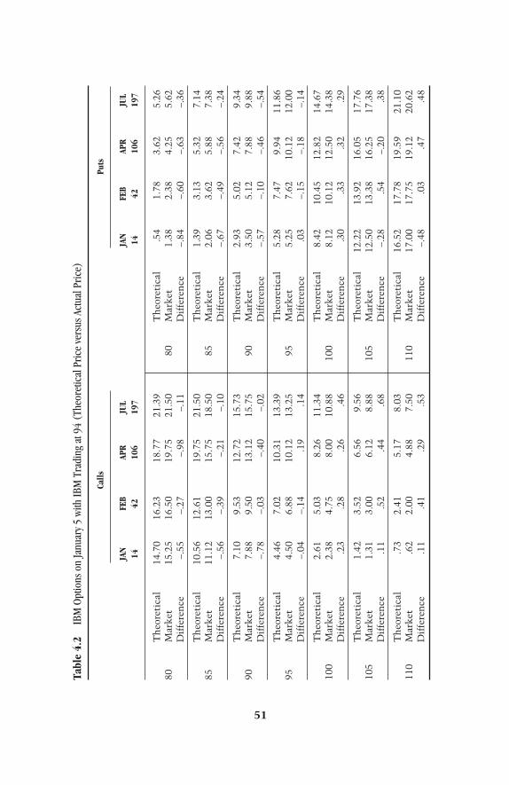
51
Tabl
e 4.
2IB
M O
ptio
ns o
n Ja
nuar
y 5
with
IBM
Tra
ding
at 9
4 (T
heor
etic
al P
rice
ver
sus
Actu
al P
rice
)
Calls
Puts
JAN
FEB
APR
JUL
JAN
FEB
APR
JUL
1442
106
197
1442
106
197
Th
eore
tica
l14
.70
16.2
318
.77
21.3
9T
heo
reti
cal
.54
1.78
3.62
5.26
80M
ark
et15
.25
16.5
019
.75
21.5
080
Mar
ket
1.38
2.38
4.25
5.62
Dif
fere
nce
–.55
–.27
–.98
–.11
Dif
fere
nce
–.84
–.60
–.63
–.36
Th
eore
tica
l10
.56
12.6
119
.75
21.5
0T
heo
reti
cal
1.39
3.13
5.32
7.14
85M
ark
et11
.12
13.0
015
.75
18.5
085
Mar
ket
2.06
3.62
5.88
7.38
Dif
fere
nce
–.56
–.39
–.21
–.10
Dif
fere
nce
–.67
–.49
–.56
–.24
Th
eore
tica
l7.
109.
5312
.72
15.7
3T
heo
reti
cal
2.93
5.02
7.42
9.34
90M
ark
et7.
889.
5013
.12
15.7
590
Mar
ket
3.50
5.12
7.88
9.88
Dif
fere
nce
–.78
–.03
–.40
–.02
Dif
fere
nce
–.57
–.10
–.46
–.54
Th
eore
tica
l4.
467.
0210
.31
13.3
9T
heo
reti
cal
5.28
7.47
9.94
11.8
695
Mar
ket
4.50
6.88
10.1
213
.25
95M
ark
et5.
257.
6210
.12
12.0
0D
iffe
ren
ce–.
04–.
14.1
9.1
4D
iffe
ren
ce.0
3–.
15–.
18–.
14
Th
eore
tica
l2.
615.
038.
2611
.34
Th
eore
tica
l8.
4210
.45
12.8
214
.67
100
Mar
ket
2.38
4.75
8.00
10.8
810
0M
ark
et8.
1210
.12
12.5
014
.38
Dif
fere
nce
.23
.28
.26
.46
Dif
fere
nce
.30
.33
.32
.29
Th
eore
tica
l1.
423.
526.
569.
56T
heo
reti
cal
12.2
213
.92
16.0
517
.76
105
Mar
ket
1.31
3.00
6.12
8.88
105
Mar
ket
12.5
013
.38
16.2
517
.38
Dif
fere
nce
.11
.52
.44
.68
Dif
fere
nce
–.28
.54
–.20
.38
Th
eore
tica
l.7
32.
415.
178.
03T
heo
reti
cal
16.5
217
.78
19.5
921
.10
110
Mar
ket
.62
2.00
4.88
7.50
110
Mar
ket
17.0
017
.75
19.1
220
.62
Dif
fere
nce
.11
.41
.29
.53
Dif
fere
nce
–.48
.03
.47
.48

Table 4.3 displays the expected theoretical price for the IBMFebruary 95 call option over one period and through a range ofunderlying prices. For this display, volatility and interest ratesare held constant. The range of stock prices is listed down theleft side of the grid and the number of days left until expirationacross the top of the grid. Note that as the underlying price in-creases, so does the option price. Conversely, as the price of thestock falls, so does the price of the option. Notice how the optionprice decreases (or decays) with the passage of time, even if theunderlying price is held constant. This is an illustration of timedecay, which is discussed in greater detail in Chapter 5.
Summary: Theory versus Reality
It is important to understand how options are priced and to beable to recognize if a particular option is overvalued (i.e., tradingabove its theoretical value) or undervalued (i.e., trading below itstheoretical value). Nevertheless, in the real world of trading thisinformation often becomes somewhat moot. For instance, sup-pose you are bullish on a given stock and have selected a call op-tion that you want to buy. Just before you place an order to buythe option you realize that the ask price for the option is 5.00,but according to your option pricing model the theoretical priceor fair value for the option is only 4.25. Now you are faced with
52 The Option Trader’s Guide
Table 4.3 Theoretical Prices for 95 Call (Current Option Price = 6.5, Current UnderlyingPrice = 94)
Days until Expiration
37 32 27 22 17 12 7 2
112.81 20.00 19.63 19.25 18.94 18.56 18.25 18.00 17.88108.12 16.13 15.69 15.25 14.81 14.38 13.88 13.44 13.19103.43 12.56 12.13 11.63 11.06 10.50 9.88 9.19 8.5698.68 9.38 8.88 8.31 7.75 7.13 6.38 5.50 4.3894.00 6.69 6.19 5.63 5.06 4.38 3.69 2.75 1.5089.31 4.50 4.00 3.50 3.00 2.44 1.81 1.06 0.2584.62 2.81 2.38 2.00 1.56 1.19 0.75 0.31 0.0079.93 1.56 1.31 1.00 0.75 0.44 0.25 0.06 0.0

a choice. Do you pay a price that is theoretically too high for theoption, or do you skip the trade altogether? If you buy the optionanyway and the underlying security fails to make a big move,you will suffer an even bigger loss than you would if you hadbeen able to buy the option at fair value. If you skip the trade al-together and the underlying security makes the huge move youexpected, you will have missed out on a large profit for fear ofrisking a few dollars more.
In sum, it is important to be aware of the price of a given op-tion in the marketplace relative to the fair value calculated forthat option by an option pricing model. However, in the realworld the currently available bid and ask prices have a muchgreater impact on your success or failure than the theoreticalvalue for a given option.
Option Pricing 53


Chapter 5
TIME DECAY
55
If an option is trading in the money before expiration, the priceof that option comprises intrinsic value plus time premium. If anoption is trading out of the money before expiration, the price ofthat option is made up solely of time premium.
The amount of time premium built into the price of anygiven option depends on the option pricing variables discussed inChapter 4. In other words, the amount of time left until expira-tion, the volatility, the amount by which the option is in or outof the money, and the current level of interest rates are all fac-tors influencing the amount of time premium built into the priceof each option.
The time premium built into any option decays at an everfaster rate as option expiration draws nearer. Most commonlyreferred to as time decay, this phenomenon can have a profoundeffect on many option trades that a trader might consider.
As a trader it is important to understand and accept the factthat once an option reaches expiration, there will be no timepremium left in its price. If the option is trading in the money atthe time of expiration, the price of that option will be equal tothe difference between the price of the underlying stock or fu-tures market and the strike price of the option. If the option istrading out of the money at the time of expiration, it will beworthless.
Because of this mathematical fact we can state that there arethree great certainties in life:

• Death.• Taxes.• Every option will lose all of its time premium at expiration.
Understanding the effect that time decay can have on eachtrade you make is one of the keys to consistently putting theodds on your side trade after trade. Traders who are not con-cerned about time decay are almost certain to fail in the long runbecause too often they will be betting on a long shot—oftenwithout even knowing they are doing so. Although this maysound foreboding to some, the underlying concept is extremelysimple:
• If you buy premium, time premium decay works against you.• If you sell premium, time premium decay works for you.
This is not to imply that you should always write options orthat you should never buy options. What it means is that if youhope to succeed in option trading, you must understand thesetwo tenets and take steps to maximize the potential benefits andminimize the potential negative effect that time decay can haveon your option positions.
The best way to illustrate the effect and importance of timedecay is with an example. Let us assume the following hypo-thetical situation. On August 18, the stock of IBM is trading at aprice of 120. A trader wishes to buy the October 120 call, whichhas 63 days left until expiration. The price of the option pur-chased is 8.44. For the sake of argument—and to highlight timedecay as the only key variable in this example—we assume thatat the end of each subsequent week IBM is still trading at a priceof 120 and that volatility is unchanged.
The Effect of Time Decay on the Price of an Option
Table 5.1 and Figures 5.2 and 5.3 each show the effect of timedecay on the price of the IBM October 120 call in a slightly dif-ferent format. Table 5.1 displays numerically the expected priceof the option at the end of each week as well as the percentage
56 The Option Trader’s Guide
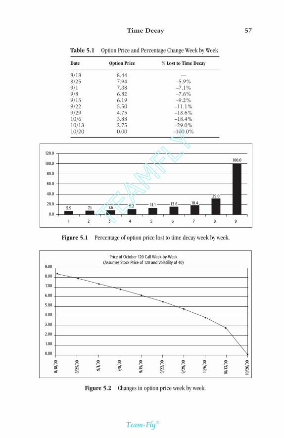
Time Decay 57
Table 5.1 Option Price and Percentage Change Week by Week
Date Option Price % Lost to Time Decay
8/18 8.44 —8/25 7.94 –5.9%9/1 7.38 –7.1%9/8 6.82 –7.6%9/15 6.19 –9.2%9/22 5.50 –11.1%9/29 4.75 –13.6%10/6 3.88 –18.4%10/13 2.75 –29.0%10/20 0.00 –100.0%
120.0
100.0
80.0
60.0
40.0
20.0
0.0
1 2 3 4 5 6 7 8 9
5.9 7.1 7.6
100.0
13.6 18.411.19.2
29.0
Figure 5.1 Percentage of option price lost to time decay week by week.
Price of October 120 Call Week-by-Week(Assumes Stock Price of 120 and Volatility of 40)
9.00
8.00
7.00
6.00
5.00
4.00
3.00
2.00
1.00
0.00
8/18
/00
8/25
/00
9/1/
00
9/8/
00
9/15
/00
9/22
/00
9/29
/00
10/6
/00
10/1
3/00
10/2
0/00
Figure 5.2 Changes in option price week by week.
TEAMFLY
Team-Fly®
loss from the previous week’s closing price. Figure 5.1 shows thepercentage loss from the previous week’s closing price in graph-ical form. Figure 5.2 shows the price of the option at the end ofeach week. The key elements to note are these:
• Time decay is an inevitable and progressive process.• The rate at which the time premium in an option price de-
cays accelerates as expiration draws nearer.
Implications of Time Decay
There are several implications of time decay that a trader mustrecognize and account for when planning and executing trades.Most notably, if you buy an option, you must expect to lose aportion of the price of your option as time goes by. You musthope that the underlying security moves far enough in the direc-tion that you expect it to in order to compensate for this loss oftime premium. If you are an option writer, you can expect timedecay to work in your favor as time goes by. As an option writer,your primary concern is that the underlying price will moveagainst you and create losses in excess of the amount you gainfrom time decay.
Time Decay Illustrated
Although a textbook understanding of time decay and its effecton the price of an option may be interesting and important, for atrader it is most important to understand the effect it will haveon a given trade. The net effect of time decay to you as an optionbuyer is that with each passing day and week, the break-evenprice for your trade moves further away.
Figures 5.3 through 5.7 illustrate the negative effect of timedecay for the option buyer. Notice how each successive riskcurve moves slightly lower and farther to the right (i.e., thebreak-even price moves a little further away each week) as someof the time premium paid by the option buyer evaporates. This
58 The Option Trader’s Guide

Time Decay 59
1406
1015
625
234
–156
–547
–938100.00 106.69 113.31 120.00 126.69 133.31 140.00
Date: 8/25/00 Profit/Loss: –4 Underlying: 121.06 Above: 43% Below: 57% % Move Required: +1.0%
Figure 5.3 IBM October 120 call as of 8/25/00.
1328
959
590
221
–147
–516
–886100.00 106.69 113.31 120.00 126.69 133.31 140.00
Date: 9/08/00 Profit/Loss: –4 Underlying: 122.88 Above: 40% Below: 60% % Move Required: +2.3%
Figure 5.4 IBM October 120 call as of 9/8/00.
means that for each week that passes, the probability of reachingthe break-even price declines slightly.
A key point to note (see Figure 5.8) is that if you buy an op-tion, you will make more money if the underlying security’sprice rises sooner rather than later. In this example, if IBM shot

up from 120 to 140 in one week, the buyer of this option wouldexpect to have a profit of $1406. Conversely, if the stock rises to140 by expiration on October 20, the profit would be only $1156.
Table 5.2 illustrates numerically the negative effect of timedecay. Assuming that as of each date, the price of IBM stock is
60 The Option Trader’s Guide
1252
904
556
209
–139
–487
–835100.00 106.69 113.31 120.00 126.69 133.31 140.00
Date: 9/22/00 Profit/Loss: –3 Underlying: 124.76 Above: 38% Below: 62% % Move Required: +3.7%
Figure 5.5 IBM October 120 call as of 9/22/00.
1188
825
462
99
–264
–627
–990100.00 106.69 113.31 120.00 126.69 133.31 140.00
Date: 10/06/00 Profit/Loss: 0 Underlying: 127.05 Above: 35% Below: 65% % Move Required: +5.7%
Figure 5.6 IBM October 120 call as of 10/6/00.

120, notice how time decay in the price of the option causes thebreak-even price to move farther away. Thus, with each passingweek, the percentage move required for the stock to reach thebreak-even price increases and the probability of reaching the pricedeclines.
Time Decay 61
1156
803
449
96
–257
–610
–964100.00 106.69 113.31 120.00 126.69 133.31 140.00
Date: 10/20/00 Profit/Loss: 0 Underlying: 128.55 Above: 34% Below: 66% % Move Required: +7.1%
Figure 5.7 IBM October 120 call as of 10/20/00.
1406
1015
625
234
–156
–547
–938100.00 106.69 113.31 120.00 126.69 133.31 140.00
Date: 10/20/00 Profit/Loss: 5 Underlying: 128.47 Above: 34% Below: 66% % Move Required: +7.1%
Figure 5.8 IBM October 120 call (the effect of time decay).

Summary
Time decay is a factor involved in virtually every single optiontrade. Depending on the strategy you use and the specific optionsthat you buy or sell, time decay may have a vastly favorable orunfavorable impact on your trade. If you do not yet understandwhy this is true, you should review this chapter until you do un-derstand this critical element of option trading. Traders who rou-tinely trade with no concern for the effect of time decay aredoomed to failure.
62 The Option Trader’s Guide
Table 5.2 Expectations for IBM October 120 Call
Percentage Probability of Underlying Break-Even Percentage Move Required to Reaching Break-Even
Date Price Reach Break-Even Price Price by Indicated Date
8/22 121.06 1.0% 43%9/8 122.88 2.3% 40%9/22 124.76 3.7% 38%10/6 127.05 5.7% 35%10/20 128.55 7.1% 34%

Chapter 6
VOLATILITY
63
Volatility: The Most Important Concept in Option Trading
Understanding the concept of volatility is essential to optiontrading success. A trader who can recognize whether a given op-tion or series of options is cheap or expensive on a historic basishas a tremendous advantage in the marketplace. Flexible traderscan buy premium when volatilities are low and sell premiumwhen volatilities are high. They can establish spreads in whichthey buy inexpensive options and sell expensive options, thusobtaining the best of both worlds. These are key steps in consis-tently placing the odds as far in your favor as possible.
To gain a meaningful understanding of volatility as it relatesto option trading, we must address three topics:
1. Historical (or statistical) volatility2. Implied option volatility3. Relative volatility
Historical Volatility Explained
Historical volatility, also referred to as calculated or statisticalvolatility, is simply a measure of the price fluctuations of theunderlying security (a stock, an index, or a futures contract) overa specific period. For example, one can calculate the standard

deviation of the S&P 500 over the last 20 days to determine the20-day historical volatility. Some traders then plug this histori-cal volatility value into an option model to calculate theoreticalprices for the options on that security. If historical volatility is30%, the implication is that the underlying security is likely torise or fall within a range of plus or minus 30% from the currentprice within the following 12 months.
Figure 6.1A displays the 20-day historical volatility for IBMfrom 1994 through 2000. Note that because the method is al-ways looking at the last 20 days of data, the values can swingwidely from high to low.
To get a more useful picture it can be helpful to look at thesame data with a moving average and one or more standard de-viation bands drawn above and below the moving average. Amoving average helps to smooth out the short-term fluctuationsand makes it easier to identify extremely high- or low-volatilitysituations.
Figure 6.1B shows the same graph as in Figure 6.1A with a500-day moving average drawn through the data. Also shown area band that is 1.5 standard deviations above the moving averageand a band 1.5 standard deviations below the moving average.
64 The Option Trader’s Guide
79.88
73.08
66.28
59.48
52.68
45.88
39.08
32.28
25.48
18.68
11.88940103 950302 960501 970702 980904 991109 10119
Figure 6.1A IBM 20-day historical (or statistical) volatility.

Implied Volatility Explained
Although historical volatility can be of some value, the more im-portant type of volatility for option trading is implied volatility.The primary difference between historical and implied volatilityis that historical volatility is based on the past price movementsof the underlying security, whereas implied volatility is based onthe current market prices for the options for that underlying se-curity. Historical volatility looks backward at what has alreadyhappened, but implied volatility reflects the marketplace’s cur-rent expectations for future volatility.
The implied volatility value for a given option is the valuethat one would need to plug into an option pricing model inorder to generate the current market price of an option, giventhat the other variables are already known. (The known vari-ables are underlying price, days to expiration, interest rates, andthe difference between the option’s strike price and the priceof the underlying security.) In other words, implied volatilityis the volatility implied by the current market price for a givenoption.
Volatility 65
79.88
73.08
66.28
59.48
52.68
45.88
39.08
32.28
25.48
18.68
11.88940103 950302 960501 970702 980904 991109 10119
Figure 6.1B IBM 20-day historical (or statistical) volatility with average.

Calculating Implied Volatility for a Given Option
As discussed in Chapter 4, several variables are entered into anoption pricing model in order to arrive at a theoretical price, orfair value, for a given option:
A. The current price of the underlying securityB. The strike price of the option under analysisC. A current interest rateD. The number of days until the option expiresE. A volatility value
Elements A through E are passed to an option pricing model,which then generates
F. A theoretical option price
Elements A, B, C, and D are known variables. In other words, atany given point in time one can readily observe the underlyingprice, the strike price for the option in question, the current levelof interest rates, and the number of days left until the option ex-pires. To calculate the implied volatility of a given option, wefollow the procedure detailed above, with one significant modi-fication. Instead of passing elements A through E to an optionpricing model to have the model generate a theoretical price, wepass elements A through D along with the actual market pricefor the option as variable F, and then allow the option pricingmodel to solve for element E, the volatility value. A computer isneeded to make this calculation.
This volatility value is called the implied volatility for thatoption. In other words, it is the volatility that is implied by themarketplace based on the actual price of the option. For example,on 1/5/2001 the IBM February 2001 95 call option was trading ata price of 6.88. The variables are as follows:
A. The current price of the underlying security = 94B. The strike price of the option under analysis = 95C. Current interest rates = 5D. The number of days until the option expires = 42
66 The Option Trader’s Guide

E. Volatility = ?F. The actual market price of the option = 6.88
The unknown variable that must be solved for is element E,volatility. Given the variables listed above, a volatility value of56.20 must be plugged into element E for the option pricingmodel to generate a theoretical price that equals the actual mar-ket price of 6.88 (this value of 56.20 can be calculated only bypassing the other variables into an option pricing model). Thus,as of the close on January 5, the implied volatility for the IBMFebruary 2001 95 call is 56.20.
Measuring Implied Volatility for Options on a Given Security
Different options for the same underlying security can and usu-ally do trade at different implied volatility levels. If demand for agiven option is great, the price of that option may be driven to ar-tificially high levels, thus resulting in a higher implied volatilityfor that option. The differences in implied volatilities acrossstrike prices among options of the same expiration month for agiven underlying is referred to as the volatility skew. The topic ofvolatility skew is discussed in more detail later in this chapter.
Table 6.1 displays the implied volatility values for IBM op-tions on January 5. There are several key features to note in thisexample:
• For each expiration month the volatility level tends to de-crease as the strike price increases. This is an example of askew.
• The average volatility value for each successive expirationmonth is lower than the previous expiration month. This canlead to good opportunities for traders to buy options of thefurther-off expiration month and sell the near-term options.
• Each option trades at a different implied volatility level.
Although each option for a given underlying security maytrade at its own implied volatility level, it is possible to calculatea single value that can be referred to as the average implied
Volatility 67
TEAMFLY
Team-Fly®

volatility value for the options on that security for a specific day.This average value for the current day can then be compared tothe historic range of average daily implied volatility values forthat security to determine if the current value is high, low, orsomewhere in between. This knowledge can then be used to helpdetermine which trading strategy to employ.
The simplest method available is to calculate the average im-plied volatility of the at-the-money call and the at-the-moneyput for the nearest expiration month that has more than twoweeks left until expiration, and to refer to that value as the im-plied volatility for that security. The basis for using this methodis that the at-the-money options are generally the most activelytraded and serve as a reliable reference point when approximat-ing option volatility levels for a given security. For example, ifIBM is trading at 94 on December 31, the implied volatility forthe February 95 call is 56.20, and the implied volatility for theFebruary 95 put is 57.52, then using this method one can objec-tively state that IBM’s implied volatility equals 56.86 [(56.20 +57.52)/2]. The primary advantage of this method is that it isquite simple to use. The primary disadvantage is that it assumesthat the volatilities of all the options on that security are in linewith the near month’s at-the-money options. Though this is gen-
68 The Option Trader’s Guide
Table 6.1 Implied Volatilities for IBM Options
Calls Puts
JAN FEB APR JUL JAN FEB APR JUL14 42 106 197 14 42 106 197
70 101.13 70.62 58.97 51.95 70 NA 68.50 59.02 51.4775 95.69 65.68 57.04 51.18 75 90.02 66.45 55.68 50.7780 87.31 62.97 55.06 48.52 80 85.73 63.15 54.00 49.1385 80.97 60.47 52.90 47.79 85 77.69 60.38 53.06 48.3390 74.45 58.11 51.70 47.33 90 72.37 59.25 51.63 47.4195 67.23 56.20 50.59 45.79 95 68.00 57.52 50.27 46.36100 64.19 54.09 49.29 45.52 100 64.29 56.15 49.90 45.65105 62.47 53.31 48.95 44.75 105 66.27 54.25 50.00 45.81110 64.61 51.91 48.33 44.77 110 71.45 54.00 49.13 45.91115 60.86 50.47 47.77 44.45 115 70.08 54.29 49.45 46.65120 NA 49.88 47.65 43.50 120 NA 54.59 50.00 47.15

erally accurate, it is a fairly broad assumption. At times therecan be wide variations in the volatility level of different options.
Another method for arriving at a single daily implied volatil-ity value for the options of a given underlying security is to takethe average implied volatility of all the options on that security,including all expiration months and all strike prices. The advan-tage of this method is that it takes into account all the securities’options. The disadvantage is that sometimes many far-out-of-the-money options or options that rarely trade are includedin the mix, which can give too much weight to thinly tradedoptions.
A third method, which is a compromise between the firsttwo, involves including all expiration months and all optionstrading within two or three strikes of the at-the-money option.In the long run this method generally results in the most consis-tent results since it includes the options that are generally mostactively traded and are thus the most accurately priced.
Ultimately, the method used to arrive at a daily impliedvolatility value for a given security is not all that critical as longas the same method is used every day. The purpose of calculat-ing this daily aggregate value is to compare it to previous read-ings for that security to assess whether implied option volatilityis currently high or low. This leads us to the concept of relativevolatility.
Is Implied Volatility High or Low? Relative Volatility Explained
The purpose of relative volatility ranking is to allow traders todetermine objectively whether the current level of implied op-tion volatility for the options on a given stock or commodity ishigh, low, or somewhere in between on a historic basis. Thisknowledge can be extremely useful and is key in determining thebest trading strategies to employ at any given time for a givensecurity.
The most useful method for calculating relative volatility isto take all the previous daily readings for implied volatility for agiven security over the last two years and to sort the values from
Volatility 69

highest to lowest. This sorted list is then cut into 10 equal in-crements, or deciles. If the current implied volatility is in thelowest decile, relative volatility rank is 1, indicating that the op-tions on this security are cheap. If the current implied volatilityis in the highest decile, relative volatility rank is 10, indicatingthat the options on this security are expensive. To put it anotherway:
• If 90% or more of the daily readings in the last two years weregreater than the current day’s reading, the current relativevolatility rank would be 1.
• If 90% or more of the daily readings in the last two yearswere less than the current day’s reading, the current relativevolatility rank would be 10.
This technique allows traders to make an objective determina-tion as to whether implied option volatility is currently high orlow for a given security.
Figure 6.2 displays the daily implied volatility reading forIBM for two years. During this two-year period, implied volatil-
70 The Option Trader’s Guide
54.95
52.48
49.98
47.48
44.98
42.48
39.98
37.48
34.98
32.48
29.98990119 990518 990914 112 511 907 10105
Figure 6.2 Average implied volatility for IBM options (daily).

ity ranged from a high of almost 55 to a low just under 30. Thecurrent reading of approximately 50 is clearly at the high end ofall readings during the period. As a result, on January 5, IBM op-tions would be assigned a relative volatility rank of 10. As wewill soon discuss, the knowledge that option premium is highshould have an effect on traders’ decisions about which tradingstrategies to consider, as well as the specific trades they enter.
Note that as of the last date on the graphs in Figures 6.2 and6.3, the raw levels of implied option volatility for IBM and Mer-rill Lynch are very close. IBM volatility is about 50 and MerrillLynch volatility is about 45. Yet clearly, based on the historicrange of implied volatility for each stock, volatility is high forIBM options and low for Merrill Lynch options.
Making this critical determination is the key purpose of ana-lyzing relative volatility. Without examining the data on thesegraphs, the novice trader might incorrectly assume that the sametrading strategies should be applied to both stocks. Yet becauseimplied volatility is high for IBM options, a trader would gener-ally be better off considering option-writing strategies. Con-versely, because implied volatility is low for Merrill Lynch
Volatility 71
64.00
61.50
59.00
56.50
54.00
51.50
49.00
46.50
44.00
41.50
39.00990105 990505 990906 105 505 906 10105
Figure 6.3 Average implied volatility for Merrill Lynch options (daily).

options, a trader would generally be better off considering option-buying strategies.
Relative Volatility Ranking
Figure 6.4 displays the implied volatility level (Implied Vol.) andrelative volatility rank (Relative Vol.) for a list of stocks and fu-tures markets. As discussed in the strategy chapters, it is oftenuseful to consider one set of strategies for securities that trade ata low volatility rank and another set of strategies for securitiestrading at a high volatility rank.
Considerations in Selecting Option-Trading Strategies
Current Implied Volatility and Relative Volatility Rank
If relative volatility is low for a given security (on a scale of 1 to10), traders can benefit from focusing on buy premium strategiesand are generally advised to avoid writing options. Conversely,
72 The Option Trader’s Guide
Stock Option Volatility Ranking Commodity Option Volatility Ranking
Implied Relative Implied Relative
Name Vol. Vol. Name Vol. Vol.
ALCOA 24.31 4 BRITISH_POUND 8.24 4ALTERA_INC 45.87 3 CANADIAN_DOLLAR 3.36 1AMD 53.85 4 CATTLE_FEEDER 13.66 4AMER_EXPR 24.92 4 CATTLE_LIVE 13.27 3AMER_ONLINE 71.30 4 COCOA 13.56 1AMGEN 34.34 4 COFFEE 31.49 5ANN_TAYLOR 55.58 3 COPPER 30.35 5APPLE_COMPUTER 41.77 3 CORN 17.93 3APPLIED_MATERIALS 45.44 2 COTTON 17.63 4ASA 21.59 3 CRB_INDEX 8.43 5
Figure 6.4 Average implied volatilities and relative volatility rankings.

when relative volatility is high, traders should focus on sell pre-mium strategies and are generally advised to avoid buyingoptions.
This simple filtering method is a critical first step in makingmoney in options in the long run. The best way to find the goodtrades is to filter out the bad trades. Buying premium whenvolatility is high and selling premium when volatility is low arelow-probability trades, as they put the odds immediately againstyou. Avoiding these low-probability trades allows you to focuson trades that have a much greater probability of making money.Proper trade selection is one of the most important factors intrading options profitably in the long run.
Skew of Implied Volatilities
Determining the exact strategy to employ can be fine-tuned byexamining the differences in the implied volatilities of variousoptions for a given security. Often the out-of-the-money optionson a given security are trading at a much higher or lower impliedvolatility level than the at-the-money options. These situationscan create unique opportunities for astute traders by allowingthem to buy low-volatility (i.e., cheap) options and write higher-volatility (i.e., expensive) options.
The pattern of differences between implied volatilities of var-ious options is referred to as the skew. An upward-sloping skewindicates that out-of-the-money call options are more expensive,that is, they trade at a higher volatility. A downward-slopingskew indicates that out-of-the-money call options are cheaperthan at-the-money options, that is, they trade at a lower volatil-ity. Either situation creates opportunities for traders to buy cheapoptions and sell more expensive options.
Figure 6.5 displays the skew for IBM January options on Jan-uary 5. The 95 option is the at-the-money strike. The graph de-picts the difference between the volatility for each strike pricecompared to the at-the-money 95 strike. As you can see, thelower strike prices trade at higher volatilities and the volatilitylevel declines steadily as the strike prices move higher. As an
Volatility 73

example of how this information can be used, a trader mightconsider buying an at-the-money put option (the 95 strike) andsimultaneously writing an out-of-the-money put option (the 85strike, for example), which is trading at a higher volatility.
Why Does Volatility Matter?
Rather than just stating that high volatility has negative impli-cations for option buyers, let’s look at an example.
As you saw in Table 6.1, implied volatility for IBM options hasranged from 30 to 55. What implications does this informationhave for a trader considering buying a particular call option? Con-sider the following scenario: On January 8, with IBM trading at aprice of 94, a trader wants to purchase the April 90 call option.What would the difference be if the volatility of that option were30 versus 55 at the time of the purchase, and what would the im-plications be for the likelihood of making a profit on the trade?
In Table 6.2 you can see that if volatility were at the low endof the range, we could expect the April 90 call option to trade at(approximately) 8.80 points. Conversely, in Table 6.3 you cansee that if volatility were at the high end of the range, the April
74 The Option Trader’s Guide
19.8
16.5
13.2
9.9
6.6
3.3
0.0
–3.3
–6.6
85 90 95 100 105
Figure 6.5 Volatility skew for IBM options.

Table 6.2 IBM Theoretical Option Prices for Implied Volatility of 30
Calls
JAN FEB APR JUL11 39 103 194
70 24.10 24.37 25.10 26.3875 19.11 19.42 20.43 20.0780 14.12 14.58 16.05 18.1185 9.17 10.07 12.14 14.5790 4.64 6.26 8.80 11.4895 1.56 3.44 6.12 8.88100 .30 1.66 4.08 6.75105 .03 .70 2.62 5.04110 .00 .26 1.62 3.70115 .00 .08 .96 2.68120 .00 .02 .55 1.92
Table 6.3 IBM Theoretical Option Prices for Implied Volatility of 55
Calls
JAN FEB APR JUL11 39 103 194
70 24.10 24.65 26.72 29.6375 19.13 20.10 22.85 26.2480 14.26 15.90 19.33 23.1585 9.74 12.19 16.19 20.3490 5.94 9.05 13.44 17.8295 3.18 6.50 11.06 15.57100 1.47 4.53 9.03 13.57105 .59 3.06 7.32 11.80110 .20 2.02 5.89 10.24115 .06 1.29 4.72 8.88120 .01 .81 3.76 7.69
90 call option would trade at (approximately) 13.44 points, or53% higher than if volatility were at the low end of the range.The risk curves depicted in Figures 6.6 and 6.7 illustrate the im-plications of buying when volatility is low rather than high.
As you can see in Figure 6.6, if a trader paid 8.80 for this calloption, the break-even point would be 98.80, thus requiring a4.7% rise in the stock price by the time of option expiration.
Volatility 75

Based on IBM’s historic volatility at the time, there is an esti-mated 41% probability of this occurring.
Conversely, if the trader had paid 13.44 for the option, thebreak-even price would be 103.58, thus requiring a 9.9% rise inthe stock by the time of option expiration. Based on IBM’s his-toric volatility at the time, it is estimated that there is a 32%probability of this occurring (see Table 6.4).
76 The Option Trader’s Guide
1511
1091
671
252
–168
–588
–100874.00 80.69 87.31 94.00 100.69 107.31 114.00
Date: 4/20/01 Profit/Loss: 5 Underlying: 98.84 Above: 41% Below: 59% % Move Required: +4.7%
Figure 6.6 Profit/loss curve for April 90 call bought at 8.80.
1127
300
–526
–135374.00 80.69 87.31 94.00 100.69 107.31 114.00
Date: 4/20/01 Profit/Loss: 4 Underlying: 103.58 Above: 32% Below: 68% % Move Required: +9.9%
Figure 6.7 Profit/loss curve for April 90 call bought at 13.44.
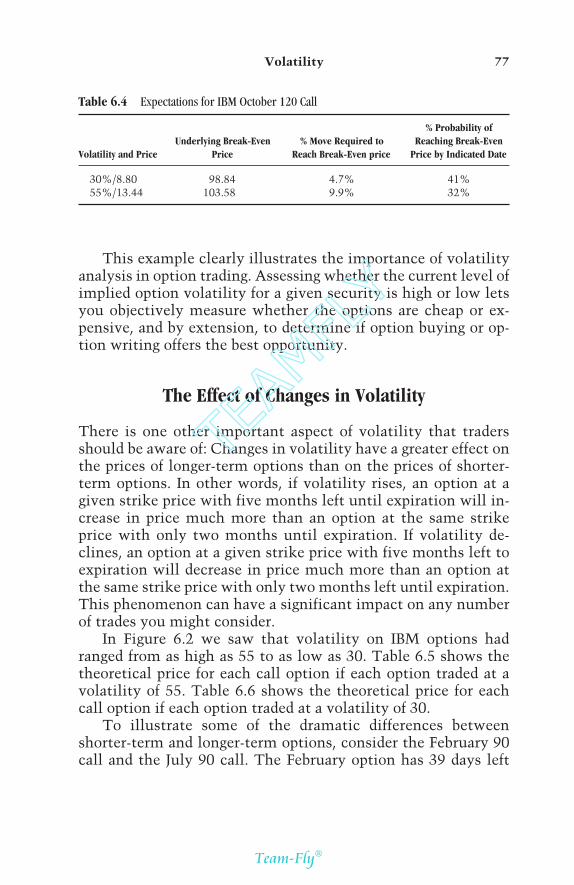
This example clearly illustrates the importance of volatilityanalysis in option trading. Assessing whether the current level ofimplied option volatility for a given security is high or low letsyou objectively measure whether the options are cheap or ex-pensive, and by extension, to determine if option buying or op-tion writing offers the best opportunity.
The Effect of Changes in Volatility
There is one other important aspect of volatility that tradersshould be aware of: Changes in volatility have a greater effect onthe prices of longer-term options than on the prices of shorter-term options. In other words, if volatility rises, an option at agiven strike price with five months left until expiration will in-crease in price much more than an option at the same strikeprice with only two months until expiration. If volatility de-clines, an option at a given strike price with five months left toexpiration will decrease in price much more than an option atthe same strike price with only two months left until expiration.This phenomenon can have a significant impact on any numberof trades you might consider.
In Figure 6.2 we saw that volatility on IBM options hadranged from as high as 55 to as low as 30. Table 6.5 shows thetheoretical price for each call option if each option traded at avolatility of 55. Table 6.6 shows the theoretical price for eachcall option if each option traded at a volatility of 30.
To illustrate some of the dramatic differences betweenshorter-term and longer-term options, consider the February 90call and the July 90 call. The February option has 39 days left
Volatility 77
Table 6.4 Expectations for IBM October 120 Call
% Probability of Underlying Break-Even % Move Required to Reaching Break-Even
Volatility and Price Price Reach Break-Even price Price by Indicated Date
30%/8.80 98.84 4.7% 41%55%/13.44 103.58 9.9% 32%
TEAMFLY
Team-Fly®

until expiration and the July option has 194 days. As you can seein Table 6.7, if volatility were to fall from 55 to 30—everythingelse being equal—the February 90 call would fall from a price of9.05 to 6.26, a loss of 2.79 points or –30.8%. At the same time,the July 90 call would fall from a price of 17.82 to 11.48, causinga loss of 6.34 points or –35.6%. Table 6.8 shows how manypoints each option would lose if volatility fell from 55 to 30.
78 The Option Trader’s Guide
Table 6.5 IBM Theoretical Option Prices for Implied Volatility of 55
Calls
JAN FEB APR JUL11 39 103 194
70 24.10 24.65 26.72 29.6375 19.13 20.10 22.85 26.2480 14.26 15.90 19.33 23.1585 9.74 12.19 16.19 20.3490 5.94 9.05 13.44 17.8295 3.18 6.50 11.06 15.57100 1.47 4.53 9.03 13.57105 .59 3.06 7.32 11.80110 .20 2.02 5.89 10.24115 .06 1.29 4.72 8.88120 .01 .81 3.76 7.69
Table 6.6 IBM Theoretical Option Prices for Implied Volatility of 30
Calls
JAN FEB APR JUL11 39 103 194
70 24.10 24.37 25.10 26.3875 19.11 19.42 20.43 22.0780 14.12 14.58 16.05 18.1185 9.17 10.07 12.14 14.5790 4.64 6.26 8.80 11.4895 1.56 3.44 6.12 8.88100 .30 1.66 4.08 6.75105 .03 .70 2.62 5.04110 .00 .26 1.62 3.70115 .00 .08 .96 2.68120 .00 .02 .55 1.92
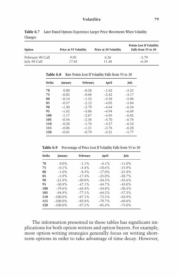
The information presented in these tables has significant im-plications for both option writers and option buyers. For example,most option-writing strategies generally focus on writing short-term options in order to take advantage of time decay. However,
Volatility 79
Table 6.7 Later-Dated Options Experience Larger Price Movements When VolatilityChanges
Points Lost If Volatility Option Price at 55 Volatility Price at 30 Volatility Falls from 55 to 30
February 90 Call 9.05 6.26 –2.79July 90 Call 17.82 11.48 –6.39
Table 6.8 Raw Points Lost If Volatility Falls from 55 to 30
Strike January February April July
70 0.00 –0.28 –1.62 –3.2575 –0.02 –0.68 –2.42 –4.1780 –0.14 –1.32 –3.28 –5.0485 –0.57 –2.12 –4.05 –5.8490 –1.30 –2.79 –4.64 –6.3495 –1.62 –3.06 –4.94 –6.69100 –1.17 –2.87 –4.95 –6.82105 –0.56 –2.36 –4.70 –6.76110 –0.20 –1.76 –4.27 –6.54115 –0.06 –1.21 –3.76 –6.20120 –0.01 –0.79 –3.21 –5.77
Table 6.9 Percentage of Price Lost If Volatility Falls from 55 to 30
Strike January February April July
70 0.0% –1.1% –6.1% –11.0%75 –0.1% –3.4% –10.6% –15.9%80 –1.0% –8.3% –17.0% –21.8%85 –5.9% –17.4% –25.0% –28.7%90 –21.9% –30.8% –34.5% –35.6%95 –50.9% –47.1% –44.7% –43.0%100 –79.6% –63.4% –54.8% –50.3%105 –94.9% –77.1% –64.2% –57.3%110 –100.0% –87.1% –72.5% –63.9%115 –100.0% –93.8% –79.7% –69.8%120 –100.0% –97.5% –85.4% –75.0%

if you are considering writing an option based primarily on an ex-pected decline in volatility, you may actually get more value foryour dollar by writing a longer-term option than a shorter-termone. Some traders buy long-term options so as to give themselvestime for their trades to work out. Unfortunately, if they do notpay attention to volatility and inadvertently buy long-term op-tions when volatility is high, they may sustain large losses ifvolatility falls, regardless of the action of the underlying security.
Summary
Option traders benefit from buying options when volatility islow because it means they are paying a lower price for the optionthan they would if volatility was high. This practice reduces theprice they pay for the option, which reduces their break-evenpoint and thus increases the probability of their earning a profit.By the same token, option writers benefit from writing optionswhen volatility is high because it means they take in more pre-mium, which in turn increases the probability that they willprofit. Changes in volatility after a particular trade is enteredcan also have a profound effect on the potential for profit.
Traders who buy or write options without any regard to thecurrent level of implied volatility or the effect that a significantchange in volatility might have on their positions are essentiallylike a sailors at sea without a compass.
80 The Option Trader’s Guide
Chapter 7
PROBABILITY
81
At its core, option trading is a game of odds. Therefore, those whohope to be successful at trading options must focus on consis-tently placing the odds as much in their favor as possible on atrade-by-trade basis. Assessing the probability of profit or loss ona potential trade or group of trades can be another key factor inoption-trading success. When you buy a stock (or go long a futurescontract), the results depend entirely on whether or not that secu-rity rises or falls in price after it is purchased. However, with mostoption trades the expectations are not as straightforward. Becauseoption prices include time premium—which will vanish by thetime of option expiration—from a strictly mathematical point ofview, an option buyer almost always has less than a 50% proba-bility of profit, whereas the option writer generally has a greaterthan 50% probability of profit. The tradeoff is that while buyers ofnaked options enjoy the prospect of unlimited profit potential andlimited risk, they also have a lower probability of profit. Con-versely, writers of naked options enjoy a higher probability ofprofit but assume limited profit potential and unlimited risk.
Weighing the Pros and Cons
Although anyone can form an opinion in each case, the fact is thatfor any given option trade there is no way to state definitivelywhether the option buyer or option writer has the upper hand.The key point is not to theorize about who has the edge, but to

• Compare the risk and reward characteristics of several possi-ble trades to determine which offers the most desirable trade-off between reward and risk.
• Simply be aware of the tradeoff being made. Too manytraders buy naked options, believing in the unlimited-profit,limited-risk mantra, without realizing that they are enteringinto low-probability trades. Doing so consistently can doomthem to failure. Other traders become enamored of theprospect of entering trades with a high probability of profit,which usually involves writing far-out-of-the-money options,without taking steps to minimize the attendant risk. Thistype of behavior is an invitation to disaster.
Even the casual option trader can benefit by learning to use prob-ability as an aid by simply adopting the habit of always buyingin-the-money options and writing out-of-the-money options. An-other useful technique is to analyze the risk curves for a varietyof possible trades in order to fully evaluate the relative risks andrewards associated with each position before making any trade.
Strategies for a Bullish Scenario
If a stock trader thinks a stock will advance in price, the choiceis simple: Buy the stock. For the option trader there are myriadchoices of potential trades. Each potential trade has its ownunique risk and reward characteristics. Let’s look at some exam-ples that illustrate this point. Consider a situation in which atrader wants to profit from an expected rise in the price ofa stock. We will consider three possible trading strategies tocompare their advantages and disadvantages.
These are the three strategies we will consider:
1. Buy 100 shares of stock at a price of $94 a share.2. Buy 1 February 90 call option at 9.88.3. Write 10 February 75 put options at 1.375.
Figures 7.1 through 7.3 depict the expected profit or loss foreach position through a range of prices from 64 to 124.
82 The Option Trader’s Guide

Buying 100 Shares of Stock at 94
To purchase these shares traders must put up $9400 ($94 × 100shares). One advantage of this position is that the traders actuallyown a piece of the company. They can hold the stock for as shortor as long a time as they want. If they believe that the company
Probability 83
3000
2000
1000
0
–1000
–2000
–300064.00 74.00 84.00 94.00 104.00 114.00 124.00
Date: 4/20/01 Profit/Loss: –1 Underlying: 94.07 Above: 49% Below: 51% % Move Required: +0.6%
Figure 7.1 Risk curve for buying long 100 shares of IBM at 94.
2403
1802
1202
601
0
–601
–120264.00 74.00 84.00 94.00 104.00 114.00 124.00
Date: 2/16/01 Profit/Loss: –9 Underlying: 99.85 Above: 35% Below: 65% % Move Required: +5.8%
Figure 7.2 Risk curve for buying 1 February 90 call at 9.88.

has brilliant long-term prospects, they can simply hold the stockand wait to enjoy the hoped-for benefits. Compared to the otherchoices in this example, the biggest advantage of this position isthat traders are guaranteed point-for-point movement if the stockprice goes up. The primary disadvantage of this position is the riskof suffering a point-for-point loss if the stock declines in price.
Buying 1 February 90 Call Option at 9.88
To purchase one February 90 call option traders must invest only$988, compared to the stock buyers, who must invest $9400.The biggest advantage of this position is that although tradersput up only about one-tenth as much as buyers of 100 shares ofstock, they still enjoy the possibility of point-for-point move-ment with the stock above a price of 98.88. If the stock risesstrongly, they would enjoy a greater percentage rate of returnthan would stock buyers. On the downside, they would lose$988, or 100% of the investment, if IBM closes at 90 or lower atthe time of option expiration. Nevertheless, unlike stock traders,who lose more money for every point the stock declines, theycan lose no more than the $988 they put up to enter the trade, re-gardless of how far the stock may decline.
84 The Option Trader’s Guide
1605
–268
–2140
–4012
–5885
–7758
–963064.00 74.00 84.00 94.00 104.00 114.00 124.00
Date: 2/16/01 Profit/Loss: –11 Underlying: 73.71 Above: 95% Below: 5% % Move Required: –21.4%
Figure 7.3 Risk curve for writing 10 February 75 puts at 1.375.
Writing 10 February 75 Put Options at 1.375
Writing put options is by far the most exotic of the three strate-gies. When buying stock or buying an option, traders put up thefull amount of the purchase price in cash in order to enter thetrade. When writing a naked option (which is the same as sellingshort an option), traders are required to put up margin. Margin isa good-faith deposit intended to guarantee that traders will meettheir obligations if the option they have written is exercisedagainst them. For naked options written on stocks, the formulafor calculating margin requirements is 20% of the price ofthe stock minus the amount by which the option is out of themoney. If this value is less than 10% of the price of the stock(times $100), traders must put up a minimum of 10% of the priceof the stock (times $100).
The amount of margin required can fluctuate as the price ofthe stock rises or falls. If the stock begins to fall, naked optionwriters may be required to add more margin money to covertheir margin requirement. Ultimately, writers of the naked putmay be required to buy 100 shares of stock at the strike price foreach option they have written. In the worst-case scenario for thistrade, the writers would have to buy 100 shares of stock at $75 ashare for each option contract assigned to them.
For this example, using the original margin requirement for-mula would result in a negative margin requirement, so the 10%rule applies. In other words, with IBM trading at 94, traders mustput up $940 for every February 75 put option they want to write.Thus, to write 10 February 75 put options, traders must put up$9400 in margin money.
Original formula (stock price × 20%) – (strike price – stock price)
((94 × .20) – (75 – 94) × 100)((18.8 – 19) × 100) = –20
Minimum margin (stock price × 10%) × 100(94 × 0.1) × 100 = $940
Margin on 10 contracts $940 × 10 = $9400
The biggest advantage to this position is that traders can earna profit even if the stock price falls significantly. The break-even
Probability 85

price for this trade is 73.62 (equal to the strike price of 75 minusthe premium collected of 1.375). In other words, if IBM stockfalls to 75 at the time of February option expiration, the tradersstill get to keep the entire $1375 they collected when they wrotethe options. Also, based on the historic volatility for IBM atthe time of this trade, there is a 95% probability that IBM will beabove the break-even price of 73.62 at the time of expiration.This high probability of profit is what draws many traders towriting options. Nevertheless, there are several negatives asso-ciated with writing naked options that must be carefullyweighed before employing this strategy.
First, although the initial margin requirement to write oneoption ($940) is relatively low, the amount of margin money re-quired would increase if the price of the stock began to fall. Forexample, if the stock fell to 80, the margin requirement for thisposition would rise to $1100 per contract. Also, should the priceof the stock ultimately fall below 75, the traders would have toconsider buying back the options—quite possibly at a signifi-cantly higher price—or the options may be exercised againstthem. If the options are exercised against the traders, the optionwriters are obligated to buy the 100 shares of stock at $75 ashare. In other words, they would need $7500 per contract. Awriter who is assigned on 10 option contracts would be requiredto buy $75,000 worth of stock (see Chapter 17 for a complete dis-cussion of the strategy of writing naked puts). This representsa far different commitment than the initial margin requirementof $9400.
Profit/Loss Comparisons
Figures 7.1, and 7.2, and 7.3 depict the relative expectations as-sociated with each of the three potential trades. Note that eachof these trades will indeed make money if the stock rises. Thevariables are
• The amount of money required to enter each trade• The dollar and percentage amount of profit to be obtained
with each trade• The worst-case scenario for each trade
86 The Option Trader’s Guide

Tables 7.1 and 7.2 depict the various entry considerationsand expected returns over a range of stock prices for these threepositions. If you were to ask 100 traders which of these three op-portunities qualifies as the best trade, you would get a number oftraders in each camp. The problem in this case—and with everynew trade you consider—is not which is the best trade to make.
Probability 87
3000
2000
1000
0
–1000
–2000
–300064.00 74.00 84.00 94.00 104.00 114.00 124.00
Date: 4/20/01 Profit/Loss: –1 Underlying: 94.07 Above: 49% Below: 51% % Move Required: +0.6%
Figure 7.1 Risk curve for long buying 100 shares of IBM at 94.
2403
1802
1202
601
0
–601
–120264.00 74.00 84.00 94.00 104.00 114.00 124.00
Date: 2/16/01 Profit/Loss: –9 Underlying: 99.85 Above: 35% Below: 65% % Move Required: +5.8%
Figure 7.2 Risk curve for buying 1 February 90 call at 9.88.
TEAMFLY
Team-Fly®

88 The Option Trader’s Guide
Table 7.1 Break-Even Analysis (Current Stock Price = 94)
Probability of Initial Stock Break-Even Percentage Move Reaching
Trade Entered Cost Price Required Break-Even
Buy 100 shares $9400 94 0% 50%at $94
Buy 1 February 90 $988 98.88 +5.8% 35%call at 9.88
Write 10 February $9400* 73.62 Anything better 95%75 puts at 1.375 than a decline of
–21.4% or more
*Required margin may vary as stock price changes.
Table 7.2 Expected Returns Depending on Stock Price Movement
Trade Stock Down Stock Down Stock Stock Up Stock Up Entered 30 Points 15 Points Unchanged 15 Points 30 Points
Buy 100 shares –$3000 –$1500 $0 +$1500 +$3000 at $94 (–32%) (–16%) 0% +16% +32%
Buy 1 February –$988 –$988 –$488 +$913 +$2513 90 call at 9.88 (–100%) (–100%) (–49%) +92% +154%
Write 10 February –$11000 +$1375 +$1375 +$1375 +$1375 75 puts at 1.375 (NA) +15% +15% +15% +15%
1605
–268
–2140
–4012
–5885
–7758
–963064.00 74.00 84.00 94.00 104.00 114.00 124.00
Date: 2/16/01 Profit/Loss: –11 Underlying: 73.71 Above: 95% Below: 5% % Move Required: –21.4%
Figure 7.3 Risk curve for writing 10 February 75 puts at 1.37.

The question that a trader needs to answer is “Which trade bestfits my expectations and my risk tolerance constraints?” It is im-possible to overstate the importance of giving yourself an honestanswer each time out.
Delta
A value referred to as an option’s delta can be calculated for eachoption by an option-pricing model. The delta value can rangefrom 0 to 100 for calls and from 0 to –100 for puts. The signifi-cance of a particular option’s delta value can be viewed in threeways:
1. The delta value for a given option provides an estimate of theprobability that the option will expire in the money. Thus,an option with a delta of 20 currently has a roughly 20%probability of expiring in the money (although this is notmathematically correct, it does provide a useful estimate anda valuable frame of reference). This aspect of delta can be es-pecially useful in assessing the probability of profit whencomparing possible trades.
2. A delta value of 25 implies that if the underlying stock in-creases one full point, the option will increase in value by0.25 point.
3. A delta value of 100 indicates that the option position is cur-rently the equivalent of holding 100 shares of stock (or beinglong one futures contract). Thus, buying a put option with adelta of –40 means the position is presently equivalent tobeing short 40 shares of the underlying stock (or being shortfour-tenths of one futures contract). You should be awarethat this is not a static value. The delta value for an optionwill change as time passes and as the underlying security’sprice rises or falls.
Table 7.3 displays the delta values for a series of call and putoptions for IBM on January 5 with the stock trading at $94. Thefurther in the money a call option is, the higher its delta value.The further out of the money a call option is, the lower its deltavalue. This makes intuitive sense when you consider that the
Probability 89
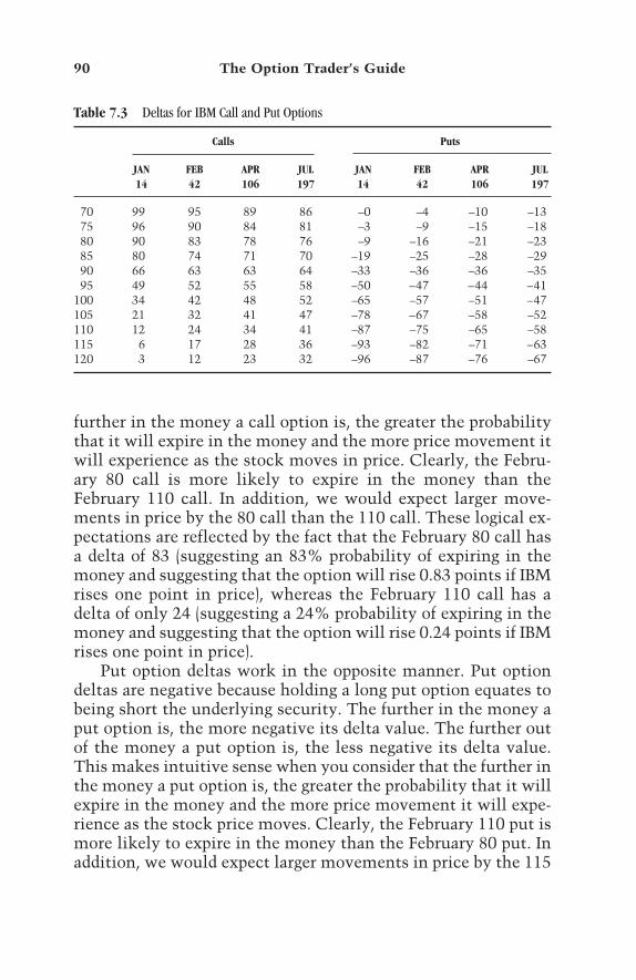
further in the money a call option is, the greater the probabilitythat it will expire in the money and the more price movement itwill experience as the stock moves in price. Clearly, the Febru-ary 80 call is more likely to expire in the money than theFebruary 110 call. In addition, we would expect larger move-ments in price by the 80 call than the 110 call. These logical ex-pectations are reflected by the fact that the February 80 call hasa delta of 83 (suggesting an 83% probability of expiring in themoney and suggesting that the option will rise 0.83 points if IBMrises one point in price), whereas the February 110 call has adelta of only 24 (suggesting a 24% probability of expiring in themoney and suggesting that the option will rise 0.24 points if IBMrises one point in price).
Put option deltas work in the opposite manner. Put optiondeltas are negative because holding a long put option equates tobeing short the underlying security. The further in the money aput option is, the more negative its delta value. The further outof the money a put option is, the less negative its delta value.This makes intuitive sense when you consider that the further inthe money a put option is, the greater the probability that it willexpire in the money and the more price movement it will expe-rience as the stock price moves. Clearly, the February 110 put ismore likely to expire in the money than the February 80 put. Inaddition, we would expect larger movements in price by the 115
90 The Option Trader’s Guide
Table 7.3 Deltas for IBM Call and Put Options
Calls Puts
JAN FEB APR JUL JAN FEB APR JUL14 42 106 197 14 42 106 197
70 99 95 89 86 –0 –4 –10 –1375 96 90 84 81 –3 –9 –15 –1880 90 83 78 76 –9 –16 –21 –2385 80 74 71 70 –19 –25 –28 –2990 66 63 63 64 –33 –36 –36 –3595 49 52 55 58 –50 –47 –44 –41
100 34 42 48 52 –65 –57 –51 –47105 21 32 41 47 –78 –67 –58 –52110 12 24 34 41 –87 –75 –65 –58115 6 17 28 36 –93 –82 –71 –63120 3 12 23 32 –96 –87 –76 –67

put than the 80 put. These logical expectations are reflected bythe fact that the February 110 put has a delta of –75 (suggestinga 75% probability of expiring in the money and suggesting thatthe option will rise 0.75 points if IBM falls one point in price),whereas the February 80 call has a delta of only –16 (suggestinga 16% probability of expiring in the money and suggesting thatthe option will rise 0.16 points if IBM falls one point in price).
Traders often attempt to position trades so that they aredelta neutral. This simply means putting on a combination ofoption positions so that when the positive and negative deltasare added together, the net result is as close to zero as possible.As long as a position is delta neutral, the price movement of theunderlying security doesn’t matter. Nevertheless, traders shouldbe aware that option deltas change as the underlying marketprice moves. Thus, a trade that is delta neutral today may not bedelta neutral tomorrow and may require a trader to either closethe position, or rebalance the net position by closing out somepositions or opening others to achieve delta neutrality onceagain.
Probability Analysis
It is possible to estimate the probability of profit for any givenoption trade by considering the volatility in price movementthat a stock or futures contract has exhibited in the past. This in-formation can be extremely useful when attempting to choosebetween more than one potential trade. For each option tradeyou can determine, or at least approximate, the break-evenpoint. Using the historical volatility of the underlying security,you can then calculate the probability that the break-even pricewill be reached by some target date in the future. Let’s look at anexample to illustrate this concept.
Suppose a trader wanted to buy a straddle on Microsoft onJanuary 5 with Microsoft trading at 49.12. For a trader willing tocommit $3500 to a trade, here are two possibilities:
1. February 50 straddleBuy 4 February 50 calls at 4.25Buy 4 February 50 puts at 4.50
Probability 91

2. February 55/45 straddleBuy 7 February 55 calls at 2.31Buy 7 February 45 puts at 2.62
The risk curves for these two trades are shown in Figures 7.4 and7.5. The key question for a trader is “Which trade should Imake?” There are several factors to assess before an informed de-
92 The Option Trader’s Guide
4850
1886
–1078
–404229.13 35.81 42.44 49.13 55.81 62.44 69.13
Figure 7.4 Risk curves for Microsoft 50 call/50 put straddle.
7661
5746
3831
1915
0
–1915
–383129.13 35.81 42.44 49.13 55.81 62.44 69.13
Figure 7.5 Risk curves for Microsoft 55 call/45 put straddle.

Probability 93
Probability Analysis
Current Date 1/5/01 Current Price 49.12Future Date 2/16/01 Upper Target: 59.09Number of Days 42 Prob. Reach: 11.03%Current Price 49.12 Prob. Not Reach: 88.97%Volatility 44.49 Lower Target: 41.04Upper Price Target 59.09 Prob. Reach: 11.68%Lower Price Target 41.04 Prob. Not Reach: 88.32%
Prob. of Closing between Targets: 77.29%
Figure 7.6 Probability of exceeding break-even prices at expiration for the Microsoft 50straddle.
cision can be made; probability analysis can help in several areas.Consider the following:
• The distance between the current underlying price and thebreak-even points and the probability of closing outside thesebreak-even points
• The expected return if the underlying stock makes a bigmove and the probability of actually achieving a big move
• The worst-case scenario and the probability of experiencingit
Figure 7.6 displays an analysis of probability for the 50 strad-dle. These are the key points:
• The 50 call/50 put spread costs $3500 to enter.• The break-even points for this trade are 59.09 on the upside
and 41.04 on the downside.• With the stock at 49.12 and a historical volatility of 44.49,
the probability of closing outside these break-even points atexpiration is 22.71% (100% – 77.29%).
• A move of two standard deviations between January 5 andFebruary option expiration would reach 63.89 on the upsideor 34.36 on the downside.
• At 63.89 this trade would show a profit of $2056. At 34.36this trade would show a profit of $2755.

Figure 7.7 shows an analysis of probability for the 55/45straddle. These are the key points:
• The 55 call/45 put spread costs $3456 to enter.• The break-even points for this trade are 60.08 on the upside
and 39.81 on the downside.• With the stock at 49.12 and a volatility of 44.49, the proba-
bility of closing outside these break-even points at expirationis 17.28% (100% – 82.72%) (see Figure 7.7).
• A two-standard deviation move between January 5 and Feb-ruary option expiration would reach 63.89 on the upside or34.36 on the downside.
• At 63.89 this trade would show a profit of $2772. At 34.36this trade would show a profit of $3996 (see Figure 7.7 andTable 7.4).
Table 7.4 illustrates the tradeoffs that must be consideredwhen selecting trades to make—and it shows why there is a highrate of failure among option traders in general. It can be arguedthat traders should never consider entering a straddle unless theyare highly confident that the underlying security will make a bigmove. In this example, if you truly expect Microsoft to make abig move in price, you should presumably buy the 55 call/45 putstraddle, since that trade has the greatest profit potential. Butconsider the tradeoffs:
94 The Option Trader’s Guide
Probability Analysis
Current Date 1/5/01 Current Price 49.12Future Date 2/16/01 Upper Target: 60.08Number of Days 42 Prob. Reach: 9.10%Current Price 49.12 Prob. Not Reach: 90.90%Volatility 44.49 Lower Target: 39.81Upper Price Target 60.08 Prob. Reach: 8.18%Lower Price Target 39.81 Prob. Not Reach: 91.82%
Prob. of Closing between Targets: 82.72%
Figure 7.7 Probability of exceeding break-even prices for the Microsoft 55/45 straddle atexpiration.

• The break-even points for the 55/45 straddle are further awaythan the break-even points for the 50 straddle, thus the 55/45trade has a lower probability of profit.
• There is a far higher probability of sustaining a 100% losswhile holding the 55/45 straddle until expiration than thereis for the 50 straddle. The 50 straddle will sustain a 100%loss only if Microsoft is trading at exactly 50 at the time ofFebruary expiration. The 55/45 straddle will sustain a 100%loss if Microsoft is trading anywhere from 45 to 55 at thetime of February expiration. At any price between 45 and 55,the 55/45 straddle will lose more money than the 50 straddle.
In sum, if a trader is going to trade straddles only occasion-ally, when he or she is highly confident that a big move is im-minent, then a trade similar to the 55/45 straddle in thisexample makes sense because it offers the greatest potential re-turn. Conversely, any trader who is planning to trade straddleson a regular basis might be better off using something like the 50straddle in this example in order to minimize losses when theunderlying security does not move as expected.
The Correct and Incorrect Ways to Use Probability
The primary mistakes traders make in assessing probability are
Probability 95
Table 7.4 Summary of Primary Considerations
Consideration 50 Straddle 55 Call/45 Put Straddle
Upside break-even point 59.04 60.08Downside break-even point 41.04 39.81Probability of being outside break-even 22.7% 17.3%
points at expiration2-standard-deviation up target 63.89 63.892-standard-deviation down target 34.36 34.36Profit at 63.89 at expiration $2056 $2772Profit at 34.36 at expiration $2755 $3996Straddle experiences maximum loss if stock 50 45 to 55
is between values at rightProbability of experiencing maximum loss Less than 1% 49.2%

• Failing to assess the likelihood of making money before en-tering into a prospective trade
• Failing to manage their trades properly after they enter intothem because they assume that the probabilities are on theirside
Though it is hard to believe, it is a fact that most optiontraders have no idea what the probability is of making money ona particular trade when they enter into it. Consider that if youbuy a call option with a delta of 33, you have only about a 1:3chance of breaking even if you hold the option until expiration(this fact alone goes a long way toward explaining why specula-tors who only buy cheap, out-of-the-money options generallylose money in the long run).
On the other end of the spectrum, a trader may write a far-out-of-the-money call option with a delta of 10, realizing thatthis implies a 90% probability of making money (i.e., the optionwill expire out of the money and thus become worthless). This isa useful method for selecting options to write. The paradox,however, is that once this trade is entered, the proper question isno longer “What was my probability of making money when Ientered the trade?” but “What am I going to do if the marketmoves sharply against me and I am faced with a loss?” If the un-derlying market rallies sharply, the trader in this example mustact to cut losses, regardless of the initial probability of profit.
Following are the key points to remember about deltas andprobability:
• You should assess the probability of profit before entering atrade.
• Do not put too much faith in the initial probability of profitonce a trade is made. The probability of profit calculatedwhen you enter a trade means nothing once you actuallyenter the trade. Once a trade is entered, it must be managedon the basis of dollars and cents, not probability.
Summary
For any given option trade it is possible to estimate the proba-
96 The Option Trader’s Guide
bility of profit or loss. An estimate is nothing more than an ap-proximation, but this information can be extremely useful inhelping a trader to choose between several potential trades. Itcan also be useful in assessing the trade off between reward andrisk for any given trade.
As a simple tool, an option’s delta value serves as a handy es-timate of the likelihood that it will expire in the money. This in-formation alone can often help astute traders to zero in on thespecific option or options most likely to help them achieve theirobjectives. The historic volatility of the underlying security alsocan be used to estimate the likelihood that a given option tradewill reach its breakeven point before option expiration. Informa-tion is power. Recognizing the likelihood of your success in ad-vance is an area of analysis that far too many traders overlook.
Probability 97
TEAMFLY
Team-Fly®


Chapter 8
MARKET TIMING
99
As we have seen in previous chapters, many elements play im-portant roles in your success or failure as an option trader. An-other important factor is market timing. Depending on the typeof option trading you do, timing can play a crucial role in yoursuccess. When you buy a stock or a futures contract, your timingmust be reasonably good for you to make money. In other words,the price of the stock or futures contract must rise from its cur-rent level without first falling so far in price that you feel youmust sell to cut your loss.
Probability, volatility, time until expiration, and volatilityskew are important factors in the success or failure of trade, butthe value of some strategies hinges primarily on accurate timing.Market timing has been the subject of thousands of books, arti-cles, and videotapes. An exhaustive discussion of market timingis beyond the scope of this discussion, but we can touch on sev-eral option-trading situations in which timing plays a criticalrole. Some examples of each situation are provided to help youfocus your attention in the right areas. These situations includethe following:
• The underlying stock or futures contract is expected to movein a particular direction within a specific period.
• The underlying stock or futures contract is expected to trendin a particular direction without a specific time frame.
• The underlying stock or futures contract is expected to movesignificantly, but the direction is unknown.

• The underlying stock or futures contract is expected to stayin a particular range or at least not to move very far in anydirection.
Options can be used to maximize your profitability given anyof the preceding expectations. Two keys are
1. Being correct about your expectations2. Using the proper trading strategy given your expecta-
tions and the current volatility level for the options on theunderlying
Key 1 generally determines whether or not you will make moneyon your trade. Key 2 determines how much money you canmake.
The Underlying Security Is Expected to Movewithin a Specific Period
If you are planning to buy naked calls and puts, it is crucial thatyou use a successful timing technique. If you buy calls and theunderlying security falls in price or if you buy puts and the un-derlying security rises in price, you will invariably lose money.For traders who develop their own trading systems, one of thebest tests you can run on a system for the purpose of buyingnaked calls and puts is to develop entry criteria and measure theprice movement some number of days (x) later (testing differentday windows as the variable x).
In other words, if you develop an entry criterion for buyingcalls and find that 70% of the time the underlying security ishigher 5 days later, you have a very powerful tool for trading op-tions. The criterion can be almost anything and the time framecan vary from one day to many months. With options, there arecertain potential advantages associated with targeting a specifictime frame.
The primary advantage of using a specific time frame is thatit allows you to focus on a single strategy with certain expecta-tions and without as much concern for factors you might other-
100 The Option Trader’s Guide

wise have to consider. Let’s look at an example. If you adopt astrategy that targets a 5-day time frame, such as buying a call op-tion with the expectation of selling it within 5 trading days, youdo not have the same concerns about changes in volatility andtime decay as the trader who buys a call expecting a longer-termtrend to develop.
If you are going to buy a naked call option with the idea ofholding it for a month or more, you need to be very concernedwith the level of implied volatility for that security when youenter the trade (see Chapter 6). If volatility is extremely high,you pay a lot more time premium than if volatility were low.Hence, you must be concerned about a decline in volatility,since such a decline would lower the price of all options on thatsecurity, including yours. In addition, you must be concernedabout time decay since all the time premium you paid will decayas option expiration draws nearer.
If you buy an option with the intention of selling it within 5days, you do not need to be quite as concerned about volatilityand time decay. Certainly it is possible for volatility to fall sig-nificantly in a short period, but it is less likely to do so in thenext 5 days than it is in the next month or more. Also, if youtrade with a 5-day time frame, and as long as you don’t buy op-tions with less than a few weeks until expiration, you don’t needto concern yourself as much with time decay. Although timepremium on every option decays at least a small amount eachday (see Chapter 5), the biggest effect is seen in the last fewweeks before expiration.
On the other hand, the glaring disadvantage to trading with aparticular time frame in mind is that the underlying securitymust make a move within your time frame or you will losemoney. You also lose the opportunity to participate in majorlong-term trends.
Figure 8.1 depicts trading signals on the S&P 100 (OEX) stockindex. (All figures in this chapter appear courtesy of Option Pro,Essex Trading Co., Ltd.) This system uses a moving average todetermine the trend and then uses Welles Wilder’s relativestrength indicator to identify pullbacks against that trend inorder to identify an entry signal. Finally, the trade is exited aftereither 7 trading days or an overbought reading (if holding calls) or
Market Timing 101

an oversold reading (if holding puts) from another momentumoscillator.
The Underlying Is Expected to Move in a ParticularDirection but Not in a Specific Time Frame
Traders often decide that they expect a security to rise or fall, butthey have no specific time frame in mind. Here, too, options canbe used to maximize profitability, but other concerns specific tooption trading must be taken into consideration.
Figure 8.2 depicts trading signals for Intel from a trend-following system. The system generates a buy-calls or buy-putssignal and holds that position indefinitely, depending on the ac-tion of the stock. As a result, a trade could conceivably last a day,a week, a month, or longer. However, there is no way to know atthe time of the initial entry signal how long the trade will last.This has important implications for an option trader.
Option traders using a trend-following method such as thisabsolutely must take steps to minimize the amount of time
102 The Option Trader’s Guide
83132
81332
79532
77732
75932
74132
72332330 424 516 609 705 727 821
Calls were purchased.Calls were sold.
Buy calls Buy puts Exit tradeor
Figure 8.1 Example of short-term trading signals on the S&P 100 (OEX).

decay their trades are exposed to. A trader trading without aspecific time frame, who routinely buys expensive (i.e., high-volatility) options, will invariably lose money in the long runbecause time decay or declines in volatility, or both, will even-tually eat away too much of the profit potential.
The Underlying Is Expected to Move Significantly butthe Direction Is Unknown
One opportunity that is unique to option trading is the ability toenter a position that will create a profit whether the price of theunderlying security rises or falls. The most common approach isto buy a straddle (see Chapter 15), which involves buying a calloption and a put option simultaneously. The only reason to usethis strategy is if you expect the underlying security to make alarge price move and are not sure which direction it will move.
In general, stocks and futures markets tend to trend for awhile and then consolidate for a while, then trend again, and so
Market Timing 103
7577
6811
6045
5279
4513
3747
2981612 718 822 929 1106 1212 10119
Buy calls Buy puts Profit-taking opportunityor Exit trade
Figure 8.2 Trend-following trading signals on Intel.

on. If you can identify a security that has been consolidating fora long time, you may surmise that it is likely to begin a newtrend soon. If the only vehicle you have at your disposal is buy-ing or selling short that stock or futures market, you mustchoose the direction you expect the anticipated trend to go. Ifyou choose the right direction, you stand to make money; if youchoose the wrong direction, you stand to lose money. In essence,you have a 50:50 chance of being right. Alternatively, instead ofpicking a direction, you can buy a call and a put simultaneouslyand wait for the underlying security to show a trend.
Figure 8.3 shows a proprietary oscillator that attempts to dis-cern when a security is likely to trend, without giving any indi-cation as to the direction of that trend. Whenever this oscillatorexceeds 90 on the upside or 10 on the downside, it is suggestingthat a trend may soon develop. Each such reading is marked onthe chart by an up arrow and a down arrow. There are seven suchsignals on this chart for the underlying stock, America Online(AOL). Six of the seven signals were followed by price move-ments large enough to yield a profit to a trader who had boughta call and a put at the time of each signal.
104 The Option Trader’s Guide
9598
8359
7120
5881
4642
3403
2164990127 990326 990527 990729 990928 991126 128
Buy calls and put
Figure 8.3 Nondirectional signals on America Online.

Traders can use a number of measures to identify quiet mar-kets. Although a thorough discussion of the indicators is beyondthe scope of this book, some examples that industrious tradersmay wish to explore are ADX, historical volatility ratios (e.g.,the 6-day historical volatility divided by the 100-day historicalvolatility), and the number of trading days since the last x-dayhigh or low.
The Underlying Is Expected to Stay within a Range orNot Move Much in Any Direction
One more opportunity unique to option trading is the potentialto make money when a security does nothing. As discussed else-where in the book, there are a number of ways to take advantageof neutral situations, when a security displays no trend at all.Entry timing for these types of trades can be triggered by certainindicators, or more subjectively, by observing on a bar chart thata given security is presently bracketed by significant support andresistance levels.
Figure 8.4 shows several signals for Conseco (CNC) based onWelles Wilder’s the ADX Directional Movement Index (DMI) in-dicator (on a scale of 0 to 100) exceeding the 75 level on the up-side. These signals often indicate an overbought security thatmay be due for some consolidation. Overbought readings arenoted by a solid down arrow. The overbought situation takesprecedence over the ADX DMI indicator dropping below 50,which is shown by an empty down arrow.
Identifying overbought situations can be a very useful timingtechnique for investors who write covered calls. As you can seein Figure 8.4, between each solid arrow and each empty arrowthe stock traded sideways to lower. A holder of Conseco stockcould potentially have written out-of-the-money calls and col-lected premium as the stock trended lower.
Other strategies can be used to exploit this going-nowheresituation. They include buying calendar spreads, selling verticalspreads, selling naked puts, and entering butterfly spreads (seeChapters 14, 16, 17, and 19).
Market Timing 105

Summary
Market timing is essentially a quest for the holy grail. Some-times a trader’s timing is good, and sometimes it is not. Accuratetiming when entering and exiting option trades can greatly in-crease your trading profits, and poor timing can generate largelosses over time. The purpose of this chapter is not to reveal anymystical secrets of market timing but to start option tradersthinking in terms of time frame and situation. Entirely differenttiming methods may be appropriate for a trader who is attempt-ing to take advantage of a short-term move than for one who istrying to capture a long-term trend.
106 The Option Trader’s Guide
1172
1060
948
836
724
612
500613 713 811 913 1016 1115 1218
Overbought stock.ADX DMI < 50.
Figure 8.4 Covered call-writing opportunities for Conseco.

Chapter 9
TRADING REALITIES
107
Theory is one thing, reality is another. Nowhere is this truerthan in the world of trading. At times it seems that there is achasm a mile wide between theory and reality. In the real worldof trading, all our well-thought-out trading plans, time-tested in-dicators, reliable patterns, and well-established relationships cansuddenly stop working—completely and permanently—leaving apractitioner of these methods in danger of losing significantmoney. In a slightly less dire vein, often the simple day-to-daymechanics of trading can be different from what a trader ex-pected them to be. This too can act as a serious impediment tolong-term success. For example, if your method requires spend-ing an hour a day updating data, analyzing markets, and placingorders, but you have only 30 minutes a day to devote to thesetasks, then your approach has a fatal flaw that will likely costyou a lot of money.
This chapter discusses some realities of option trading thatyou should give some serious thought to. These can seem fairlymundane, but they can make a major difference in your trading.
Exercise and Assignment
If a call holder decides she wants to buy the underlying stock, orif a put holder decides he wants to sell the underlying stock,each would exercise his or her option. To do this, the buyer ofan option indicates to her broker that she wants to exercise her
TEAMFLY
Team-Fly®

option. Using something like a lottery process, some trader whois short that particular option would be assigned the obligationto deliver 100 shares of stock to the call option buyer. For exam-ple, say a trader is long one March call option with a strike priceof 55. The stock rises to 65 and the trader decides she wants toown the stock. To make this happen she would call her brokerand say that she wants to exercise this particular option. A traderwho previously sold short the March 55 call and had not yetbought it back would be assigned on the option. This traderwould need to either buy 100 shares of stock in the open marketand deliver them to the option buyer (at a price of $55 per share)or deliver 100 shares of stock he already holds.
On the put side, consider a trader who is long one March putoption with a strike price of 55. The stock falls to 45 and thetrader decides he wants to short the stock from 55. To make thishappen he calls his broker and says that he wants to exercisethis particular option. A trader who previously sold short theMarch 55 put and has not yet bought it back would be assignedon the option. This trader would need to sell short 100 shares ofstock in the open market and deliver them to the option buyer(for a price of $55 a share) or deliver 100 shares of stock she al-ready holds short.
Another consideration often overlooked by novice traders isautomatic exercise. When stock and stock index options expire,the Option Clearing Corporation automatically exercises anyunclosed long call or put position that is at least one-eighth of apoint in the money at the time of expiration. Because of this, inmost cases, traders who are short an in-the-money option nearexpiration are best advised to close that position before expira-tion, unless they specifically want to hold a position, be it longor short, in the underlying security. Many a novice trader hasbeen surprised on Monday morning after expiration to be holdinga long or short position in the underlying.
Options can be either American style or European style.American style options can be exercised at any time up until op-tion expiration. European style options can only be exercised atexpiration. Most U.S. stock options are American style, andmany stock index options are European style.
108 The Option Trader’s Guide

The Implications of Exercise
Though it does not get talked about much, the unexpected ex-ercise of a short option position can have significant implica-tions. Myriad spread strategies are available to an option trader.Some involve buying options at one strike price and selling op-tions at another strike price. Traders often put on such tradesafter inspecting a risk curve that shows the expected profit orloss at expiration, thinking they will simply close out the tradeat expiration with the indicated profit or loss. However, if the op-tion (or options) they sold short as part of a spread were to tradedeep in the money before expiration, there is a very real likeli-hood that the trades will be assigned on that option, forcingthem to deliver stock while still holding the other options intheir spread. This event can throw the expected results way outof whack.
Getting assigned on a short option is not a catastrophic eventin and of itself. The important point is that the writer of an op-tion must be aware of the possibility of getting assigned on thatoption and the potential impact of this event on the intendedstrategy.
When to Expect an Option to Be Exercised
There are two primary situations in which a trader can expect anoption to be exercised. The first situation is at expiration. If youare holding a long option that does not settle in cash and youhold the position through expiration, you will end up with a longposition in the underlying security. If you are short an optionthat does not settle in cash and you hold the position through ex-piration, you will end up with a short position in the underlyingsecurity.
You should also be concerned about being exercised on ashort option if it is trading deep in the money. As a rule ofthumb, if an option is trading at parity (i.e., there is no time pre-mium in the price of the option) or just slightly above parity, youcan generally expect it to be exercised.
Trading Realities 109

An Example
One popular strategy for which option exercise is relevant is abackspread. Chapter 13 presents the various considerations forusing a backspread. For now we focus solely on how early exer-cise can affect this trade. As an example of a backspread considera position in which a trader sells one 50 call option at a price of5 points and buys two 55 call options at a price of 2 points each.If the underlying stock rallies up to 70 or higher, the 50 call op-tion that was written will be deep in the money. Once it loses al-most all its time premium, the odds are great that the option willbe exercised. Should this happen, the trader will have to eitherbuy 100 shares of the underlying stock to deliver or buy back theoption he has written. In either case he leaves himself with twolong calls, which is not a position he intended to be in. If thestock price then falls, he stands to take serious losses as the longcalls decline in price and he no longer has the short call positionto offset some or all of those losses. His other alternative is to ex-ercise one of his long calls. Should he choose this route, hewould then be left with one long call option, which again isnot the position he intended to be in when he entered into abackspread.
The question is not whether the trader in this example willultimately make or lose money on this trade. The point of thisexample is to illustrate how the position he ended up with wasfar different from the one he intended to be in when he enteredthe trade. In the end he may make money, but not without firsthaving to make some quick and unexpected decisions. What isimportant to understand is that the possibility for this type ofsituation exists whenever an option that you have written tradesdeep in the money.
Bid and Ask Prices and the Importance of Option Volume
When the time comes for new traders to move past the learningstage, after they have spent a lot of time absorbing the theory ofoptions, the next step is to begin placing real orders, making real
110 The Option Trader’s Guide

trades, and getting real fills. At this point many new traders ex-perience something of a shock. When new traders test out theirtrading strategies, they often pull option prices out of the news-paper and assume that the price that appears in the newspaperwas the price at which they bought or sold. In fact, many newtraders make the mistaken assumption that if a price is printedin the paper they can buy or sell as many options as they want toat that price. This is not true.
When you place an order to buy (or sell) a given option, youcan obtain the latest bid and ask price quotes, either from yourbroker or from a data service. If you place a market order to buyan option (i.e., you want to buy the option without specifying aprice), you pay the ask price. If you place a market order to sellan option (i.e., you want to sell the option without specifying aprice), you receive the bid price.
The effect of buying at the ask price and selling at the bidprice can have a profound effect on your trading results, both ona trade-by-trade basis and cumulatively.
Appreciating the Effect of Bid-Ask Spreads
Table 9.1 displays option price information for IBM on January 5.The grid shows the last trade price (“Market”) as well as the cur-rent bid and ask prices for each option. Careful study of this gridwill help you to obtain a sense of what to expect in the realworld.
To gain a true appreciation of the effect that bid-ask spreadshave in real-world trading, consider the following example. Sayyou are bullish on IBM stock and decide to buy 10 contracts ofthe February 100 call option at the current market price. Thecurrent asked price is 4.88, so you pay $4875 to buy the 10 con-tracts (4.875 × $100 × 10 contracts). Moments later you getbuyer’s remorse, deciding that you have made a bad trade andyou want to exit the trade immediately. The stock is still tradingat the same price, so you place a market order to sell your 10 op-tion contracts. Because nothing has changed in those few secondsbetween the time you bought the options and the time that yourorder to sell these options hits the market, you might expect to
Trading Realities 111

112
Tabl
e 9.
1IB
M O
ptio
n Bi
d an
d As
ked
Pric
es Calls
Puts
JAN
FEB
APR
JUL
JAN
FEB
APR
JUL
1442
106
197
1442
106
197
Mar
ket
15.2
516
.50
19.7
521
.50
Mar
ket
1.38
2.38
4.25
5.62
80B
id15
.25
16.5
019
.25
21.5
080
Bid
1.19
2.19
4.00
5.62
Ask
ed15
.75
17.0
019
.75
22.2
5A
sked
1.38
2.44
4.38
6.12
Mar
ket
11.1
213
.00
15.7
518
.50
Mar
ket
2.06
3.62
5.88
7.38
85B
id11
.12
12.7
515
.75
18.5
085
Bid
1.94
3.38
5.62
7.38
Ask
ed11
.62
13.2
516
.25
19.0
0A
sked
2.12
3.62
6.00
7.88
Mar
ket
7.88
9.50
13.1
215
.75
Mar
ket
3.50
5.12
7.88
9.88
90B
id7.
509.
5012
.75
15.7
590
Bid
3.25
5.12
7.50
9.38
Ask
ed7.
889.
8813
.25
16.2
5A
sked
3.50
5.50
7.88
9.88
Mar
ket
4.50
6.88
10.1
213
.25
Mar
ket
5.25
7.62
10.1
212
.00
95B
id4.
386.
7510
.12
13.0
095
Bid
5.25
7.38
9.75
11.6
2A
sked
4.75
7.12
10.6
213
.50
Ask
ed5.
627.
7510
.12
12.1
2M
ark
et2.
384.
758.
0010
.88
Mar
ket
8.12
10.1
212
.50
14.3
810
0B
id2.
384.
507.
8810
.88
100
Bid
8.12
10.1
212
.50
14.2
5A
sked
2.62
4.88
8.25
11.3
8A
sked
8.50
10.6
213
.00
14.7
5M
ark
et1.
313.
006.
128.
88M
ark
et12
.50
13.3
816
.25
17.3
810
5B
id1.
123.
006.
128.
8810
5B
id12
.00
13.3
815
.75
17.3
8A
sked
1.38
3.25
6.50
9.38
Ask
ed12
.50
13.8
816
.25
17.8
8M
ark
et.6
22.
004.
887.
50M
ark
et17
.00
17.7
519
.12
20.6
211
0B
id.6
21.
814.
627.
3811
0B
id16
.50
17.2
519
.12
20.6
2A
sked
.75
2.06
5.00
7.88
Ask
ed17
.00
17.7
519
.62
21.3
8M
ark
et.3
11.
253.
506.
12M
ark
et21
.62
21.3
823
.00
24.3
811
5B
id.2
51.
003.
506.
0011
5B
id20
.88
21.3
822
.88
24.3
8A
sked
.38
1.25
3.75
6.50
Ask
ed21
.62
22.1
223
.62
25.1
2M
ark
et.1
2.5
62.
624.
75M
ark
et25
.75
25.8
827
.00
28.2
512
0B
id.1
2.5
62.
624.
7512
0B
id25
.75
25.8
827
.00
28.2
5A
sked
.19
.75
2.88
5.12
Ask
ed26
.50
26.6
227
.75
29.0
0

break even on the trade. But you won’t—not even close. Thecontracts will be sold at the latest bid price of 4.50 and you willcollect proceeds of $4500 (4.50 × $100 × 10 contracts). In sum,even excluding commissions, you lose $375 on this trade, or7.7% of your initial $4875 investment.
The bottom line is this: Make no mistake about the impor-tance of considering the effect of bid-ask spreads on your trading.
Factors in Dealing with Bid-Ask Spreads
Generally speaking, you can expect to find the bid-ask spreadsfor stock and stock index options, as seen in Table 9.2.
At times, trading in the face of the bid-ask spread can seemlike playing against a stacked deck—and in some ways it is. Nev-ertheless, this is the reality of the situation. If you want to tradeoptions, you must deal with bid-ask spreads, and often you willfind them wider than you would like them to be. Your alterna-tives are to trade, not trade, or use limit orders.
A Word on Limit Orders
An old maxim in option trading is “Get in at your price, get outat the market.” These few words contain much useful wisdom.Essentially what it is saying is, “Be particular about enteringtrades, and don’t linger too long when it’s time to go.” Tradersmay get a market-timing idea and decide to enter an option tradewithout much regard for the price of purchasing the option. Ona given trade this can work out alright if the trader’s timing isgood enough and the underlying security makes a large move in
Trading Realities 113
Table 9.2 Typical Bid-Ask Spreads on Stock and Index Options
Price of Option Usual Bid-Ask Spread
Options trading under 1.00 0.0625 to 0.251.00 to 10.00 0.25 to 0.375Over 10.00 0.375 to 1.00

the right direction. However, disregard for the price being paidcan take a very high toll in the long run.
One alternative is to use a limit order. A limit order is anorder that ensures that you won’t pay more than a price youspecify to purchase a particular option or receive less than a priceyou specify to sell an option. For example, say a trader wants tobuy the IBM February 95 call option shown in Table 9.1. Thecurrent ask price in this example is 7.12. A trader has twochoices. She can pay 7.12 ($712.50 per contract) and enter thetrade immediately, or she can place a limit order to buy the op-tion at a lower price. For example, she could call her broker andsay, “I want to buy 10 IBM February 95 calls at 6.88 limit good-till-canceled.” By placing this order the trader is saying that untilfurther notice (i.e., until she either cancels the order or until Feb-ruary option expiration), if the option can be bought at 6.88, shewill buy the option. In this case, if her order does eventually getfilled on a 10-lots, she will have saved herself $250 (7.125 – 6.875× 10-lot × 100 = $250) compared to what she’d have paid if she’dplaced a market order.
The biggest danger in using a limit order is that you run therisk of missing a trade altogether. Consider the previous example.Suppose the trader’s timing was exactly right and the price ofIBM stock began to rise immediately. The option might have ral-lied from 7.12 to 14.25. By placing a market order to buy 10 calls,the trader would have bought her 10 options at 7.12 and couldhave doubled her money. Conversely, by placing a limit order tobuy at 6.88, the trader would have missed the move completelybecause the option did not get back down to her limit price.
On the flip side, say another trader wants to enter a long callsposition on the next open. One choice would be to place an orderto buy the calls market on open. This means that he would buythe calls at whatever the opening price of the day happens to be.The danger in this situation is that the underlying stock or fu-tures market could gap open substantially higher in price, thusinflating the price of the call options and greatly increasingthe amount the trader pays to buy the calls. For example, sup-pose that based on the previous day’s closing prices, a traderthinks that 7.00 is a good price to pay for the IBM February 95calls, with IBM having closed at a price of 100. The trader placesan order to buy 10 95 calls market on open. Unexpectedly, IBM
114 The Option Trader’s Guide

stock gaps open 10 points higher and the open price for the 95calls is 17.00. Thus the trader ends up paying $17,000 to buythe calls rather than the $7000 he expected to pay. The stockthen sells off, and the price of the call option falls all the way backto 7.00, resulting in a loss of $10,000. In this case, the trader couldhave saved himself a great deal of money by placing an order tobuy 10 calls at a limit price of 7.00 per contract. Had he done soin this case, no position would have been entered until the priceof the option fell back to the limit price of 7.00 per contract.
There is no one right or wrong answer to the question ofwhether to use a limit order in a given situation. That is whythis chapter is called “Trading Realities.” The guiding principleshould generally be based on
• Your own risk/reward profile. Some traders routinely use op-tions to “take a shot” and try to maximize their profitabilityon a given market call. When betting on long shots, the im-portant task is to understand the downside risk on both atrade-by-trade basis and on a cumulative basis.
• The probability of profit on each trade, depending on theprice paid. Here is where learning to assess the implicationsfor a risk curve for a given trade can be extremely useful. Inthe end it doesn’t really matter whether you are buying acall, selling a put, or entering a spread. What matters is whatthe underlying security must do so that you can earn a profit,and the downside risk of the trade.
• The confidence you have in your outlook for a given trade. Ifyou expect a particular price movement and expect it to startright now, you have no reason to use a limit order. If yoursole intention is to participate in an expected move that youare highly confident is imminent, you should eschew limitorders and simply enter at the market. In this case, if you areright, the use of a limit order may cause you to miss themove completely.
Summary
Many individuals enter the real world of trading unprepared forthe harsh realities that await them. Within the realm of option
Trading Realities 115

trading it is important for traders to understand the effect thatexercise and assignment can have on certain positions theymight enter. A carefully crafted spread position can be throwncompletely out of whack when the trader is assigned on a shortoption. To be successful, a trader must understand that this pos-sibility exists and under what circumstances it is most likely tooccur.
Traders must also acknowledge and deal with the spreads be-tween bid and ask prices. This is extremely important whentrading options because this spread can often represent a largepercentage of the option price. A given stock last traded at 50.10may currently be trading at 50 bid, 50.20 asked. This spread rep-resents only four-tenths of 1% of the current stock price. On theother hand, an option last traded at 2.50 may currently be trad-ing at 2.30 bid, 2.70 asked. This spread represents 16% of thecurrent option price. The size of this spread can have a profoundimpact not only on each individual trade but also on a trader’slong-term success or failure.
In general, traders are better off if they enter a trading cam-paign with realistic expectations and a clear understanding thatsome factors exist that will almost invariably work to their dis-advantage. All traders who are successful in the long run share acertain degree of mental toughness that allows them to over-come adversity.
116 The Option Trader’s Guide

Chapter 10
IMPORTANT CONCEPTSTO REMEMBER
117
An option trader must understand several key concepts if he orshe hopes to succeed in the long run. This chapter summarizesthese ideas, which are discussed in greater detail in previouschapters. The examples in the previous chapters hold the keys toa full understanding of each concept. Once you begin to learn theideas, this chapter will serve as a one-stop reference guide tothem. This chapter also establishes a framework for selectingtrades using these important concepts as a guide.
Valid Reasons to Trade Options
As discussed in Chapter 2, several opportunities might promptsomeone to trade options. Options offer a variety of unique op-portunities that are not available to individuals who only buy(and sell short) underlying securities such as stocks and futures.The primary opportunities are
• The ability to gain leverage when betting on price direction• The ability to hedge an existing position in a given underly-
ing security• The ability to take advantage of neutral situations (i.e., in
which the underlying security stays in a narrow price range)
TEAMFLY
Team-Fly®
These are all viable investment objectives, and each represents atrading opportunity unique to option traders. There is no way totake advantage of neutral situations by buying or selling shortstocks or futures contracts. The only way to make money whenan underlying security is going nowhere is with options. Sincemost securities trend for only short periods, learning to take ad-vantage of neutral strategies makes a great deal of sense.
Option Pricing
As discussed in Chapter 4, options are a derivative security, thatis, they trade based on the price movements of some other un-derlying security. As such, a method is needed to determine afair price for any option. The most commonly used method is anoption-pricing model. The most widely used one is the Black-Scholes model. After variables are entered, including the under-lying price, the strike price of a given option, the number of daysleft until expiration, and a volatility value, an option-pricingmodel calculates a theoretical price for the option, also known asfair value. This value gives traders some idea of what price theyshould reasonably expect to pay to buy a given option or howmuch they should reasonably expect to receive from writing agiven option. As with any other commodity, particularly an in-vestment, it is critically important not to overpay when buyingan option nor to be underpaid when selling. An understanding ofoption models and theoretical option pricing gives the trader theproper frame of reference for analyzing any potential optiontrade.
Time Decay
As discussed in Chapter 5, until traders fully understand and ap-preciate the effect of time decay, they are unlikely to be consis-tently successful. The reason for this is that the time premiumbuilt into any option price will decay to zero by the time of op-tion expiration. This has an inevitable effect on all options andvirtually all option positions. Whatever time premium is builtinto the price of an option will ultimately evaporate. Therefore,
118 The Option Trader’s Guide

it is critical for an option buyer to take steps to minimize thenegative effects of time decay and for an option writer to maxi-mize the potential benefits of time decay. The methods of usingtime decay to your advantage are discussed in more detail in theupcoming strategy chapters.
Volatility
If time decay is the enemy of all option buyers, then monitoringvolatility is the most useful tool in allowing traders to deter-mine whether they are paying a little or a lot in terms of timepremium. As discussed in Chapter 6, volatility is a key input fac-tor when determining the fair value of a given option. The higherthe level of volatility, the higher the option prices are for a givensecurity. Conversely, the lower the volatility level, the lowerthe option prices are for a given security. In essence, the currentlevel of implied volatility tells you whether an option (or a seriesof options on a given security) is cheap, expensive, or somewherein between. This information has significant implications forthe option trader.
If implied option volatility for a given security is very high,
• You can be certain that you will pay more time premium ifyou buy an option than you would if volatility were low
• If volatility falls before expiration, time premium levels mayfall significantly, even beyond the normal amount of timedecay
If implied option volatility for a given security is very low,
• You can be certain that you will receive less time premiumif you choose to write an option than you would if you did sowhen volatility was high
• If volatility rises before expiration, time premium levels mayrise significantly
Finally, regardless of the current level of volatility, whatevertime premium exists in the price of an option will evaporate byoption expiration.
Important Concepts to Remember 119

Trading without this knowledge is like buying a used carwithout checking the blue book value first—you would have noframe of reference for reasonably determining if you are payingtoo little or too much for the item you are planning to buy.
Probability
As discussed in Chapter 7, in option trading it is possible to as-certain which of several potential trades offers the highest prob-ability of generating a profit. Doing such analysis is almostalways time well spent. Nevertheless, as with all aspects of op-tion trading, there are tradeoffs here, too. For example, if you buya deep-in-the-money call option, you have a much greater prob-ability of profit than if you buy a far-out-of-the-money option.However, if the underlying security makes a huge move in theanticipated direction, you stand to make a lot less money thanyou would if you bought the far-out-of-the-money option be-cause the out-of-the-money option offers greater leverage. In theend, probability analysis allows traders to determine which ofany number of potential trades they are most comfortable with,given their own preferences for reward and risk.
Market Timing
Market timing is the wild card in option trading. Depending onthe position you enter, your timing must be near perfect, mustbe fairly accurate, or is only slightly relevant. Make no mistakeabout it, the better your timing, the more likely you are tomake money trading options. However, many traders tendto overrate their own market-timing ability, which means theirexpectations of profit are greater in their own minds than theyare in reality. One way around this problem is to use neutralstrategies, such as buying straddles and calendar spreads, whichdo not require accurate forecasts of the future direction of theunderlying security. For traders who are so inclined, time spentidentifying entry criteria that have a high probability of generat-ing a price movement in the predicted direction over a fixed pe-riod can be time well spent.
120 The Option Trader’s Guide
How to Lose Money Trading Options
Without a doubt, the easiest thing to do in option trading is losemoney. Because you either pay a premium on top of any real (orintrinsic) value that an option may have when you buy an op-tion, or you assume limited profit potential and possibly unlim-ited risk when writing an option, you are generally faced witheither a low probability of profit or an unfavorable reward-to-riskpotential. These are potentially serious impediments to prof-itability. Therefore, identifying the reasons that most losingtraders fail is an important first step in avoiding these potentialpitfalls.
Never Do Anything but Buy Low-Priced, Out-of-the-Money Options
Probably the number 1 trap most unsuccessful option tradersfall into is that of regularly buying low-priced or far-out-of-the-money options. Most people believe that cheaper means a betterdeal. This is definitely untrue when it comes to buying far-out-of-the-money options. The common phrase, “You get what youpay for,” generally applies here. Buying a far-out-of-the-moneyoption almost always amounts to a long-shot bet. As with mostlong-shot bets, the odds are almost always very much againstyou when you place the bet (or in this case, enter the trade). Aswith the bettor who always bets on the long-shot horse to win,there may be some memorable winners along the way, but theodds of achieving lasting success via this approach are over-whelmingly long. Placing low-probability bets trade after trade isno way to achieve long-term success. The way to avoid this trapis to analyze the probability of making money on each trade andto avoid habitually entering trades that have an extremely lowprobability of profit.
Pay No Attention to Time Premium Levels and Time Decay
The material in Chapters 5 through 7 demonstrates the impor-tance of time premium and the necessity for traders to assessthe amount of time premium they are paying to minimize the
Important Concepts to Remember 121

negative effect it might have on their trades. Traders who pay noattention to time premium levels are generally doomed to failurefor the simple reason that they are going from trade to tradewithout ever bothering to consider whether the prices they payfor the options they buy are too high (or if the prices they receivefor the options they write are too low). Novice traders are alsoeasily lured into buying options with little time left until expi-ration, again succumbing to the misconception that low-pricedoptions represent some type of bargain. As illustrated in Chapter5, time decay accelerates as option expiration draws nearer. Thisfact alone makes short-term options a dangerous bet, particu-larly if the bulk of your trading involves buying these options.
These mistakes are common among traders who focus solelyon market timing and who think their timing is so good thattime decay won’t be a factor. This leads us to another commoncause of failure among option traders.
Assume That Your Market Timing Is Good Enough to Overcome All
As mentioned earlier in this chapter, market timing is a wildcard in option trading. If you are a great market timer, you canreasonably expect to make a good deal of money trading options.Nevertheless, it is foolish to overlook the other factors that canwork against you, trade in and trade out. When you buy a call op-tion on a stock, not only must the stock price rise for you tomake money, it also must rise far enough and fast enough to off-set the negative effect of time decay. A small rise in the price ofthe stock may make a winner out of the buyer of the stock itself,but it may not necessarily result in a profit for the buyer of an op-tion on that stock. Traders who dismiss this subtlety of optiontrading severely hurt their chances for success.
Try to Follow the Options on Every Single Stock or Futures Market
It is a common desire of many traders to be able to scan the uni-verse of available options in an effort to find the best trade. Thisis an understandable desire. The thinking goes like this: “If I
122 The Option Trader’s Guide

consider every possible option, I am sure to find the best trade.”In some cases this may be a reasonable goal. For instance, if youare looking for certain types of spread opportunities, it can makesense to cast as wide a net as possible. Unfortunately, too manytraders who set out to scan the universe of options do not have aclear enough idea of what it is they are really looking for. Also,for the majority of traders, the effort required to scan the uni-verse is often not worth the results they achieve.
First, consider that even with a computer, scanning all avail-able options is a very time-consuming process. Second, if you arelooking for a truly unique opportunity, odds are you will notfind it every day. Thus, you may end up spending a great deal oftime scanning and very little time actually finding good trades,which eventually leads to frustration and the abandonment ofthis approach. The bottom line is this: There is nothing wrongwith scanning a large number of securities if you are looking forsomething specific. However, under most circumstances yourtime is generally better spent narrowing your focus before per-forming any scan.
For instance, you might first compile a list of stocks whoseoptions are currently trading near the low end of their historicalrange of implied volatility and then consider evaluating option-buying strategies with these stocks. Conversely, you might in-stead compile a list of stocks whose options are currently tradingnear the high end of their historical range of implied volatilityand then consider evaluating option-writing strategies. This typeof approach can save a tremendous amount of time and can beexpected to yield more useful results than trying to considerevery single available option.
Take Great Comfort in Knowing That All You Can Lose Is Everything You Put Up
Many option traders are essentially hypnotized by the limited-risk, unlimited-profit-potential mantra associated with options.On one hand, the statement is entirely true. If you buy a call ora put option, the most you can lose is whatever you pay to buythe option. This is true no matter how far the underlying stock
Important Concepts to Remember 123

or futures contract may move in the wrong direction—and it isan attractive feature. Nevertheless, several sobering realitiesmust also be considered. First, if you buy an option, you do haveunlimited profit potential if the underlying security makes a bigmove. However, in most cases, within a certain range of pricesabove and below the current underlying price, you likely havegreater downside risk than you do upside potential. This is be-cause you are paying time premium on top of intrinsic value tobuy a given option. Consider the following example.
On January 5, with IBM trading at 94, you buy one IBM Feb-ruary 95 call for 7.12 ($712.50). As illustrated in Figure 10.1, ifthe stock rises 6 points in two weeks, this trade will show anopen profit of approximately $183. If, however, the stock falls 6points in two weeks, this trade will show an open loss of $425.In other words, although the trade technically enjoys theprospects of limited risk and unlimited potential, in the shortterm, over a certain range of prices, the trade will show a greaterloss on the downside than it will a profit on the upside. This is afar cry from the limited-risk, unlimited-profit-potential nirvanathat many option traders anticipate. Additionally, if you holdthis option until expiration and IBM is trading at or below 95,you will lose the full $712 you invested. Although that may besome consolation if you had considered buying the stock andthe stock happened to collapse, the fact remains that you lost
124 The Option Trader’s Guide
213
0
–213
–42788.00 90.00 92.00 94.00 96.00 98.00 100.00
Date: 1/19/01 Profit/Loss: 183 Underlying: 99.98 Above: 23% Below: 77% % Move Required: +6.3%
Figure 10.1 Expected return on IBM February 95 call.

your entire investment on the trade. Moral victories are impor-tant from time to time, but you can’t take them to the bank.
The Keys to Success in Option Trading
There are certain concepts a trader must understand to be suc-cessful trading options. Although traders can enjoy success usingwidely varying approaches, certain guidelines must be adheredto, regardless of the approach you use. The key trading guidelinesare
• Understanding the strategies available• Knowing when to employ a given strategy for maximum
benefit• Accurately assessing the current level of volatility• Knowing whether the time is right to buy premium or sell
premium• Knowing when to take advantage of disparities in the im-
plied volatilities of different options• Buying undervalued options and selling overvalued options• Knowing when to take a profit• Knowing when to cut a loss
By now you should be getting some idea of what it takes tosucceed as an option trader. Now that we have detailed some ofthe mistakes to avoid, let’s learn the key habits you must adoptto achieve long-term success.
Buy Options Composed Mostly of Intrinsic Value
By now you should understand that time decay is the enemy ofall option buyers. The most effective way to minimize the nega-tive effect of time decay on the options you buy is simply not topay much time premium in the first place. The easiest way toachieve this goal consistently is to get into the habit of buyingoptions whose price contains little time premium, which almostalways involves buying in-the-money options. This goes against
Important Concepts to Remember 125

the grain for many traders who think they are trying to maxi-mize their profitability and therefore gravitate to the least ex-pensive options that offer the greatest leverage. This is a keypoint: The further out of the money the option, the greater theleverage and the lower the probability of profit. Too manytraders focus on the leverage aspect of options and forget to con-sider the probability aspect. Traders who have been around for awhile and have had some success in buying options come tolearn that buying in-the-money options is one of the secrets tooption-buying success.
The negatives to buying in-the-money options are that theycost more to buy and they offer less leverage. If the underlyingstock or futures contract makes a huge move in the anticipateddirection, the fact is that you simply will not get the same profityou would by buying a far-out-of-the-money option. However,although these negatives are real, buying an in-the-money optiongives you a greater probability of profit and allows you the quick-est chance to achieve point-for-point profit with the underlyingsecurity. Buying a far-out-of-the-money option may give youleverage of 50:1, whereas an in-the-money option may only giveyou leverage of 10:1. The factor most easily missed in looking atleverage is probability. If the 50:1 bet has a 5% probability ofprofit and the 10:1 bet has a 50% probability of profit, the 10:1leverage trade is a better bet.
Write Options Made Up Mostly (or Completely) of Time Premium
Time decay is inevitable, and any and all time premium builtinto the price of an option will evaporate by the time of expira-tion. This factor does inarguably work in favor of the optionwriter. Writing a naked option entails assuming unlimited riskand may not be suitable for many traders. Nevertheless, writingout-of-the-money options is as close to a free lunch as you arelikely to find in the investment world. If you write an out-of-the-money option when volatility levels are high, you put severalpowerful forces to work for you.
• By virtue of writing an out-of-the-money option, you are sell-ing a wasting asset, which—barring a change in the price of
126 The Option Trader’s Guide

the underlying—is guaranteed to lose all its value by expira-tion. Granted, the underlying could move far enough to forcethe option to trade in the money, but this is a known risk. Inany event, by writing an out-of-the-money option, you es-tablish a position that, mathematically speaking, has a betterthan 50% probability of earning a profit.
• By focusing your option writing on situations in which im-plied volatility is high, you can maximize the amount of timepremium you collect. Similarly, if volatility collapses afteryou write an option, the price of the option you wrote willalso collapse, often giving you an opportunity to take an earlyprofit rather than having to wait until option expiration.
Identify a Handful of Trading Strategies You Can Be Comfortable Using inVarious Situations
For traders to be consistently successful, they must have a clearidea of the potential rewards and risks associated with the typeof trading they are doing. Nowhere is this truer than in optiontrading.
An almost countless number of option trading strategies areavailable (several of the more useful ones are detailed in the fol-lowing chapters). Although this variety provides flexibility,which is essentially a plus, the problem is that traders often endup dabbling in a variety of trading strategies because they lookinteresting. More often than not, however, traders fail to fullyunderstand the associated risks and rewards before using thestrategy and eventually lose enough money that they decide notto use that strategy anymore.
The key is to take the time to learn the pros and cons of eachoption-trading strategy and the unique opportunity each strategyoffers. Some strategies are best used to take advantage of highvolatility or low volatility, but naïve traders inadvertently usethese strategies at the wrong time and end up with little chanceof making money. For example, a trader may buy options whenvolatility is extremely high. Volatility then collapses and theprice of the trader’s option also collapses, leaving little chance ofprofit. In addition, some strategies are best used when you areextremely bullish or bearish, and others are designed to take
Important Concepts to Remember 127
TEAMFLY
Team-Fly®

advantage of neutral situations. Without a clear understanding ofwhich strategy is designed to achieve which objective, the oddsof making a mistake are great. The material presented in Chap-ters 12 through 19 gives you an understanding of how and whento use each of these strategies.
Focus Your Attention Primarily on Stocks with Active Option Volume
The benefit you gain by dealing in actively traded options is liq-uidity. Generally speaking, the more actively traded the option,the tighter the bid-ask spread, and the more closely the optionwill trade to fair value. The upshot is that the more activelytraded the option, the more likely you are to be able to buy orsell it at a favorable price. This concept escapes most new tradersuntil they lose enough money due to wide bid-ask spreads onilliquid options to cause them to change their thinking. There isnothing wrong per se with trading thinly traded options as longas you understand the implications of this spread on your tradesand are willing to assume that risk.
Summary
• Develop a plan for trading options:
• What strategies will I use?• What criteria will I use to enter a trade?• What criteria will I use to exit with a profit?• What criteria will I use to exit with a loss?
• Once you have a plan, which includes risk control measures,follow that plan.
• Focus the bulk of your attention on securities that have ac-tive option volume.
• If volatility is low, focus on buying premium.• If volatility is high, focus on selling premium.• Buy options with little time premium.• Write options that are all time premium.• Before entering any trade, determine how much of an effect
time decay will have on your position.
128 The Option Trader’s Guide

• Before entering any trade, determine your probability ofprofit. If it is low, trade smaller or skip the trade altogether.
• Before entering a trade, make sure the bid-ask spread is rea-sonable. When you want to exit the trade, look for consis-tently good volume to ensure a reasonable bid-ask spread.
• Use a timing method with as high a winning percentage aspossible.
• When buying naked options, buy in-the-money options (toreduce the negative effect of time decay).
• If volatility is high, skip naked call buying and use anotherstrategy.
• Don’t write calls against your entire stock position (this lim-its your upside potential—see Chapter 18).
Important Concepts to Remember 129


Chapter 11
OVERVIEW OF TRADINGSTRATEGY GUIDES
131
In the long run, no one makes money trading options by beinglucky. If you hope to succeed over time, you must understandwhat it takes to succeed and apply those key principles consis-tently. So far we have discussed the most important concepts as-sociated with successful option trading. Another key element intrading success is knowing which trading strategy to apply in agiven situation. Many option traders are one-trick ponies: Theyeither buy calls and puts, or they write covered calls, or they em-ploy some other pet strategy, and this amounts to the sum totalof their option-trading knowledge. This is unfortunate, given themyriad possibilities available to the savvy trader. The trader whocan examine a situation and decide which strategy will maxi-mize the opportunity is the trader who stands the greatestchance of real success in the long run.
The Two Key Elements in Selecting a Trading Strategy
Appendix A contains an outline of my PROVEST Option Trad-ing Method, which incorporates five key elements to aid in tradeselection. In the following chapters on strategy, all the relevantcriteria for a given strategy are discussed. For now, however, our

goal is to simplify the option-trading process. When you boil itall down, there are two key elements that a trader must considerwhen choosing the proper trading strategy for a given situation.One of those elements is volatility. As discussed in detail,volatility is an extremely important consideration because thelevel of volatility for a security at a particular point in time tellsyou whether the options on that security are cheap, expensive, orsomewhere in between. With this information, you will be ableto decide whether you are better off buying premium or sellingpremium at this moment.
The other key element is a trader’s own opinion on price di-rection. When assessing the option trading possibilities for agiven security, you must decide if you want to pursue a direc-tional strategy or a neutral strategy. If you are definitely bullishor bearish on a given security, you will want to pursue a direc-tional strategy. You can then look at volatility for a clue as towhether you should be buying or writing options. Conversely,there may be times when you expect a given security to remainwithin a particular price range for some period, and thus may de-cide to pursue a neutral trading strategy. Again, volatility pro-vides the clue as to whether option buying or option writing isthe best course of action.
Table 11.1 and the information presented in Chapters 12through 19 are designed to help traders decide which strategy touse and how best to execute the strategy.
132 The Option Trader’s Guide
Table 11.1 Trading Strategy Matrix
Low Volatility High Volatility
Directional bias Buy a naked call or put (Chapter 12) Sell a vertical spread (Chapter 16)
Buy a backspread (Chapter 13) Sell a naked put (Chapter 17)
Neutral bias Buy a calendar spread (Chapter 14) Write a covered call (Chapter 18)
Buy a long straddle (Chapter 15) Enter a butterfly spread (Chapter 19)

Trading Strategy Matrix
The trading strategies to be discussed in the following chaptersare categorized based on two key variables: whether the tradebenefits from neutral or directional price action, and whetherthe strategy is best initiated when implied volatility is high orlow.
To use Table 11.1, first you must decide if you are bullish,bearish, or neutral on a given security. Next, assess the currentlevel of implied volatility for the security in question. Finally,look at Table 11.1 to determine which strategies make the mostsense, given your answers.
To show how you could use this table, consider the followingscenario. Based on some technical analysis, you expect a givenstock to rise in price. Since you are definitely bullish on thestock you will want to employ a directional trading strategy.Your next step is to assess the current relative volatility rank forthat stock to determine if volatility is currently high or low. Ifyou find that the relative volatility is at the low end of the spec-trum, you see in the trading strategy matrix that the best choicesin the “directional bias, low volatility” box are to buy a nakedcall or put or to buy a backspread. Assuming that your bullish as-sessment proves to be correct, these are the two strategies youshould consider to maximize your profitability.
Overview of Trading Strategy Chapters
Chapter 12, Buy a Naked OptionChapter 13, Buy a BackspreadChapter 14, Buy a Calendar SpreadChapter 15, Buy a StraddleChapter 16, Sell a Vertical SpreadChapter 17, Sell a Naked PutChapter 18, Write a Covered CallChapter 19, Enter a Butterfly Spread
Chapters 12 through 19 discuss in detail one of the tradingstrategies that appears in the trading strategy matrix presented in
Overview of Trading Strategy Guides 133

Table 11.1. Each trading strategy chapter contains a discussion ofthe strategy’s primary purpose and the key factors involved inmaking the strategy work on a regular basis. Each chapter alsoincludes an example trade. For each example trade you will findone or more of the following features:
• Graph of underlying price action. A bar chart depicting thetype of market action to look for when considering a givenstrategy is included to help you visualize the type of situa-tion in which a given strategy should be used (Figure 11.1).
• Graph of option volatility. A graph of the implied optionvolatility for the highlighted security is included to help youvisualize whether volatility should be high or low for you toconsider using a given trading strategy (Figure 11.2).
• Option price grid. A grid of option prices for the underlyingsecurity is included, with the option or options used in theexample trade highlighted, to help you visualize the proxim-ity to the at-the-money option and the expiration month(s)relative to the nearest expiration month (Table 11.2).
• Risk curve graph. Each chapter includes a graph displayingthe risk curves for the example trade to help you visualizewhat the underlying security must do for the example trade
134 The Option Trader’s Guide
11794
10445
9096
7747
6398
5049
3700918 1010 1101 1127 1220 10116 10208
Figure 11.1 A buy puts signal for JDS Uniphase on February 6.
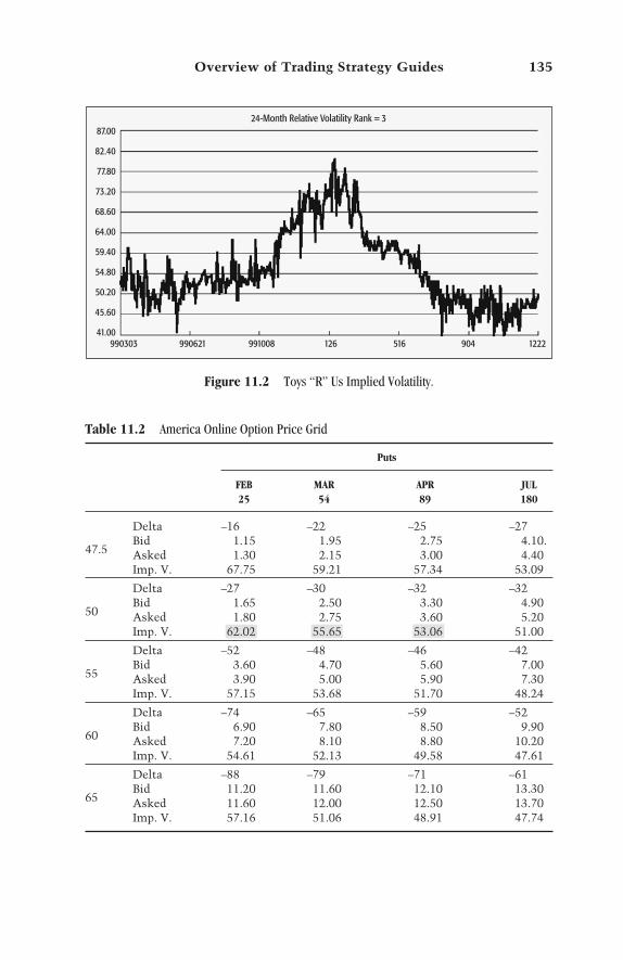
Table 11.2 America Online Option Price Grid
Puts
FEB MAR APR JUL25 54 89 180
Delta –16 –22 –25 –27Bid 1.15 1.95 2.75 4.10.
47.5 Asked 1.30 2.15 3.00 4.40Imp. V. 67.75 59.21 57.34 53.09
Delta –27 –30 –32 –32Bid 1.65 2.50 3.30 4.90
50 Asked 1.80 2.75 3.60 5.20Imp. V. 62.02 55.65 53.06 51.00
Delta –52 –48 –46 –42Bid 3.60 4.70 5.60 7.00
55 Asked 3.90 5.00 5.90 7.30Imp. V. 57.15 53.68 51.70 48.24
Delta –74 –65 –59 –52Bid 6.90 7.80 8.50 9.90
60 Asked 7.20 8.10 8.80 10.20Imp. V. 54.61 52.13 49.58 47.61
Delta –88 –79 –71 –61Bid 11.20 11.60 12.10 13.30
65 Asked 11.60 12.00 12.50 13.70Imp. V. 57.16 51.06 48.91 47.74
Overview of Trading Strategy Guides 135
87.00
82.40
77.80
73.20
68.60
64.00
59.40
54.80
50.20
45.60
41.00
24-Month Relative Volatility Rank = 3
990303 990621 991008 126 516 904 1222
Figure 11.2 Toys “R” Us Implied Volatility.

to make money. It also helps you visualize the worst-casescenario for the trade in question (Figure 11.3).
• Position-management considerations. Getting into a trade isoften the easy part. It can be more difficult to decide underwhat circumstances you should exit the trade. Each strategychapter contains a discussion of the most important position-management considerations for the selected trading strategyin general, and the example trade specifically.
As discussed in each strategy chapter, the key elements in-volved in using any strategy successfully are• When to consider using the strategy• When to enter a trade using the strategy• When to exit with a profit• When to exit with a loss
• Profit-taking and loss-cutting guidelines. Specific guidelinesare set for each example trade for determining when to exitthe trade. Specific rules are set for exiting with a profit andexiting with a loss. The trade exit criteria presented in eachchapter are not intended to serve as hard-and-fast rules but asguidelines to help you understand the importance and po-tential benefits of planning for the various contingencies as-sociated with each strategy.
136 The Option Trader’s Guide
3337
1112
–1112
–333728.87 32.19 32.50 38.88 42.19 45.50 48.88
Date: 4/20/01 Profit/Loss: 5 Underlying: 34.24 Above: 74% Below: 26% % Move Required: –12.0%
Figure 11.3 Reader’s Digest buy straddle risk curves.

• The end result of the example trade. Each example is carriedthrough to exit to help you see how the position-managementcriteria set forth when the trade was entered eventuallycaused the trade to be exited.
NOTE
The guidelines set forth in the following strategy chapters are not presentedas the only way to use a given trading strategy. In reality there is no single bestway to trade options. However, instead of attempting to enumerate the differ-ent ways in which a given strategy might be used, the goal here is to show youone specific method executed from start to finish.
Over the years it has been observed that traders who follow a structured,disciplined approach to trading generally have a great deal more successthan traders who make it up as they go along or who follow one set of rulesone time and a different set the next time. A set of specific trading rules doesnot always generate the maximum profit from a given trade or series oftrades. However, objective trading rules can keep a trader from making themajor mistakes that tend to doom traders who rely on gut feelings.
Whether you use the guidelines set forth in each strategy chapter or de-velop your own set of guidelines is not important. What matters is that yougain an understanding of the importance of setting objective entry and exitcriteria on an ongoing basis. In the long run, doing so gives you your best op-portunity to succeed.
Overview of Trading Strategy Guides 137
TEAMFLY
Team-Fly®


Chapter 12
BUY A NAKED OPTION
139
PURPOSE: To maximize the profitability of a market-timing call.
Key Factors
1. You have some reason to believe the underlying will move ina particular direction.
2. Low option volatility is a plus.3. Enough delta and time remain until expiration to minimize
time decay.
The strategy of buying a naked option is strictly a play on mar-ket timing. If your timing is good, you have the opportunity toleverage your gains by buying a call or put option rather thansimply buying or selling short the underlying security. In fact,the only reason to consider buying a naked call or put option isthat you expect a significant price movement by the underlyingsecurity within a specific time frame. Please note, however, thatalthough market timing is a key element in implementing thisstrategy, it is not the only important factor.
The primary mistakes traders make when buying calls andputs are

• Relying solely on market timing to trade options• Always buying out-of-the-money options hoping for the big
score• Buying options when implied volatility is high• Buying options with little time left until expiration
Poor timing, time decay, and a decline in implied optionvolatility are the greatest enemies of option buyers.
Poor timing will undo a naked long call or put position everytime. If you buy a call option and the underlying security de-clines significantly in price and does not rebound, you will in-variably suffer a loss. The same will happen if you buy a putoption and the price of the underlying security advances sharplyand does not pull back. Therefore, it is imperative that you buynaked calls and puts only when you have a solid reason for be-lieving that the underlying security is going to move in a partic-ular direction.
Time decay can eat away a large portion of the option pre-mium you pay if the underlying security fails to make the ex-pected move within a relatively short period. If you buy anoption whose price contains a great deal of time premium andvolatility subsequently declines, the time premium built intothe price of your option will decline, thus requiring an evengreater move by the underlying to compensate. If your markettiming is right, you may occasionally be able to get away withbuying high-priced (i.e., high-volatility) options. However, if youbuy out-of-the-money options often enough when volatility ishigh, the odds will invariably catch up with you.
In the long run it is critical to minimize the potentiallynegative effects of time decay.
To put the odds in your favor when buying naked options,use the following rules:
140 The Option Trader’s Guide

• Buy naked options only when you expect a significant pricemovement.
• Purchase options with a delta of 50 or more (for calls) and adelta of –50 or less (for puts).
• The lower the implied volatility, the better. Lower volatilitymeans less time premium. However, this does not mean thatyou should never buy options if volatility is high. Rather, thehigher the implied volatility, the further in the money andthe shorter term the option you buy should be. This mini-mizes the amount of time premium you pay and reducesyour exposure to time decay and a sharp decline in volatility.
• Buy options with at least 30 days (and preferably more) untilexpiration.
Following these rules will greatly improve your odds of successin the long run.
Two key elements to look for when selecting buy-naked-option trades are
1. Some catalyst to make you believe that a large price move isimminent
2. A way to take advantage of the expected move without beinghurt by time decay or a decline in volatility after the trade isentered
Market timing is discussed in Chapter 8. For no other strat-egy is timing more important than when buying a naked call orput. The specific timing method used may vary from trader totrader.
Regardless of which timing method you use, there is noreason ever to buy a naked call or put option if you do nothave some objective grounds for believing that the un-derlying security is about to make a significant move inprice. Also, buying naked options when implied volatilityis low increases your probability of profit by allowing youto buy cheap options.
Buy a Naked Option 141

Buying naked options when volatility is low gives yougreater upside potential, as well as the opportunity to profitshould option volatility increase in the near future becausehigher implied volatility translates into higher option prices. Ifvolatility is high, you must take steps to minimize the amountof time premium you pay.
One use of options is to pick tops and bottoms while limitingyour risk to a predetermined amount. Because of the limited-riskaspect of buying options, you can make a bet on a market top orbottom and simultaneously limit your risk to the amount youpay for the option if your timing turns out to be wrong.
Near the far right of the graph in Figure 12.1 is a solid downarrow on February 6, which indicates that a mechanical tradingsystem has generated a signal to buy puts on JDS Uniphase (sym-bol: JDSU). In Figure 12.2, you can see that option volatility forJDSU options is neither extremely high nor extremely low. Nev-ertheless, with a relative volatility rank of 6, we know that theoptions are not cheap and that if we buy puts and volatilityfalls sharply, the price of the option could be adversely affected.Table 12.1 shows that the choices are to buy a March optionwith 39 days until expiration, a June option with 130 days, or aSeptember option with 221 days. The February options will suf-fer the most from time decay since they expire the soonest.
142 The Option Trader’s Guide
11794
10445
9096
7747
6398
5049
3700918 1010 1101 1127 1220 10116 10208
Figure 12.1 A buy puts signal for JDS Uniphase on February 6.

However, the time premium in the longer-dated options couldcollapse if volatility levels fall. With the relative volatility rankat 6, there is definitely room for volatility to fall. A sharp declinein volatility would cause the June and September options to losea great deal of time premium. This combination of factorssuggests that buying an in-the-money March option and sellingit ahead of the last two weeks before option expiration is thebest play. This limits the amount of time premium paid up frontand thus limits the amount by which time decay can hurt thisposition.
With current option volatility in the middle of its historicalrange, Figure 12.2 shows a current relative volatility rank of 6. Ifwe buy options here, we hope that volatility will rise, thus in-flating the price of the option. However, we must also recognizethat a sharp drop in volatility is a possibility.
Table 12.1 shows that the March 65 put has a delta of –72.This means that this option will move 0.72 points for every onepoint move in the underlying stock. This value also indicatesthat there is approximately a 72% probability that this optionwill be in the money—and thus retain some intrinsic value—atthe time of March expiration. Most importantly, this option has
Buy a Naked Option 143
113.00
106.70
100.40
94.10
87.80
81.50
75.20
68.90
62.60
56.30
50.00
24-Month Relative Volatility Rank = 6
990706 991008 114 420 726 1101 10206
Figure 12.2 JDS Uniphase implied volatility (not exorbitantly high, but not low).

only 1.69 points of time premium built into it. For a put optionthis amount is calculated as follows:
Current stock price – (strike price minus option price) OR51.81 – (65 – 14.88) =51.81 – 50.12 = 1.69
144 The Option Trader’s Guide
Table 12.1 JDS Uniphase Puts: Priority Is to Minimize Effects of Time Decay and a Declinein Volatility
Puts
FEB MAR JUN SEP10 39 130 221
Delta –16 –25 –28 –27Bid –75 2.62 6.12 8.62
45 Asked 1.00 3.00 6.50 9.00Imp. V. 100.51 90.16 85.38 85.83
Delta –37 –38 –36 –33Bid 2.25 4.62 8.50 11.25
50 Asked 2.50 5.00 8.88 11.75Imp. V. 96.18 87.75 83.87 85.54
Delta –61 –51 –43 –38Bid 4.75 7.25 11.12 13.75
55 Asked 5.12 7.75 11.62 14.50Imp. V. 89.12 85.79 81.95 83.05
Delta –79 –63 –50 –44Bid 8.50 10.50 14.25 17.00
60 Asked 9.00 11.00 14.75 17.50Imp. V. 86.41 83.05 80.88 82.29
Delta –90 –72 –56 –49Bid 13.00 14.38 17.50 20.12
65 Asked 13.75 14.88 18.25 21.12Imp. V. 92.23 82.15 79.44 81.76
Delta –96 –80 –62 –53Bid 18.00 18.75 21.38 23.75
70 Asked 18.50 19.25 22.12 24.50Imp. V. NA 84.08 80.04 80.80

Many traders are reluctant to buy high-priced, deep-in-the-money options (this is not surprising because deep-in-the-moneyoptions cost more and offer less leverage). However, even ifvolatility falls sharply, only a small part of this option price willbe affected because this option has only 1.69 points of time pre-mium built into its price to begin with. Because volatility hasroom to fall, buying this particular option allows us to insulateourselves from the potentially negative effect of a decline involatility. In other words, no matter how far volatility levelsmight fall, this option can lose no more than 1.69 points as a re-sult of that decline.
Figure 12.3 depicts risk curves for four dates leading up toMarch 2, which is two weeks before March option expiration.With JDS Uniphase trading at a price of 51.81, we purchased twoMarch 65 put options at a price of 14.88 each (or $1487.50 peroption). As a result, our total dollar risk for this trade is $2975. Inother words, if we hold this option until expiration and JDSU istrading at 65 or above at that time, the March 65 put option willexpire worthless and we will sustain a loss of $2975 dollars. Thisis our worst-case scenario for this trade.
Buy a Naked Option 145
2648
883
–883
–264836.81 41.81 46.81 51.81 56.81 61.81 66.81
Date: 3/2/01Profit/Loss: 4Underlying: 50.01
Above: 55%Below: 45%
% Move Required: –2.9%
Figure 12.3 Buy 2 JDSU March 65 put options.
The graph in Figure 12.3 also depicts the negative effect oftime decay. Note how the lines keep shifting lower and to theleft with the passage of time. This has the effect of moving ourbreak-even point further away as option expiration draws closer.To dampen the inevitable negative effects of time decay, we pur-chased a deep-in-the-money put option (a strike price of 65 withthe underlying trading at 51.81) with a delta of –72.
If we were to hold this position until option expiration, ourbreak-even price would be 50.12. A close below that price at thetime of option expiration would result in a profitable trade. Aclose above that price at the time of option expiration would re-sult in a losing trade, assuming we are still holding the option atthat time. When this trade is entered the probability of JDSUbeing at or below our break-even price of 50.12 at the time of op-tion expiration is 44%. If the stock falls below 50.12, we willenjoy point-for-point profit. In other words, for each point thatthe stock declines, the put option will gain one point.
Because you pay time premium on top of any intrinsicvalue to purchase an option, whenever you buy a nakedcall or put you have less than a 50% probability of mak-ing money if you hold the trade until expiration.
This key piece of information goes a long way toward ex-plaining why so many traders lose money simply buying callsand puts. If you are always trading with a probability less than50:50, it can be extremely difficult to make money in the longrun. This does not mean that you should never buy naked op-tions, it simply illustrates the importance of considering otherstrategies when conditions warrant.
Position Taken
Buy 2 March 65 puts at 14.88.
Maximum risk –$2975Delta –72 × 2Days to expiration 39
146 The Option Trader’s Guide

Probability of profit 44%Current underlying price 51.81Break-even price at expiration 50.12
The maximum risk on this trade is $2975. In the worst-case sce-nario (i.e., if the stock price goes up rather than down), we couldsimply hold this trade until expiration and lose no more thanthat amount no matter how far JDSU may rise. If we are notwilling to risk the full $2975, we must devise a plan for cuttingour loss. Also, in case JDSU falls in price, we need to devise aplan for determining when to take our profits.
There are no magic formulas for determining when to cuta loss. What is important is planning in advance to dealwith your worst-case scenario.
Planning how to deal with the worst case is your only safe-guard against emotional decision making, which can lead to dev-astating losses.
Here are two workable approaches in this case:
1. Choose some arbitrary dollar amount and place a stop-lossorder at the appropriate price.
2. Figure 12.1 shows that JDSU recently hit a price of 64 andthen fell sharply. We can use this price as a resistance pointand decide that if the stock rallies above this point, our bear-ish outlook is wrong and we should exit the trade. While thisis not an exact science, the rationale is easy to understand.The reason that we got into the trade in the first place is be-cause we expect the stock to trend lower. If it rallies insteadand takes out a key resistance price, our basis for entering thetrade is no longer valid and we should exit.
For our purposes, we chose to hold the trade as long as JDSUstays below 64. Looking at the risk curves in Figure 12.3 we seethat if JDSU rallied to 64 prior to March 2, we would lose be-tween $1600 and $2100, depending on how soon the rally takesplace. The loss becomes a little greater with each passing weekdue to time decay.
Buy a Naked Option 147
TEAMFLY
Team-Fly®
For taking a profit, it is wise to employ a staggered technique.This simply means that we will take some profits at the firstgood opportunity and then attempt to let our profits run on theremaining position.
• If an oscillator becomes oversold, we will sell one put to lockin a partial profit.
• We will look to exit the position entirely on or very soonafter March 2. After that date we will want to exit the tradecompletely or roll out to another month. The reason forthis is that the March options expire on March 16, and wewould prefer to avoid holding a March option during the twoweeks before expiration. As discussed in Chapter 5, timedecay accelerates rapidly during the final two weeks beforeexpiration.
There is no way to guarantee that this approach will maxi-mize our profits or minimize our losses. Nevertheless, by havinga predetermined plan for exiting the trade, we can avoid the emo-tional pitfalls that cause so many traders to freeze at exactly thewrong time.
Position Management
Stop-loss:
• Sell 2 March 65 puts if JDSU exceeds 64.• Exit this trade after March 2.
Profit-taking:
• Sell 1 March 65 put if oscillator becomes oversold.• Exit this trade after March 2.
As you can see on the graph in Figure 12.4, this trade couldnot have worked out much better. After only three days in thetrade JDSU fell to 42.62 and became oversold. We were able tolock in a partial profit of $750 by selling one March 65 put at aprice of 22.38.
148 The Option Trader’s Guide

After a brief one-day rally four days later, the stock thenplummeted to 26.40 by March 2, allowing us to sell the secondMarch 65 put at a price of 38.25, for a profit of $2338. In sum,this trade garnered a profit of $3088 on an initial investment of$2975, or a return of 104% (Table 12.2). Before you get stars inyour eyes, you should realize that only a small percentage oftrades work out as well as this one did. The purpose here is notto say, “Wow, look at this great trade!” but to illustrate the crit-ical steps involved in trade selection and planning.
It should be noted that the return on this trade could havebeen much higher if we had bought lower-priced out-of-the-moneyoptions instead of the deep-in-the-money 65 puts. However,hindsight is always 20/20. At the time of the original signal ourgoal was not to throw caution to the wind and reach for the max-imum profit. What we sought was a reasonable tradeoff betweenreward and risk.
This trade was entered into on the basis of a mechanical trad-ing system. As with most systems, sometimes the signals are
Buy a Naked Option 149
Table 12.2 JDSU March 65 Puts
Long/Short Quantity Type Price In Last Price $ + /–
Long 1 March 65 put 14.88 22.38 +$750Long 1 March 65 put 14.88 38.25 +$2338
10880
9476
8072
6668
5264
3860
24561106 1122 1213 10103 10123 10212 10302
Figure 12.4 JDSU Price Falls, Generating a Profit for March 65 Puts.
good and sometimes they are not. In a nutshell, we were willingto risk a sum of money (approximately $2100 if JDSU had ralliedto 64) on a speculative bet that JDSU would fall in price. We alsoassessed the risk on this trade and took steps to minimize ourrisk by limiting the amount of time premium we paid and by set-ting some objective and specific stop-loss criteria.
The key point to note in this example is the importance ofplanning ahead to deal with both favorable and unfavorable sit-uations. On one hand this can be viewed as a good trade becauseit made money. However, even if this trade had gone the otherway, the loss would have been limited to an amount that wewere willing to risk at the time the trade was entered.
Trade Result
Sold 1 March 65 put at 22.38.Sold 1 March 65 put at 38.25.
Profit = $3088
150 The Option Trader’s Guide
KEY POINTS
If you feel compelled to pick a top or bottom, options—by virtue of their lim-ited risk—can give you a great deal more staying power than would tradingthe underlying security. Nevertheless, if the reason you picked a top or bot-tom in the first place is no longer valid, you may consider cutting your lossand moving on rather than hoping that things will turn around.
The Great Paradox of Option Buying
Lesson AThe way to maximize your profitability on any single trade is to buy a far out-of-the-money option.
Lesson BThe way to maximize your profitability in the long run is to avoid Lesson A.

Chapter 13
BUY A BACKSPREAD
151
PURPOSE: As an alternative to buying naked calls orputs, buying a backspread affords the opportunity toprofit from a market-timing call with some protection ifwrong. It is also a good way to take advantage of lowvolatility.
Key Factors
1. You are expecting a particular market movement but wantsome protection if you are wrong.
2. There is low implied volatility (you hope volatility will riseafter the trade is entered).
3. The ability to enter at a credit or a favorable volatility skewis a plus.
The strategy of buying a backspread involves writing an at-the-money or in-the-money call or put option and simultaneouslybuying a greater number of out-of-the-money options. (The ratioof options bought to options written can be 2:1, 3:2, 5:3, 11:10, orany other combination. The main point is that you buy more op-tions than you write.) Ideally this trade is entered at a credit (i.e.,you take in more money for the options you sell than you payout for the options you buy), which offers you complete protec-tion if your expected scenario turns out to be exactly wrong.
The backspread strategy can be used in a number of situa-tions. Under the right circumstances this strategy is ideal fortimes when you feel compelled to pick a top or bottom but areconcerned about the risk if you are wrong. It can also be used asan alternative to buying a naked call or put option if you expecta particular underlying price movement but are concerned thatthe move may not take place soon enough to keep a naked call orput option from experiencing serious time decay. There are twosituations that generally offer the best opportunities for usingbackspreads.
1. Situation A. One use of this strategy is to enter a backspreadwhen a given stock or futures market is experiencing a steep de-cline (or a sharp rally) that you think could reverse sharply at anytime. If you buy a naked call option in this situation and the de-cline continues, you may very quickly find yourself with a largeloss and thus in need of a major rally simply to get back to break-even. In this situation, buying a backspread can give you a greatdeal more staying power than buying a naked option because itoffers you some protection on the downside.
For example, say a stock you are following is plummetingand you believe that it is extremely oversold and due for a sharprally. You might sell an at-the-money call option for 5.00 pointsand buy 2 one-strike, out-of-the-money options for 2.00 pointseach, or 4.00 points total. The end result is that you receive a netcredit of 1.00 point ($100). Because you are long more calls thanyou are short, you have unlimited upside potential if you arecorrect and the stock rallies. If you are dead wrong and the stockcontinues to dive, you still stand to make $100 by virtue of tak-ing in more premium than you paid out.
2. Situation B. You expect a particular stock or futures marketto stage a substantial rally (or decline) but are concerned that itmay take a while to play out. One benefit of a backspread (bar-ring a sharp decline in option volatility) is that if it is properlyconstructed, it can give you very little dollar risk for a relativelylong period. Thus, you retain the potential for unlimited profit,you have downside protection if the underlying security goes inexactly the opposite direction of what you expect, and you may
152 The Option Trader’s Guide

have little dollar risk for a lengthy period, even if the underlyingfails to make a substantial move in either direction.
Whatever the situation, it often pays to use longer-dated op-tions when trading a backspread. This gives you more time for amove to play out. Additionally, longer-dated options react moreto changes in volatility. Thus, if you enter a backspread whenvolatility is very low, you have the potential to achieve windfallprofits if volatility subsequently rises.
As with all option strategies, there is no free lunch. If the un-derlying security remains relatively unchanged or impliedvolatility declines sharply, this trade can generate losses.
The majority of the risk associated with a backspread oc-curs if this trade is held until expiration.
That is why it is recommended that backspreads not be helduntil expiration if the underlying security is trading within aprice range that could result in substantial loss at expiration. Forexample, let’s assume that based on the formation in the barchart in Figure 13.1, we believe that Toys “R” Us has made a
Buy a Backspread 153
Figure 13.1 Toys “R” Us daily price.
1996
1905
1814
1723
1632
1514
1450803 825 919 1012 1106 1129 1222

Table 13.1 Toys “R” Us Option Prices
Calls
JAN FEB MAR JUN27 55 84 175
Delta 95 90 87 83Bid 3.25 3.37 3.50 4.00
12.5 Asked 3.50 3.62 3.75 4.37Imp. V. 70.27 56.24 51.18 51.88
Delta 65 64 63 64Bid 1.25 1.56 1.87 2.43
15 Asked 1.44 1.75 2.06 2.68Imp. V. 56.02 51.49 51.49 47.79
Delta 24 33 37 44Bid .25 .56 .81 1.43
17.5 Asked .38 .75 1.00 1.62Imp. V. 52.36 52.15 50.38 47.83
Delta 5 13 18 28Bid .00 .06 .31 .75
20 Asked .06 .18 .43 1.00Imp. V. 53.04 44.25 49.70 47.72
bottom and will soon stage a rally. This part of the analysis isbased on whatever timing technique an individual trader decidesto use and thus will vary from trader to trader. In this case we aretrading based on a chart pattern involving a double bottom and akey reversal day.
One alternative would be to buy a naked call option. Thatwould give us unlimited profit potential if Toys “R” Us doesrally, with limited downside risk. However, let’s say we are alsoconcerned that this recent bottom will not hold and that the re-cent advance is just a rally in a bear market. Given these con-cerns, an alternative would be to write the the June 12.5 call andto buy a higher strike price (the June 17.5) in a ratio that resultsin receiving a credit by virtue of taking in more premium for theoption we write than we pay out for the options we buy. In thisexample, a trade can be entered at a slight credit by writing 5 ofthe 12.5 calls and buying 11 of the 17.5 calls, as shown in Table13.1.
The ideal circumstance for using a backspread is when youcan write an option that is trading at a significantly higher im-
154 The Option Trader’s Guide

plied volatility than the option you buy. This gives you yourgreatest potential edge. At a minimum, you should look for anopportunity to write an option trading at a higher implied vola-tility than the option you plan to buy. The preceding examplemeets this minimum criteria (the 12.5 call is trading at an im-plied volatility of 51.88, and the 17.5 call is trading at an impliedvolatility of 47.83).
In sum, the backspread strategy can give a trader
• The courage to pick a top or bottom in the face of a stronglytrending market
• The time to allow a market-timing call to work out withoutbuying a naked call or put option
• The potential to profit from a significant increase in volatility
The trade shown in Figure 13.2 is entered on December 22using June options. We will hold this trade for up to three monthsand hope for a large price movement and an increase in volatility.Option volatility for Toys “R” Us is currently at the low end ofits historic range. It is certainly possible that volatility could fall
Buy a Backspread 155
24-Month Relative Volatility Rank = 387.00
82.40
77.80
73.20
68.60
64.00
59.40
54.80
50.20
45.60
41.00990303 990621 991008 126 516 904 1222
Figure 13.2 Toys “R” US implied volatility.

back within the 40 to 50 range and stay there for an extended pe-riod. Nevertheless, there is clearly room for volatility to rise if thestock starts to move. As we will illustrate, a rise in volatility canhave an extremely beneficial effect on a backspread.
The graph in Figure 13.3 shows risk curves for three dates—January 20, February 20, and March 20. With Toys “R” Us trad-ing at 15.69, we purchased 11 June 17.5 call options each at aprice of 1.62 and simultaneously wrote 5 June 12.5 call optionsat a price of 4.00.
This trade nets an initial credit of $212, which represents themaximum profit potential if we were to hold this trade untilJune expiration and Toys “R” Us was trading below 12.5. If Toys“R” Us rallies sharply, we have unlimited profit potential byvirtue of being long more call options than we are short. In con-trast, if Toys “R” Us resumes its recent downtrend and declinessharply, we still stand to profit by virtue of having received theinitial $212 credit when we entered the trade. In reality we willnot likely collect this amount since we are only planning to holdthe trade for a maximum of three months.
If this trade is held for three months—barring any changes inimplied volatility—our break-even points are 10.04 on the down-side and 19.30 on the upside.
156 The Option Trader’s Guide
3070
1876
682
–5125.68 9.00 12.31 15.69 19.00 22.31 25.69
Figure 13.3 Toys “R” Us backspread.

Each risk curve drawn on the graph in Figure 13.3 shows thepotential profit or loss as of a given date based on the price ofToys “R” Us (the current price of 15.69 is in the middle, withplus or minus 10-point increments on either side). A close ex-amination reveals that the dollar risk increases with each line(i.e., as time decay begins to work against us) if the stock stays ina narrow range. The maximum risk on this trade of $2266 wouldbe experienced only if we held this position until expiration andToys “R” Us closed at exactly 17.5. This graph illustrates theone negative to using the backspread strategy: If the marketmakes a decent move up or down, that’s fine. The primary riskassociated with this trade is that Toys “R” Us might simply driftwithin a narrow range.
Position Taken
Sell 5 June 12.5 calls at 4.00.Buy 11 June 17.5 calls at 1.62.
Credit obtained $212Current underlying price 15.69Days to expiration 175Break-even price at expiration Below 10.40 or
above 19.30
Before following this trade through until exit, let’s examine afew other factors affecting backspreads in general.
Backspreads versus Naked Calls and Puts
Backspreads are generally used in place of buying a naked call orput option. Option trading involves many tradeoffs, and back-spreads are no exception. If you use a backspread instead of buy-ing a naked call option, you gain certain advantages but you alsogive up something to gain these advantages.
The primary difference between these two positions is whathappens if the stock goes down. Figure 13.4 depicts the risk
Buy a Backspread 157
TEAMFLY
Team-Fly®

curves for a trader buying 3 March 15 calls at 2.06. At any pricebelow 17.06 this trade will show a loss and at any price below 15it will lose 100%. Conversely, the backspread shown in Figure13.5 will lose less money as the stock falls and could eventuallyearn a profit if the stock falls far enough.
158 The Option Trader’s Guide
2604
1447
289
–8685.68 9.00 12.31 15.69 19.00 22.31 25.69
Date: 3/16/01 Profit/Loss: –2 Underlying: 17.16 Above: 35% Below: 65% % Move Required: +9.1%
Figure 13.4 Toys “R” Us buy 3 March 15 calls at 2.06.
3070
1876
682
–5125.68 9.00 12.31 15.69 19.00 22.31 25.69
Date: 3/16/01 Profit/Loss: –4 Underlying: 19.38 Above: 1% Below: 99% % Move Required: +24.7%
Figure 13.5 Toys “R” Us backspread risk curves.

Volatility and Backspreads
The advantage to entering a backspread when volatility is low isthat you can gain additional profit if volatility rises after youenter the trade. This trade was entered on December 22. Figure13.6 shows the expected return as of March 16 if volatility is un-changed from its level when the trade was entered. Figure 13.7depicts the expected returns based on three volatility levels as ofMarch 16. The lowest curve represents expected return if volatil-ity falls to 40, the middle curve represents a volatility of 60, andthe uppermost curve represents volatility rising to 80 threemonths from now. To fully appreciate the impact of volatility,let’s assume that the stock is trading at 19 on March 16. At avolatility of 40, the trade would show a loss of $490. At a volatil-ity of 60 the trade would show a profit of $180. At a volatility of80 this trade would show an open profit of $795. The upside po-tential created by a rise in volatility is the reason you should ide-ally enter backspreads when volatility is low. Also, rememberthis can work against you in reverse. If you enter a backspreadwhen volatility is very high and volatility subsequently col-lapses, the expected return on your trade will likely plummetalso.
Buy a Backspread 159
2828
1571
314
–9435.68 9.00 12.31 15.69 19.00 22.31 25.69
Date: 3/16/01 Profit/Loss: –2 Underlying: 19.27 Above: 18% Below: 82% % Move Required: +22.1%
Figure 13.6 Toys “R” Us backspread risk curvess (3 months later if volatility is unchanged).

Managing a backspread position can be extremely subjective.First, you have unlimited profit potential on one side and a de-fined profit potential on the other side. Also, you must be con-cerned about time decay, particularly, the longer the trade goeson with the underlying drifting in a narrow range. The other con-cern is the prospect of getting assigned on the option you write.If the underlying moves far enough in the expected direction, theoption you wrote will eventually trade deep in the money. Asthe amount of time premium narrows, the likelihood of exerciseand assignment becomes greater. For purposes of setting objec-tive position-management rules for this trade, we will first lookat what we know for sure about this trade. The two things weknow for sure are that
1. Our profit potential on the downside is $212.2. Our maximum risk is $2268 and can occur only if we hold
this trade until expiration. The effect of time decay can beseen in Figure 13.8, which shows risk curves as of February15, April 15, and June 15 (option expiration). Notice how riskincreases significantly at expiration.
160 The Option Trader’s Guide
3409
1894
379
–11375.68 9.00 12.31 15.69 19.00 22.31 25.69
Date: 3/16/01 Profit/Loss: 1917 Underlying: 22.34 Above: 5% Below: 95% % Move Required: +42.9%
Figure 13.7 Toys “R” Us backspread (3 months later if volatility is at 80, 60, or 40).

Our first step is simply to decide that we will not hold thistrade until expiration. This relieves any worry about experienc-ing the maximum potential loss. The good news regarding thistrade is that unless volatility plunges to new lows, there is al-most no way to lose a lot of money for at least the next threemonths because volatility is already low and there is a great dealof time left until expiration. We will hold this trade for a maxi-mum of three months.
Looking at the historical volatility for Toys “R” Us, we cal-culate that a two-standard-deviation move for Toys “R” Us overa 90-day period would be 5.64 points. In other words, if Toys “R”Us falls to 10.04 or rises to 21.33 at any time during the nextthree months, this would constitute a statistically significantmove for this stock. As a result, we decide to close the trade if ei-ther of these price levels is pierced. Looking again at the riskcurves in Figure 13.4, we can see that if the stock fell to 10.04 thetrade would be about at break-even, and the stock would thenhave to rally significantly to achieve a meaningful profit. We arehoping that the Toys “R” Us price will rally. If, however, thestock collapses later on and we have the opportunity to get out
Buy a Backspread 161
3004
1168
–668
–25045.68 9.00 12.31 15.69 19.00 22.31 25.69
Date: 6/15/01 Profit/Loss: –2268 Underlying: 17.51 Above: 37% Below: 63% % Move Required: +11.7%
Figure 13.8 Toys “R” Us as of 2/15, 4/15, and 6/15 (expiration).

at about break-even, we will take the opportunity to do so. No-tice in Figure 13.4 that if we had bought naked calls and thestock collapsed, we would be faced with a large percentage loss.
If the stock rallies to 21.33 within the next three months, wecan anticipate a profit of $700 to $1700, depending on how soonthe rally takes place and the level of volatility at the time ourtarget price is reached.
Position Management
Trade exit criteria:
• If Toy “R” Us rallies to 21.33 or falls to 10.04, exit the entiretrade.
• If neither target is hit within three months, exit the entiretrade.
As you can see in Figure 13.9, Toys “R” Us shot higher inearly January, closing on January 4 above our upside target of21.33. This trade could have been closed out on January 4 for aquick profit of $1443 (see Table 13.2). Obviously, not every tradewill work out this well or this quickly.
Nevertheless, this example illustrates two key factors in op-tion trading success:
1. The importance of recognizing each trade’s weak spot2. Planning in advance to deal with the worst-case scenario
In this example, we felt that Toys “R” Us had bottomed out,but we were not highly confident that the recent low wouldhold. This is why we used the backspread strategy rather than
162 The Option Trader’s Guide
Table 13.2 Toys “R” Us Backspread
Long/Short Quantity Type Price In Last Price $ + /–
Short 5 June 12.5 calls 4.00 10.75 –$3375Long 11 June 17.5 calls 1.62 6.00 +$4818

simply buying a naked call. We also recognized that the worstcase would occur if Toys “R” Us drifted in a narrow range. Tolimit our dollar risk under such circumstances, we bought op-tions with six months left until expiration and planned to exitthem after only three months.
The purpose of this example is not to show you how easy itis to make money trading options. The purpose is to emphasizethe benefits of intelligent position management. Too manytraders put on a trade like this and simply wait to see what hap-pens. This is usually a mistake. It will be very beneficial to yourlong-term results if you always have a plan when you enter anytrade. This includes setting criteria for deciding when to take aloss. It is no fun to lose money in trading, but the fact remainsthat cutting a loss and moving on is very often the proper moveto make. It is much easier to implement this important step ifyou have planned in advance to cut your loss based on some rea-sonable criteria rather than to react by making an emotional de-cision to an adverse price movement after the fact.
If you already know when you enter a trade what has to hap-pen for you to exit, the number of mistakes you make in tradingwill decline significantly.
Buy a Backspread 163
2668
2465
2262
2059
1856
1653
1450901 926 1018 1110 1206 1229 10129
Figure 13.9 Toys “R” Us rallies to upper price target.

Trade Result
Upside target of 21.33 exceeded on January 4.Profit = $1443
KEY POINT
Do not plan on holding a backspread position until expiration. Exiting thetrade before expiration guarantees that you cannot sustain the maximumpotential loss.
164 The Option Trader’s Guide

Chapter 14
BUY A CALENDAR SPREAD
165
PURPOSE: To take advantage of differences in optionvolatilities.
Key Factors
1. The option sold should be trading at a volatility at least 15%higher than that of the option bought.
2. Do not use this strategy if option volatility is high (the lowerthe volatility, the better).
3. No more than 45 days remain until the option sold expires.4. You have some reason to believe the underlying will remain
within a particular range of prices.
One area of opportunity unique to option trading is that eachoption for a given underlying security generally trades at a dif-ferent implied volatility level. Sometimes the disparity betweenthe volatility of different options can be quite large. This situa-tion gives alert traders the opportunity to take advantage of dis-parities between the implied volatility levels of different options.The idea is simply to write an option that is trading at a signifi-cantly higher implied volatility than the option you buy.
One way to take advantage of a large disparity in volatility isto buy an option that is trading at a given implied volatility leveland simultaneously write a different option that is trading at a

much higher implied volatility. This gives you an edge becauseyou are buying a cheaper option and selling a more expensive op-tion. Whenever you trade a spread, you should look for an op-portunity to write an option trading at a higher volatility thanthe option you buy. This type of opportunity is also discussed inChapter 13, Buy a Backspread, and Chapter 16, Sell a VerticalSpread. Each of these strategies trade different options withinthe same expiration month. Another useful way to take advan-tage of volatility disparities is by trading a calendar spread.
A calendar spread is entered into by buying one option of agiven strike price and expiration month and simultaneouslywriting an option with the same strike price but a different ex-piration month that has less time until expiration than the op-tion you bought. Buying a July 50 call option on a particularstock and simultaneously selling a June 50 call option is an ex-ample of a calendar spread.
As a rule of thumb, the time to enter a calendar spread iswhen a near-term option is trading at an implied volatil-ity that is at least 15% above the implied volatility of thefarther-out option of the same strike price.
A calendar spread is a neutral position. In other words, youbenefit from having the underlying security remain within a par-ticular range of prices and by allowing time decay to work inyour favor. The width of this profitable range of underlyingprices is determined by the difference in the implied volatilitylevels of the options used. Thus, the higher the implied volatil-ity of the option sold relative to the implied volatility of theoption bought, the higher the probability of profit.
A calendar spread is a limited-risk position, but there are twodangers in trading a calendar spread. First, if the underlying se-curity advances or declines significantly, this trade can becomevery unprofitable. Second, a major decline in option volatilitycan put you in a position in which you have little or no chanceof making money (more on this topic later).
The less time left until expiration for the options you sell,the better (assuming you receive enough premium to make the
166 The Option Trader’s Guide

trade worth taking in the first place). In addition, by trading op-tions with deltas between 35 and 65 for calls and from –35 to –65for puts, you can establish a range of underlying prices aboveand below the current price that can yield a profitable trade. Out-side of these delta values you can get into a situation in whichthe underlying security must make a fairly substantial move inprice to generate a profit, which can greatly reduce your proba-bility of profit. The exception to this rule is that you can trade astrike price that is within one strike price of the underlying se-curity price, regardless of the deltas of the options involved.
To maximize your potential when trading calendar spreads:
• Enter a calendar spread only when the option you sell is trad-ing at an implied volatility at least 15% above the impliedvolatility of the option you purchase.
• Trade calendar spreads only when the relative volatility rankis below 6 (on a scale of 1 to 10). The ideal situation is totrade a security with a relative volatility rank of 1 or 2 thatalso meets the other criteria. The reason for this suggestedcriterion is simply that if volatility increases after you entera calendar spread, you stand to reap windfall profits becausethe price of the longer-term option you bought will rise muchmore than the short-term option you wrote.
• Sell options with no more than 45 days (and preferably fewer)remaining until expiration.
• Trade options with delta values between 35 and 65 (calls) orfrom –35 to –65 (puts), or trade options that are no more thanone strike price away from the current underlying price.
Make certain that the overall level of option volatilities forthe underlying security is relatively low before entering a calen-dar spread. This is extremely important because a sharp declinein volatility has the potential to wipe out any chance you haveof making money when trading a calendar spread. Remember,you are paying more for the option you buy than you are receiv-ing for the option you write. In terms of its effect on optionprices, a decline in volatility lowers all boats. Therefore, ifvolatility falls dramatically, you have more to lose from a de-cline in the price of the option you bought than you do to gain
Buy a Calendar Spread 167
TEAMFLY
Team-Fly®

from a decline in the price of the option you sold. As a result, inorder to put the odds as far in your favor as possible you shouldfocus your search for calendar spreads on stocks or futures mar-kets with low relative volatility rankings.
In Table 14.1 and Figure 14.1 you see an ideal setup for a cal-endar spread using options on America Online (AOL).
• The near-term at-the-money put option (the February 50 put)is trading at an implied volatility level (62.02%) that is 17%higher than the implied volatility (53.06%) for the same op-tion two months out (the April 50 put).
• The overall level of option volatility for AOL is extremelylow (a relative volatility rank of 1).
168 The Option Trader’s Guide
Table 14.1 America Online Volatility Skew
Puts
FEB MAR APR JUL25 54 89 180
Delta –16 –22 –25 –27Bid 1.15 2.75 4.10
47.5 Asked 1.30 3.00 4.40Imp. V. 67.75 57.34 53.09
Delta –27 –30 –32 –32Bid 1.65 2.50 3.30 4.90
50 Asked 1.80 2.75 3.60 5.20Imp. V. 62.02 55.65 53.06 51.00
Delta –52 –48 –46 –42Bid 3.60 4.70 5.60 7.00
55 Asked 3.90 5.00 5.90 7.30Imp. V. 57.15 53.68 51.70 48.24
Delta –74 –65 –59 –52Bid 6.90 7.80 8.50 9.90
60 Asked 7.20 8.10 8.80 10.20Imp. V. 54.61 52.13 49.58 47.61
Delta –88 –79 –71 –61Bid 11.20 11.60 12.10 13.30
65 Asked 11.60 12.00 12.50 13.70Imp. V. 57.16 51.06 48.91 47.74

• There are only 25 days left until the February option expires.This means that the effect of time decay will begin to workin our favor quickly, which is ideal when writing options.
• The deltas for these options (–32 and –27) are outside the pre-ferred –35 to –65 range, but the options are within one strikeprice of the underlying price, so this trade still qualifies as aneutral trade.
One other favorable factor to look for when considering acalendar spread is an underlying security in a trading range. Foran example of a trading range market, look at the graph of AOLin Figure 14.2. In this graph you can see that AOL stock traded ina range of 31 to 62 for almost 4 months. In a properly constructedcalendar spread, you will generally not be at risk to lose a lot ofmoney unless the underlying security makes a significant pricemovement. Focusing on securities with easily identifiable sup-port and resistance levels above and below the current pricegives you a better chance of making money with calendarspreads. Underlying securities with established support and re-sistance levels are ideal candidates for calendar spreads becausethe underlying security is required to stage a breakout to a new(at least short-term) high or low for the trade to turn into a loss
Buy a Calendar Spread 169
Figure 14.1 America Online implied volatility.
24-Month Relative Volatility Rank = 1
90.00
85.30
80.60
75.90
71.20
66.50
61.80
57.10
52.40
47.70
43.00990412 990728 991112 301 619 1004 10122

of any meaningful size. Nevertheless, although support andresistance levels are important, the difference between thevolatility of the option you buy and the option you write re-mains the key element in selecting calendar spreads to trade. Atrading range is simply another favorable factor to look for.
As shown in Figure 14.3, using this strategy establishes a po-sition that will generate a profit only if the underlying securitystays within a particular range of prices. If the underlying secu-
170 The Option Trader’s Guide
6226
5716
5206
4696
4186
3676
3166927 1013 1102 1121 1211 10102 10122
Figure 14.2 America Online in a trading range.
2230
743
–743
–223036.84 42.50 48.19 53.81 59.50 65.19 70.81
Date: 2/16/01 Profit/Loss: 7 Underlying: 45.4 Above: 85% Below: 15% % Move Required: –16.1%
Figure 14.3 America Online calendar spread risk curves.

rity moves outside this range, losses will occur. The width ofthis profit range is determined by the size of the difference in theimplied volatility of the option bought versus that of the optionsold. This underscores the importance of having as wide a spreadas possible between the volatility levels of the option boughtversus the option sold.
NOTE
Before trading a calendar spread on a futures contract, you should make cer-tain that both the options you are going to use trade based on the same un-derlying futures contract month. For example, January, February, and MarchT-bond options trade based on the March T-bond futures. April, May, andJune options trade based on the June futures contract. You should not tradeone option based on the June futures and another option based on the Marchfutures because futures contracts of different months can trade independentlyof one another. This is especially true in the grain markets (e.g., Corn, Soy-beans, Wheat) and the soft markets (e.g., Coffee, Sugar). If you trade optionsbased on different futures months, you run the risk of losing money on bothoptions if the underlying futures contracts move in opposite directions. Forexample, it is not uncommon for July Soybeans to rally while November Soy-beans decline. If you were long a November call option and short a July calloption, you could end up losing money on both sides of the trade. Do notmake the mistake of putting yourself in this potentially dangerous situation.
The graph in Figure 14.3 displays risk curves for three datesleading up to option expiration. With AOL trading at 53.81, webought 10 April 50 puts at 3.60 and sold 10 February 50 puts at1.65. The cost of this position is $1995. Our maximum profit po-tential is approximately $2230. The amount of profit potential isonly an approximation because although we can state with cer-tainty how much the February option will be worth at the timeof February expiration at a given underlying price, we can onlyestimate the price at which the April option will be trading atthat time. This is because the volatility of that option may riseor fall in the meantime, thus inflating or deflating the price ofour long option accordingly.
Buy a Calendar Spread 171

Of key importance in viewing these risk curves (or the riskcurve for any calendar spread) is to note the break-even points.As you can see in Figure 14.3 (assuming no change in impliedvolatility levels), this trade will a show a profit at February op-tion expiration if the price of AOL is between 45.34 and 56.64.Based on the historic volatility of AOL stock when this tradewas entered, there is a 43% probability that the price of AOLwill be within this price range at the time of option expiration.
As always, there is no way to know in advance how this tradewill work out. All we can do is put the odds as much in ourfavor as possible. To that end, with this example trade we
• Chose a market with low option volatility (a relative volatil-ity rank of 1)
• Sold a call option with an implied volatility 17% higher thanthe volatility of the option we bought
• Sold a call option with less than 45 days until expiration (25days in this case)
In this trade we exceeded our target delta range (of –35 to –65when trading puts), but the strike price (50) is within one strikeprice of the current stock price (53.81)
The biggest risk we assume when entering this trade is thatAOL will trade outside the profit range of 45.34 to 56.64. Thekey question to answer when setting position managementcriteria is how to deal with this possibility. Our choices are asfollows:
• Establish some arbitrary stop-loss level.• Simply hold the trade until near expiration and hope that the
stock is within our profit range.• Establish some alternate exit criteria.
In this case we decided to hold the trade until expiration un-less one of the following two criteria is met:
1. If the time premium on the February 50 put declines to 0.125or less, we will exit the entire trade. If the stock falls and theshort February 50 put trades deep in the money, we will close
172 The Option Trader’s Guide
the trade to avoid being exercised on the short puts. If thestock rises and the amount of time premium built into theprice of the February 50 put falls to 0.125, we can either closeout the entire trade or buy back the February puts and con-tinue to hold the long April puts in hopes that AOL stockwill fall. This would be a subjective decision, however, andwould expose us to greater risk.
2. If the trade shows an open loss in excess of $1000, we willexit the trade. Inspecting the risk curves, we find that inorder for this loss level to be reached the stock price wouldhave to fall below 42 or rise above 62.50. Based on the his-toric volatility for AOL, the probability of this happening isonly about 26%.
Position Taken
Buy 10 April 50 puts at 3.60.Sell 10 February 50 puts at 1.65.
Approximate maximum profit $2230Approximate maximum risk –$1994Approximate probability of profit 43%Current underlying price 53.81Break-even price at expiration Above 45.34 and
below 56.64
Position Management
Stop-loss:
• If the time premium on the February 50 put declines to0.125, exit the entire trade.
• If the trade shows an open loss greater than $1000, exit theentire trade.
Profit-taking: As long as trade shows a profit, hold as close to ex-piration as possible.
Buy a Calendar Spread 173

As you can see in Figure 14.4, AOL stock rallied for a coupleof days after this trade was entered and then fell back below 50.Fortunately, it did not fall far enough to cause our short optionto trade deep in the money, so we were able to let the trade ride.At the close of the day before February expiration, the April putcould be sold at a price of 4.00, generating a profit of $400 on a10-lot. The February 50 put could be bought back at a price of0.75, generating a profit of $900 on a 10-lot. As a result, thistrade netted a profit of $1300 (Table 14.2).
Trade Result
174 The Option Trader’s Guide
5710
5286
4862
4438
4014
3890
31661113 1130 1220 10110 10130 10220 10309
Figure 14.4 America Online stays in profitable range.
Table 14.2 AOL Calendar Spread Result
Long/Short Quantity Type Price In Last Price $ + /–
Long 10 April 50 Puts 3.60 4.00 +$400Short 10 February 50 Puts 1.65 0.75 +$900
KEY POINT
The ideal time to enter a calendar spread is when the implied volatility of theoption you sell is at least 15% higher than the implied volatility of the optionyou buy.

A Decline in Volatility Is Deadly to Calendar Spreads
To understand why low volatility is one of the suggested guide-lines in selecting calendar spreads, you must understand the im-pact that changes in volatility can have on this type of spread. Ina calendar spread you are long an option that has more time leftuntil expiration than the option you are short. As discussed inChapter 6, the more time left until expiration, the more sensitivean option will be to changes in volatility. As a result, if volatilityrises after you enter a calendar spread, you stand to gain a wind-fall profit because that increase in volatility will serve to inflatethe price of the option you are long far more than it will the priceof the option you have written. Conversely, if volatility falls dra-matically after you enter a calendar spread, you stand to take un-expected losses because this decline in volatility will serve todeflate the price of the option you are long far more than it willthe price of the option you have written.
The graph in Figure 14.5 depicts three risk curves for theAOL calendar spread we just discussed. Each line represents theprofit or loss we could expect from this trade as of February op-tion expiration, depending on the level of implied option volatil-ity at that time.
Buy a Calendar Spread 175
4693
2346
0
–234736.84 42.50 48.19 53.81 59.50 65.19 70.81
Figure 14.5 America Online calendar spread (volatility of 83%, 63%, or 43%).

If you look again at Figure 14.1, you will see that impliedvolatility for AOL options had recently ranged as low as 43% andas high as 83%. In Figure 14.5 you can see three risk curves.Each curve represents the expected profit or loss from our calen-dar spread example trade, with the only difference being the levelof option volatility at the time of February option expiration.
• The upper curve depicts the profit or loss we could expect atthe time of February expiration if volatility rose back up toits most recent high of 83%.
• The middle curve is based on a volatility of 63%.• The lowest curve assumes that option volatility fell back to
its recent low of 43%.
Please take a moment to study these curves because they dra-matically illustrate why volatility is so important when tradingcalendar spreads.
Remember, at expiration the February call that we wrote willhave no time premium left, only intrinsic value. However, theprice of the April call option that we bought will be highly de-pendent on the level of volatility at that time. If volatility risesto high levels, the price of our long option will be inflated ac-cordingly. If volatility falls to lower levels, the price of our longoption will be deflated accordingly.
It would be optimistic to assume that volatility will rise backto its recent high of 83% after this trade was entered. Neverthe-less, it is important to understand the effect that such a rise involatility would have on our example trade. If the April 50 puttraded at a volatility of 83% at the time of February expiration,the break-even points on this trade would expand from 45.34 onthe downside and 56.64 on the upside to 39.61 on the downsideand 68.06 on the upside. As a result, the expected return ishigher at any underlying price, and the probability of profit soarsfrom 43% to 88%. Clearly an increase in volatility greatly en-hances the profit potential of this trade because it serves to in-flate the price of the option we bought.
At the other end of the spectrum, if volatility falls to 43%,the profit potential for this trade declines sharply (as depicted bythe lowest risk curve in Figure 14.5). In addition, the range of un-
176 The Option Trader’s Guide

derlying prices that will generate a profit contracts significantly.Accordingly, as volatility declines, our probability of profit isdramatically reduced.
In this example, if implied volatility fell from the currentlevel of 53% to 43%, AOL stock would have to be trading be-tween 47.25 and 53.50 at the time of February option expirationfor this calendar spread to show a profit. This is an extremelynarrow range of profitability. A close at any price outside of thisrange would result in a loss.
The purpose of this example is to illustrate the importance ofentering calendar spreads when implied volatility levels are rel-atively low. If you enter a trade when implied volatility is low,there is no guarantee that volatility will then rise or that it willnot fall to even lower levels. Nevertheless, if you enter a calen-dar spread when the relative volatility rank for the underlying se-curity is high (6 to 10), you put yourself in a very dangeroussituation. As the risk curves in Figure 14.5 clearly illustrate, asharp decline in volatility can leave you with almost no chanceof making a meaningful profit when trading a calendar spread!
Buy a Calendar Spread 177
TEAMFLY
Team-Fly®


Chapter 15
BUY A STRADDLE
179
PURPOSE: To take advantage of low volatility or quietmarket conditions to profit from the next big price move.
Key Factors
1. You have some reason to expect a sizable price movement bythe underlying.
2. Option volatility is low.3. Adequate time remains until expiration.4. There is an equal opportunity to make money whether the
underlying rises or falls.
The strategy of buying a straddle involves buying a call optionand a put option simultaneously. The options can be of the samestrike price or different strike prices. Buying a call and a put withdifferent strike prices is called a strangle. For our purposes wewill use the terms straddle and strangle interchangeably.
On a strictly mathematical basis, buying a straddle probablyhas the lowest probability of generating a profit of any strategycovered in this book. Consider this: Whenever you buy a call ora put option, time decay can eat away a large portion of the op-tion premium you pay, particularly if the underlying securityfails to make the expected move within a relatively short period.

When you buy both a call and a put option, this negative effectis multiplied.
The only reason to ever consider buying a straddle is thatyou expect a significant price movement by the underly-ing security, but you are uncertain as to the direction ofthe next move.
Several other important factors should be considered beforebuying a straddle. If you enter a position without giving any con-sideration to these other factors, even a significant price move-ment by the underlying security may not be enough to generatea profit on the trade.
The key elements to consider when selecting buy-straddletrades are these:
• Some catalyst to make you believe that a large price move isimminent.
• Low implied option volatility (the lower the implied volatil-ity, the less time premium you pay).
• Adequate time, that is, allowing enough time until optionexpiration for the underlying security to make a move bigenough to generate a profit.
Most traders make the mistake of not giving the underlyingsecurity enough time to make a significant price move. Manytraders would rather buy short-term options because they costless than longer-term options (those with at least 60 days untilexpiration) and are in fact more sensitive to underlying pricechanges. Unfortunately, when it comes to buying a straddle, thiscan be a costly mistake in the long run.
Generally, when you buy a straddle, the underlying securitymust make a fairly significant move in one direction or the otherin order to generate enough of a gain on the profitable option tooffset the loss on the other option. If you buy a straddle using op-tions with 30 days left until expiration, you are putting yourselfin a situation in which the underlying security must make animmediate and substantial move for you to profit. Doing this ona regular basis puts you on the path to trading failure.
180 The Option Trader’s Guide

One useful rule of thumb in buying straddles is to buy op-tions with a minimum of 74 days left until expiration. Why 74days? By buying options with at least 74 days left until expira-tion, you know that you can hold the position for a full 60 dayswithout getting into the last two weeks before expiration, whentime decay really accelerates. You should generally exit anystraddles before the last two weeks of trading prior to expirationunless one of the options you are holding is deep in the moneyand you feel strongly that the trend will continue in the direc-tion of that option (up for a call, down for a put). In this case youmay get more bang for your buck by holding the deep-in-the-money option a while longer. This is a subjective decision thatmust be made on a trade-by-trade basis.
When buying a straddle, you should make the trade as neu-tral as possible. In other words, since you are not choosing a di-rection, you want to have an equal chance of making moneywhether the underlying security price rises or falls. One way tofacilitate this is to consider the deltas for the options you buyand try to make the trade as close to delta neutral as possible.
Whenever you buy a straddle, you are exposing yourself totime decay not only on one position but on two. As a result, it isextremely important that you do not buy straddles on stocks orfutures markets when the implied volatility for the options onthat security is relatively high. If you buy a straddle when optionvolatility is high,
• You pay more to buy the options than you would if volatilitywas low, thereby reducing your probability of profit.
• If option volatility subsequently collapses, you may have lit-tle hope of generating a profit. This is because the amount oftime premium built into the price of your options will col-lapse also, thus requiring the underlying security to moveeven further to make up for this loss of time premium.
Conversely, buying options when implied volatility is low al-lows you to buy cheap options. As a result, your dollar goes fur-ther. Focusing on low-option-volatility situations also gives youthe opportunity to profit should option volatility increase afteryou enter the trade. It is certainly possible that a stock or futurescontract with high implied volatility may rally or decline
Buy a Straddle 181

enough to generate a profit on a long straddle. Be aware that justbecause implied volatility happens to be low does not necessar-ily mean that it will increase significantly any time soon, northat it cannot go even lower.
The goal in option trading is to put the odds as far in yourfavor as possible each time you enter a trade. Paying a lotof time premium on both a call option and a put option isnot consistent with this goal and should generally beavoided.
Ideally, you should buy a straddle when the relative volatil-ity rank for the underlying security is 1, 2, or 3 (on a scale of 1 to10). As you can see in the graph in Figure 15.1, the relativevolatility rank for Reader’s Digest is 1. This objective measureindicates that the options for this stock are currently cheap.
Additionally, there is no reason to ever buy a straddle if youdo not have some objective reason to believe that the underlyingsecurity will soon make a significant price movement. As youcan see in the daily bar chart in Figure 15.2, Reader’s Digest
182 The Option Trader’s Guide
24-Month Relative Volatility Rank = 1
63.00
59.60
56.20
52.80
49.40
46.00
42.60
39.20
35.80
32.40
29.00990302 990630 991029 301 630 1031 10301
Figure 15.1 Reader’s Digest implied volatility at a low level.

stock has been trading in a fairly narrow 3-point range for threemonths. A further inspection of this bar chart reveals thatReader’s Digest has a history of trading in a narrow range andthen breaking out. Since Reader’s Digest has already spent a con-siderable amount of time chopping back and forth within a trad-ing range, it is not unreasonable to expect a meaningful breakoutat some point soon.
This combination of factors—low option volatility and anextended trading range—suggest that the time may be right tobuy a straddle on Reader’s Digest.
With Reader’s Digest trading at a price of 38.88, we purchase6 April 40 calls at a price of 2.50 and 6 April 40 puts at a price of3.12. The total dollar risk associated with this trade is equal tothe amount of premium paid to buy the options, or $3375. Thegraph in Figure 15.3 depicts risk curves for six dates leading up tooption expiration (also see Table 15.1).
The risk curve lines in the graph in Figure 15.3 clearly depictthe negative effect of time decay that will result if Reader’s Di-gest continues to trade in a narrow range. Notice how each linedrops lower and spreads out wider as time decay eats away at theprice of both options. If Reader’s Digest fails to make a sustained
Buy a Straddle 183
4186
4029
3872
3715
3558
3401
3244703 802 831 1003 1102 1204 10105
Figure 15.2 Reader’s Digest daily price in a trading range.

price movement in one direction, either up or down, our loss be-comes bigger and our break-even prices move out further as timegoes by.
To give ourselves as much chance as possible of a profit onthis trade,
• We bought options with 106 days (more than three fullmonths) left until expiration. Giving the underlying securitytime to move is crucial to trading long straddles profitably.
• We made the trade delta neutral (our net delta is –6). Thisgives us an equal chance of making money whether the stockgoes up or down.
If we were to hold this position until option expiration, ourbreak-even prices are 34.24 on the downside and 45.72 on the up-side. If we are still holding this position at expiration andReader’s Digest is not outside of that range, the trade will resultin a loss. When the trade was entered, there was a 26% probabil-ity that Reader’s Digest would be below 34.24 at expiration anda 21% probability that it would be above 45.72 at expiration. Asa result, if we hold this trade until expiration, we have about a
184 The Option Trader’s Guide
3337
1112
–1112
–333728.87 32.19 35.50 38.88 42.19 45.50 48.88
Date: 4/20/01 Profit/Loss: 5 Underlying: 34.24 Above: 74% Below: 26% % Move Required: –12.0%
Figure 15.3 Reader’s Digest Buy-Straddle Risk Curves.

185
Tabl
e 15
.1Re
ader
’s D
iges
t Opt
ion
Pric
e Gr
id
Calls
Puts
JAN
FEB
APR
JUL
JAN
FEB
APR
JUL
1442
106
197
1442
106
197
Del
ta95
8880
76D
elta
–4–1
1–1
9–2
3B
id3.
884.
375.
126.
12B
id–.
06.3
1.9
41.
6235
Ask
ed4.
254.
755.
626.
6235
Ask
ed.3
1.5
61.
191.
88Im
p. V
.40
.75
37.2
033
.36
32.3
8Im
p. V
.45
.52
35.5
434
.27
34.3
1
Del
ta35
4249
54D
elta
–64
–57
–50
–45
Bid
.44
1.12
2.12
3.25
Bid
1.44
2.00
2.75
3.50
40A
sked
.69
1.37
2.50
3.62
40A
sked
1.69
2.37
3.12
3.88
Imp.
V.
32.5
031
.10
30.6
130
.43
Imp.
V.
30.6
031
.85
31.4
632
.08
Del
ta1
822
33D
elta
–98
–91
–77
–66
Bid
.00
.00
.56
1.44
Bid
5.75
5.87
6.12
6.62
45A
sked
.25
.25
.81
1.69
45A
sked
6.25
6.37
6.62
7.12
Imp.
V.
59.2
533
.50
28.3
728
.81
Imp.
V.
NA
16.1
231
.62
32.4
7

1:4 chance of making money. Clearly, we stand to benefit fromReader’s Digest making a move sooner rather than later.
As this example clearly illustrates, the primary risk involvedwith the “buy a straddle” strategy is that the underlying securitymust make a significant price move for this trade to break even,let alone to generate a profit.
Position Taken
Buy 6 April 40 calls at 2.50.Buy 6 April 40 puts at 3.12.
Maximum risk –$3375Net delta –6Days to expiration 106Probability of profit 27%Current underlying price 38.88Break-even price at expiration Above 45.72 or below 34.24
The maximum risk on this trade is $3375. In the worst-casescenario (i.e., if Reader’s Digest was trading exactly at $40 pershare at the time of April option expiration), we can simply holdthis trade until expiration and lose no more than that amount. Ifwe are not willing to risk the entire $3375, we must devise a planfor cutting our loss. We also must have a plan for taking ourprofits if a major price movement does occur before optionexpiration.
There are no magic formulas for determining when to cuta loss. What is most important is planning in advance todeal with the worst case.
There are several choices:
• If you are willing to risk the entire amount used to enterthe trade, you can simply hold the trade until just beforeexpiration.
186 The Option Trader’s Guide

• You can plan to exit the trade ahead of the last two weeks be-fore option expiration. In the risk curve in Figure 15.3, noticethat time decay really accelerates during the final weeks be-fore expiration. Buying options with a minimum of 74 daysleft until expiration is a good rule of thumb. You may con-sider exiting the trade if it has not generated a profit prior tothe last two weeks before option expiration. By doing thisyou eliminate the possibility of sustaining a complete loss.
• Select a dollar amount that you are comfortable risking andexit the entire trade if that amount is reached or exceeded.
In this trade we are not comfortable risking the entire $3375.As a result, we decide to risk one-half of our maximum potentialloss. If at any time this trade experiences an open loss of $1700or more, we will exit the trade, cut our loss, and move on to thenext trade.
For taking a profit, we can use one of several approaches.First, we can take some profits at the first good opportunity andthen attempt to let our profits run on the remaining position. Wecan also establish a profit target for the trade as a whole. To ac-complish these goals we established the following criteria:
• If one of the options doubles in price, we can sell three callsand three puts in order to lock in a partial profit.
• After that we can use a trailing stop of one-half of our peakopen profit (every time our profit reaches a new high we willadjust our trailing stop upward) to lock in profits unless anduntil one of the options triples in price. At that point wewould simply exit the entire trade, take our profit, and moveon to the next trade.
• An alternative is to set a fixed profit target of, say, 20% onthe entire position on a closing basis. In this case, we wouldexit this trade if we achieved an open profit of $675 or moreon a closing basis. The advantage of this method is that youmay often be presented with opportunities to take a profit.The downside to this alternative is that you never give your-self a chance for a really big winning trade.
There is no guarantee that this approach will maximizeour profits or minimize our losses. Nevertheless, by having a
Buy a Straddle 187
TEAMFLY
Team-Fly®

predetermined plan for exiting our trade we can avoid the emo-tional pitfalls that cause so many traders to freeze at exactly thewrong time. We also avoid the “I make it up as I go along” syn-drome that causes so many traders to fail in the long run.
Position Management
Stop-loss: Close trade if loss reaches –$1700 (half the maximumrisk).
Profit-taking:
• Close the one-half position if either option doubles in price,and then use a trailing stop of one-half of the open profit onthe remaining position(s).
• Alternatively, close the entire trade if a net profit of $675 isachieved.
As Table 15.2 shows, this trade worked out well, generatinga profit of $1050 in just 14 trading days. In Figure 15.4 you cansee that Reader’s Digest advanced slightly for a few days beforeselling off to close at 32.68 on January 26.
There are any number of ways to manage a long straddle. Wecould have sold part of our position to lock in a profit and heldthe rest hoping for a big score. In this case, because we had es-tablished a profit target of $675 and had that target exceeded byalmost $500 after only 14 trading days, it seemed like a good op-portunity to take our profit and move on. This illustrates the po-tentially subjective nature of establishing position-managementcriteria. It also illustrates the advantage of having your trade-exitcriteria in place when the trade is entered. Too many traders
188 The Option Trader’s Guide
Table 15.2 Reader’s Digest Trade Result
Long/Short Quantity Type Price In Last Price $ + /–
Long 6 April 40 calls 2.50 0.25 –$1350Long 6 April 40 puts 3.12 7.12 +$2400

make it up as they go along, taking an early profit one time,missing a huge move, and then vowing to ride the next tradeonly to see a quick profit vanish completely.
One of the biggest dangers involved in managing a long strad-dle position is overstaying your welcome. Often, profits areavailable for only a very short time. Many traders have a ten-dency to hold on, hoping for a huge price move, only to see theirprofits disappear when the market goes back into the originaltrading range.
What is important to note in this example is how setting ob-jective exit criteria when you enter the trade allowed us to takea profit of $1050 dollars while risking $1700.
Trade Result
Stock close on January 26 at 32.68.Twenty percent profit target exceeded; entire position exited.
Profit = $1050
Buy a Straddle 189
4050
3875
3700
3525
3350
3175
3000825 926 1025 1127 1228 10130 10302
Figure 15.4 Reader’s Digest daily prices.

190 The Option Trader’s Guide
KEY POINTS
When buying a straddle, focus on low-volatility situations and be certain toallow enough time for the underlying security to move before time decay be-gins to kick in. When exiting a straddle, consider taking profits on part ofyour position as soon as they are available. Then, if you wish, you can holdyour remaining positions and hope for a big score. The alternative is to es-tablish a reasonable profit target and exit completely if that target is reached.
Holding onto a straddle long enough to realize a profit can be very difficultpsychologically. Many stock and futures traders learn early in their investmentcareers the importance of cutting a loss. However, being too quick to cut aloss after entering a long straddle is often a mistake. You must give this strat-egy time to work. Once you buy a straddle, this trade can show a loss forweeks or even months at a time. Then suddenly the underlying makes a bigmove, your profit objective is reached, and it is time to pull the trigger andexit the trade.
The reality is that along the way there is very little psychological gratifi-cation and you must be willing to stare at a reasonable loss day after day whilewaiting for the underlying to move. Too often traders get sick and tired ofstaring at a loss and decide to close the trade, often just before the underly-ing makes a move that could have made the trade profitable.

Chapter 16
SELL A VERTICAL SPREAD
191
PURPOSE: To put time decay and high volatility towork in your favor without the unlimited risk of writingnaked options.
Key Factors
1. Implied volatility is higher than average (the higher, thebetter).
2. There is an identifiable support (or resistance) level.3. You have the opportunity to sell an option as far out of the
money as possible (delta 40 or less) while still receivingenough premium to make the trade worth taking.
4. Favorable volatility skew is a plus.
It is widely asserted that the majority of money made trading op-tions is made by those who write options rather than by thosewho buy options. This is primarily a function of the fact that op-tions are a wasting asset and that each option will always lose itsentire time premium by the time it expires. Thus, any optionthat is out of the money at expiration will expire worthless. It isestimated that 60% or more of all options that are out of themoney at the time they are written eventually expire worthless.This gives option writers an advantage. The big drawback they
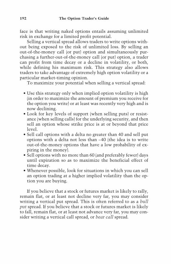
face is that writing naked options entails assuming unlimitedrisk in exchange for a limited profit potential.
Selling a vertical spread allows traders to write options with-out being exposed to the risk of unlimited loss. By selling anout-of-the-money call (or put) option and simultaneously pur-chasing a further-out-of-the-money call (or put) option, a tradercan profit from time decay or a decline in volatility, or both,while defining his maximum risk. This strategy also allowstraders to take advantage of extremely high option volatility or aparticular market-timing opinion.
To maximize your potential when selling a vertical spread:
• Use this strategy only when implied option volatility is high(in order to maximize the amount of premium you receive forthe option you write) or at least was recently very high and isnow declining.
• Look for key levels of support (when selling puts) or resist-ance (when selling calls) for the underlying security, and thensell an option whose strike price is at or beyond that pricelevel.
• Sell call options with a delta no greater than 40 and sell putoptions with a delta not less than –40 (the idea is to writeout-of-the-money options that have a low probability of ex-piring in the money).
• Sell options with no more than 60 (and preferably fewer) daysuntil expiration so as to maximize the beneficial effect oftime decay.
• Whenever possible, look for situations in which you can sellan option trading at a higher implied volatility than the op-tion you are buying.
If you believe that a stock or futures market is likely to rally,remain flat, or at least not decline very far, you may considerwriting a vertical put spread. This is often referred to as a bullput spread. If you believe that a stock or futures market is likelyto fall, remain flat, or at least not advance very far, you may con-sider writing a vertical call spread, or bear call spread.
192 The Option Trader’s Guide

The key to properly employing the “sell a verticalspread” strategy is finding situations in which the im-plied option volatility is high enough to allow you to re-ceive enough premium to justify entering this trade withits limited profit potential.
Writing options when implied volatility is high allows you towrite expensive options. This is a requirement when selling ver-tical spreads because it allows you to maximize the amount ofpremium you receive when entering the trade. Writing optionswhen option volatility is high also gives you the opportunity toprofit should option volatility decline in the near future.
Option writing can also be used in place of option buying totake advantage of a market-timing call if implied volatility isvery high. Naïve traders often make the mistake of buying op-tions when implied volatility is high. This stacks the deckagainst them by causing them to buy expensive options. The im-plication of buying expensive options is that the underlying se-curity must move that much further to compensate for theadditional time decay. A subsequent decline in volatility alsoserves to reduce the price of the option purchased. These factorscan present huge obstacles for a trader to overcome.
If you believe that the underlying is likely to move stronglyin a particular direction but implied volatility is high, you cansell a vertical spread on the other side of the market to profit ifthe expected price move occurs (by selling put spreads if you ex-pect the underlying to rise or selling call spreads if you expectthe underlying to fall). This is where you need to apply whatevermarket-timing method you prefer to indicate that a rise or fall inprice is likely. This part of the analysis is based on whatevertiming technique a trader decides to use.
There are several key factors to notice in Figures 16.1 and16.2 and Table 16.1.
• In Figure 16.1 you can see that IBM is attempting to establisha support level at 80.06.
Sell a Vertical Spread 193

• In Figure 16.2 the relative volatility rank for IBM options is10, the highest decile. This is an objective measure indicatingthat the options for this stock are currently expensive andthat this may be a good time to write options on the stock.
• In Table 16.1 the option we are looking to write (the Febru-
194 The Option Trader’s Guide
Figure 16.1 IBM – A support level forms at 80.06.
24-Month Relative Volatility Rank = 1054.98
52.48
49.98
47.48
44.98
42.48
39.98
37.48
34.98
32.48
29.98981229 990428 990827 991229 428 829 1228
Figure 16.2 IBM Relative Volatility Rank is 10.
13490
12576
11662
10748
9834
8920
8006804 828 920 1016 1108 1201 1228

ary 80 put) has 49 days left until expiration and a delta of –33.In other words, when we entered the trade there was a 67%probability that the option written would expire worthless.These are both within our guidelines (not more than 60 daysuntil expiration and a delta of 40 or less for the option wewrite) for selling vertical spreads.
The graph in Figure 16.3 shows risk curves for five dates lead-ing up to option expiration. With IBM trading at 85.25, we cansell 6 February 80 put options at a price of 4.62 ($462.50 per op-tion) and simultaneously purchase 6 February 75 put options at
Sell a Vertical Spread 195
Table 16.1 IBM Put Delta Not Less Than –40
Puts
JAN FEB APR JUL21 49 113 204
Delta –9 –14 –18 –20Bid 1.12 2.06 3.62 4.62
70Asked 1.50 2.31 3.87 5.12Imp. V. 83.91 67.38 57.77 50.59
Delta –19 –22 –26 –26Bid 2.00 3.12 4.87 6.12
75Asked 2.25 3.37 5.37 6.75Imp. V. 77.83 63.65 55.61 49.34
Delta –31 –33 –33 –33Bid 3.00 4.62 6.50 8.12
80Asked 3.38 5.12 7.12 8.75Imp. V. 69.69 61.61 53.45 48.70
Delta –45 –43 –41 –39Bid 5.12 6.50 8.62 10.37
85Asked 5.75 7.12 9.25 11.00Imp. V. 69.81 58.18 51.79 47.84
Delta –58 –54 –49 –45Bid 7.75 9.12 11.12 13.00
90Asked 8.38 9.75 11.75 13.62Imp. V. 66.08 56.22 50.13 47.27
Delta –70 –64 –57 –51Bid 11.12 12.50 14.25 15.87
95Asked 11.75 13.12 14.87 16.50Imp. V. 63.15 56.27 49.84 46.59

a price of 3.37 ($337.50 per option). Our maximum profit poten-tial is equal to the amount of the credit we receive when weenter the trade, which is $725 (1.25 points × $100 × 6 contracts).Our maximum risk of $1875 would occur if we were still hold-ing this position at option expiration and IBM was then tradingat 75 (i.e., the lower strike price) or lower.
Following the guidelines set out earlier for this strategy:
• We identified a market with high option volatility.• We sold a put option with a delta between 0 and –40 (the Feb-
ruary 80 put had a delta of –33).• We sold a put option with less than 60 days until expiration
(49 days in this case).• We sold an option with a higher implied volatility than the
option we bought.
Every option strategy offers some tradeoff. We can accuratelystate that there is a 68% probability that IBM will be above ourbreak-even price of 78.82 at option expiration. As mentioned inChapter 1, however, in order to properly assess our risk we mustalso look at what could happen to this position before expiration.As you can see, the danger of experiencing our maximum poten-
196 The Option Trader’s Guide
1125
562
0
–563
–1125
–1688
–225162.25 71.94 78.56 85.25 91.94 98.56 105.225
Date: 2/16/01 Profit/Loss: –5 Underlying: 78.82 Above: 68% Below: 32% % Move Required: –7.1%
Figure 16.3 Risk curves for IBM short vertical spread.

tial loss before expiration is low. However, one thing to considerwhen writing options is that profit potential is limited. In thisexample, our maximum profit potential is $725 while our maxi-mum risk is 2.5 times as great ($1875). In this case, the goodnews is that we have a 68% probability of making money. Thebad news is that we have a reward-to-risk ratio of only 1:2.5.
Based on these observations we recognize that if we were tolet this trade experience the maximum potential loss, it wouldtake three subsequent profitable trades just like it to offset theloss on this trade. Because our reward-to-risk ratio is 1:2.5, wemust do whatever we can to make certain that this trade neverreaches its maximum loss potential.
Position Taken
Sell 6 February 80 puts at 4.62.Sell 6 February 75 puts at 3.37.
Maximum profit $725Maximum risk –$1875Probability of profit 68%Current underlying price 85.25Break-even price at expiration 78.82
Position management is very important for option tradingsuccess. Our biggest concern with this particular trade is that wehave a maximum risk of $1875 but a maximum profit potentialof only $725. As a result, our biggest priority in managing thistrade is not to allow a large loss to occur that could take manysubsequent trades from which to recover.
In this case we will establish our stop-loss criteria first. Toreduce our risk-to-reward ratio from 1:2.5 to 1:1, we simply de-cide to exit this trade if it reaches an open loss of $725. If this oc-curs, we will exit the position, cut our loss, and move on. By sodoing, only one such similarly profitable trade would be requiredto recoup our loss.
To determine when we might need to exit this trade to cutour loss, we first look at the risk curves and determine approxi-mately how far the stock must move to generate a loss equal to
Sell a Vertical Spread 197
TEAMFLY
Team-Fly®

our maximum profit potential. By examining the risk curve forJanuary 5 (one week after the trade is entered), we find that thetrade would generate a loss of approximately $725 if IBM fell to77.50 by January 5. We then look at the bar chart for the under-lying security itself. What we want to see is some easily identi-fiable and meaningful support level above this price (for a call, orbelow this price if we are selling puts). In other words, for ourtrade to be stopped out, the underlying security must take out ameaningful support or resistance level rather than just experi-encing a random pullback in price.
Looking again at the bar chart for IBM in Figure 16.1, we seea support level at 80.06. So this trade fulfills the requirement justdiscussed. In other words, for our stop-loss level of 77.50 to bereached, IBM must first take out the support level at 80.06. In themeantime, as long as this support level holds, our trade will startto show a profit. For taking a profit we will use a simple tech-nique. We will take our profit if we reach 80% of the maximumprofit potential for this trade. The maximum profit potential is$725, so if we have an open profit of $580 or more, we will sim-ply take our money and run. This can happen in one of three ways:
1. A rise in the price of IBM stock2. A sharp decline in volatility3. The passage of time
If one or more of these factors combine to give us 80% of ourprofit potential, we will take our profit and move on at that pointrather than holding out for the last dollar and giving IBM thechance to fall back and jeopardize our profit. In summary, IBMmust decline below 77.50 for our stop-loss to be triggered. Anytype of market action other than an immediate price declineleaves us with a high probability of making money on this trade.
To give yourself the best chance of success in trading creditspreads:
• Look at a risk curve as of option expiration to determine yourmaximum profit potential.
• Look at risk curves before option expiration to see how farthe underlying must go against you to trigger a loss equal to
198 The Option Trader’s Guide

(or at most up to 20% more than) your maximum profitpotential.
• Look at a daily bar chart. Ideally there should be a major sup-port level (if selling puts, or a major resistance level if sellingcalls) between the current price of the underlying and thehypothetical stop-loss point identified in Step 2).
The bottom line is this: You don’t want to risk much morethan your maximum profit potential on the trade. In addition,you want to see a situation in which the underlying must firsttake out a major support or resistance level before it can reachyour stop-loss point.
Position Management
Stop-loss:
• Close trade if loss reaches –$725 (maximum profit times 1).• Alternatively, we could close the trade if IBM drops below
80.06, taking out the latest level of support.
Profit-taking: Close trade if profit reaches $580 (80% of maxi-mum profit).
As we had hoped, IBM rallied after the trade was entered,thus resulting in declining put option prices. As you can see inFigure 16.4, within three weeks IBM rallied sharply and our ini-tial profit target of $580 was exceeded on January 18. Table 16.2shows the net result of this trade.
This example illustrates an important point when writingoptions: You generally should not hold out for the last dollar.
To understand this concept, consider the change in the re-ward-to-risk ratio since the trade was first entered. We had al-ready achieved $600 of our maximum $725 profit potential. As aresult, we had only another $125 of profit potential remaining.Thus, our reward-to-risk ratio had shifted from $725 potentialreward versus $1825 potential risk to $125 potential reward
Sell a Vertical Spread 199

versus $2375 potential risk. In other words, if we continued tohold this trade, we would be risking $2375 to make another$125. At this point the potential reward no longer justifies as-suming the potential risk.
Trade Result
Profit target was reached on January 18.Profit = $600
KEY POINT
When writing options, do not hold out for the last dollar.
200 The Option Trader’s Guide
12218
11516
10814
10112
9410
8708
8006928 1023 1114 1211 10105 10201 10227
Figure 16.4 IBM rallies, profit taken on January 18.
Table 16.2 IBM Bull Put Spread Result
Long/Short Quantity Type Price In Last Price $ + /–
Short 6 February 80 puts 4.62 0.50 +$2475Long 6 February 75 puts 3.37 0.25 –$1875

Chapter 17
SELL A NAKED PUT
201
PURPOSE: To use high option volatility to accumulatestock below current market prices.
Key Factors
1. Extremely high implied volatility exists (the higher, thebetter).
2. There is an identifiable support level.3. You want to own the underlying security.
Selling a naked put is a highly specialized strategy that mosttraders will never use and that quite frankly, many traders nevershould use. It involves nothing more than writing a naked putoption on a given underlying security. Once this trade is entered,one of three outcomes will occur:
1. The stock will remain above the strike price of the put optionand the option will expire worthless. In this case the writer ofthe option keeps the entire premium he or she originally col-lected when the option was written.
2. The price of the stock will fall below the strike price of theoption written, the option will be exercised, and the writer ofthe option will be assigned (i.e., required to purchase 100shares of stock at the strike price).
3. The writer of the put option will buy back the option beforeoutcome 1 or 2 occurs.

This strategy is used primarily by sophisticated investors whoare interested in accumulating shares of stock in a particularcompany but who for one reason or another are not willing tocommit to buying the shares at the moment. It is best suited forvalue investors, who typically accumulate a position of mean-ingful size in a stock after the stock declines in price and arewilling to hold the position for a reasonably long period. It is illsuited to short-term traders or momentum investors, who gen-erally attempt to buy high and sell higher.
The most important consideration when selling a naked putis whether you want to own the stock. If the answer is no, or ifyou are not really sure, you should not use this strategy. To un-derstand why, let’s consider the primary benefit of this strategyas well as the worst-case scenario. Investors who use this strat-egy generally do so in an effort to acquire stock at a price belowthe current market price. Here is how that happens.
Say a stock is trading at a price of $85 per share. At the sametime the 80 strike price put option is trading at a price of $3.You could buy the stock at $85 per share or you could write aput option with a strike price of 80 and collect a premium of 3points (or $300). If you buy 100 shares of stock at $85 per shareand it declines to $77 per share, you will lose $800. If you hadwritten a put option at a strike price of 80 for 3 points and thestock declines to $77 per share, you would be at break-even. Inother words, if the stock is put to you, your effective buy priceis $77 per share (equal to the strike price minus the premiumcollected, or 80 minus 3). This is the benefit of writing nakedputs. The disadvantages are these:
• If the stock rallies sharply, you will not participate in thatrally beyond the option premium you collected.
• If the stock falls sharply, you still have significant downsiderisk.
To maximize your potential when selling a naked put:
• Use this strategy only after you have analyzed the prospectsfor the underlying company and have consciously decidedthat you are definitely willing to buy the stock.
202 The Option Trader’s Guide

• Use this strategy only when implied option volatility is high(to maximize the amount of premium you receive for the op-tion you write).
• Look for a key level of support for the underlying securityand then sell an option whose strike price is close to or belowthat price level.
• Sell put options with a delta between 0 and –50 (in otherwords, write out-of-the-money options to put time decay toyour advantage).
• Sell options with no more than 60 days (and preferably fewer)until expiration (also to maximize the beneficial effect oftime decay).
The key to employing the “sell a naked put” strategy cor-rectly is to find a stock that you are willing to buy andwhose options are presently trading at extremely highvolatility levels.
In Figure 17.1 you can see that after a rally, IBM has pulledback toward its recent support level of 80.06. Figure 17.2 shows
Sell a Naked Put 203
Figure 17.1 IBM – A support level forms at 80.06.
11864
11221
10578
9935
9292
8649
80061121 1208 1229 10119 10207 10228 10319

that implied volatility for IBM options is extremely high. For aninvestor who is willing to buy IBM stock, this represents a goodsetup for writing a naked put option. In Table 17.1, you can seethat the April 85 put can be written for a premium of 3.60 points,or $360 per contract.
To write one IBM April 85 put with IBM stock trading at92.56, a trader must meet an initial margin requirement of$1095, as shown below. However, it is important to understandthat this margin requirement can rise if the price of the stock de-clines, and that ultimately the writer of the 85 put option may berequired to buy 100 shares of IBM at a price of $85 a share, or$8500.
Initial margin requirement:
(((Stock price × 20%) – (stock price – strike price))× 100)(((92.56 × .20) – (92.56 – 85)) × 100)
((18.51 – 7.56) × 100) = 10.95, or $1095
The risk curve graph in Figure 17.3 depicts risk curves forthree dates leading up to option expiration. With IBM tradingat 92.56, we sold 1 April 85 put at a price of 3.60 ($360). Our
204 The Option Trader’s Guide
24-Month Relative Volatility Rank = 10
54.98
52.48
49.98
47.48
44.98
42.48
39.98
37.48
34.98
32.48
29.98
990405 990730 991126 327 724 1120 10319
Figure 17.2 IBM volatility rank is a 10.

Sell a Naked Put 205
Table 17.1 IBM Put Delta Not Less Than –50
Puts
APR MAY JUL OCT32 60 123 214
Delta –4 –7 –12 –14Bid 1.10 1.70 3.00 4.0070Asked 1.35 1.95 3.30 4.40Imp. V. 83.04 69.73 60.84 53.50
Delta –9 –12 –17 –19Bid 1.60 2.45 4.00 5.2075Asked 1.85 2.75 4.30 5.60Imp. V. 76.44 66.19 58.16 51.74
Delta –17 –20 –24 –24Bid 2.40 3.40 5.30 6.6080Asked 2.70 3.70 5.70 7.10Imp. V. 71.52 62.02 56.29 50.18
Delta –27 –29 –30 –30Bid 3.60 4.70 6.80 8.4085Asked 3.90 5.00 7.30 8.90Imp. V. 67.20 58.45 54.00 49.13
Delta –39 –39 –38 –36Bid 5.30 6.60 8.60 10.5090Asked 5.70 7.00 9.10 11.00Imp. V. 64.09 56.93 51.54 48.20
512
0
–511
–102372.60 79.25 85.94 92.56 99.25 105.94 112.56
Date: 4/20/01 Profit/Loss: 2 Underlying: 81.48 Above: 84% Below: 16% % Move Required: –11.9%
Figure 17.3 Risk curves for IBM short put.

maximum profit potential is equal to the amount of the creditwe receive when we enter the trade, which is $360. If we holdthis option until April expiration, one of two things willhappen:
1. The option will expire out of the money and we will keep the$360 premium.
2. The option will expire in the money and we will buy 100shares of IBM stock at $85 a share.
Following the guidelines set out earlier for this strategy:
1. We identified a stock in which we wish to accumulate aposition (IBM).
2. We waited until the option volatility for that stock was ex-tremely high (relative volatility rank of "10").
3. We sold a put option with a delta between 0 and –50 (theApril 85 put had a delta of –27).
4. We sold a put option with less than 60 days until expiration(32 days in this case).
Looking only at the risk curve at expiration we can accu-rately state that there is an 84% probability that IBM will beabove our break-even price of 81.40 at option expiration.
Position Taken
Sell 1 April 85 put at 3.60.
Maximum profit $360Maximum risk UnlimitedProbability of profit 84%Current underlying price 92.56Break-even price at expiration 81.40
Our initial position-management criteria for this trade arefairly straightforward. We will either collect the premium if the
206 The Option Trader’s Guide

stock stays above the option’s strike price or buy the stock if itfalls below the strike price.
Two different worst-case scenarios are associated withselling a naked put. The first occurs if the stock goes wayup; the second occurs if the stock goes way down.
If the stock rallies, the good news is that we stand to makethe equivalent of 3.60 points by virtue of having written a putoption. If the stock advances more than that, we will gain no ad-ditional profit. For example, if the stock rallies 10 points, wemight end up wishing that we had simply bought the stock.However, by writing a naked put we made a conscious decisionto try to buy the stock at a lower price, and for now we must besatisfied to collect the option premium for the put we wrote. Ifwe want, we can always write another put and start the sameprocess again.
If the stock falls, the good news is that we will have the op-portunity to buy it at a lower price than if we had bought thestock rather than writing the put option. The danger is that thestock will fall significantly below the strike price of the put op-tion we wrote. Should this occur and the stock be put to us, wemay quickly be saddled with a large open loss on our stock posi-tion. When a stock is trading at 92.56, having the opportunity tobuy it a price of 81.40 sounds very enticing. However, if the un-derlying company comes out with a surprisingly bad earnings an-nouncement and the stock gaps down 30 points overnight, theprospect of buying the stock at 81.40 no longer sounds like sucha great proposition. Unfortunately, if you are short a naked put,you will have no choice but to either buy back the put—mostlikely at a significant loss—or buy the stock at the strike priceand hope that it does not decline much more before rising backinto profitable territory. The prospect of facing this very situa-tion is why this strategy is best suited for investors who are al-ready comfortable accumulating and holding a position in astock for a reasonable length of time. It also illustrates the needfor thorough investigation of the prospects for the underlyingcompany before writing a naked put.
Sell a Naked Put 207
TEAMFLY
Team-Fly®

In this example we have decided that we are willing to buyIBM stock if it is put to us. Therefore, our position-managementrules are fairly simple: We will hold the option until expirationand either collect $360 in premium or buy the stock at an effec-tive price of 81.40. In light of the worst-case scenario on thedownside, we must also establish some criteria for exiting thestock position if it continues to decline.
One Method for Managing Stock Position If Assigned
There are any number of ways to manage a stock position onceentered. However, our specific concern in this case is decidingwhat we will do if the stock is put to us and its price continuesto decline. One method worth considering is to risk the amountyou saved. For example, in this trade we could have bought IBMstock outright at a price of 92.56 per share. Instead, we wrote the85 put and collected 3.60 points of premium. As a result our ef-fective purchase price if the stock is put to us is 81.40 (85 – 3.60).If the stock had stopped declining at that price, we would havesaved ourselves 11.16 per share compared to buying the stockoutright when it was at 92.56. Some traders might simply ear-mark this stock position as a long-term holding. Others mightlook at recent support levels and attempt to identity a good placeto stop themselves out if the stock continues to decline. Oneother alternative is to use the amount that you saved by initiallywriting the naked put as a stop-loss value. Let’s see how thatwould work in this example.
If the stock declines and we buy it at an effective price of81.40, saving 11.16 per share, we can then place a stop-loss orderto sell the stock if it falls to 70.24. This value is arrived at by sub-tracting the amount we saved by writing the option initially(11.16 points) from our effective purchase price of 81.40. The badnews in using this method is that although we saved 11.16points compared to buying the stock at 92.56, if the stop-lossprice is hit, we will still lose money on the trade ($1116). Thegood news is that we will still come out ahead of where wewould have been if we had bought the stock at 92.56 initially.
208 The Option Trader’s Guide

Position Management
• Hold the position until the option expires or the stock is putto us at $85 a share.
• If the stock is put to us at effective price of 81.40 (85 – 3.60),we will have saved 11.16 a share (92.56 – 81.40). We will riskthis amount on the trade and place a stop at 70.24.
Trade Result
Between the time this trade was entered and April option expi-ration, the price of IBM rallied sharply. As a result, the April 85put option expired worthless (Figure 17.4).
Profit = $360
Sell a Naked Put 209
11864
11221
10578
9935
9292
8649
80061116 1212 10105 10202 10305 10327 10420
Figure 17.4 IBM rallies, put option expires worthless.


Chapter 18
WRITE A COVERED CALL
211
PURPOSE: To use time decay or high option volatility tohedge and/or generate income from an existing position.
Key Factors
1. You have some reason to expect the underlying to pause.2. Option volatility is high.3. You can take advantage of time decay by selling out-of-the-
money options.
Options offer traders a number of unique opportunities. One op-portunity they offer—particularly to longer-term investors—isthe ability to hedge existing positions in an underlying security.If a trader is holding a position in a particular stock or futuresmarket and wants to hedge that position, options are often theeasiest and most effective alternative for achieving this objec-tive. The most popular and commonly used hedging strategy isknown as covered call writing. A covered call write involveswriting a call option against a long position in the underlyingsecurity.
Although it is a popular strategy, covered call writing is prob-ably the most commonly misused option-trading strategy. Mosttraders never consider writing covered calls until it is suggestedto them by a broker. Once they do, they rarely stop to consider

the reward and risk ramifications. At best, writing a covered callallows a trader to generate income from an existing position andto obtain some downside protection. At worst, this strategy lim-its your upside potential and provides only a limited amount ofdownside protection.
There are a number of different ways to use this strategy. Forinstance, some traders buy a stock they consider oversold and si-multaneously write a call option against that position. This isgenerally referred to as a buy-write and is employed by an in-vestor who is focused on total return (gain or loss on stock plusoption premium collected). The method presented in this chap-ter differs slightly from that approach in that it involves writingcall options against stocks (or futures contracts) that are alreadyheld, based on a given set of circumstances that we will discuss.
Covered calls should be written only when implied optionvolatility is high. This allows you to sell expensive options andto maximize the amount of premium you collect. Remember,writing a covered call affords you only a limited amount ofdownside protection and limits the amount of your upside po-tential. The higher the implied volatility, the more time pre-mium an option writer can collect; therefore, the more downsideprotection he or she is afforded. Because of these factors youshould only use this strategy when you can obtain a substantialamount of premium.
Covered call writing is not a market-timing strategy per se. Itsimply gives an investor the opportunity to take advantage ofhigh option volatility and time decay. The way to take maxi-mum advantage of time decay is to write out-of-the-money calloptions (which will likely expire worthless) when impliedvolatility is high.
The example trade in this chapter involves the stock of Com-puter Associates (symbol: CA).
1. In the graph in Figure 18.1 you can see that CA stock rallied91% in just 11 trading days and then fell back below a long-term resistance level.
2. Figure 18.2 shows that the relative volatility rank is 10, indi-cating that CA options are expensive, thus signaling a favor-able time to write options on this security.
212 The Option Trader’s Guide
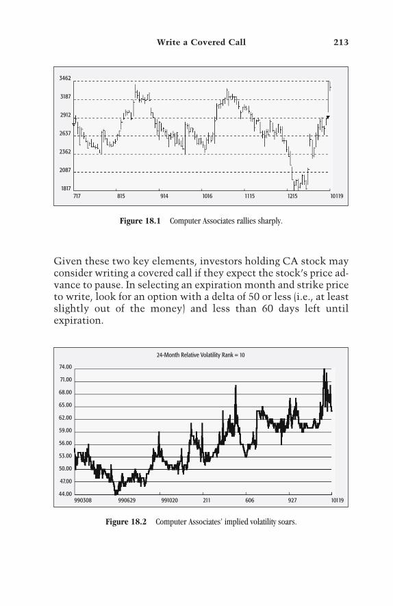
Given these two key elements, investors holding CA stock mayconsider writing a covered call if they expect the stock’s price ad-vance to pause. In selecting an expiration month and strike priceto write, look for an option with a delta of 50 or less (i.e., at leastslightly out of the money) and less than 60 days left untilexpiration.
Write a Covered Call 213
3462
3187
2912
2637
2362
2087
1817717 815 914 1016 1115 1215 10119
Figure 18.1 Computer Associates rallies sharply.
24-Month Relative Volatility Rank = 10
74.00
71.00
68.00
65.00
62.00
59.00
56.00
53.00
50.00
47.00
44.00990308 990629 991020 211 606 927 10119
Figure 18.2 Computer Associates’ implied volatility soars.
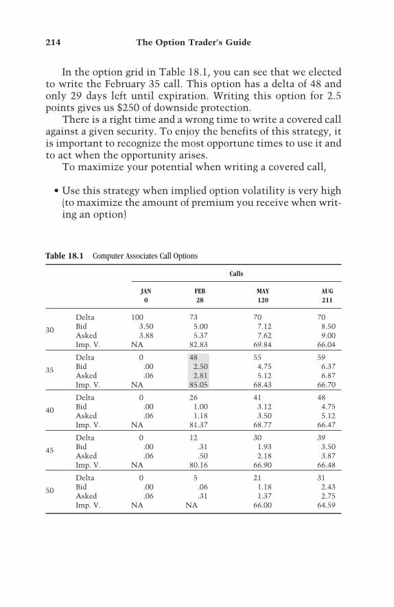
Table 18.1 Computer Associates Call Options
Calls
JAN FEB MAY AUG0 28 120 211
Delta 100 73 70 70Bid 3.50 5.00 7.12 8.5030Asked 3.88 5.37 7.62 9.00Imp. V. NA 82.83 69.84 66.04
Delta 0 48 55 59Bid .00 2.50 4.75 6.3735Asked .06 2.81 5.12 6.87Imp. V. NA 85.05 68.43 66.70
Delta 0 26 41 48Bid .00 1.00 3.12 4.7540Asked .06 1.18 3.50 5.12Imp. V. NA 81.37 68.77 66.47
Delta 0 12 30 39Bid .00 .31 1.93 3.5045Asked .06 .50 2.18 3.87Imp. V. NA 80.16 66.90 66.48
Delta 0 5 21 31Bid .00 .06 1.18 2.4350Asked .06 .31 1.37 2.75Imp. V. NA NA 66.00 64.59
In the option grid in Table 18.1, you can see that we electedto write the February 35 call. This option has a delta of 48 andonly 29 days left until expiration. Writing this option for 2.5points gives us $250 of downside protection.
There is a right time and a wrong time to write a covered callagainst a given security. To enjoy the benefits of this strategy, itis important to recognize the most opportune times to use it andto act when the opportunity arises.
To maximize your potential when writing a covered call,
• Use this strategy when implied option volatility is very high(to maximize the amount of premium you receive when writ-ing an option)
214 The Option Trader’s Guide

• Sell call options with a delta no greater than 50 (i.e., sell anout-of-the-money call to maximize the beneficial effects oftime decay)
• Sell options with no more than 60 (and preferably fewer) daysuntil expiration
• Use this strategy after a security you are holding has experi-enced a significant rally and you expect it to consolidate ordecline in the near term
In sum, if a security you are holding has experienced a sharp ad-vance in price and implied volatility rises to a very high level,thus inflating the amount of premium available to option writ-ers, you may benefit from writing a covered call.
The graph in Figure 18.3 depicts risk curves for three datesleading up to option expiration. While holding long 100 shares ofCA, and with CA trading at 33.69, we sold one February 35 calloption at a price of 2.50 (thus collecting $250 in premium).
The advantage of making this trade is that the $250 we re-ceive for writing this option is ours to keep. As a result, thebreak-even point on our stock position (from this point forward)is reduced from 33.69 (if we were just holding the stock) to 31.39.
Write a Covered Call 215
503
84
–336
–75523.68 27.00 30.31 33.69 37.00 40.31 43.69
Date: 2/16/01 Profit/Loss: –1 Underlying: 31.19 Above: 68% Below: 32% % Move Required: –7.8%
Figure 18.3 Computer Associates covered call risk curves.

To put it another way, we have 7.8% of downside protection.When the option was written, the probability of CA trading at orabove this price at February option expiration was 65%. The dis-advantage of writing a covered call is that it limits upside poten-tial. If CA is trading above 35 at the time the February optionsexpire the most that we can make on this trade is $380, regard-less of how high the stock might rally.
You are limiting your upside potential while receiving only alimited amount of downside protection. This is an importantfactor that most traders never consider when writing coveredcalls.
Following the guidelines set out earlier for this strategy:
• We chose a stock with high option volatility (a relativevolatility rank of 10) that was overbought.
• We sold a call option with a delta of less than 50 (the Febru-ary 35 call has a delta of 48).
• We sold a call option with less than 60 days until expiration(the February options have 28 days left until expiration).
Position Taken
Long 100 shares of CASell 1 February 35 call at 2.50.
In deciding how to manage a covered call position, you mustaddress two risks:
1. The first risk is that the stock may fall by more than theamount received when the call option was written. Oncethat happens, the covered call provides no additional protec-tion, so the potential loss becomes unlimited. (Technically,the risk is not unlimited since the stock can only go to zero,but the point is that beyond a certain price, the call option of-fers no additional protection.)
2. The second risk is that the stock may rally sharply, causingthe option that we wrote to trade in the money. Once the op-tion trades in the money, there is a possibility that the holder
216 The Option Trader’s Guide

of the option may exercise the option and our stock will becalled away. If we do not want to give up our stock position,we must plan to buy back the call if the stock price rises.
Before writing a covered call, you must decide what you willdo if the stock drops sharply or rallies sharply. If the stock dropssharply, your choices are these:
• Sell the stock, buy back the call, and exit the trade com-pletely to avoid additional losses.
• Hold onto both positions and hope the stock bounces back.• Roll down. Rolling down involves buying back the call op-
tion written initially and selling a new call option with alower strike price. This is something of an advanced tech-nique and will not be covered in detail here.
If the stock rallies sharply, you may do one of three things:
1. Let the stock be called away.2. Buy back the call option you wrote (possibly at a higher price,
thus incurring a loss).3. Buy back the call option you wrote (possibly at a loss) and
sell another further-out-of-the-money call option.
There are no absolute right or wrong answers for these deci-sions. Deciding whether to buy back the call or to let the stockbe called away may depend on a number of factors. If you defi-nitely want to hold the stock, or if you have a large gain and donot want to sell the stock, thus realizing a taxable capital gain,you will buy back the call option, more than likely paying ahigher price than you sold it for originally. If you want, you canwrite another call with a higher strike price at that time. Al-though some traders like to think of covered call writing as “freemoney,” you are essentially trading upside potential for a lim-ited amount of downside protection. If the underlying securitystarts to rally and you buy back the call at a loss, the net effect isthat your position-protecting, income-producing hedge ends upgenerating a loss.
For this example, we chose to let the stock be called away if
Write a Covered Call 217
TEAMFLY
Team-Fly®

the stock rallied above 35 and the option was exercised againstus. On the downside, we entered a stop-loss to sell the stock at29. A drop in this price would require a drop back into the previ-ous trading range and would be a signal to us that the recentbreakout had failed. If our stop-loss price for the stock is hit, wewill simultaneously buy back the call option to avoid holding ashort naked call position. Remember that holding a naked shortcall exposes you to unlimited risk.
Position Management
Stop-loss: Sell the stock and buy back the call option if the stockdrops below 29.
Profit-taking: If the stock rises, hold until option expiration oruntil the stock is called away.
As shown in Figure 18.4, CA stock failed to follow through tothe upside and drifted sideways to slightly higher through Febru-ary option expiration. At the close of trading on option-expirationday, the stock was trading at 35.90. As a result, the 35 call was0.90 point in the money. If we did not buy this call back before
218 The Option Trader’s Guide
3900
3552
3204
2856
2508
2160
18121024 1109 1130 1219 10109 10130 10216
Figure 18.4 Computer Associates at February option expiration.

the close of trading, it would automatically be exercised by theOptions Clearing Corporation and our stock would be calledaway. If we had wanted to continue to hold the stock, we wouldhave to buy back the call before the close of trading on that day.
In this example, writing a covered call helped us achieve thebest of both worlds. The stock rose from 33.69 to 35.90, generat-ing a profit of $221. At the same time, the February 35 call lostall of its time premium and declined in price from 2.50 to 0.90 atexpiration, generating another profit of $160 to the writer of thisoption (Table 18.2).
The end result is that as of February option expiration wehave a profit of $380 and would still be holding our stock posi-tion if we bought back the call just before expiration. If we heldthe option through expiration, our stock position would becalled away because our short option is in the money, thus trig-gering automatic exercise.
Write a Covered Call 219
KEY POINT
Covered call writing should be considered only when implied volatility ishigh. Sell only out-of-the-money call options to maximize the effects of timedecay.
Trade Result
Option expired at 0.90 on February 16.Stock closed at 35.90.
Table 18.2 Computer Associates Covered Call Result
Long/Short Quantity Type Price In Last Price $ + /–
Long 100 Shares 33.69 35.90 +$221Short 1 February 35 call 2.50 0.90 +$160
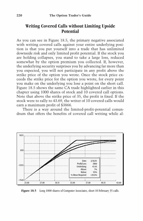
Writing Covered Calls without Limiting UpsidePotential
As you can see in Figure 18.5, the primary negative associatedwith writing covered calls against your entire underlying posi-tion is that you put yourself into a trade that has unlimiteddownside risk and only limited profit potential. If the stock youare holding collapses, you stand to take a large loss, reducedsomewhat by the option premium you collected. If, however,the underlying security surprises you by advancing far more thanyou expected, you will not participate in any profit above thestrike price of the option you wrote. Once the stock price ex-ceeds the strike price for the option you wrote, for every pointyou make on the underlying you lose a point on the short call.Figure 18.5 shows the same CA trade highlighted earlier in thischapter using 1000 shares of stock and 10 covered call options.Note that above the strike price of 35, the profit is fixed. If thestock were to rally to 43.69, the writer of 10 covered calls wouldearn a maximum profit of $3866.
There is a way around the limited-profit-potential conun-drum that offers the benefits of covered call writing while al-
220 The Option Trader’s Guide
5033
839
–3355
–754923.68 27.00 30.31 33.69 37.00 40.31 43.69
Date: 2/16/01 Profit/Loss: 3866 Underlying: 43.65 Above: 7% Below: 93% % Move Required: +29.6%
Figure 18.5 Long 1000 shares of Computer Associates, short 10 February 35 calls.

lowing you to participate in favorable movement by the under-lying: Simply avoid writing covered calls in a 1:1 ratio. In otherwords, if you are holding 1000 shares of stock, you might con-sider writing 8 call options (or any number less than 10) insteadof 10. By doing so, you still take in option premium, which offersyou some downside protection and the opportunity to earn extraincome. In addition, if the underlying security rallies sharply, al-though some of your position will likely be called away, you stillretain a position in the underlying security.
Figure 18.6 shows the same CA trade highlighted earlier inthis chapter using 1000 shares of stock, but only 8 covered-calloptions. Note that the profit on this trade continues to rise as thestock price advances. If the stock were to rally to 43.69, thewriter of 8 covered calls would have a profit of $5020, and thisprofit would continue to grow as the stock advances.
From the perspective of a long-term strategy, writing lessthan the full number of options possible against your underlyingposition offers an attractive reward-to-risk tradeoff.
Write a Covered Call 221
5033
894
–3573
–804023.68 27.00 30.31 33.69 37.00 40.31 43.69
Date: 2/16/01 Profit/Loss: 5020 Underlying: 43.65 Above: 7% Below: 93% % Move Required: +29.6%
Figure 18.6 Long 1000 shares of Computer Associates, short 8 February 35 calls.


Chapter 19
ENTER A BUTTERFLY SPREAD
223
PURPOSE: To take advantage of high volatility andtrading range conditions to collect option premium.
Key Factors
1. You have some reason to expect the underlying to stay in atrading range.
2. Option volatility is high (the higher, the better).3. Less than 60 days remain until expiration.4. You can enter the spread at a favorable price.
The butterfly spread strategy using calls involves buying acall option at one strike price, writing two calls at a higher strikeprice, and buying one more call at an even higher strike price.The butterfly spread strategy using puts involves buying a putoption at one strike, writing two puts at a lower strike, and buy-ing one more put at an even lower strike price. This trade is al-ways done in a ratio of 1:2:1. In other words, you may enter thespread in a ratio of 1:2:1, 2:4:2, 3:6:3, 5:10:5, 10:20:10, and so on.From a strictly mathematical viewpoint, the butterfly spread canoffer a very high probability of making money on any given trade.
A butterfly spread is a very specialized type of trade. Manytraders learn about this strategy, try it a time or two, fail to makemuch money or actually lose money, and never try it again. To

succeed with this strategy, you must understand the right cir-cumstances for using it and then act decisively when the oppor-tunity arises.
These are the key elements to look for when selecting but-terfly spreads:
• Choose an underlying security that is trading in a range withmeaningful support and resistance points. Once a butterflyspread is entered, the ideal scenario is for the underlying toremain relatively unchanged. Before entering a butterflyspread on a given security, look at a daily or weekly bar chartand see if you can easily identify meaningful support and re-sistance levels below and above the current price of the un-derlying. In other words, you want to find a security thatappears to be in a trading range. This clearly involves somesubjective analysis and there is of course no guarantee thatthe security will remain in a trading range. However, themain point is that if you find that the security you are con-sidering is trending strongly or has just broken out to a newhigh or low, it is probably a poor candidate for this strategy.
• Implied option volatility is high. When you are consideringa butterfly spread, option volatility should be as high as pos-sible. This strategy makes money from having the middlestrike price (i.e., the option you write) lose time premium. Inother words, the more time premium built into the price ofthe option you write, the greater your profit potential. There-fore, the way to maximize your profit potential is to focus onsecurities with high option volatility.
• No more than 60 days remain until option expiration. Bywriting options when volatility is high, we hope to profitfrom a decline in volatility. We also can add time decay toour arsenal by writing options that do not have much timeleft until expiration. Ideally, you will enter butterfly spreadsusing options with 30 days or less until expiration. As a ruleof thumb, you should not go out more than 60 days.
• Sell at-the-money or slightly out-of-the-money options. Thisis more of a guideline than a rule, but ideally you should lookto write an option that is at the money or one strike price outof the money. Writing an out-of-the-money option gives you
224 The Option Trader’s Guide
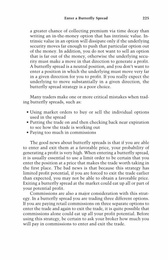
a greater chance of collecting premium via time decay thanwriting an in-the-money option that has intrinsic value. In-trinsic value in an option will dissipate only if the underlyingsecurity moves far enough to push that particular option outof the money. In addition, you do not want to sell an optionthat is far out of the money, otherwise the underlying secu-rity must make a move in that direction to generate a profit.A butterfly spread is a neutral position, and you don’t want toenter a position in which the underlying must move very farin a given direction for you to profit. If you really expect theunderlying to move substantially in a given direction, thebutterfly spread strategy is a poor choice.
Many traders make one or more critical mistakes when trad-ing butterfly spreads, such as:
• Using market orders to buy or sell the individual optionsused in the spread
• Putting the trade on and then checking back near expirationto see how the trade is working out
• Paying too much in commissions
The good news about butterfly spreads is that if you are ableto enter and exit them at a favorable price, your probability ofgenerating a profit is very high. When entering a butterfly spread,it is usually essential to use a limit order to be certain that youenter the position at a price that makes the trade worth taking inthe first place. The bad news is that because this strategy haslimited profit potential, if you are forced to exit the trade earlierthan expected, you may not be able to obtain a favorable price.Exiting a butterfly spread at the market could eat up all or part ofyour potential profit.
Commissions are also a major consideration with this strat-egy. In a butterfly spread you are trading three different options.If you are paying retail commissions on three separate options toenter the trade and again to exit the trade, it is quite possible thatcommissions alone could eat up all your profit potential. Beforeusing this strategy, be certain to ask your broker how much youwill pay in commissions to enter and exit the trade.
Enter a Butterfly Spread 225

In Figure 19.1 you can see that as of January 5, impliedvolatility on Intel options was extremely high. In Figure 19.2you can identify support and resistance levels for the price ofIntel stock at 29.81 and 47.15, respectively. This suggests thatIntel may be a good candidate for a butterfly spread. With Inteltrading at 32.06, we see in Table 19.1 that we can sell the at-the-money 32.5 February option as the middle option in a butterflyspread. We want to buy 1 February 27.5 call and 1 February 37.5call for every 2 February 32.5 calls we write. If we can enter thisspread at current market prices, we will enter the trade at a netdelta of 0, indicating a trade that is almost exactly neutral. Themarket prices for the 27.5 call, the 32.5 call, and the 37.5 call are5.75, 3.06, and 1.19, respectively. On a 1:2:1 spread, the net debit(i.e., the amount we would pay to enter the spread) would be(5.75 – (3.06 × 2) – 1.19), or 0.8125, or $81.25. If we want to do a5:10:5 butterfly spread at this price, we would need to place thefollowing order with the broker:
I want to enter a spread order as follows: This is a dayorder [Do not place open orders to enter a butterflyspread. The underlying might make a huge move by to-morrow, and a spread that is neutral today may be far
226 The Option Trader’s Guide
Figure 19.1 Intel option volatility is at the high end of its historic range.
24-Month Relative Volatility Rank = 10
73.32
69.92
66.52
63.12
59.72
56.32
52.92
49.52
46.12
42.72
39.32990310 990629 991018 207 529 915 10105

Enter a Butterfly Spread 227
6449
5871
5293
4715
4137
3559
2981929 1013 1031 1115 1201 1219 10105
Figure 19.2 Intel has identifiable support (29.81) and resistance (47.15) levels.
Table 19.1 Establish a Butterfly Spread Using Intel Calls
Calls
JAN FEB APR JUL14 42 106 197
Price 7.38 8.00 9.12 10.3825
Delta 95 88 81 79Imp. V. 100.05 78.05 70.12 67.31
Price 5.25 5.75 7.12 8.7527.5Delta 85 78 74 73Imp. V. 87.81 73.15 69.62 64.66
Price 3.25 4.38 5.88 7.3830Delta 69 66 65 66Imp. V. 83.26 73.40 68.58 63.40
Price 1.88 3.06 4.75 6.1232.5Delta 50 53 57 60Imp. V. 80.37 71.80 67.20 62.45
Price 1.00 2.00 3.50 5.0035Delta 32 41 49 53Imp. V. 78.83 71.23 66.59 61.88
Price .44 1.19 2.75 4.0037.5Delta 18 30 41 47Imp. V. 80.27 67.73 65.62 61.11
TEAMFLY
Team-Fly®

in the money or out of the money tomorrow, leavingyou in a very unfavorable trade.] Buy 1 February 27.5 call.Buy 1 February 37.5 call. Sell 2 February 32.5 calls. Buythis spread five times at a limit price of 0.8125 perspread.
Once this order is placed, it will either be filled at a net debit of$406 ($81.25 × 5) or less or you will enter no position at all (seeChapter 20 for more information on placing option-tradingorders).
If you are planning to trade butterfly spreads it is a good ideato get in touch with your broker beforehand to verify the appro-priate procedure for entering this type of spread order and thecommissions involved. If your broker does not know what a but-terfly spread is, get another broker for your option trading.
The graph in Figure 19.3 depicts risk curves for five datesleading up to option expiration. With Intel trading at 32.06, wepurchased 5 February 27.5 calls at 5.75, sold 10 February 32.5calls at 3.06, and bought 5 February 37.5 calls at 1.19. The totaldollar risk associated with this trade is equal to the amount ofpremium paid to buy the options, or $406 in this case.
228 The Option Trader’s Guide
2003
1113
223
–66822.06 25.38 28.75 32.06 35.38 38.75 42.06
Date: 2/16/01 Profit/Loss: –2 Underlying: 36.66 Above: 24% Below: 76% % Move Required: +14.6%
Figure 19.3 Intel butterfly spread risk curves.

The risk curve lines in the graph in Figure 19.3 clearly depictthe positive effect of time decay that will occur if Intel stayswithin its current range. There is a tradeoff involved: Initiallythe range of profitability is quite wide, but as expiration drawscloser, the goods news is that the maximum potential profitrises each week. The bad news is that the range of underlyingprices that will result in a profit grows narrower each week. Thisis simply a function of time decay.
Many traders look at the risk curves for a butterfly spreadand become mesmerized by the maximum potentialprofit at expiration. This is a mistake.
This profit will be obtained only if the underlying closes onoption-expiration day at exactly the middle strike price. Theodds of this happening are extremely slim and not worth playingfor.
As indicated on the graph (Figure 19.3), if we were to holdthis position until option expiration, our break-even prices are28.30 on the downside and 36.70 on the upside. If we are stillholding this position near expiration and Intel is not trading out-side of that range, this trade should show a profit. When thetrade was entered, there was a 25% probability that Intel wouldbe below 28.30 at expiration and a 27% probability that Intelwould be above 36.70. Statistically, there is a 50% probabilitythat Intel would be between the two break-even points of 28.30and 36.70 at option expiration.
The primary risk involved with the butterfly spread is thatthe underlying security will make a significant price move be-fore option expiration, thus leaving it outside your break-evenpoints.
Position Taken
Buy 5 February 27.5 calls at 5.75.Sell 10 February 32.5 calls at 3.06.Buy 5 February 37.5 calls at 1.19.
Enter a Butterfly Spread 229

Maximum risk –$406Net delta 10Days to expiration 42Probability of profit 47%Current underlying price 32.06Break-even price at expiration Above 28.30 and below 36.70
In theory the maximum risk on this trade is $406. In theworst-case scenario (i.e., if Intel rallies or declines sharply and istrading below 27.5 or above 37.5 at expiration), we can in theoryhold this trade until expiration and lose no more than thatamount. However, with a butterfly spread it can be a little morecomplicated than that. If Intel is trading below 27.5 at expiration,all the options in our spread will expire worthless. No follow-upaction is needed, and we would take a loss of $406.
At any price above 27.5, however, follow-up action may beneeded before expiration. To understand why follow-up actionmay be needed, consider the following scenarios:
• If we hold this trade through expiration and Intel closes at 30,our 5 27.5 calls will automatically be exercised and, come thefollowing Monday morning, we will be long 500 shares ofIntel stock at a cost of $13,750 (5 calls × 27.5 × $100).
• If we hold this trade through expiration and Intel closes at 35,our 5 27.5 calls will automatically be exercised, as will our 10short 32.5 calls. Come the following Monday morning, wewill be short 500 shares of Intel stock with the appropriatemargin requirement due to maintain this position.
• If we hold this trade through expiration and Intel closes at 40,all our options from this trade will automatically be exer-cised and will offset each other, leaving us with no positionin the underlying.
The real danger here occurs about 10 minutes before the closeof trading on option-expiration day. If the stock is trading at 27.25just before expiration, a trader might assume that he does notneed to be concerned about any exercise or assignment compli-cations. However, if the stock rallies 1.00 in the final 10 minutes
230 The Option Trader’s Guide

of trading and closes at 28.25, the trader will be assigned on the27.5 calls. The bottom line is that if we do not want to assume aposition in the underlying security, we must plan on exiting thistrade before expiration. And therein lies another complication.
Because we are buying and selling three different options, ifwe were to simply close each position at the market, chances arethat the bid-ask spreads would eat up much, if not all, our po-tential profit. Similarly, if we place a limit order to get out of thespread at a certain amount, there is a chance we might not getfilled at all. This potentially tricky situation is one of the reasonswe described butterfly spreads as a specialized strategy.
There are no magic formulas for determining when to exit abutterfly spread. What is important is to have a plan for exitingthe trade when you enter the trade. One useful rule of thumb isto plan to exit the trade before expiration at the first good oppor-tunity. We define a good opportunity as a situation in which theunderlying security is trading between our break-even points andvolatility has fallen enough, or time decay has worked enough inour favor, to generate an acceptable open profit. At that point wetake what profit we can from this trade and move on.
We will also set in place two other contingency plans:
1. If Intel falls in price and the amount of time premium in theFebruary 32.5 calls that we wrote drops to 0.25 or lower, wewill close the entire trade.
2. If Intel rallies in price and the amount of time premium inthe February 32.5 calls that we wrote falls to 0.125 points orless, we will exit the entire trade.
Contingency 1 is essentially a stop-loss measure. Althoughour risk is limited, if Intel falls far enough that our short optionhas almost no time premium left, it is basically a long shot to getback into our profitable range.
Contingency 2 is a measure designed to keep from getting as-signed on the short option.
Barring the occurrence of contingency 1 or 2, we will waitto exit this trade at the first good opportunity. Looking againat Figure 19.1, you will see that in the past two years option
Enter a Butterfly Spread 231

volatility for Intel has ranged from a high of 73 to a low of 39.Figure 19.4 shows the expected return for this trade a week be-fore expiration, depending on the level of volatility at that time.If the price of Intel is between the upper and lower strikes (27.5and 37.5), the lower the volatility, the higher the maximumprofit potential.
If Intel is unchanged a week before expiration and volatilityfalls to its previous low of 39, we would expect this trade toshow an open profit of approximately $1386. This possibility isshown by the uppermost line, which peaks in the middle of thegraph in Figure 19.4. Conversely, if Intel is unchanged a week be-fore expiration and volatility rises to its previous high of 73, wewould expect this trade to show an open profit of approximately$868. This possibility is shown by the bottom line, which peaksin the middle of the graph.
It would be extremely optimistic to assume that the stockwill be unchanged and that volatility will fall to its previouslow. Therefore, we decide arbitrarily that if we can close out theentire trade with a profit of $500 or more, we will do so whenthat opportunity arises.
232 The Option Trader’s Guide
1386
770
154
–46222.06 25.38 28.75 32.06 35.38 38.75 42.06
Date: 2/09/01 Profit/Loss: 1383 Underlying: 32.45 Above: 49% Below: 51% % Move Required: +0.6%
Figure 19.4 Intel butterfly spread risk curves for February 9, assuming different volatilitylevels.

Remember, the higher the profit you strive to attain, thelower the probability that you will attain it.
Position Management
Stop-loss:
• Close trade if price of February 32.5 call drops to 0.25 orlower.
• Close trade if time premium left in February 32.5 call dropsto 0.125.
Profit-taking: If the trade can be exited with a profit of $500 ormore before expiration, close the trade.
As you can see in Table 19.2, this trade worked out well,generating a profit of $778 as of February 9, which was one weekbefore option expiration. Figure 19.5 shows that Intel initiallyrallied above the upper strike price of 37.5. Had this rally con-tinued, we would have had to monitor the amount of time pre-mium in the February 32.5 call on a daily basis to avoid gettinginto a situation in which the option we had sold short might beexercised, thus throwing our trade out of whack. If we get as-signed on our short position, we would have to buy 1000 sharesof Intel at the market and deliver them at a price of 32.5 a share.We would still be left holding 5 27.5 calls and 5 37.5 calls. Thiswould be a far different situation than the one we intended to bein when we originally entered this butterfly spread.
Fortunately, that rally did not follow through and the stockfell back near the middle strike price, thus allowing time decay
Enter a Butterfly Spread 233
Table 19.2 Intel Butterfly Spread Results
Long/Short Quantity Type Price In Last Price $ + /–
Long 5 February 27.5 call 5.75 5.88 +$63Short 10 February 32.5 call 3.06 1.81 +$1248Long 5 February 37.5 call 1.19 .13 –$533

234 The Option Trader’s Guide
6215
5676
5137
4598
4059
3520
29811017 1102 1122 1212 10102 10123 10209
Figure 19.5 Intel stock price stays in a range.
24-Month Relative Volatility Rank = 10
73.32
69.92
66.52
63.12
59.72
56.32
52.92
49.52
46.12
42.72
39.32990209 990609 991011 209 609 1011 10209
Figure 19.6 Intel option volatility falls.
on the February 32.5 calls to begin working in our favor. Alsohelping out was the fact that Intel option volatility dropped from60 to 50 during this time, as you can see in Figure 19.6. This, too,helped eat away at the amount of time premium in the at-the-money options that we wrote.

Trade Result
Open profit taken on February 9.
Profit = $778
Enter a Butterfly Spread 235
KEY POINT
The way to make money with a butterfly spread is to have the underlying se-curity remain in a narrow range or for volatility to decline. When looking totrade a butterfly spread, stick to underlying securities whose options are cur-rently trading at a very high level of volatility. Look for obvious support andresistance levels above and below the current price of the underlying security.
In exiting a butterfly spread, it often pays to look for the first good op-portunity to exit with a satisfactory profit and move on to the next trade.


Chapter 20
PLACING TRADES
237
Once you gain an understanding of the important concepts re-lated to trading options and have decided on the strategy orstrategies to employ, you must cross the line into the real worldof trading. Unfortunately, many traders underestimate theamount of time and work involved in trading options. Once youhave updated any necessary data, conducted your analysis, andselected the trade or trades that you want to enter or exit, youmust place the appropriate order with your broker to executethat trade.
Order placement is a critical issue since mistakes can resultin serious losses. Complicating the matter is the fact that plac-ing option orders can be much more complex than buying orselling a stock or futures contract. Different brokers use differentterminology and protocol when placing option orders, particu-larly option spread orders. One other potential problem is thatmany brokers who deal with options only on an as-needed basisare not as familiar with the process as you may need them to be.
The advent of the Internet has created an opportunity for in-dependent traders to trade on-line rather than having to call abroker and place orders over the phone. Some traders see this asan advantage; others would still prefer to place their orders withan actual person rather than on-line.
TEAMFLY
Team-Fly®

Considerations in Placing Option Orders
Whenever you plan to place an option order, there are a numberof possible considerations, including these:
• Are you going to place an order to buy or sell a single option?• Do you plan to enter into or exit a spread or a straddle?• Do you want to place a day order, or should your order be
placed as good till canceled (GTC)?• Are you going to enter or exit the trade at the market?• Do you plan to enter or exit the trade at a limit price?• Do you know the symbol for the option you are planning to
trade?
With a live broker you can usually just name the stock itselfwhen placing an order. For example, with most live brokers,placing a phone order to buy 10 Microsoft April 50 calls is suffi-cient. However, when entering orders on-line, you generallyneed the actual option root symbol for each option you want totrade. For example, the symbol for Microsoft stock is MSFT, butthe symbol for Microsoft options is MSQ. With many online bro-kers, if you tried to buy an MSFT option, you might get an errormessage telling you that the symbol is not valid. In this example,you would need to enter the symbol MSQ when placing thetrade.
Placing Orders by Phone and On-line
Generally there is a different protocol for entering orders overthe phone to a live broker than entering orders on-line. As youwill see in the examples in this chapter, a live broker wantsyou to place the order using a particular format each time tofacilitate getting the order entered with no mistakes. Most on-line brokers provide an onscreen order placement form (orforms). You can fill in the required information in any order youwant just so long as you provide all the necessary informationbefore you actually submit the order.
238 The Option Trader’s Guide

Buy Naked Calls or Puts (Chapter 12)
The trade discussed in Chapter 12 involved buying 2 JDSUniphase put options and then selling them one at a time. “Dayorder—buy to open 2 JDS Uniphase March 65 puts at themarket.”
• To enter the trade on-line, see Figure 20.1.• To take a profit on one option by phone: “Day order—sell to
close 1 JDS Uniphase March 65 put at the market.”• To take a profit on one option on-line, see Figure 20.2.• To exit the trade by phone: “Day order—sell to close 1 JDS
Uniphase March 65 put at the market.”• To exit the trade on-line, see Figure 20.3.
Placing Trades 239
Figure 20.1 Entry order for JDS Uniphase March 65 puts.(Source: All screen shots in Chapter 20 appear courtesy of Mr. Stock.)
Figure 20.2 Exit 1 JDS Uniphase March 65 put.
Figure 20.3 Exit 1 JDS Uniphase March 65 put.
Buy a Backspread (Chapter 13)
The trade discussed in Chapter 13 involved selling five call op-tions at one strike price and buying 11 call options at a higher

strike price. “Day order—buy to open 11 Toys “R” Us June 17and a half calls at the market” and “Day order—sell to open 5Toys “R” Us June 12 and a half calls at the market.”
• To enter the trades on-line, see Figures 20.4 and 20.5.• To exit the trade by phone: “Day Order—buy to close 5 Toys
“R” Us June 12 and a half calls at the market” and “DayOrder—sell to close 11 Toys “R” Us June 17 and a half callsat the market.”
• To exit the trade on-line, see Figures 20.6 and 20.7.
240 The Option Trader’s Guide
Figure 20.4 Entry order for Toys “R” Us backspread.
Figure 20.5 Entry order for Toys “R” Us backspread.
Figure 20.6 Exit order for Toys “R” Us backspread.
Figure 20.7 Exit order for Toys “R” Us backspread.

Buy a Calendar Spread (Chapter 14)
The trade discussed in Chapter 14 involved buying 10 April, 50AOL call options and selling 10 February AOL call options. “Iwant to place a spread order.”
• To enter the trade at the market on-line, see Figure 20.8.• To enter the trade at a limit price by phone: “I want to place
a spread order with a limit price. Part 1: Day order—buy toopen 1 America Online April 50 put. Part 2: Day order—sellto open 1 America Online February 50 put. Buy the spread 10times at a limit price of 1.95 points.”
• To enter the trade at a limit price on-line, see Figure 20.9.• To exit the trade by phone: “I want to place a spread order.
Part 1: Day order—buy to close 1 America Online February50 put. Part 2: Day order—sell to close 1 America OnlineApril 50 put. Sell the spread 10 times at the market.”To exit the trade on-line, see Figure 20.10.
Placing Trades 241
Figure 20.9 Entry order for America Online calendar spread.
Figure 20.8 Entry order for America Online calendar spread.
Figure 20.10 Exit order for America Online calendar spread.
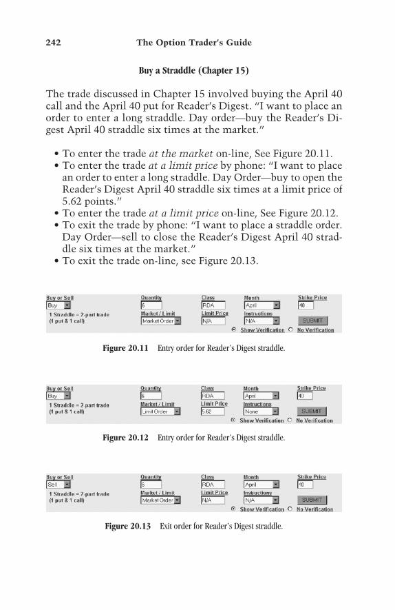
Buy a Straddle (Chapter 15)
The trade discussed in Chapter 15 involved buying the April 40call and the April 40 put for Reader’s Digest. “I want to place anorder to enter a long straddle. Day order—buy the Reader’s Di-gest April 40 straddle six times at the market.”
• To enter the trade at the market on-line, See Figure 20.11.• To enter the trade at a limit price by phone: “I want to place
an order to enter a long straddle. Day Order—buy to open theReader’s Digest April 40 straddle six times at a limit price of5.62 points.”
• To enter the trade at a limit price on-line, See Figure 20.12.• To exit the trade by phone: “I want to place a straddle order.
Day Order—sell to close the Reader’s Digest April 40 strad-dle six times at the market.”
• To exit the trade on-line, see Figure 20.13.
242 The Option Trader’s Guide
Figure 20.12 Entry order for Reader’s Digest straddle.
Figure 20.13 Exit order for Reader’s Digest straddle.
Figure 20.11 Entry order for Reader’s Digest straddle.
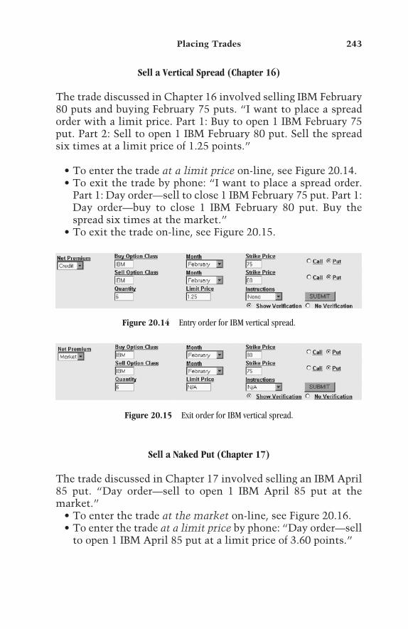
Sell a Vertical Spread (Chapter 16)
The trade discussed in Chapter 16 involved selling IBM February80 puts and buying February 75 puts. “I want to place a spreadorder with a limit price. Part 1: Buy to open 1 IBM February 75put. Part 2: Sell to open 1 IBM February 80 put. Sell the spreadsix times at a limit price of 1.25 points.”
• To enter the trade at a limit price on-line, see Figure 20.14.• To exit the trade by phone: “I want to place a spread order.
Part 1: Day order—sell to close 1 IBM February 75 put. Part 1:Day order—buy to close 1 IBM February 80 put. Buy thespread six times at the market.”
• To exit the trade on-line, see Figure 20.15.
Placing Trades 243
Figure 20.15 Exit order for IBM vertical spread.
Figure 20.14 Entry order for IBM vertical spread.
Sell a Naked Put (Chapter 17)
The trade discussed in Chapter 17 involved selling an IBM April85 put. “Day order—sell to open 1 IBM April 85 put at themarket.”
• To enter the trade at the market on-line, see Figure 20.16.• To enter the trade at a limit price by phone: “Day order—sell
to open 1 IBM April 85 put at a limit price of 3.60 points.”

• To enter the trade at a limit price on-line, See Figure 20.17.• To exit the trade by phone: “Day order—buy to close 1 IBM
April 85 put at the market.”• To exit the trade on-line, see Figure 20.18.
244 The Option Trader’s Guide
Figure 20.16 Entry order for IBM naked put.
Figure 20.17 Entry order for IBM naked put.
Figure 20.18 Exit order for IBM naked put.
Write a Covered Call (Chapter 18)
The following orders assume that you are already long 100 sharesof Computer Associates stock.
The trade discussed in Chapter 18 involved selling one Com-puter Associates February 35 call option, based on the assump-tion that you are already long 100 shares of Computer Associatesstock. “Day order—sell to open 1 Computer Associates February25 call at the market.”
• To enter the trade at the market on-line, see Figure 20.19.• To enter the trade at a limit price by phone: “Day order—sell
to open 1 Computer Associates February 25 call at a limitprice of 2.50 points.”
• To enter the trade at a limit price on-line, see Figure 20.20.
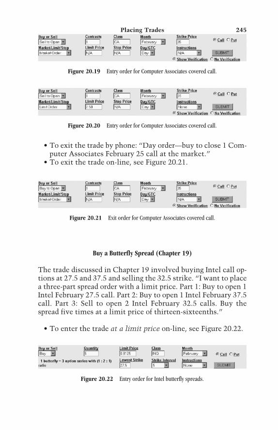
• To exit the trade by phone: “Day order—buy to close 1 Com-puter Associates February 25 call at the market.”
• To exit the trade on-line, see Figure 20.21.
Placing Trades 245
Figure 20.19 Entry order for Computer Associates covered call.
Figure 20.20 Entry order for Computer Associates covered call.
Figure 20.21 Exit order for Computer Associates covered call.
Figure 20.22 Entry order for Intel butterfly spreads.
Buy a Butterfly Spread (Chapter 19)
The trade discussed in Chapter 19 involved buying Intel call op-tions at 27.5 and 37.5 and selling the 32.5 strike. “I want to placea three-part spread order with a limit price. Part 1: Buy to open 1Intel February 27.5 call. Part 2: Buy to open 1 Intel February 37.5call. Part 3: Sell to open 2 Intel February 32.5 calls. Buy thespread five times at a limit price of thirteen-sixteenths.”
• To enter the trade at a limit price on-line, see Figure 20.22.

• To exit the trade by phone: “I want to place a three-partspread order. Part 1: Buy to close 2 Intel February 32.5 calls.Part 2: Sell to close one Intel February 27.5 call. Part 3: Sell toclose one Intel February 37.5 call. Sell the spread 5 times atthe market.”
• To exit the trade on-line, see Figure 20.23.
246 The Option Trader’s Guide
Figure 20.23 Exit order for Intel butterfly.
Summary
The examples presented in this chapter should not be taken asgospel. As noted earlier, different brokers use different protocolsfor option order placement. Before placing any option orders,double-check with your broker about format and wording thatshould be used for an order for any given trading strategy.

Epilogue
SOME RANDOM THOUGHTSFOR OPTION TRADERS
247
By now you should have some idea about what it takes to suc-ceed in option trading. You should know that there are certainbasic concepts that you must understand and apply properly ifyou hope to succeed in the long run. For example, until you un-derstand and appreciate the impact of time decay and volatilityon any option position you might consider, any success youenjoy in the short run is unlikely to last.
You should recognize that option trading can be significantlyand fundamentally different from simply buying and sellingstocks or futures contracts. A long stock position makes a pointeach time the stock rises a point and loses a point each time thestock falls a point. A given option position—depending on itsmakeup—might make a lot of money if the stock rises or falls,whereas another position will only make money if the stockdoes not rise or fall beyond a certain amount. Understandinghow to craft a position to achieve a particular objective is whatseparates the professional option trader from the masses hopingto buy a cheap option and hit a home run.
No one succeeds in trading because they got lucky on a tradeor two. Those who succeed consistently in the long run are thosewho make the effort and take the time to learn the skills re-quired to achieve lasting success. They apply these lessons in thereal world, trade after trade.
TEAMFLY
Team-Fly®

Real-world trading is a far different experience from papertrading or system development. Paper trading can be fun. Systemdevelopment can be intellectually stimulating. Trading in thereal world with real money on the line can be downright fright-ening. There is a feeling you get in the pit of your stomach whenthings go very wrong that cannot be described. When theprospect of losing money—especially big money—raises its uglyhead, emotion can take over and cause even the most rationaltrading veteran to throw the trading plan out the window andsimply react in an effort to stop the pain. You should recognizeby now the need to plan in advance for each trade’s worst casescenario before getting into the trade.
One of the best things you can do right now is to narrowdown the list of available option-trading strategies and deter-mine which ones you will be most comfortable using. Too manytraders dabble, trying a butterfly spread this week, a backspreadthe next, and so forth. This is no way to succeed.
You should also familiarize yourself with which strategiesare best used in a given situation. Want to pick a bottom, butyou’re afraid of an outright collapse by the underlying? If volatil-ity is low, consider a backspread. If volatility is high, considerselling a vertical spread, writing an option with a strike pricebelow the recent low. Is a stock putting you to sleep, wanderingin a narrow range between support and resistance? If volatility islow, consider a calendar spread. Think that it’s due for a break-out? Consider buying a straddle. Itching to buy a particular stockbut just can’t pull the trigger? If volatility is high, consider sell-ing a naked put. If volatility is low, consider buying a longer-term call option. Want to buy a call on a stock that you justknow is going to rally, but option volatility is going through theroof? Consider buying a shorter-term, deep-in-the-money call op-tion to minimize the amount of time premium you pay. Thepossibilities are endless.
You must also remember that getting into a trade is only onepart of the equation. In fact, in many instances selecting and en-tering a trade is the easy part. Sometimes big trends play out andtraders who cash out quickly miss out on big potential profits.At other times big profits on option trades exist for only a very
248 The Option Trader’s Guide

short time and then vanish forever. For this reason it is ab-solutely critical to your long-term success that you determinewhen you enter each trade what criteria you will use to exit thetrade. Without this type of planning, most traders are doomed toveering with each twist in the road.
Consistently applying the principles and concepts detailed inthis book offers you the greatest opportunity for consistent, long-term success. I wish you good fortune in achieving that goal.
Some Random Thoughts for Option Traders 249


Appendix A
PROVEST OPTION TRADINGMETHOD CRITERIA
251
The PROVEST Option Trading Method: A Frameworkfor Trade Selection
There are several key factors to consider in determining the bestoption-trading strategy to use at any given moment for a given un-derlying security. Selecting from the available strategies involvesknowing what to look for in terms of probability, volatility, timeto expiration, the skew of implied volatilities, and market move-ment. The PROVEST Option Trading Method was developed toidentify specific criteria in each of these key areas. The primaryfactors and key considerations are detailed in Table A.1.
By defining appropriate PROVEST factors for each of thetrading strategies, we create a structured approach to optionstrading. In turn, we can zero in on trades that generate the high-est probability of making money, rather than relying on gut feeland luck in the marketplace (see Table A.2).
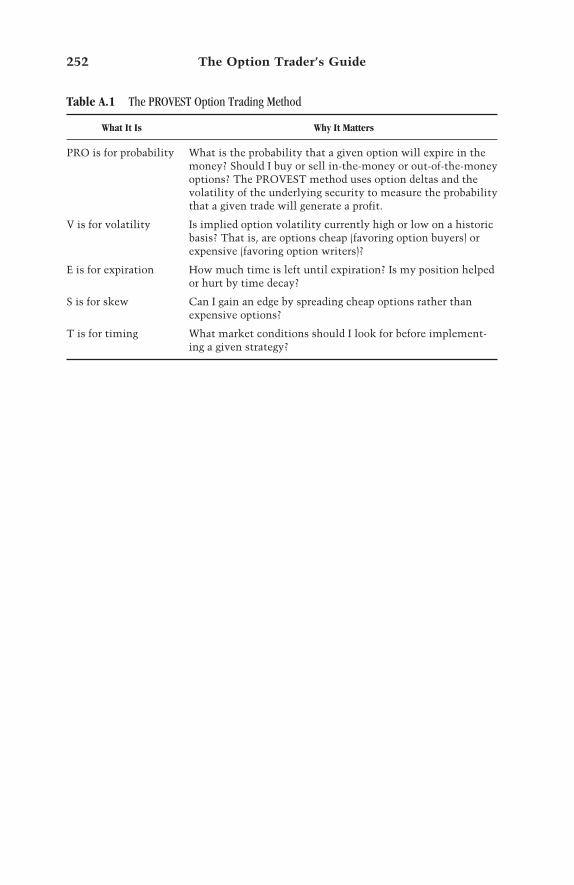
252 The Option Trader’s Guide
Table A.1 The PROVEST Option Trading Method
What It Is Why It Matters
PRO is for probability What is the probability that a given option will expire in themoney? Should I buy or sell in-the-money or out-of-the-moneyoptions? The PROVEST method uses option deltas and thevolatility of the underlying security to measure the probabilitythat a given trade will generate a profit.
V is for volatility Is implied option volatility currently high or low on a historicbasis? That is, are options cheap (favoring option buyers) orexpensive (favoring option writers)?
E is for expiration How much time is left until expiration? Is my position helpedor hurt by time decay?
S is for skew Can I gain an edge by spreading cheap options rather thanexpensive options?
T is for timing What market conditions should I look for before implement-ing a given strategy?

253
Tabl
e A.
2PR
OVE
ST O
ptio
n Tr
adin
g M
etho
d Su
mm
ary
Tabl
e
Stra
tegy
Del
taVo
latil
ityEx
pira
tion
Skew
Tim
ing
Bu
y n
aked
opti
ons
> 50
; Bu
yin
g in
-th
e-m
oney
opt
ion
s is
pref
erab
le. T
his
redu
ces
amou
nt
ofti
me
prem
ium
pai
das
a p
erce
nt
of o
ptio
npr
ice
and
incr
ease
spr
obab
ilit
y of
pro
fit.
Th
e lo
wer
th
e be
tter
.T
he
hig
her
th
evo
lati
lity
, th
e fu
rth
erin
th
e m
oney
an
d th
esh
orte
r te
rm t
he
opti
on y
ou b
uy
shou
ld b
e.
Dep
ends
on
tra
din
gti
me
fram
e; m
ust
be
care
ful
duri
ng
2w
eek
s be
fore
exp
ira-
tion
, as
tim
e de
cay
acce
lera
tes.
Not
rel
evan
t.O
nly
use
wh
en v
ery
bull
ish
or
very
bea
r-is
h.
Bu
y a
stra
ddle
Att
empt
to
mak
etr
ade
delt
a n
eutr
al;
you
wan
t an
equ
alch
ance
to
mak
em
oney
if
un
derl
yin
gri
ses
or f
alls
.
Th
e lo
wer
th
e be
tter
.R
edu
ces
amou
nt
you
pay,
in
crea
ses
you
rpr
obab
ilit
y of
pro
fit,
and
a ri
se i
n v
olat
il-
ity
can
hel
p.
74 d
ays
or m
ore.
Not
mea
nin
gfu
l.L
ook
for
ext
ende
dco
nso
lida
tion
(i.e
.,u
nde
rlyi
ng
is d
ue
for
a tr
end.
).
Bu
y a
back
spre
adA
ttem
pt t
o m
ake
trad
e de
lta
neu
tral
at
tim
e of
en
try;
gen
er-
ally
pre
fer
to w
rite
slig
htl
y in
-th
e-m
oney
opt
ion
s.
Low
er i
s be
tter
. Ari
se i
n v
olat
ilit
y ca
nh
elp
a lo
t; a
dec
lin
ein
vol
atil
ity
can
hu
rta
lot.
Bes
t to
bu
y lo
nge
r-te
rm o
ptio
ns
to l
imit
tim
e de
cay
wh
ile
wai
tin
g fo
r th
e u
n-
derl
yin
g to
mov
e.
Hig
her
vol
atil
ity
for
opti
on s
old
is a
plu
s.U
se w
hen
loo
kin
g fo
ra
mov
e in
a p
arti
cu-
lar
dire
ctio
n b
ut
not
com
fort
able
bu
yin
gn
aked
opt
ion
s.
Bu
y a
cale
nda
rsp
read
Del
ta o
f 35
to
65, o
rn
o m
ore
than
on
est
rik
e ou
t of
th
em
oney
.
Th
e lo
wer
th
e be
tter
.A
ris
e in
vol
atil
ity
can
hel
p tr
emen
-do
usl
y, a
dec
lin
e in
vola
tili
ty c
an b
edi
sast
rou
s.
≤45
days
.E
nte
r tr
ade
only
if
15%
hig
her
vol
atil
ity
for
opti
on s
old.
Loo
k f
or m
ean
ingf
ul
supp
ort
and
resi
st-
ance
lev
els
bou
ndi
ng
a tr
adin
g ra
nge
.
(con
tinue
s)

254
Tabl
e A.
2PR
OVE
ST O
ptio
n Tr
adin
g M
etho
d Su
mm
ary
Tabl
e (c
ontin
ued
)
Stra
tegy
Del
taVo
latil
ityEx
pira
tion
Skew
Tim
ing
Sell
ave
rtic
alsp
read
Cal
ls:≤
40 P
uts
: ≥–4
0 (i
.e.,
sell
ou
t-of
-th
e-m
oney
opt
ion
s).
Th
e h
igh
er t
he
bet-
ter.
Th
e h
igh
er t
he
vola
tili
ty, t
he
grea
ter
the
prof
it p
oten
tial
.
≤60
day
sId
eall
y a
hig
her
vola
tili
ty f
or o
ptio
nso
ld.
Loo
k f
or s
upp
ort
(or
resi
stan
ce) b
etw
een
un
derl
yin
g pr
ice
and
stri
ke
pric
e of
opt
ion
sold
.
Sell
nak
edpu
tsD
elta
> –
50 (i
.e. s
ell
out-
of-t
he-
mon
eyop
tion
s to
tak
e ad
-va
nta
ge o
f ti
me
deca
y).
Use
on
ly w
hen
vola
tili
ty i
sex
trem
ely
hig
h.
≤60
day
s.N
ot m
ean
ingf
ul.
Bes
t u
sed
wh
en a
stoc
k y
ou w
ant
tobu
y is
ove
rsol
d an
dvo
lati
lity
has
ex-
plod
ed.
Wri
te a
cove
red
call
≤40
for
opt
ion
s so
ld(i
.e.,
sell
ou
t-of
-th
e-m
oney
opt
ion
s to
tak
e ad
van
tage
of
tim
e de
cay)
.
On
ly w
rite
cov
ered
call
wh
en v
olat
ilit
yis
ext
rem
ely
hig
h t
om
axim
ize
the
amou
nt
of p
rem
ium
you
col
lect
.
≤60
day
s.N
ot m
ean
ingf
ul.
Bes
t u
sed
wh
envo
lati
lity
is
hig
h a
nd
un
derl
yin
g se
curi
tyis
ove
rbou
ght.
Bu
tter
fly
spre
adSe
ll s
ligh
tly
out-
of-
mon
ey o
ptio
n a
sm
iddl
e st
rik
e of
spre
ad.
Th
e h
igh
er, t
he
bett
er; t
rade
mak
esm
oney
fro
m t
ime
deca
y or
a d
ecli
ne
invo
lati
lity
, or
both
.
≤60
day
s, ≤
30 i
sev
en b
ette
r.Id
eal
if m
iddl
e op
tion
(i.e
., th
e on
e yo
uw
rite
) is
trad
ing
at a
hig
her
vol
atil
ity
than
the
opti
ons
you
bu
y.
Loo
k f
or m
ean
ingf
ul
supp
ort
and
resi
st-
ance
.

Appendix B
OPTION EXCHANGES, OPTIONBROKERS, OPTION SYMBOLS,
AND OPTION VOLUME
255
Exchanges
Options are traded at each of the exchanges listed in Tables B.1and B.2.
Table B.1 Stock and Stock Index Option Exchanges
Exchange Web Site
Chicago Board Options Exchange (CBOE) www.cboe.comAmerican Stock Exchange www.options.nasdaq-amex.comPhiladelphia Stock Exchange www.phlx.comPacific Stock Exchange www.pacificex.com
Table B.2 Exchanges Trading Futures Options
Exchange Web Site
Chicago Board of Trade www.cbot.comChicago Mercantile Exchange www.cme.comCOMEX (Metals) www.nymex.comNew York Board of Trade www.nybot.comNew York Mercantile Exchange (Energies) www.nymex.com

256 The Option Trader’s Guide
Tabl
e B.
3Br
oker
s D
ealin
g in
Sto
ck a
nd S
tock
Inde
x O
ptio
ns
Firm
Web
Site
Phon
eAc
coun
t Min
imum
Com
mis
sion
s
A-1
Fin
anci
alw
ww
.a1f
inan
cial
.com
877-
a1-f
inan
cial
$100
0$2
3 +
$2.5
0 pe
r co
ntr
act
Acc
utr
ade
ww
w.a
ccu
trad
e.co
m80
0-49
4-89
49$5
000
$35;
$1.
5 to
$8
per
con
trac
t
Am
erit
rade
ww
w.a
mer
itra
de80
0-66
9-39
00$2
000
$25+
$1.7
5 pe
r co
ntr
act
($29
min
imu
m)
Ben
jam
in &
Jer
old
ww
w.s
tock
opti
ons.
com
800-
446-
5112
$500
0$1
.50
to $
5.90
per
con
trac
t ($
36 m
inim
um
)
Bro
wn
& C
o.w
ww
.bro
wn
co.c
om80
0-35
7-44
10$1
5,00
0$1
5 +
$1.5
0 pe
r co
ntr
act
($25
min
imu
m)
Com
puT
EL
Sec
uri
ties
ww
w.c
ompu
tel.
com
800-
432-
0327
$500
0$2
4 +
$1 p
er c
ontr
act
Dre
yfu
s B
rok
erag
e Se
rvic
esw
ww
.edr
eyfu
s.co
m80
0-42
1-83
95$2
000
$15
+ $1
.75
per
con
trac
t
Mr.
Sto
ckw
ww
.mrs
tock
.com
800-
470-
1896
$200
0$1
4.95
+ $
1.50
per
con
trac
t
Pre
ferr
ed T
rade
ww
w.p
refe
rred
trad
e.co
m80
0-94
9-35
04$1
000
$19.
95, o
r $2
.50
to $
3.00
per
con
trac
t
Qu
ick
& R
eill
yw
ww
.qu
ick
-rei
lly.
com
800-
221-
7220
Non
e$3
7.50
plu
s $1
.75
per
con
trac
t
Sch
wab
On
Lin
ew
ww
.esc
hw
ab.c
om80
0-43
5-40
00$2
500
$35
+ 1.
75 p
er c
ontr
act
Wal
l St
reet
Acc
ess
ww
w.w
sacc
ess.
com
800-
925-
5781
$10,
000
$25
plu
s $1
.50
to $
2.50
per
con
trac
t
Wal
l St
reet
Ele
ctro
nic
aw
ww
.wal
lstr
eete
.com
888-
925-
5783
$250
0 to
$2
5 pl
us
$2.5
0 pe
r co
ntr
act
$10,
000

Option Exchanges, Option Brokers, Option Symbols 257
Brokerage Firms
Most brokerage firms offer you the capability of trading options,but not all firms offer the same level of commitment to optiontrading. Tables B.3 and B.4 present a short list of brokerage firmsthat offer option trading or even emphasize it.
Table B.4 Brokers Dealing in Futures Options
Firm Web Site Phone
Jack Carl www.jackcarl.com 800-621-3424Lind-Waldock www.lind-waldock.com 800-445-2000NetFutures www.netfutures.com 800-872-6673Peregrine Financial Group www.pfg.com 800-333-5673Professional Market Brokerage www.pmbinc.com 800-672-2462Robbins Trading www.robbinstrading.com 800-453-4444Zap Futures www.zapfutures.com 800-441-1616
Resources
Other helpful sites can be found in Table B.5.
Table B.5
Firm Web Site What It Offers
Chicago Board Options www.cboe.com Exchange specific Exchange (CBOE) quotes, education,
and strategiesOptions Clearing Corporation www.optionsclearing.com Information from the
company that clears executions for all exchanges
New Options Onn.theocc.com/series/ Lists new options pgms/todays_add.pl from the Options
Clearing CorporationOptions Industry Council www.optionscentral.com AMEX, CBOE, PCX,
and PHLX joined to create this educa-tional site for option traders
Author’s Company Web sites www.essextrading.com Various trading-www.essexcta.com related information
(continues)
TEAMFLY
Team-Fly®

Table B.5 (continued)
Firm Web Site What It Offers
Books on Trading www.traderslibrary.com Trading books and tapes
Web Investor Options Directory www.thewebinvestor.com Links to advisories, brokers, newsletters, and software
Charting and Education www.echarts.com Charting and educa-tional materials
Charting and News www.barcharts.com Charting and company information
Technical Analysis of Stocks www.traders.com Articles related to and Commodities trading
Active Trader magazine www.activetradermag.com Articles related to trading
Futures magazine www.futuresmag.com Articles related to trading
Stock and Stock Index Option Symbols
Table B.6 lists all the available options for America Online(symbol: AOL) as of December 28, 2000. Due to stock price splitsand large price movements there are three different option rootsymbols: AOE, AOO, AOL. To place an option order on-line youmust use the appropriate root symbol. The best source of this in-formation is the following link via the CBOE: http://quote.cboe.com/quotetable.htm.
1. Go to this link and enter the underlying stock symbol.2. Click “List all options and LEAPS.”3. Click “Submit.”
To download this information, follow Steps 1 and 2 above,then click “Download Text File.” Enter the underlying stocksymbol again and click “Download.”
Stock Option Volume Statistics
Table B.7 gives you some idea of the level of option trading vol-ume among the most actively traded stocks.
258 The Option Trader’s Guide

259
Tabl
e B.
6Am
eric
a O
nlin
e O
ptio
ns A
vaila
ble
on D
ecem
ber
28, 2
000
Opt
ion
Expi
ratio
nEx
pira
tion
Stri
keCa
ll/O
ptio
nEx
pira
tion
Expi
ratio
nSt
rike
Call/
Sym
bol
Mon
thYe
arPr
ice
Put
Sym
bol
Mon
thYe
arPr
ice
Put
AO
L A
A1
15
CA
OL
MA
11
5P
AO
L A
Y1
15.
625
CA
OL
MY
11
5.62
5P
AO
L A
Z1
16.
25C
AO
L M
Z1
16.
25P
AO
L A
E1
16.
875
CA
OL
ME
11
6.87
5P
AO
L A
U1
17.
5C
AO
L M
U1
17.
5P
AO
L A
F1
18.
125
CA
OL
MF
11
8.12
5P
AO
L A
G1
18.
75C
AO
L M
G1
18.
75P
AO
L A
H1
19.
375
CA
OL
MH
11
9.37
5P
AO
L A
B1
110
CA
OL
MB
11
10P
AO
L A
I1
110
.625
CA
OL
MI
11
10.6
25P
AO
L A
J1
111
.25
CA
OL
MJ
11
11.2
5P
AO
L A
K1
111
.875
CA
OL
MK
11
11.8
75P
AO
L A
V1
112
.5C
AO
L M
V1
112
.5P
AO
L A
L1
113
.125
CA
OL
ML
11
13.1
25P
AO
L A
M1
113
.75
CA
OL
MM
11
13.7
5P
AO
L A
C1
115
CA
OL
MC
11
15P
AO
L A
O1
115
.625
CA
OL
MO
11
15.6
25P
AO
L A
P1
116
.25
CA
OL
MP
11
16.2
5P
AO
L A
Q1
116
.875
CA
OL
MQ
11
16.8
75P
AO
L A
W1
117
.5C
AO
L M
W1
117
.5P
AO
L A
R1
118
.125
CA
OL
MR
11
18.1
25P
AO
L A
S1
118
.75
CA
OL
MS
11
18.7
5P
AO
L A
T1
119
.375
CA
OL
MT
11
19.3
75P
AO
L A
D1
120
CA
OL
MD
11
20P
AO
L B
D2
120
CA
OL
ND
21
20P
AO
L D
D4
120
CA
OL
PD
41
20P
(con
tin
ues
)

260
Tabl
e B.
6Am
eric
a O
nlin
e O
ptio
ns A
vaila
ble
on D
ecem
ber
28, 2
000
(Con
tinu
ed)
Opt
ion
Expi
ratio
nEx
pira
tion
Stri
keCa
ll/O
ptio
nEx
pira
tion
Expi
ratio
nSt
rike
Call/
Sym
bol
Mon
thYe
arPr
ice
Put
Sym
bol
Mon
thYe
arPr
ice
Put
AO
L G
D7
120
CA
OL
SD
71
20P
AO
L A
N1
121
.25
CA
OL
MN
11
21.2
5P
AO
L A
X1
122
.5C
AO
L M
X1
122
.5P
AO
L B
X2
122
.5C
AO
L N
X2
122
.5P
AO
L D
X4
122
.5C
AO
L P
X4
122
.5P
AO
L G
X7
122
.5C
AO
L S
X7
122
.5P
AO
E A
K1
123
.75
CA
OE
MK
11
23.7
5P
AO
E A
E1
125
CA
OE
ME
11
25P
AO
E B
E2
125
CA
OE
NE
21
25P
AO
E D
E4
125
CA
OE
PE
41
25P
AO
E G
E7
125
CA
OE
SE
71
25P
AO
E A
L1
126
.25
CA
OE
ML
11
26.2
5P
AO
E A
Y1
127
.5C
AO
E M
Y1
127
.5P
AO
E B
Y2
127
.5C
AO
E N
Y2
127
.5P
AO
E D
Y4
127
.5C
AO
E P
Y4
127
.5P
AO
E G
Y7
127
.5C
AO
E S
Y7
127
.5P
AO
E A
M1
128
.75
CA
OE
MM
11
28.7
5P
AO
E A
F1
130
CA
OE
MF
11
30P
AO
E B
F2
130
CA
OE
NF
21
30P
AO
E D
F4
130
CA
OE
PF
41
30P
AO
E G
F7
130
CA
OE
SF
71
30P
AO
E A
N1
131
.25
CA
OE
MN
11
31.2
5P
AO
E A
Z1
132
.5C
AO
E M
Z1
132
.5P
AO
E B
Z2
132
.5C
AO
E N
Z2
132
.5P
AO
E D
Z4
132
.5C
AO
E P
Z4
132
.5P
AO
E G
Z7
132
.5C
AO
E S
Z7
132
.5P
AO
E A
O1
133
.75
CA
OE
MO
11
33.7
5P

261
AO
E A
G1
135
CA
OE
MG
11
35P
AO
E B
G2
135
CA
OE
NG
21
35P
AO
E D
G4
135
CA
OE
PG
41
35P
AO
E G
G7
135
CA
OE
SG
71
35P
AO
E A
U1
137
.5C
AO
E M
U1
137
.5P
AO
E B
U2
137
.5C
AO
E N
U2
137
.5P
AO
E D
U4
137
.5C
AO
E P
U4
137
.5P
AO
E G
U7
137
.5C
AO
E S
U7
137
.5P
AO
E A
H1
140
CA
OE
MH
11
40P
AO
E B
H2
140
CA
OE
NH
21
40P
AO
E D
H4
140
CA
OE
PH
41
40P
AO
E G
H7
140
CA
OE
SH
71
40P
AO
E A
R1
141
.25
CA
OE
MR
11
41.2
5P
AO
E A
V1
142
.5C
AO
E M
V1
142
.5P
AO
E B
V2
142
.5C
AO
E N
V2
142
.5P
AO
E D
V4
142
.5C
AO
E P
V4
142
.5P
AO
E G
V7
142
.5C
AO
E S
V7
142
.5P
AO
E A
S1
143
.75
CA
OE
MS
11
43.7
5P
AO
E A
I1
145
CA
OE
MI
11
45P
AO
E B
I2
145
CA
OE
NI
21
45P
AO
E D
I4
145
CA
OE
PI
41
45P
AO
E G
I7
145
CA
OE
SI
71
45P
AO
E A
T1
146
.25
CA
OE
MT
11
46.2
5P
AO
E A
W1
147
.5C
AO
E M
W1
147
.5P
AO
E B
W2
147
.5C
AO
E N
W2
147
.5P
AO
E D
W4
147
.5C
AO
E P
W4
147
.5P
AO
E G
W7
147
.5C
AO
E S
W7
147
.5P
AO
E A
X1
148
.75
CA
OE
MX
11
48.7
5P
AO
O A
J1
150
CA
OO
MJ
11
50P
AO
O B
J2
150
CA
OO
NJ
21
50P
AO
O D
J4
150
CA
OO
PJ
41
50P
(con
tin
ues
)

262
Tabl
e B.
6Am
eric
a O
nlin
e O
ptio
ns A
vaila
ble
on D
ecem
ber
28, 2
000
(Con
tinu
ed)
Opt
ion
Expi
ratio
nEx
pira
tion
Stri
keCa
ll/O
ptio
nEx
pira
tion
Expi
ratio
nSt
rike
Call/
Sym
bol
Mon
thYe
arPr
ice
Put
Sym
bol
Mon
thYe
arPr
ice
Put
AO
O G
J7
150
CA
OO
SJ
71
50P
AO
O A
E1
152
.5C
AO
O M
E1
152
.5P
AO
O A
K1
155
CA
OO
MK
11
55P
AO
O B
K2
155
CA
OO
NK
21
55P
AO
O D
K4
155
CA
OO
PK
41
55P
AO
O G
K7
155
CA
OO
SK
71
55P
AO
O A
F1
157
.5C
AO
O M
F1
157
.5P
AO
O A
L1
160
CA
OO
ML
11
60P
AO
O B
L2
160
CA
OO
NL
21
60P
AO
O D
L4
160
CA
OO
PL
41
60P
AO
O G
L7
160
CA
OO
SL
71
60P
AO
O A
G1
162
.5C
AO
O M
G1
162
.5P
AO
O A
M1
165
CA
OO
MM
11
65P
AO
O B
M2
165
CA
OO
NM
21
65P
AO
O D
M4
165
CA
OO
PM
41
65P
AO
O G
M7
165
CA
OO
SM
71
65P
AO
O A
N1
170
CA
OO
MN
11
70P
AO
O B
N2
170
CA
OO
NN
21
70P
AO
O D
N4
170
CA
OO
PN
41
70P
AO
O G
N7
170
CA
OO
SN
71
70P
AO
O A
O1
175
CA
OO
MO
11
75P
AO
O B
O2
175
CA
OO
NO
21
75P
AO
O D
O4
175
CA
OO
PO
41
75P
AO
O G
O7
175
CA
OO
SO
71
75P
AO
O A
W1
177
.5C
AO
O M
W1
177
.5P
AO
O A
P1
180
CA
OO
MP
11
80P
AO
O B
P2
180
CA
OO
NP
21
80P

263
AO
O D
P4
180
CA
OO
PP
41
80P
AO
O G
P7
180
CA
OO
SP
71
80P
AO
O A
X1
182
.5C
AO
O M
X1
182
.5P
AO
O A
Q1
185
CA
OO
MQ
11
85P
AO
O B
Q2
185
CA
OO
NQ
21
85P
AO
O D
Q4
185
CA
OO
PQ
41
85P
AO
O G
Q7
185
CA
OO
SQ
71
85P
AO
O A
Y1
187
.5C
AO
O M
Y1
187
.5P
AO
O A
R1
190
CA
OO
MR
11
90P
AO
O B
R2
190
CA
OO
NR
21
90P
AO
O D
R4
190
CA
OO
PR
41
90P
AO
O G
R7
190
CA
OO
SR
71
90P
AO
O A
Z1
192
.5C
AO
O M
Z1
192
.5P
AO
O A
S1
195
CA
OO
MS
11
95P
AO
O A
T1
110
0C
AO
O M
T1
110
0P
AO
O A
A1
110
5C
AO
O M
A1
110
5P
AO
O A
B1
111
0C
AO
O M
B1
111
0P
AO
O A
C1
111
5C
AO
O M
C1
111
5P
AO
O A
D1
112
0C
AO
O M
D1
112
0P
AO
W A
E1
112
5C
AO
W M
E1
112
5P
AO
W A
F1
113
0C
AO
W M
F1
113
0P
AO
W A
G1
113
5C
AO
W M
G1
113
5P
AO
W A
H1
114
0C
AO
W M
H1
114
0P
AO
W A
I1
114
5C
AO
W M
I1
114
5P

264
Tabl
e B.
7Av
erag
e D
aily
Sto
ck O
ptio
n Vo
lum
e on
CBO
E in
Apr
il 20
01
Aver
age
Aver
age
Aver
age
Opt
ion
Stoc
kM
onth
lyD
aily
Dai
lyD
aily
Sym
bol
Sym
bol
Stoc
k Na
me
Volu
me
Volu
me
Call
Volu
me
Put V
olum
e
MSQ
MSF
TM
icro
soft
Cor
pora
tion
1,15
7,35
957
,868
35,4
5322
,415
CY
QC
SCO
Cis
co S
yste
ms,
In
c.99
0,05
449
,503
30,0
1219
,490
EM
CE
MC
EM
C C
orpo
rati
on50
1,17
325
,059
14,2
1510
,844
IBM
IBM
Inte
rnat
ion
al B
usi
nes
s M
ach
ines
Cor
pora
tion
485,
032
24,2
5212
,762
11,4
90A
OL
AO
LA
OL
Tim
e W
arn
er, I
nc.
445,
875
22,2
9415
,810
6484
OR
QO
RC
LO
racl
e C
orpo
rati
on40
7,14
920
,357
15,6
3647
21G
EG
EG
ener
al E
lect
ric
Com
pan
y40
4,37
720
,219
12,2
3279
87IN
QIN
TC
Inte
l C
orpo
rati
on39
4,55
319
,728
12,0
0377
25L
UL
UL
uce
nt
Tec
hn
olog
ies,
In
c.32
8,99
616
,450
12,3
4241
07D
LQ
DE
LL
Del
l C
ompu
ter
Cor
p.32
8,26
416
,413
10,3
7060
43JU
PJN
PR
Jun
iper
Net
wor
ks,
In
c.30
4,83
515
,242
6028
9214
CC
Cit
igro
up,
In
c.29
9,26
514
,963
9176
5787
NO
KN
OK
Nok
ia C
orpo
rati
on A
DR
279,
137
13,9
5710
,489
3468
QA
CO
MQ
UA
LC
OM
M, I
nc.
265,
316
13,2
6681
1851
48E
UQ
CIE
NC
ien
a C
orpo
rati
on26
0,38
013
,019
6260
6759
UQ
DJD
SUJD
S U
nip
has
e C
orp.
249,
842
12,4
9285
7339
19G
LW
GL
WC
orn
ing
Inco
rpor
ated
222,
847
11,1
4270
0841
34N
TN
TN
orte
l N
etw
ork
s C
orpo
rati
on22
0,40
411
,020
6702
4319
SUQ
SUN
WSu
n M
icro
syst
ems
Inc.
217,
373
10,8
6983
6925
00T
XN
TX
NT
exas
In
stru
men
ts I
nco
rpor
ated
217,
255
10,8
6375
803,
283
UB
FB
RC
DB
roca
de C
omm
un
icat
ion
s20
9,64
910
,482
8683
1800
SGQ
SEB
LSi
ebel
Sys
tem
s, I
nc.
202,
943
10,1
476,
070
4,07
7L
DQ
WC
OM
Wor
ldco
m, I
nc.
163,
137
8157
6157
2000
TT
AT
&T
Cor
pora
tion
156,
237
7812
4862
2950
VU
QV
RT
SV
ER
ITA
S So
ftw
are
Cor
pora
tion
153,
082
7654
3196
4458
YH
QY
HO
OY
ahoo
! In
c14
9,11
274
5649
1725
39M
OT
MO
TM
otor
ola,
In
c.14
0,52
970
2648
4521
82A
NQ
AM
AT
App
lied
Mat
eria
ls, I
nc.
138,
661
6,93
325
8543
48A
MD
AM
DA
dvan
ced
Mic
ro D
evic
es, I
nc.
136,
242
6,81
247
5020
62

INDEX
265
ADX DMI indicator, 105American style options, 108Ask price, 47, 110–111Assignment, 108, 109At-the-money option, 24Automatic exercise, 108Average implied volatility,
67–68
Backspread, 110buying, 151–164
backspreads versus nakedcalls and puts, 157–158,158 (figs.)
key factors, 151–157, 153(fig.), 154 (tab.), 155 (fig.),156 (fig.)
position management, 162,162 (tab.), 163 (fig.)
postition taken, 157purpose, 151trade result, 164volatility and backspreads,
159–162, 159 (fig.), 160(fig.), 161 (fig.)
Bear call spread, 192Bid-ask spread, 47
effect of, 111–113, 112 (tab.)
Bid prices, 47, 110–111Big hit, avoiding, 10, 11Black-Scholes model, 48, 49Break-even analysis, and proba-
bility of profit, 8Bull put spread, 192Butterfly spread, entering,
223–235key factors, 223–229, 226
(fig.), 227, (fig.), 227 (tab.),228 (fig.)
position management,233–234, 233 (tab.), 234(figs.)
position taken, 229–232, 232(fig.)
purpose, 223trade result, 235
Buy premium, 24, 73
Calculated volatility, 63Calendar spread, 44
buying, 165–177key factors, 165–173, 168
(tab.), 169 (fig.), 170 (figs.)position management,
173–174, 174 (fig.)position taken, 173
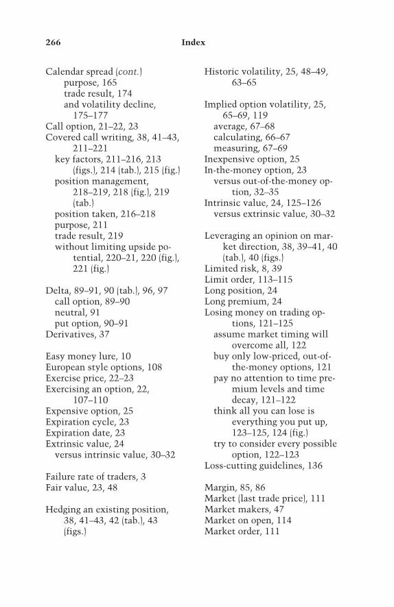
Calendar spread (cont.)purpose, 165trade result, 174and volatility decline,
175–177Call option, 21–22, 23Covered call writing, 38, 41–43,
211–221key factors, 211–216, 213
(figs.), 214 (tab.), 215 (fig.)position management,
218–219, 218 (fig.), 219(tab.)
position taken, 216–218purpose, 211trade result, 219without limiting upside po-
tential, 220–21, 220 (fig.),221 (fig.)
Delta, 89–91, 90 (tab.), 96, 97call option, 89–90neutral, 91put option, 90–91
Derivatives, 37
Easy money lure, 10European style options, 108Exercise price, 22–23Exercising an option, 22,
107–110Expensive option, 25Expiration cycle, 23Expiration date, 23Extrinsic value, 24
versus intrinsic value, 30–32
Failure rate of traders, 3Fair value, 23, 48
Hedging an existing position,38, 41–43, 42 (tab.), 43(figs.)
Historic volatility, 25, 48–49,63–65
Implied option volatility, 25,65–69, 119
average, 67–68calculating, 66–67measuring, 67–69
Inexpensive option, 25In-the-money option, 23
versus out-of-the-money op-tion, 32–35
Intrinsic value, 24, 125–126versus extrinsic value, 30–32
Leveraging an opinion on mar-ket direction, 38, 39–41, 40(tab.), 40 (figs.)
Limited risk, 8, 39Limit order, 113–115Long position, 24Long premium, 24Losing money on trading op-
tions, 121–125assume market timing will
overcome all, 122buy only low-priced, out-of-
the-money options, 121pay no attention to time pre-
mium levels and timedecay, 121–122
think all you can lose iseverything you put up,123–125, 124 (fig.)
try to consider every possibleoption, 122–123
Loss-cutting guidelines, 136
Margin, 85, 86Market (last trade price), 111Market makers, 47Market on open, 114Market order, 111
266 Index

Market timing, 99–106, 120,122
underlying expected to movebut direction isunknown, 103–105, 104(fig.)
underlying expected to movein particular direction butnot in specific timeframe, 102–103, 103 (fig.)
underlying expected to staywithin a range or notmove much, 105–106,106 (fig.)
underlying security move-ment within specificperiod, 100–102, 102 (fig.)
Maximum risk, 8Momentum investors, 202
Naked option, 25, 38, 81, 82, 85,86
buying, 139–150key factors, 139–146, 142
(fig.), 143 (fig.), 144 (tab.),145 (tab.)
position management,148–150, 149 (fig.), 149(tab.)
position taken, 146–148purpose, 139trade result, 150
versus backspreads, 157–158Naked put, selling, 201–209
key factors, 201–206, 203(fig.), 204 (fig.), 205 (tab.),205 (fig.)
one method for managingstock position if assigned,208
position management, 209position taken, 206–208trade result, 209, 209 (fig.)
Neutral situations, taking ad-vantage of, 38, 44–45, 44(tab.), 45 (figs.)
Objective approach, 4–6Option buyer, 22Option Clearing Corporation,
108, 219Option premium, 22Option price grid, 134, 135 (tab.)Option pricing, 47–53, 118
examples of theoretical op-tion pricing, 49–50, 50(tab.), 51 (tab.)
overvalued options versusundervalued options, 50,52, 52 (tab.)
theoretical value, 47–49Options
basics of, 21–35in-the-money versus out-of-
the-money options,32–35, 32 (fig.), 33 (figs.),34 (tabs.)
intrinsic value versus ex-trinsic value, 30–32, 31(tab.)
option definitions, 21–25options on specific security,
26–30, 26 (tab.)call options, 27–28, 27(figs.), 28 (fig.)put options, 28–30, 29(figs.), 30 (fig.)
three primary uses of, 37–38types of
American style, 108at-the-money, 24call, 21–22, 23European style, 108expensive, 25inexpensive, 25in-the-money, 23, 32–35
Index 267
TEAMFLY
Team-Fly®

Options, types of (cont.)naked, 25, 38, 81, 82, 85,
86, 139–150, 157–158out-of-the-money, 23–24,
32–35, 121overvalued, 25, 50, 52put, 22, 23undervalued, 25, 50, 52
Option tradingoverview of, 3–6
benefits of objective ap-proach, 4–6
successful, 125–128Option volatility graph, 134,
135 (fig.)Option writer, 22Order placement, 237Out-of-the-money option,
23–24, 121versus in-the-money option,
32–35Overvalued option, 25
versus undervalued option,50, 52
Placing trades, 237–246considerations in placing op-
tion orders, 238placing orders by phone or on
line, 238–246buy a backspread, 239buy a butterfly spread,
245–246buy a calendar spread, 241buy a straddle, 242buy naked calls or puts, 239sell a naked put, 243–244sell a vertical spread, 243write a covered call,
244–245Position, types of
long, 24short, 24
spread, 25Position-management consider-
ations, 136Premium, types of
buy, 24long, 24option, 22sell, 24short, 24time, 24, 55–56, 58, 81,
121–122Price, types of
ask, 47, 110–111bid, 47, 110–111exercise, 22–23strike, 21, 22–23, 77theoretical, 23, 47–49theoretical option, 48, 49–50
Probability, 81–97, 120analysis, 91–95, 92 (figs.), 93
(fig.), 94 (fig.), 95 (tab.)correct and incorrect ways to
use, 95–96delta, 89–91profit/loss comparisons,
86–89, 87 (figs.), 88 (fig.),88 (tabs.)
strategies for bullish scenario,82–86, 83 (figs.), 84 (fig.)
buying 100 shares at 94,83–84
buying 1 February 90 calloption at 9.88, 84
writing 10 February 75 putoptions at 1.375, 85
weighing pros and cons,81–82
Probability of profit, and break-even analysis, 8
Profit/loss comparisons, 86–89,87 (figs.), 88 (fig.), 88(tabs.)
Profit potential, 8–9
268 Index

Profit-taking guidelines, 136PROVEST Option Trading
Method, 131, 251–254Put option, 22, 23
Ratio spread, 12–16, 13 (fig.), 14(fig.)
Reasons to trade options, 37–46,117–118
Relative volatility, 69–72ranking, 72
Riskanalyzing, 11–18
Case 1: ratio spread, 12–16,13 (fig.), 14 (fig.)
Case 2: synthetic long fu-tures position, 16–18, 16(fig.), 17 (fig.)
limited, 8maximum, 8mitigating, 9and reward, 82, 97
Risk curves, 6–9, 7 (fig.), 9 (fig.)break-even analysis and prob-
ability of profit, 8effect of time decay, 7–8graph, 134, 136, 136 (tab.)maximum risk, 8profit potential, 8–9
Roll down, 217
Sell premium, 24, 73Short position, 24Short premium, 24Skew, 67
of implied volatilities, 73–74Spread, types of
bear call spread, 192bid-ask, 47, 111–113bull put spread, 192butterfly, 223–235calendar, 44, 165–177vertical, 191–200
Spread position, 25Statistical volatility, 63Straddle, 91, 94, 95, 103
buying, 179–190key factors, 179–186, 182
(fig.), 183 (fig.), 184 (fig.),185 (tab.)
position management,188–189, 188 (tab.), 189(fig.)
position taken, 186–188purpose, 179trade result, 189
Strangle, 179Strike price, 21, 22–23
volatility and, 77Successful option trading,
125–128buy options with intrinsic
value, 125–126concentrate on stocks with
active option volume,128
identify most useful tradingstrategies, 127–128
key trading guidelines, 125write options made up of time
premium, 126–127Synthetic long futures position,
16–18, 16 (fig.), 17 (fig.)
Theoretical option price, 48,49–50
Theoretical price, 23, 47–49Theoretical value, 47–49Time decay, 52, 55–62, 119,
121–122effect of, 7–8, 56–58, 57 (tab.),
57 (figs.)illustration of, 58–62, 59
(figs.), 60 (figs.), 61 (figs.),62 (tab.)
implications of, 58
Index 269

Time premium, 24, 31, 55–56,58, 81, 121–122
Trading options, reasons for,37–46, 117–118
three primary uses of options,37–38
hedging an existing position(and generating income),38, 41–43, 42 (tab.), 43(figs.)
leveraging an opinion onmarket direction, 38,39–41, 40 (tab.), 40 (figs.)
taking advantage of neutralsituations, 38, 44–45, 44(tab.), 45 (figs.)
Trading plan, 4–6, 128–129Trading realities, 107–116
bid and ask prices and impor-tance of option volume,110–111
effect of bid-ask spreads,111–113, 112 (tab.)
exercise and assignment,107–110
example of a trade, 110implications of exercise,
107–110when to expect an option to
be exercised, 109factors in dealing with bid-ask
spreads, 113, 113 (tab.)limit orders, 113–115
Trading strategymatrix, 132 (tab.), 133two key elements in select-
ing, 131–132
Underlying price action graph,134, 134 (fig.)
Underlying security, 22Undervalued option, 25
versus overvalued option, 50,52
Value, types ofextrinsic, 24intrinsic, 24, 125–126theoretical, 47–49
Value investors, 202Vertical spread, selling,
191–200key factors, 191–197, 194
(figs.), 195 (tab.), 196 (fig.)position management,
199–200, 200 (figs.)position taken, 197–199purpose, 191trade result, 200
Volatility, 63–80, 119–120, 132
and backspreads, 159–162and calendar spreads,
175–177considerations in selecting
option-trading strategies,72–74
current implied volatilityand relative volatilityrank, 72–73
skew of implied volatilities,73–74, 74 (fig.)
effect of changes in, 77–80, 78(tabs.), 79 (tabs.)
historical, 63–65, 64 (fig.), 65(fig.)
implications of, 74–77, 75(tabs.), 76 (figs.), 77 (tabs.)
implied, 65–69average, 67–68calculating, 66–67measuring, 67–69, 68 (tab.)
importance of, in option trad-ing, 63
270 Index

relative, 69–72, 70 (fig.), 71(fig.)
ranking, 72, 72 (fig.)skew, 67types of
average implied, 67–68calculated, 63historical, 25, 48–49, 63–65implied option, 25, 65–69,
119
relative, 69–72statistical, 63
Wasting asset, 3, 191Welles Wilder’s ADX Direc-
tional Movement Index(DMI), 101, 105
Worst-case scenario, 9, 11, 15,86
Writing a contract, 24
Index 271


