
The Path Integral for
Relativistic WorldlinesB. Koch
with E. Muñoz and I. Reyes based on:
Phys.Rev. D96 (2017) no.8, 085011 and arXiv:1706.05388.
1
Afunalhue, La parte y el todo, 2018

Content
PI of the RPP, Status
Local Symmetry: Velocity Rotations
Constructing the PI of the RPP
Conclusion
2

The Path Integral
A B
Propagator
hA|Bi ⇠Z
Dx e
�SA,B
(after Wick rotation)3
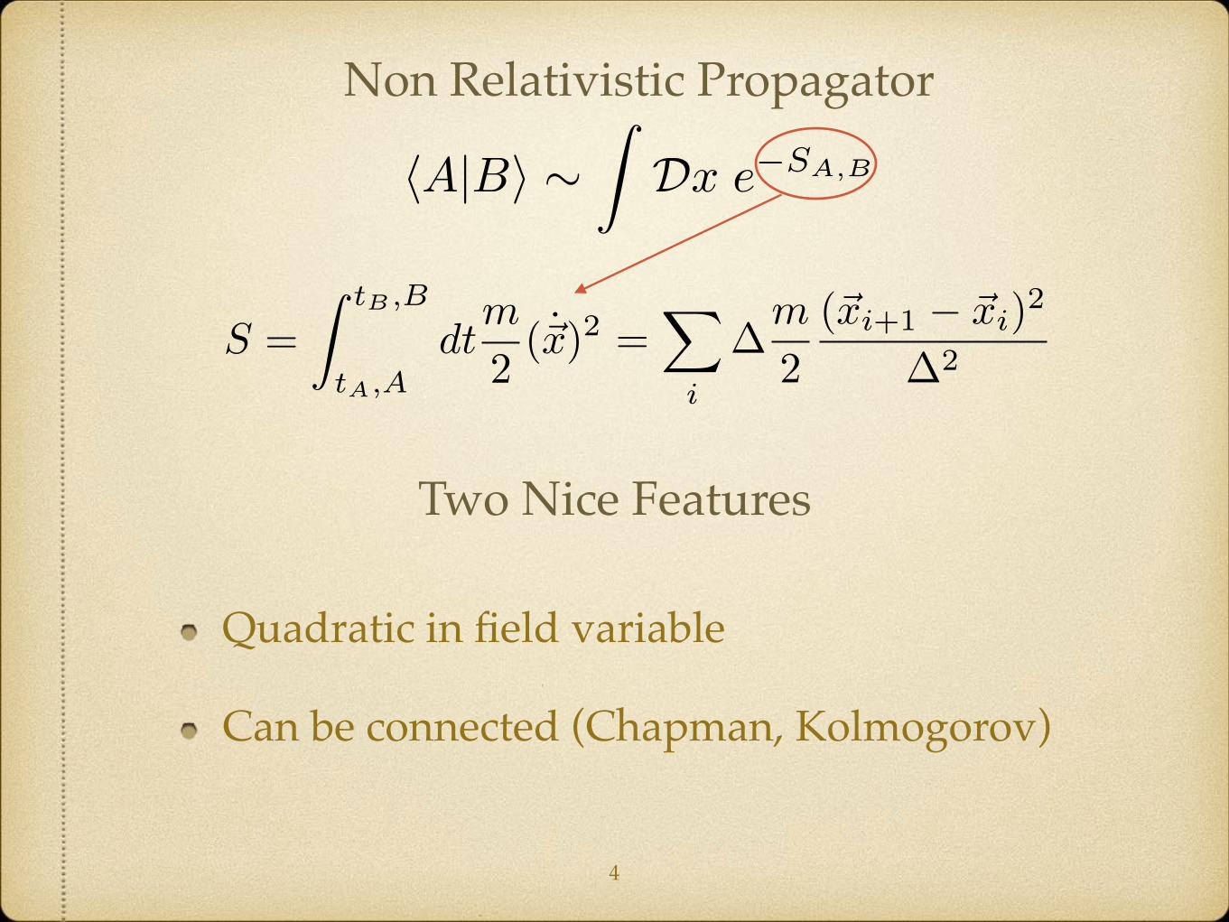
Non Relativistic Propagator
S =
Z tB ,B
tA,Adt
m
2(~̇x)2
hA|Bi ⇠Z
Dx e
�SA,B
Two Nice Features
Quadratic in field variable
Can be connected (Chapman, Kolmogorov)
=X
i
�m
2
(~xi+1 � ~xi)2
�2
4

Feature 1: Quadratic
Non Relativistic Propagator
hA|Bi = ⇧i
(Ni ·
Zd
dxi e
�✓P
i
�m
2
(~xi+1�~x
i
)2
�2
◆)
Simple Gaussian integrals
Feature 2: Chapman Kolmogorov
hA|Ci =Z
d
dxbhA|BihB|Ci
Probability conservation&
stepwise construction of PI5
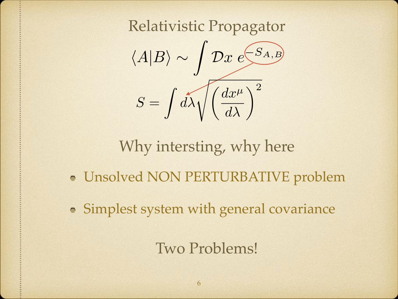
Relativistic Propagator
hA|Bi ⇠Z
Dx e
�SA,B
Two Problems!
S =
Zd�
s✓dx
µ
d�
◆2
6
Why intersting, why here
Unsolved NON PERTURBATIVE problem
Simplest system with general covariance

Problem 1: Square root
Relativistic Propagator
Horrible integrals & still wrong result
Problem 2: No Chapman Kolmogorov
No probability conservation&
no stepwise construction of PI
hA|Bi =? ⇧i
8><
>:Ni ·
Zd
dxi e
� P
i
�
r(x
µ
i+1�x
µ
i
)2
�2
!9>=
>;
hA|Ci 6=Z
d
dxBhA|BihB|Ci
7
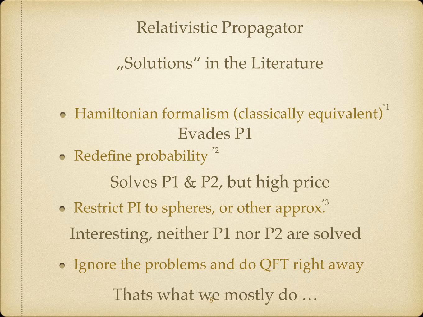
Relativistic Propagator
„Solutions“ in the Literature
Hamiltonian formalism (classically equivalent) Evades P1
Solves P1 & P2, but high price
Interesting, neither P1 nor P2 are solved
Ignore the problems and do QFT right away
Thats what we mostly do …
*1
Redefine probability *2
Restrict PI to spheres, or other approx.*3
8
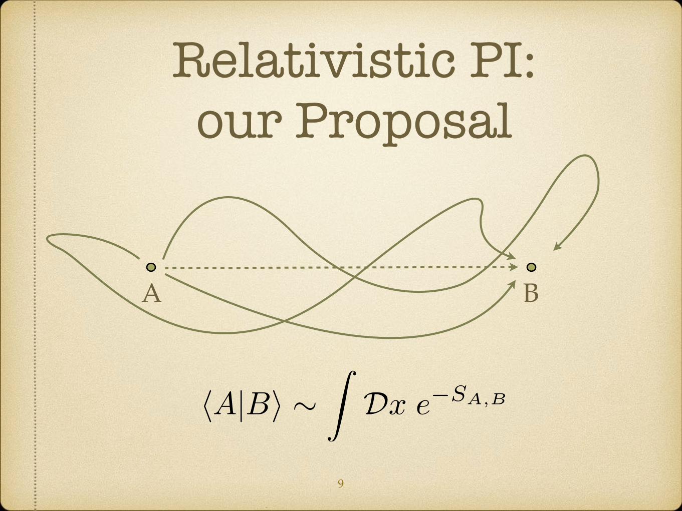
Relativistic PI: our Proposal
A B
hA|Bi ⇠Z
Dx e
�SA,B
9
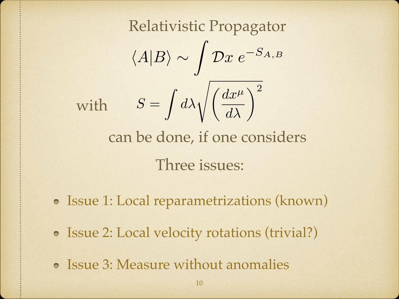
Relativistic Propagator
hA|Bi ⇠Z
Dx e
�SA,B
S =
Zd�
s✓dx
µ
d�
◆2
Issue 1: Local reparametrizations (known)
Issue 2: Local velocity rotations (trivial?)
Issue 3: Measure without anomalies10
with
Three issues:
can be done, if one considers

Relativistic Propagator
hA|Bi ⇠Z
Dx e
�SA,B
S =
Zd�
s✓dx
µ
d�
◆2
11
using I1,I2,I3 works
Functional Fadeev Popov method
*0 Geometricstepwise proof
*00

12
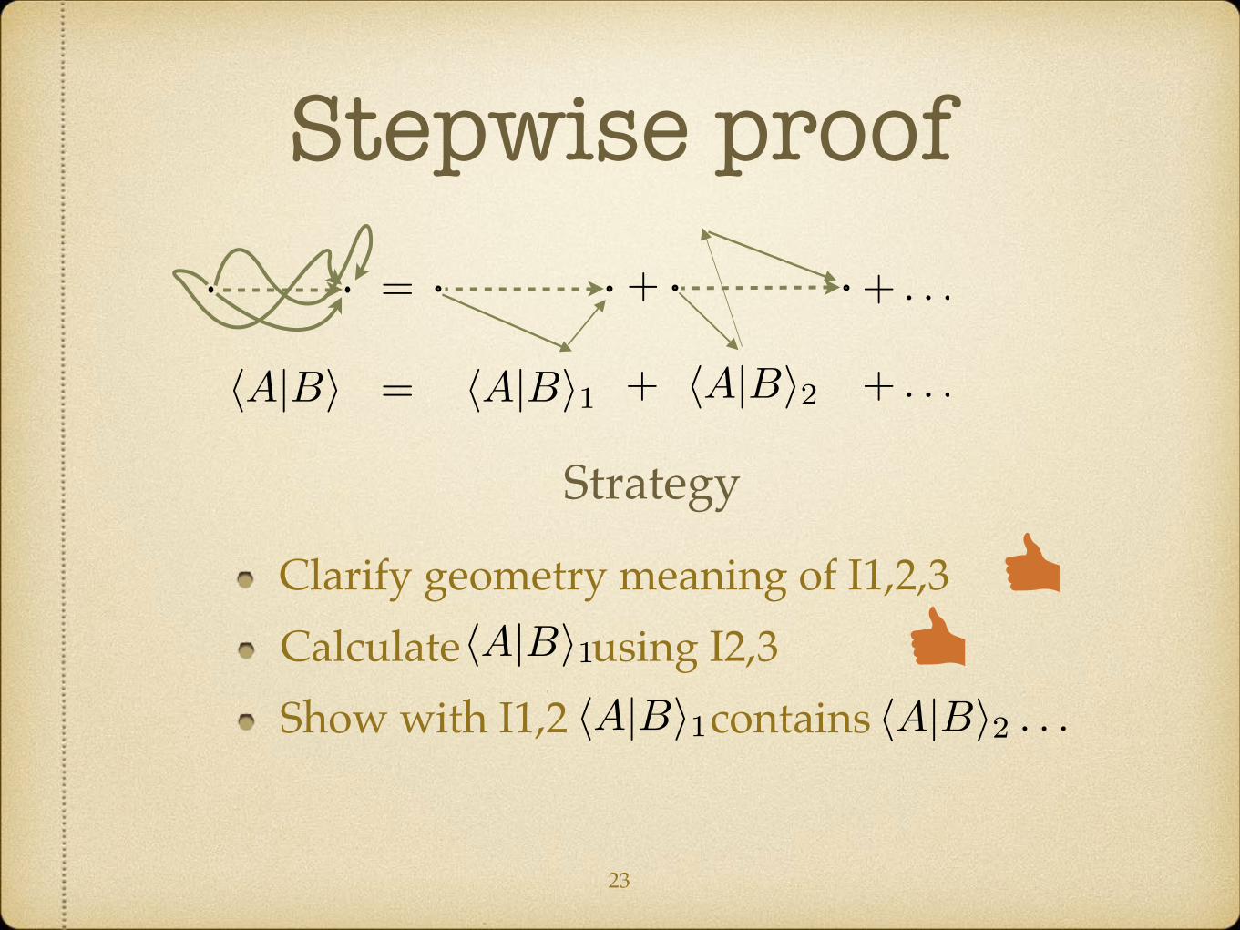
Stepwise proof
A BhA|Bi
=
= hA|Bi1
+ + . . .
hA|Bi2+ + . . .
Strategy
Clarify geometry meaning of I1,2,3Calculate using I2,3 hA|Bi1Show with I1,2 contains hA|Bi2 . . .hA|Bi1
Don’t count again!

S =
Zd�
s✓dx
µ
d�
◆2
13
Issue 1: Local reparametrizations (known)
Invariant under � ! �0(�)
We fix proper time such that
⌧ = ⌧(�)✓dx
µ
d⌧
◆2
= 1with
Geometric over counting:
A B A BC

14
Issue 2: Local velocity rotations (trivial?)
S =
Zd�
s✓dx
µ
d�
◆2
=
Zd�
pv
µvµ
Invariant under vµ ! v0µ = ⇤µ⌫(�)v
⌫
v0µv0µ = vµvµwith
Factor out of PI
. . .. . .
. . .. . .
if and ! S = S0 L = L0

15
Issue 3: Measure without anomalies
When performing transformation
vµ ! v0µ = ⇤µ⌫(�)v
⌫
define right measure invariant under this symmetry:
Dx ! Dx
0 = Dx
Geometric example for two step propagator

16
Stepwise proof
A BhA|Bi
=
= hA|Bi1
+ + . . .
hA|Bi2+ + . . .
Strategy
Clarify geometry meaning of I1,2,3Calculate using I2,3 hA|Bi1Show with I1,2 contains hA|Bi2 . . .hA|Bi1
17
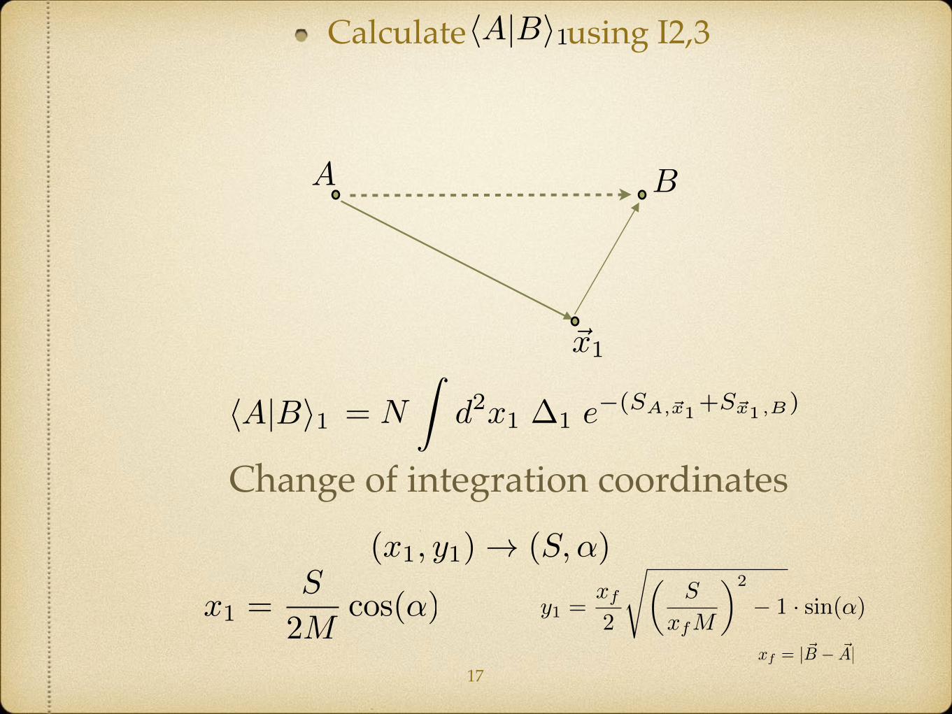
hA|Bi1
~x1
A B
Change of integration coordinates
(x1, y1) ! (S,↵)
x1 =
S
2M
cos(↵)
y1 =xf
2
s✓S
xfM
◆2
� 1 · sin(↵)
xf = | ~B � ~
A|
= N
Zd
2x1 �1 e
�(SA,~x1
+S~x1,B
)
Calculate using I2,3 hA|Bi1

18
~x1
A B
Change of integration coordinates
(x1, y1) ! (S,↵)
x1 =
S
2M
cos(↵)
y1 =xf
2
s✓S
xfM
◆2
� 1 · sin(↵)
xf = | ~B � ~
A|
h0, ~xf
i1 = N2,1(ti,f )
Z 1
xfM
dS
Z 2⇡
0d↵ ·�1
2 (S/M)
2 � x
2f
(1 + cos(2↵))
8
p(S)
2 � (x
f
M)
2exp [�S]
↵S
Calculate using I2,3 hA|Bi1

~x1
h0, ~xf
i1 = N2,1(ti,f )
Z 1
xfM
dS
Z 2⇡
0d↵ ·�1
2 (S/M)
2 � x
2f
(1 + cos(2↵))
8
p(S)
2 � (x
f
M)
2exp [�S]
↵S
0 xf
↵ ! ↵0For one sees and L = L0S = S0
I2 velocity rotation!Naive, measure depends on : anomaly I3 ↵
cancels anomaly��11 ⌘ |~x1 � 0| · |~xf � ~x1|
Calculate using I2,3 hA|Bi1
19

↵S
0 xf
↵ ! ↵0For nothing changes
h0, ~xf
i1 = N2,1
✓Z 2⇡
0d↵
◆·Z 1
xfM
dS
1p(S)
2 � (x
f
M)
2exp [�S]
h0, ~xf i1 = N ·K0(xfM)
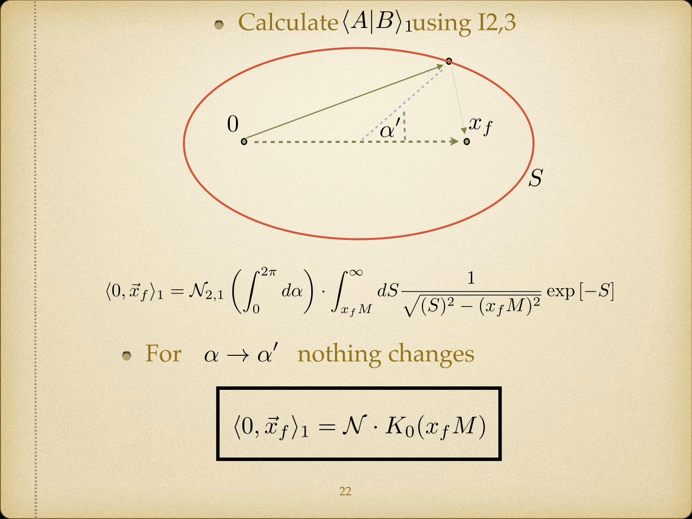
Calculate using I2,3 hA|Bi1
20

S
0 xf
↵ ! ↵0For nothing changes
h0, ~xf
i1 = N2,1
✓Z 2⇡
0d↵
◆·Z 1
xfM
dS
1p(S)
2 � (x
f
M)
2exp [�S]
h0, ~xf i1 = N ·K0(xfM)
↵0
Calculate using I2,3 hA|Bi1
21
S
0 xf
↵ ! ↵0For nothing changes
h0, ~xf
i1 = N2,1
✓Z 2⇡
0d↵
◆·Z 1
xfM
dS
1p(S)
2 � (x
f
M)
2exp [�S]
h0, ~xf i1 = N ·K0(xfM)
↵0
Calculate using I2,3 hA|Bi1
22
23
Stepwise proof
A BhA|Bi
=
= hA|Bi1
+ + . . .
hA|Bi2+ + . . .
Strategy
Clarify geometry meaning of I1,2,3Calculate using I2,3 hA|Bi1Show with I1,2 contains hA|Bi2 . . .hA|Bi1
24
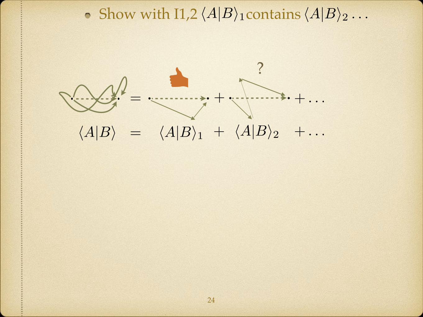
A BhA|Bi
=
= hA|Bi1
+ + . . .
hA|Bi2+ + . . .
Show with I1,2 contains hA|Bi2 . . .hA|Bi1
?
25
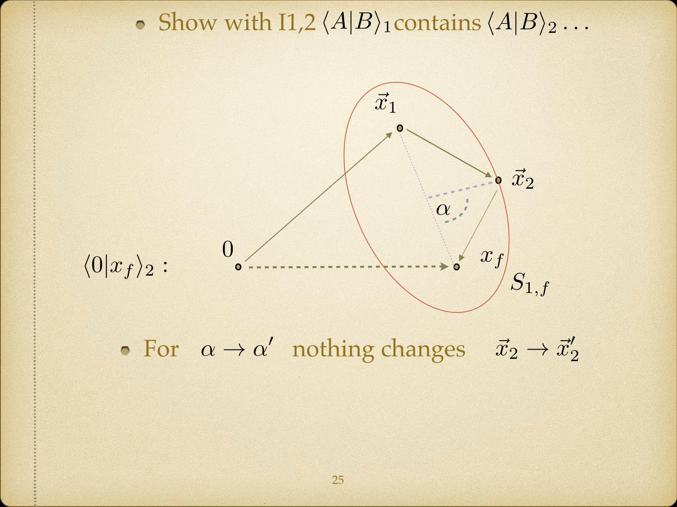
Show with I1,2 contains hA|Bi2 . . .hA|Bi1
0xfh0|xf i2 :
~x1
~x2
↵
S1,f
↵ ! ↵0For nothing changes ~x2 ! ~x
02

26
Show with I1,2 contains hA|Bi2 . . .hA|Bi1
0xf
~x1
h0|xf i2 :S1,f
↵ ! ↵0For nothing changes (I2) ~x2 ! ~x
02
~x
02
↵0
straight line: I1 reparametrizations0 ! ~x1 ! ~x
02
27
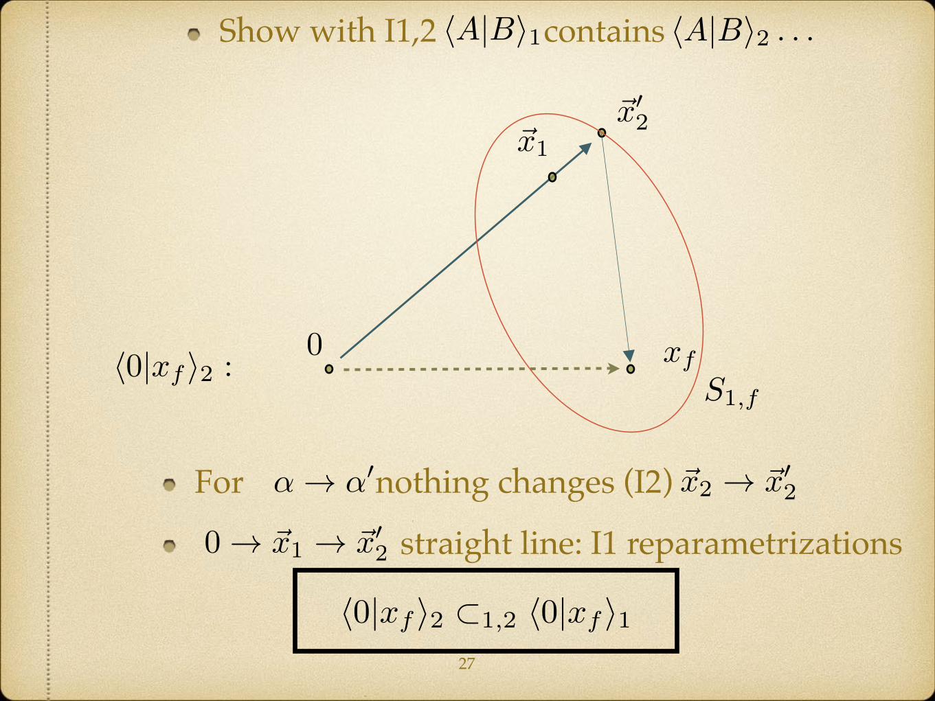
Show with I1,2 contains hA|Bi2 . . .hA|Bi1
0xfh0|xf i2 :
~x1
S1,f
↵ ! ↵0For nothing changes (I2) ~x2 ! ~x
02
~x
02
straight line: I1 reparametrizations0 ! ~x1 ! ~x
02
h0|xf i2 ⇢1,2 h0|xf i1
28
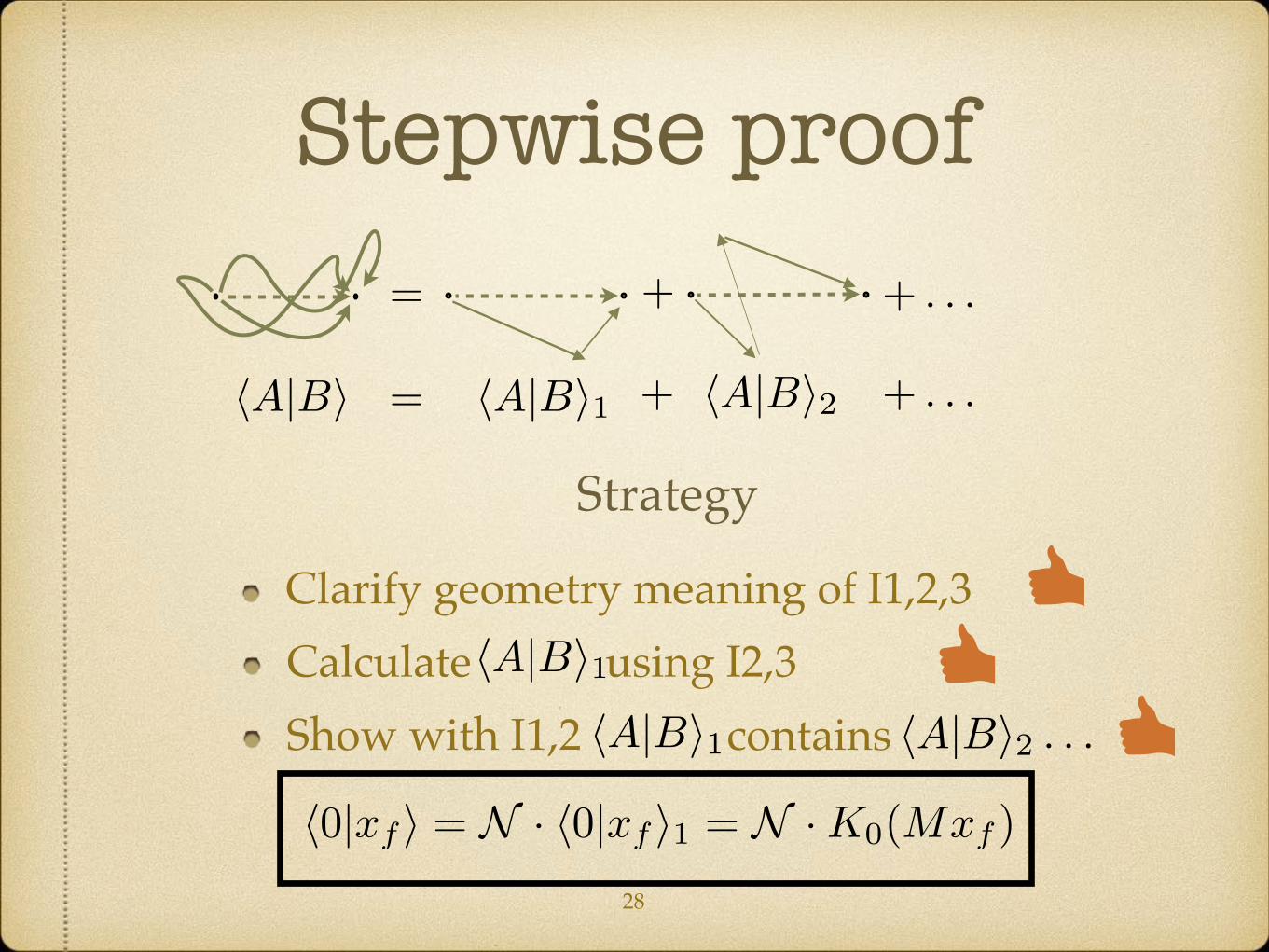
Stepwise proof
A BhA|Bi
=
= hA|Bi1
+ + . . .
hA|Bi2+ + . . .
Strategy
Clarify geometry meaning of I1,2,3Calculate using I2,3 hA|Bi1Show with I1,2 contains hA|Bi2 . . .hA|Bi1
h0|xf i = N · h0|xf i1 = N ·K0(Mxf )

Concluding Comments
Generalization to D dimensions
PI of RPP action can be done, considering I1,I2,I3
Chapman Kolmogorov becomes „trivial“
Future work …
29
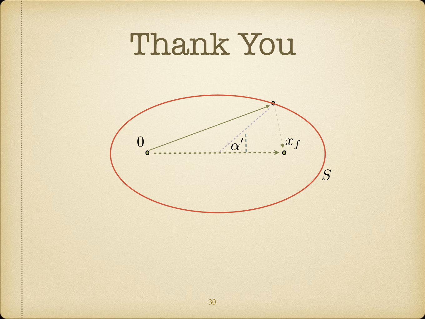
S
0 xf↵0
Thank You
30
Literature
31
0) B. K., E. Muñoz and I. Reyes; Phys.Rev. D96 (2017) no.8, 08501100) B. K., E. Muñoz; arXiv:1706.05388.1) J. Polchinski, “String Theory”, Cambridge U. P., ISBN 0521-63303-6, page 145.; H. Kleinert, “Path Integrals in Quantum Mechanics…”, World Scientific Publishing, ISBN 978-981-4273-55-8, page 1359–1369. M. Henneaux and C. Teitelboim, Annals Phys. 143, 127 (1982).2) P. Jizba and H. Kleinert, Phys. Rev. E 78, 031122 (2008). 3) E. Prugovecki, Il Nuovo Cimento, 61 A, N.2, 85 (1981). H. Fukutaka and T. Kashiwa, Annals of Physics, 176, 301 (1987). Padmanabhan, T. Found Phys (1994) 24: 1543.


