The problem of sampling error in psychological research

• We previously noted that sampling error is problematic in psychological research because differences observed between experimental conditions could be due to real differences or sampling error.

Example of the problem

• Example: We want to know whether psychotherapy increases people’s psychological well-being. The average well-being of Chicagoans is 3.00 (SD = 1). We give a randomly sampled group of 25 Chicagoans therapy. Months later, we measure their well-being. The average well-being in this sample is 3.50.

Big Question

• Is the .50 difference between the therapy group and Chicagoans in general a result of therapy or an “accident” of sampling error?

• Note: There are two hypotheses implied in this question:– The sample comes from a population in which the mean is 3.00, and

the difference we observed is due to sampling error. (Often called the “null hypothesis.”)

– The sample does not come from a population in which the mean is 3.00. The difference is due to therapy. (Often called the “research hypothesis” or “alternative hypothesis.”)

• How can we determine which of these hypotheses is most likely to be true?

• The most popular tools for answering this kind of question are called Null-Hypothesis Significance Tests (NHSTs).

• Significance tests are a broad set of quantitative techniques for evaluating the probability of observing the data under the assumption that the null hypothesis is true. This information is used to make a binary (yes/no) decision about whether the null hypothesis is a viable explanation for the study results.

Basic Logic of NHST

• If we assume the null hypothesis is true (e.g., the difference between our sample mean and the population mean is due to sampling error), then we can generate a sampling distribution that characterizes the the distribution of sample means we might expect to observe.

• That is, if we make certain assumptions about the population (e.g., mu = 3) and the sampling process (e.g., random sampling, N = 25), we can determine (a) the expected sample mean and (b) the expected difference between an observed sample mean and the population mean when a sampling error is made.

• If the probability of observing our sample mean under these assumptions is “small,” we reject the null hypothesis.

• If the probability of observing our sample mean under these assumptions is “large,” we accept the null hypothesis.

WELL-BEING

1 2 3 4 5

Distribution of well-being in the population ( = 3, = 1)

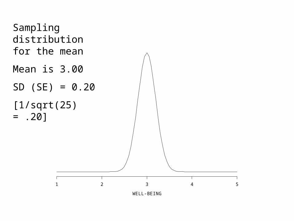
Sampling distribution for the mean

Mean is 3.00

SD (SE) = 0.20

[1/sqrt(25) = .20]

WELL-BEING

1 2 3 4 5

WELL-BEING

1 2 3 4 5

Recall that we can find the proportion of sample means that fall between specific values.

We can interpret these as probabilities in the relative frequency sense of the term.

34%

14%

2 %

• *** We can use these probabilities to determine how likely it is that we will observe a range of sample means based on sampling error alone. Note: This is the same logic we used when we constructed confidence intervals in the last lecture. ***

• In our example, the probability of observing a sample mean between 2.8 and 3.2 is 68%.

• The probability of observing a sample mean equal to or greater than 3.5 is approximately 1%.

How NHSTs work

• Is 1% a “small” probability?• Because the distribution of sample means is continuous,

we must create an arbitrary point along this continuum for denoting what is “small” and what is “large.”

• By convention, if the probability of observing the sample mean is less than 5%, researchers reject the null hypothesis.

WELL-BEING

1 2 3 4 5

The probability of observing a mean of 3.5 or higher is less than 5%.

M = 3.5

Rules of the NHST Game

• This probability value is often called a p-value or p.• When p < .05, a result is said to be “statistically

significant”• In short, when a result is statistically significant (p < .05),

we conclude that the difference we observed was unlikely to be due to sampling error alone. We “reject the null hypothesis.”

• If the statistic is not statistically significant (p > .05), we conclude that sampling error is a plausible interpretation of the results. We “fail to reject the null hypothesis.”

• It is important to keep in mind that NHSTs were developed for the purpose of making yes/no decisions about the null hypothesis.

• As a consequence, the null is either accepted or rejected on the basis of the p-value.

• For logical reasons, some people are uneasy “accepting the null hypothesis” when p > .05, and prefer to say that they “failed to reject the null hypothesis” instead. – This seems unnecessarily cumbersome to me, and divorces the

technique from its original decision-making purpose.

– In this class, please feel free to use whichever phrase seems most sensible to you.

Points of Interest

• The example we explored previously was an example of what is called a z-test of a sample mean.

• Significance tests have been developed for a number of statistics

– difference between two group means: t-test

– difference between two or more group means: ANOVA

– differences between proportions: chi-square

• We’ll discuss some common problems and misinterpretations of p-values and NHSTs in two weeks, but, for now, there are a few of things that you should bear in mind in the meantime:

– (1) The term “significant” does not mean important, substantial, or worthwhile.

• (2) The null and alternative hypotheses are often constructed to be mutually exclusive. If one is true, the other must be false.

• As a consequence, – When you reject the null hypothesis, you accept the alternative.– When you accept the null hypothesis, you reject the alternative.

• This may seem tricky because NHSTs do not test the research hypothesis per se. Formally, only the null hypothesis is tested.

• In addition, the logical problems discussed previously are relevant here.

• (3) Because NHSTs are often used to make a yes/no decision about whether the null hypothesis is a viable explanation, mistakes can be made.

Null is true Null is falseN

ull i

s tr

ueN

ull i

s fa

lse

Real WorldC

oncl

usio

n of

the

test

Correct decision

Correct decision

Type II error

Type I error

Inferential Errors and NHST

Errors in Inference using NHST

• Type I error: Your test is significant (p < .05), so you reject the null hypothesis, but the null hypothesis is actually true.

• Type II error: Your test is not significant (p > .05), you don’t reject the null hypothesis, but you should have because it is false.

• The probability of making a Type I error is determined by the experimenter. Often called the alpha value. Usually set to 5%.

• The probability of making a Type II error is determined by the experimenter. Often called the beta value. Usually ignored by researchers.

Errors in Inference using NHST

Errors in Inference using NHST

• The converse of Type II error is called Power: the probability of rejecting the null hypothesis when it is false—a correct decision. 1- beta

• Power is strongly influenced by sample size. With larger N, more likely to reject null if it is false.

• Note: N does not influence the likelihood of making a correct decision if the null hypothesis is true (i.e, not rejecting null). This probability is always equal to 1-alpha, regardless of sample size.