
University at Albany, State University of New York University at Albany, State University of New York
Scholars Archive Scholars Archive
Business/Business Administration Honors College
5-2017
The Relationship Between Defense Expenditures and Economic The Relationship Between Defense Expenditures and Economic
Growth: A Granger Causality Approach Growth: A Granger Causality Approach
Colin Manchester University at Albany, State University of New York
Follow this and additional works at: https://scholarsarchive.library.albany.edu/honorscollege_business
Part of the Business Commons
Recommended Citation Recommended Citation Manchester, Colin, "The Relationship Between Defense Expenditures and Economic Growth: A Granger Causality Approach" (2017). Business/Business Administration. 37. https://scholarsarchive.library.albany.edu/honorscollege_business/37
This Honors Thesis is brought to you for free and open access by the Honors College at Scholars Archive. It has been accepted for inclusion in Business/Business Administration by an authorized administrator of Scholars Archive. For more information, please contact [email protected].

1
The Relationship between Defense Expenditures
and Economic Growth: A Granger Causality
Approach
Colin Manchester
Abstract
This paper examines the relationship between defense spending and economic growth in the
United States of America between 1947 and 2016. Using quarterly data from the Federal Reserve
of St. Louis Economic Data and the Granger Causality methodology, this study examines the
potential two-way causality between defense spending and economic growth. The results suggest
that over the longer time span of 6-7 years, Granger Causality was not seen between defense
spending and economic growth. However, while analyzing incremental periods in smaller
sections, there were differing findings about the nature of causality.

2
Introduction
This paper will take a look at the relationship between defense expenditure and economic
growth. There has been extensive research conducted in economies in Europe, South America,
and emerging BRIC countries, but there is a clear lack of causal research done on the United
States (Dash & Sahoo 2016, Peacock & Wiseman 1961). There are multiple ways of determining
a causal relationship between defense expenditure and economic growth including Vector Auto
regression (VAR), Structural Vector Auto regression (SVAR), Granger Causality, and more. In
this paper, Granger Causality will be the primary method to determine the two-way causality
between defense expenditure and economic growth in the United States. Some studies in this
field have often found that there is a two-way relationship between defense expenditure and
economic growth, meaning that defense spending Granger causes economic growth and vice-
versa. The time series analysis will take the years 1947 to 2016 as the range of the data sample.
It is important to study the relationship between defense expenditure and economic growth in the
United States because the United States has the largest defense expenditure in the world and
surprisingly little empirical research has been conducted on this specific two-way relationship in
the U.S. in recent years.
Literature Review
This paper will look at the relationship between the nature of defense spending on the
economic well-being of the United States proxied by Defense Consumption Expenditures and
Gross Investment, and Real GDP per Capita. It is a commonly held belief that defense spending

3
has a relationship to economic growth. This stems from Keynes’ (1937) study on fiscal policy.
Keynes found that short run economic growth was caused by the mobilization of resources, such
as defense spending. However, it should be noted that there are other theories as well. Peacock &
Wiseman (1961) looked into the Wagnerian theory suggesting that the opposite may be true.
Under the Wagnerian theory, a period of economic growth would actually then spur the amount
of capital generated as a nation, allowing for more capital to be spent on defense. This paper will
look at the lagging and leading variables to determine the direction of the relationship between
defense spending and short run economic growth.
Evidence of a positive relationship between Defense Spending and Economic Growth
This field of study originated in Benoit’s (1973) paper observing the relationship between
defense expenditure and economic growth in developing countries. Benoit found that there was a
positive relationship between the two variables. The data showed that if a country had a high
military burden, it had a rapid rate of growth. According to his analysis, there was less than a 1-
in-1000 chance that these findings were accidental. He used Spearman correlation, and then
confirmed his findings with regression analysis.
Dash et al (2016) focused their study on the relationship between defense spending and
economic growth in the BRIC countries. Their study shows that in the BRIC countries, a 1% rise
in GDP has been associated with a 0.54% rise in real defense expenditure per capita. Using panel
data and Dynamic Ordinary Least Squares (DOLS), they showed that a 1% increase in economic
growth is associated with a 0.86% increase in real defense expenditure. This study gave a
percentage based look into the positive relationship between defense spending and economic
growth.

4
Owyang et al (2013) discussed the differences in government spending multipliers during
periods of slack in Canada and the United States. Using the local projection method and
quarterly data from 1980 to 2010, they found that there was no evidence that multipliers are
higher in the United States. However, using quarterly data from 1921 to 2010 for Canada, there
was evidence that the government spending multipliers were greater during times when resources
were idle and the economy was operating at less than full employment and equilibrium output.
Evidence of negative relationship between Defense Spending and Economic Growth
On the other hand, Deger and Smith (1983), found a negative relationship between the
two variables in developing countries. This study comprised 44 Less Development Countries
(LDCs). They note that when a developing country is increasing its defense spending, it diverts
resources away from other possible avenues, such as investment. Also, they note that if the
military demands a specific product, there is a possibility that there will be more firms
attempting to generate that item, causing a surplus. Their study concluded that defense spending
had a small positive effect on growth, but had a large negative effect on savings. Therefore, they
concluded that the net effect of increased military spending on economic growth was negative.
Ward and David (1992) conducted research on the United States from 1948 to 1996
examining the relationship between military expenditures and economic growth. Their study
found that the military expenditures actually had a negative relationship with economic growth.
This could be due to the fact that the amount of money spent on the military may have been more
productively employed elsewhere. Both military and non-military government spending have
lower “factor productivity” compared to the private sector, meaning that the private sector is

5
more efficient in the way it uses its resources. However, they do note that there are clear spin-off
benefits generated by increased military spending.
Non-determinant evidence
Several studies have shown that there is no general consensus as to whether there is a
causal relationship between defense spending and economic growth in either direction. Dakurah
et al (2001) showed that in the survey of 62 developing countries, there are 20 countries that
show a Granger Causality from defense spending to economic growth, implying that Keynesian
economic theory is at work in the associated country. However, 17 countries showed exactly the
opposite, with Granger Causality from economic growth to defense spending. This shows that
Wagnerian theory was actually the prevalent economic theory. In addition to the unidirectional
causality, there were also 7 countries with two-way causality, which means that economic
growth causes a change in defense spending, but defense spending causes a change in economic
growth as well.
Ozun & Erbaykal (2014) examined the causal relationship between defense spending and
economic growth. They concluded that there were unilateral causal relationships in 7 NATO
countries, while five countries were found to have no causal relationship at all. Turkey was the
sole country in the data sample that showed a two-way causal relationship between defense
spending and economic growth. Yildirim and Öcal (2006) looked at the conflict between
Pakistan and India and the effects of the extra militarization and arms race conflict on economic
growth. Their findings were that there was a Granger causal relationship between defense
spending and economic growth in India, but not in Pakistan. To further look into the nature of

6
this relationship, they used a VAR analysis to conclude that this increased defense spending
primarily spurred short run economic growth, but not long term economic growth.
Dudzeviciute et al (2016) took an in depth look at the different levels of economic
development, and how that influenced the relationship between defense spending and economic
growth. Their study focuses on five different levels of economic development. Low economic
level, lower middle economic level, upper middle economic level, high economic level, and very
high economic level comprise the categories. It is important to note that this data ranged from
2004 to 2013, so the financial crisis definitely played a role in the economic landscape of all of
the countries in this study. Interestingly, the largest drops in GDP per capita came from the low
economic level and the very high economic level groups. As far as interrelationship is concerned,
all but the lower middle economic level showed a negative relationship between economic
growth and defense spending. This implies that the higher the economic growth, the less is spent
on defense spending.
United States defense expenditure
Harrison (2016) analyzes the fiscal year of 2017’s defense budget. Out of the $905 billion
budget, $523.9 billion is requested for the Department of Defense’s base budget. This does not
include things like military veterans’ health insurance. There are some interesting data points
discussed throughout this study. For instance, during the Korean war, the defense budget grew
more than fivefold in three years. Also, before defense spending became heavily technological,
there was a strong pattern of defense spending rising and falling with the amount of troops
physically deployed. However, following Ronald Reagan’s term as Commander in Chief,
physical deployment of troops were not the main component of defense spending. This analysis

7
was not used for any hard data analysis in this study, but it was interesting to see what the United
States Military budget is broken into.
Granger Causality
With respect to methodology, Granger (1969) looked at a two-variable case to establish a
link between relationship and causality. He found that a feedback mechanism can be treated as
two causal mechanisms joined. This work later led into what is known as a Granger Causality.
Granger testing in Dudzeviciute et al (2016) shows that there is an absence of Granger Causality
between defense spending and GDP per capita in high economic level countries, upper middle
level countries, and low economic level countries. Based on this paper, we would expect to see
that in the United States, increased defense spending would mean less economic growth.
Dudzeviciute’s study is limited in its decision to use only two variables, GDP per capita and
defense spending.
In this paper, a Granger Causality analysis will be used to determine causality. Granger
Causality is appropriate to use in a one to one relationship, and for a time series analysis it will
be an appropriate test to use.
Hypothesis
The null hypothesis for this study (H0) is that defense spending does not Granger Cause
economic growth, nor does economic growth Granger Cause defense spending. This implies that
the two are independent from one another. The alternative hypothesis (H1) is that defense

8
spending Granger Causes economic growth, and that economic growth Granger Causes defense
spending.
Data and Sample
The sample used in this study includes the time period from 1947 to 2016. Quarterly data
are collected from the Federal Reserve Economic Data at the St. Louis Fed (FRED). FRED data
contains the National Defense Consumption Expenditures and Gross Investment as well as the
Real GDP per Capita.
Methodology
The purpose of this paper is to determine the degree of causality between defense
expenditure and economic growth. This will be done through Granger Causality testing similar to
that used in Dudzeviciute et al (2016). Granger testing is the process of using one series of data,
analyzing its movements, then determining if it predicts the later movements of a different series
of data. Therefore, this research will first see if defense spending Granger Causes economic
growth, and then see if economic growth Granger Causes defense expenditure. It is important to
note that the two are not mutually exclusive. As shown before in Ozun & Erbaykal (2014),
Granger testing can show two-way causality between two variables. It is also important to note
that it can show one-way causation, or no causation at all. Granger Causality requires two
separate equations to determine causality as shown in multiple previous research studies
(Farzanegan, 2014; Mosikari & Matlwa,2014). The regression equations below are used to
determine Granger Causality in this paper.

9
𝑌" = 𝛽&,( + 𝛽&,* 𝑌"+*
,
*-&
+ 𝛽&,,./ 𝑋"+/
,
/-&
+ 𝜀&"
𝑋" = 𝛽2,( + 𝛽2,* 𝑌"+*
,
*-&
+ 𝛽2,,./ 𝑋"+/
,
/-&
+ 𝜀2"
β parameters to be estimated, ϵ error, p is the number of lags used.
These regression equations show the effect of one variable on the other in terms of a
lagged structure. A variable can be said to Granger Cause another when lagged values of “x” can
assist in forecasting the current state of “y”, as long as all other relevant information is given
(Stern 2011). For purposes of this study, Y is the log of National Defense Consumption
Expenditures and Gross Investment (defense spending) and X is the log of Real GDP per Capita
(economic growth).
All calculations have been analyzed using Eviews econometric software.
Time Series Analysis of Defense Spending and Economic Growth
Investigating the years 1947-2016, there are significant trends to identify concerning both
defense spending and economic growth.

10
Exhibit 1
As seen in Exhibit 1, from 1988 to 1999, defense expenditure as a total percentage of
GDP fell from 5.7% to just below 3%. Following 1999, defense expenditure as a total percentage
of GDP then rose until 2010 to 4.7%, from which point it fell to 3.3% in 2015. In the same
exhibit, we can see the rise and fall of the annual GDP growth rate. While defense expenditure as
a proportion of GDP moved along a relatively smooth path, annual GDP growth rate had very
volatile changes. First, from 1988 to 1990, the annual GDP growth rate fell from 4.2% to -.07%,
then immediately rebounded to 4.7% the following year. Another large drop is seen from 2000 to
mid-2001, which could possibly be explained by the Dot-com bubble bursting in March, 2000.
-‐4.0%
-‐3.0%
-‐2.0%
-‐1.0%
0.0%
1.0%
2.0%
3.0%
4.0%
5.0%
6.0%
7.0%
1988
1989
1990
1991
1992
1993
1994
1995
1996
1997
1998
1999
2000
2001
2002
2003
2004
2005
2006
2007
2008
2009
2010
2011
2012
2013
2014
2015
Defense Spending as % of GDP & Annual GDP Growth Rate
% share of GDP Annual GDP Growth Rate

11
The most striking point in this data though is the enormous drop from mid-2007 to mid-2009
following the financial crisis. Already falling annual GDP growth rates plummeted from just
below 2% to almost -3%. This shows only the second time in this time period annual GDP
growth rate was negative, and the only time it was more than 0.1% negative.
In accordance with the large drops in annual GDP growth rate, there are differences in the
political atmosphere as well. During the drop from 1989 to 1991, there was a Democratically
controlled Senate, as well as a Democratically controlled House of Representatives, shown by
blue shading. At the time of the Dot-com bubble burst, there was a Republican controlled Senate,
and a Republican controlled House of Representatives, shown by red shading. Out of all
significant drops during this time period, the Financial Crisis was the largest. At this time, there
was a split Senate, and a Democratically controlled House of Representatives. This information
is interesting to see, because Congress is responsible for passing the laws associated with a
majority of fiscal decisions, as well as taxation plans. It is important to note that there were large
drops in annual GDP growth rate regardless of whether or not it was a Republican or
Democratically controlled Congress.

12
Exhibit 2
Exhibit 2 shows both the defense expenditure per capita and defense expenditure in total
USD. Starting with defense expenditure, from 1988 to 2014 it has risen 103% from $293 billion
to $596 billion. However, defense expenditure peaked in this time period in 2011 at $711 billion
dollars. Looking at defense expenditure per capita, there is an almost identical graph due to the
fact that the large amount of capital spent on defense expenditure dwarfs the relatively small
amount of change in people. From 1988 to 2015, defense expenditure per capita has increased
55% from $1,196 to $1,854. Again it peaked in 2011 at $2,279.
$-‐$100 $200 $300 $400 $500 $600 $700 $800
1988
1990
1992
1994
1996
1998
2000
2002
2004
2006
2008
2010
2012
2014
Billion
s
Defense Spending
$-‐
$500
$1,000
$1,500
$2,000
$2,500
1988
1990
1992
1994
1996
1998
2000
2002
2004
2006
2008
2010
2012
2014
Defense Spending per Capita

13
Exhibit 3
Exhibit 3 shows both the United States’ GDP and GDP per capita. Similar to Exhibit 2,
these graphs look nearly identical. U.S. GDP increased from $5.2 trillion to $17.9 trillion from
1988 to 2015, a 242% rise. GDP per capita has risen 160% from $21,483 to $55,836 during the
same time period. Although Exhibit 2 shows a more warped graph, both GDP per capita and
GDP have seen close to a linear relationship in accordance with the time period, excluding a
bump and fall from 2006 to 2008.
$-‐$2 $4 $6 $8 $10 $12 $14 $16 $18 $20
Trillions
U.S. GDP
$-‐
$10,000
$20,000
$30,000
$40,000
$50,000
$60,000
1988
1992
1996
2000
2004
2008
2012
U.S. GDP per Capita
14
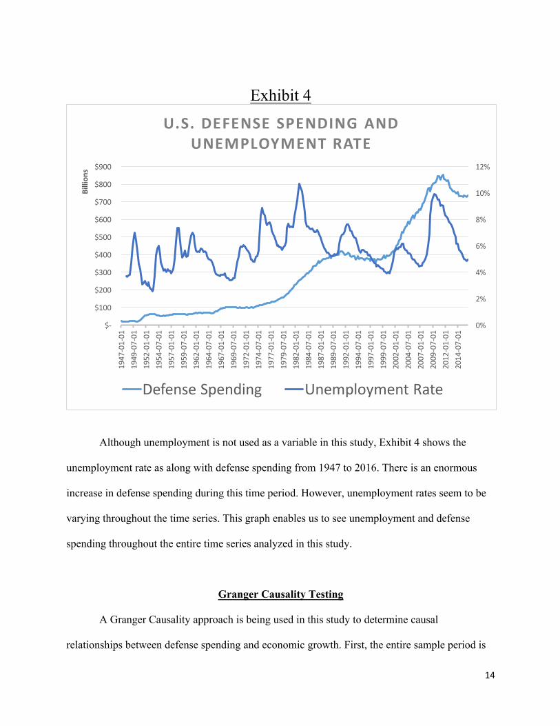
Exhibit 4
Although unemployment is not used as a variable in this study, Exhibit 4 shows the
unemployment rate as along with defense spending from 1947 to 2016. There is an enormous
increase in defense spending during this time period. However, unemployment rates seem to be
varying throughout the time series. This graph enables us to see unemployment and defense
spending throughout the entire time series analyzed in this study.
Granger Causality Testing
A Granger Causality approach is being used in this study to determine causal
relationships between defense spending and economic growth. First, the entire sample period is
0%
2%
4%
6%
8%
10%
12%
$-‐
$100
$200
$300
$400
$500
$600
$700
$800
$900
1947-‐01-‐01
1949-‐07-‐01
1952-‐01-‐01
1954-‐07-‐01
1957-‐01-‐01
1959-‐07-‐01
1962-‐01-‐01
1964-‐07-‐01
1967-‐01-‐01
1969-‐07-‐01
1972-‐01-‐01
1974-‐07-‐01
1977-‐01-‐01
1979-‐07-‐01
1982-‐01-‐01
1984-‐07-‐01
1987-‐01-‐01
1989-‐07-‐01
1992-‐01-‐01
1994-‐07-‐01
1997-‐01-‐01
1999-‐07-‐01
2002-‐01-‐01
2004-‐07-‐01
2007-‐01-‐01
2009-‐07-‐01
2012-‐01-‐01
2014-‐07-‐01
Billion
s
U.S. DEFENSE SPENDING AND UNEMPLOYMENT RATE
Defense Spending Unemployment Rate

15
analyzed, going up to 28 lags, or 7 years. Second, the data will be analyzed in specific sub-
sample periods to determine if the findings change depending on the time period studied. All
data are collected through the Federal Reserve Economic Data, and consist of quarterly data
from 1947 to 2016. In order to linearize the data series, this study analyzes the log of both
defense spending and economic growth in the Granger Causality testing. The results are
presented in Tables 1 and 2 below.
Table 1
Long term Granger Causality Testing
As shown above, between 1947 and 2016, the null hypothesis that GDP per capita does
not Granger Cause defense spending, and that defense spending does not Granger Cause GDP
Lags Null(Hypothesis Observations F7Statistic Probability Test(Results
4GDP%per%Capita%does%not%Granger%Cause%Defense%Spending
2753.2429 0.0128 Reject
Defense%Spending% does% not%Granger%Cause%GDP%per%Capita% 2.8386 0.0248 Reject
8GDP%per%Capita%does%not%Granger%Cause%Defense%Spending
2712.60189 0.0095 Reject
Defense%Spending% does% not%Granger%Cause%GDP%per%Capita% 2.66268 0.008 Reject
12GDP%per%Capita%does%not%Granger%Cause%Defense%Spending
2671.97354 0.0273 Reject
Defense%Spending% does% not%Granger%Cause%GDP%per%Capita% 1.95763 0.0288 Reject
16GDP%per%Capita%does%not%Granger%Cause%Defense%Spending
2631.53343 0.0893 Reject
Defense%Spending% does% not%Granger%Cause%GDP%per%Capita% 1.92686 0.0191 Reject
20GDP%per%Capita%does%not%Granger%Cause%Defense%Spending
2591.86361 0.0162 Reject
Defense%Spending% does% not%Granger%Cause%GDP%per%Capita% 1.75276 0.0274 Reject
24GDP%per%Capita%does%not%Granger%Cause%Defense%Spending
2551.63623 0.0362 Reject
Defense%Spending% does% not%Granger%Cause%GDP%per%Capita% 1.84353 0.0124 Reject
28GDP%per%Capita%does%not%Granger%Cause%Defense%Spending
2511.33798 0.1306 Fail(to(Reject
Defense%Spending% does% not%Granger%Cause%GDP%per%Capita% 1.49923 0.0599 Reject

16
per capita can be rejected up to 24 lags, or 6 years. This means that there is statistically
significant evidence that one of these variables can be used to predict the level of the other up to
six years. It is important to note that in the 28 lag structure, or 7 years, that the null hypothesis
that GDP per capita does not Granger Cause defense spending can be rejected. As shown, the 8
lag structure tests provide high F-statistics which correlates with a 1% confidence interval. The
4, 12, 16, 20, and 24 lag structure tests all are within 10% confidence, with every test excluding
“GDP per Capita does not Granger Cause Defense Spending” in the 16 lag structure within a 5%
confidence level.
Table 2
Sub-Period Granger Causality Testing
Time%period Null%Hypothesis Observations F8Statistic Probability Test%Results
1947Q1& ' 1955Q4
GDP&per&Capita&does¬&Granger&Cause&Defense&Spending
28
1.93094 0.1542 Fail%to%Reject
Defense&Spending&does¬&Granger&Cause&GDP&per&Capita& 1.33179 0.322 Fail%to%Reject
1956Q1& ' 1970Q4
GDP&per&Capita&does¬&Granger&Cause&Defense&Spending
48
1.22257 0.3263 Fail%to%Reject
Defense&Spending&does¬&Granger&Cause&GDP&per&Capita& 2.39483 0.0347 Reject
1971Q1& ' 1984Q4
GDP&per&Capita&does¬&Granger&Cause&Defense&Spending
48
1.50854 0.1915 Fail%to%Reject
Defense&Spending&does¬&Granger&Cause&GDP&per&Capita& 1.24087 0.3157 Fail%to%Reject
1985Q1& ' 2000Q4
GDP&per&Capita&does¬&Granger&Cause&Defense&Spending
48
2.21462 0.049 Reject
Defense&Spending&does¬&Granger&Cause&GDP&per&Capita& 1.40972 0.231 Fail%to%Reject
2001Q1& ' 2016Q3
GDP&per&Capita&does¬&Granger&Cause&Defense&Spending
51
1.5611 0.1654 Fail%to%Reject
Defense&Spending&does¬&Granger&Cause&GDP&per&Capita& 3.48501 0.0037 Reject

17
In the sub-sample testing, there are some interesting changes. During the time periods
from 1947 – 1955 and 1971 – 1984 there was no statistically significant evidence to support the
claim that either of the null hypotheses can be rejected. However, there are some indications of
significance in the other time periods. In both the time periods of 1956 – 1970 and 2001 – 2016
there is statistically significant evidence for rejecting the null hypothesis that defense spending
does not Granger Cause GDP per capita. This implies that during these periods, defense spending
can help predict a pattern in the future value of GDP per capita. Finally, between 1985 – 2000,
the null hypothesis that GDP per capita does not Granger Cause defense spending can be
rejected. In contrast to the previous time periods, during this sample period, GDP per capita can
be used to assist in predicting a pattern in future defense spending.
Conclusions
In this paper, Granger Causality testing has been used to analyze the relationship between
defense spending and economic growth in the United States between 1947 to 2016.
Examining the entire sample period, there was definite statistically significant data that
rejected both null hypotheses. During the whole sample GDP per capita Granger Causes defense
spending and defense spending Granger Causes GDP per capita up to six years. This implies a
two-way causal relationship between the two variables. This is consistent with both Keynesian
and Wagnerian Macroeconomic theories. This two-way causal relationship is consistent with the
7 countries in the Dakurah et al (2001) study. However, when broken down into shorter time
spans, this changes. Different time series lengths saw significantly different results. It would be
very interesting to further research why the shorter time series varied from the entire sample
period. It would be beneficial to further see the short run implications to better allocate funding,

18
especially in times of economic recession. The ability to spur short run growth in these times is
critical. Also, on a long run scale, it would show if defense spending is the correct avenue to
allocate capital to. Perhaps long run economic growth would be better spurred by investment in
health care or infrastructure. Implications of this causal nature shows that it is beneficial to
research this topic further.
There are definite limitations to this paper’s findings. Only defense spending and
economic growth have been used to determine the relationship between one another. Other
outside variables were not considered in this study except to deflate the series. There are a
number of economic factors that play into economic growth, and using a bivariate approach
limits this. Using a Vector Auto Regression would be able to incorporate other outside variables,
such as employment, consumption and income.

19
Works Cited
Benoit, Emile. “Defense and economic growth in developing countries.” (1973). Dakurah, A. Henry, Stephen P. Davies, and Rajan K. Sampath. “Defense spending and economic growth in developing countries: A causality analysis.” Journal of Policy Modeling 23.6 (2001): 651-658. Dash, D. P., Bal, D. P., & Sahoo, M. (2016). Nexus between defense expenditure and economic growth in BRIC economies: An empirical investigation. Theoretical & Applied Economics, 23(1), 89-102. Deger, Saadet, and Ron Smith. (1983) “Military expenditure and growth in less developed countries.” Journal of conflict resolution 27.2: 335-353. Dudzeviciute, G., Peleckis, K., & Peleckiene, V. (2016). Tendencies and Relations of Defense Spending and Economic Growth in the EU Countries. Engineering Economics, 27(3), 246-252. Farzanegan, Mohammad Reza. (2014) “Military spending and economic growth: the case of Iran.” Defence and Peace Economics 25.3: 247-269. Granger, Clive WJ. (1969) “Investigating causal relations by econometric models and cross-spectral methods.” Econometrica: Journal of the Econometric Society: 424-438. Harrison, T. (2016). Analysis of the FY 2017 Defense Budget. Rowman & Littlefield. Keynes, John Maynard. (1937) “The general theory of employment.” The Quarterly Journal of Economics: 209-223. Mosikari, Teboho Jeremiah, and Keabetswe Matlwa. (2014) “An analysis of defence expenditure and economic growth in South Africa.” Mediterranean Journal of Social Sciences 5.20: 2769. Ozun, A., & Erbaykal, E. (2014). Further Evidence On Defence Spending and Economic Growth in NATO Countries. Economic Computation & Economic Cybernetics Studies & Research, 48(2), 1-12. Peacock, Alan T., and Jack Wiseman. (1961) “Front matter, The Growth of Public Expenditure in the United Kingdom.” The growth of public expenditure in the United Kingdom. Princeton University Press, 32-0. Pigou, Arthur C. (1936) “Mr. JM Keynes’ General theory of employment, interest and money.” Economica 3.10: 115-132.

20
Ramey, V. A. (2016). Macroeconomic shocks and their propagation (No. w21978). National Bureau of Economic Research. Sims, Christopher A. “Macroeconomics and reality.” Econometrica: Journal of the Econometric Society (1980): 1-48. Stern, David I. (2011) “From correlation to Granger causality.” Crawford School Research Paper 13 Ward, Michael D., and David R. Davis. (1992) “Sizing up the Peace Dividend: Economic Growth and Military Spending in the United States, 1948-1996.” The American Political Science Review, vol. 86, no. 3, pp. 748–755. http://www.jstor.org/stable/1964136. Yildirim, Jülide, and Nadir Öcal. (2006) “Arms Race and Economic Growth: The Case of India and Pakistan” Defence and Peace Economics17.1: 37-45.


![Index [] · ATM’s (automated teller machines) .....814, 1299 Atomic energy defense activities, expenditures . 549 Audio-video equipment (household) industry manufacturing .....1486](https://cdn.vdocument.in/doc/165x107/5f0dcafe7e708231d43c1ce2/index-atmas-automated-teller-machines-814-1299-atomic-energy-defense.jpg)