The Social Impact of Rural-Urban Migration onUrban �Natives�
Xin Meng� Dandan Zhangy
March 13, 2013
Abstract
Chinese cities have continued to accommodate more and more ruralmigrants as millions has moved out of rural areas since the mid 1990s. Ina companion paper we examined the impact of rural-urban migration onurban native workers�labour market outcomes (employment and wages).This paper examines its impact on urban natives� social outcomes. Inparticular, we are interested in the e¤ect of migration on urban crimerate and urban natives�access to social services. We �nd that rural mi-grants do not impose signi�cant pressures on urban residents�access toeducation and health services, but have a modest negative e¤ect on urbanpublic transportation. With regard to crime we �nd that migrant ratio ispositively associated with urban crime rates. However, the �rst-di¤erenceand �rst-di¤erence with IV estimations result in small negative or zeroe¤ect of migrant ratio on the city crime rate. Thus, the illusion that mi-grants contribute to the increase in the city crime rate is due largely toreverse causality and/or omitted variable biases.
Key word: Migration, Crime, Native social outcomes, China.JEL classi�cation numbers: R23; K42; R28
�Research School of Economics, CBE, Australian National University, Canberra, ACT0200, Australia. Email: [email protected]
yNational School of Development, Peking University, [email protected]
1 Introduction
As a consequence of continuous economic growth in China, the past two decades
has witnessed a rapid city expansion with millions of rural migrants moving from
rural to urban areas. By now, around 150 million rural migrants are working
in Chinese cities with ten to twenty million newcomers each year (NBS, 2009).
This rapid and substantial increase in rural migrant in�ows has aroused great
concerns within city governments and the urban public that rural migrants
might cause social problems in cities, such as imposing pressure on local residents
access to public services and raising crime rates.
A 2008 survey of city community leaders from 19 Chinese cities on attitudes
towards rural migrants suggests that urban residents and local governments are
more concerned with rural migrants social impact than their labour market
impact. Among the 787 urban community heads surveyed, 87 per cent worried
that �rural migrant in�ow threatens the safety and security of local community�.
Furthermore, 67 cent of community heads believed that most of the serious
crime were committed by rural migrants. 58.7 per cent of heads believed rural
migrants �put pressure on social services and city infrastructure�which is much
larger than the proportion concerned that �rural migrants may take jobs away
from urban workers� - which only accounted for 23.4 per cent of community
heads. From urban residents point of view, it seems that rural migrant in�ow
is a major source of city crime and congestion in public infrastructure.
Although the public believes and worries about adverse impact of rural-
urban migrants on city safety and city social services, no one has provided
careful studies to establish the link between migration and the increase in crime
or deterioration of social services or social infrastructure. The lack of empirical
evidence, however, did not deter the government from implementing many re-
strictive policies in order to keep migrants out of the urban areas. For example,
rural migrants�children were restricted from entering urban schools; migrant ac-
cess to urban health-care system is very limited; and majority of migrants has
no unemployment insurance or health insurance which are available to urban
local people.
In this paper we examine whether and the extent to which rural-urban mi-
gration a¤ects city crime rate and urban natives�access to social services.
The remainder of this paper is arranged as follows. Section 2 brie�y dis-
cusses the conceptual framework, the channels through which rural migrants
may a¤ect urban residents�access to social services, provides some institutional
1
background, and surveys the literature in related �elds. The estimation strat-
egy and model speci�cations are presented in Section 3. Section 4 describes
the major data sources and provides summary statistics. Empirical results are
reported and discussed in Section 5. Section 6 concludes the paper.
2 Conceptural Framework, Institutional Back-
ground, and Literature
Unlike the urbanisation process in many developed and developing countries,
rural-urban migration in China has been proceeded under a guest-worker scheme
(Du, Gregory and Meng, 2006), whereby individuals from rural areas (with rural
identi�cation card known as rural hukou) can only move to cities temporarily
for work purpose. Migrants are on average young adults and a larger proportion
of them are males. They come to cities for 7 to 8 years to make money and
their hukou status in general cannot be changed (Golley and Meng, 2011). The
de�nition of �migrants�and �urban residents� in this paper, therefore, is very
clear. �Migrants� refer to individuals with rural hukou but residing in cities,
while �urban residents�refer to people with urban hukou and residing in urban
areas.1
2.1 Channels of Rural Migrants�E¤ects
As an important component of the urban society, rural migrants not only gen-
erate demand for goods and services as consumers but also provide tax revenue
as taxpayers. In this context, rural migrant in�ow may a¤ect urban residents�
access to various social services through two channels.
First, as consumers, rural migrants may compete with urban residents for
the consumption of scarce public facilities and services or they may change
the consumption composition of the total city population through a¤ecting de-
mographic characteristics, thereby a¤ecting urban residents� access to social
services. This e¤ect is a direct e¤ect, which can be further decomposed into
the �scale e¤ect� and the �composition e¤ect�. The �scale e¤ect� is associated
with the increases in population in each city due to rural migrant in�ow.2 If
1We also distinguish �urban-to-urban migrants� from �urban residents�. This is identi�edbased on hukou locations. If an individual with an urban hukou but the hukou location is notin the city he/she is residing the person is identi�ed as �urban-to-urban migrants�.
2Based on the censuses and population survey data, rural migrants have increased totalcity population by 4.8%, 8.5% and 14.1% in 1990, 2000 and 2005, respectively.
2

the level of public service is given, rural migrants may compete with urban
residents in obtaining some social services through increasing the total number
of potential consumers. Thus, the e¤ect through this channel is usually nega-
tive. The �composition e¤ect�is associated with structural changes among the
population, which a¤ects urban consumption behaviour due to the di¤erences
in consumption preferences and demographic features between urban residents
and rural migrants. Because the consumption preferences of rural migrants and
urban residents may be di¤erent for various social services, the e¤ect on urban
residents�access to each social outcome through this channel is ambiguous. It
could be zero or negative.
Second, as taxpayers, rural migrants contribute to the rising of local gov-
ernments��scal revenue. If city governments make use of any such additional
tax revenue to provide more public facilities and services through government
investment, urban residents�access to social services may be kept constant or
even increase. This is an indirect channel, or the ��scal e¤ect�, which is usually
positive. Thus, the government agency, as a decision maker, plays a very im-
portant role in determining rural migrants��scal e¤ect on public services. Since
city governments may invest disproportionately across di¤erent public services ,
the possible �scal e¤ect may actually depend on governments�investment pref-
erences.
Combining the above two channels (i.e., direct and indirect channels), it
is clear that the �nal e¤ect of rural-urban migration on access to various so-
cial services of urban residents is ambiguous, which highlights the necessity for
empirical analysis.
2.2 Institutional settings
Below we provide a brie�y discussion about the possible impacts of rural mi-
grants, as consumers of public services, on urban residents�access to education,
health, public transportation, and their possible impact on urban crime rates
based on the current institutional settings in Chinese urban cities.
Education Services: According to an o¢ cial research report (Research Team
of the State Council, 2006), there were 15 million rural migrants�children (who
hold the rural hukou) residing in cities; among them 44 per cent were aged
between 6 and 15 - the age range for compulsory education; an additional 1.5
million migrants� children may move into cities with their parents each year.
This may imply that a large in�ux of rural migrants�children generates a greater
3
demand for urban basic education.
Although rural migrants and their children have continued to move into
cities, it was not until the late 1990s that they were allowed limited access to
local public schools. For a very long time, rural migrants�children were strictly
restricted from entering urban public schools as they did not have local urban
hukou. As a response, migrants set up their own schools with no input from
local governments. Needless to say, the quality of education in migrant schools
are very low.
In March 1998, a document issued by the central government allowed migrant
children to enter limited classes or schools in destination cities for the �rst time,
conditional on them only enrolled in special classes for migrant children in public
schools or enrolled in private migrant schools. If they enrolled in public schools,
they needed to pay extra fees for enrolment and the local governments of migrant
sending regions were required to restrict school aged children from moving to
cities.
A new regulation in 2001 stipulated that destination city governments should
take the responsibility for providing compulsory education to migrant children
rather than the government in the sending areas. This new regulation legally
guarantees children of migrants�entitlement in accessing basic education in host
cities.
Despite the signi�cant progress made in government policies, in reality mi-
grant children�s access to public schools is still very limited. For example, it is
estimated that in Beijing 70% of the migrant children enrolled in migrant schools
(Liu, 2010), while in one of the best migrant-accommodating cities, Shanghai,
there are still 30% migrant children attending migrant schools today and even
when they are enrolled in the local public schools it has been restricted to the
least resourceful ones (Feng and Chen, 2011). In addition, migrant children are
still not allowed access to schools beyond nine-year compulsory education in
cities. As a result, few can continue their formal education in the host cities
and instead a large number of them drop out of school and start working, which
may a¤ect the education attainment of rural migrants�children. The rest have
to return to their rural hometown to continue their senior high school study.
Health-Care Services: The current urban health insurance system was intro-
duced in urban China in 1998. The system, however, restricts to urban hukou
employees only, rural migrants who do not have urban hukou are not covered by
4
the urban health insurance system.3 Although in recent years some attempts4
were made by the central government to include migrants into the urban health
insurance system, up until 2010, the proportion of migrants with urban health
insurance is around 20% (Frijters, Gregory, and Meng, 2011). Migrants are
covered by the New Rural Cooperative Health Insurance (NRCHI) 5 in their
home villages, but NRCHI does not cover their medical expenditure in cities.
In addition, the majority of rural migrants cannot a¤ord any urban commercial
health insurance. Thus, rural migrants generally do not have much access to
the urban health services. When they are seriously ill, they go back to their
rural villages.
Evidence from the �rst-wave of the Rural-Urban Migration in China and
Indonesia project (RUMiCI)6 China survey conducted in 2008 suggests that,
among those rural migrants who had been sick in the past three months (ac-
counting for 14.3 per cent of total rural migrants), only 15.3 per cent went to
a hospital. Of those individuals with serious illness only 30 per cent went to
a hospital, and only 8.2 per cent of those were covered by health city health
insurance. This suggests the impact of rural migrants on health care provided
by cities is unlikely to be signi�cant.
Public Transportation Services: It is widely believed that the rural migrant
in�ow may impose pressure on inner-city transportation through the �scale ef-
fect�. However, previous studies �nd that many rural migrants who are em-
ployed in the construction sector and manufacturing factories usually live in
construction sets or dormitories provided by employers which are either close to
or at their work sites (Research team of the State Council of China, 2006). The
RUMICI survey indicates that 47% of the migrants in 2008 are living in work
places or employer provided nearby accommodations. Thus, the impact of rural
migrant in�ow on inner-city transportation should not be very large.
City Crime Rates: Crime rates are relatively independent of that public fa-
cilities and services. Nevertheless, the government spending on law enforcement
3See the �Decision on Setting Up Urban Workers�Basic Health Insurance System� issuedby the State Council of China in 1998.
4The new Labour and Contract Law was issued in 2008 which aimed at protecting thebasic social welfare of rural migrants.
5The new rural cooperative health insurance system was initiated in October 2002. It hasbeen widely carried out in rural China since 2008 and is planned to cover all rural areas by2010.
6RUMiCI Survey in China has three main samples: the Rural Household Survey of 8000households, the Urban Household Survey of 5000 households, and the Migrant HouseholdSurvey of 5000 households. The survey was conducted annually from 2008 to 2011. Detailedinformation on the survey and the data are available at http://rse.anu.edu.au/rumici/.
5
is an important determinant of crime rates. This is why we study the migra-
tion impact on crime rates together with that on urban resident access to other
public services.
From the point of view of migrants as consumers of the law enforcement
services, there are several reasons to suspect rural migrant in�ow may lead to
an increase in city crime rates. First, according to economic theory whether an
individual commits a crime is related to opportunity cost (Ehrlich, 1973 and
Becker, 1974). In Chinese cities, rural migrants and urban residents may face
di¤erent opportunity costs in committing a crime. Rural migrants usually earn
less than their urban counterparts and are without any social welfare (Meng
and Zhang, 2001; Sheng and Peng, 2005; Du, Gregory and Meng, 2006). Thus,
they may have a relatively low opportunity cost and high return to commit
crime. Second, the majority of rural migrants are males between 18-40, which
is considered the group which is more likely to be engaged in criminal activities
than the rest of the population (Freeman, 1991; Levitt, 1998; Grogger, 1998).7
Third, rural-urban migrant in�ow is associated with an increase in total city
population as well as population density, which is considered one of the key
determinants of a city�s crime level (Glaeser and Sacerdote, 1999).
2.3 Social Services Related Fiscal Arrangement
In our conceptual framework we assumed two roles of migrant workers: as social
service consumers and as contributors. To understand the net impact of migrant
in�ow on urban local residents�access to social services one needs to have some
information on who pays for these services and where the money comes from.
The �rst issue we care about is the divide between the central and local
governments. As our analysis below based predominantly on across city vari-
ations, we would want to make sure that local governments rather than the
central government pay for majority of these services. Otherwise, in the case of
cross-subsidy, the role of migrants within each city will be very unclear.
China�s �scal arrangement has changed a few times over the past 50 or so
years. The most recent changes occurred in 1984 and 1993. The �rst reform
decentralized the government �scal revenue and spending and increased the
local government role signi�cantly. The 1993 reform re-centralised government
revenue collection, but does not seem to have changed decentralised spending
7According to the 2005 1% Population Survey data, 37.1 percent of rural migrants inChinese cities are males aged between 15-40; while the ratio for urban hukou population is22.8 percent.
6

pattern much (Xu, Gao and Zhao, 2009). Figure 1 shows the local government
share of the total �scal expenditure and it clearly indicates the increasing role
of the local governments since the 1984 reform. We also have some limited
information on the central and local government shares of total education and
health expenditure for 2005 (Table 1). The table shows that in that year, 94%
and 98% of the government education and health expenditure, respectively, are
paid by the local government. We do not have information for other years
and for �scal expenditure on public transport or public security, but the total
expenditure share presented in Figure 1 should be an indication on the large
share of local government.
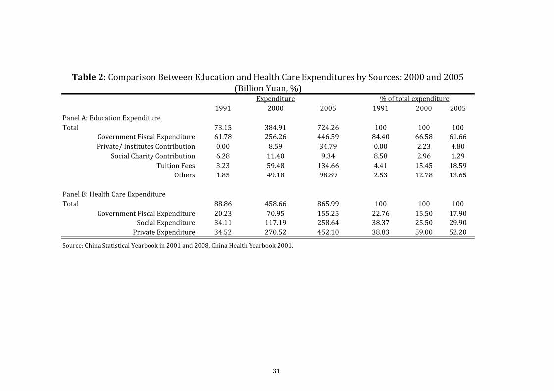
The second issue we need to discuss is the extent to which government ex-
penditure dominates the total expenditure on the provision of social services we
examine in this paper. This issue is more relevant for the education and health
services as it could be paid by private sources. The public transportation and
public security would be mainly paid for by the government. Table 2 presents
the share of government and private expenditure on education and health for
the year 1991, 2000 and 2005. The table indicates that in all three years the
government �scal expenditure accounted for more than 60% of the total expen-
diture on education, whereas only 23%, 16% and 18% of the health expenditure
in the three years, respectively, were paid for by the government. Thus, the
government contribution to health-care service provision is very limited.
2.4 Review of Related Literature
Although there is a great concern and debate over whether rural migrants impose
pressure on access to public services, city infrastructure and on increase in city
crime rates in China, few studies have provided evidence for these concerns. Yet,
there has been a large body of international immigration literature focusing on
the non-labour market impact of immigrants.
A number of studies have examined issues such as the e¤ects of immigrants
on prices (Cortes, 2008), on the housing market (Saiz, 2003), and the �scal e¤ect
(Auerbach and Oreopoulos, 1999; Storesletten, 2000). Cortes (2008) examines
the e¤ect of unskilled immigrants on the prices of non-traded goods and services
in the U.S. by using analysis based on variation across states within the U.S..
She �nds an increase in the density of unskilled immigrants in U.S. cities can
reduce prices and the channel through which the price e¤ect takes place is that
unskilled immigrant workers with low wages decrease the price of non-tradable
7

goods. A study on immigrants impact on rents and housing prices by Saiz (2003)
suggests immigrant in�ows can push up rents and housing values in destination
cities in the U.S.. Storesletten (2000) computes the net government gain of
hosting additional immigrants in the U.S. given their skill and age at the time
of immigration by using a dynamic equilibrium model of population transition.
He �nds the �scal de�cit due to an aging problem could be resolved by imple-
menting immigration policies that allow an increased in�ow of working-age high
skilled immigrants. Using the generational accounting technique, Auerbach and
Oreopoulos (1999) examine the impact of a change in immigrant in�ow in the
U.S. on the �scal burdens of current and future generations and conclude that
the impact of immigration on �scal balance is extremely small.
There is another strand of immigration literature which examines the rela-
tionship between immigration and crime (Butcher and Piehl, 1998 and 2007;
Bianchi et al., 2008). Butcher and Piehl (1998) show that when controlling
for the demographic characteristics of a city, recent immigrants appear to have
no e¤ect on crime rates and its growth rate in U.S. cities. In another study
focusing on Italy Bianchi, Buonanno and Pinotti (2008) �nd that the size of
the immigrant population is positively correlated with the incidence of property
crimes as well as with the total crime rate.
A recent study by Edlund, Li, Yi and Zhang (2007) aims at exploring the
crime rates in China and its determinants using the annual province-level data
for the period 1988-2004. Since their research interest focuses on the relationship
between male-biased sex ratios and crime rates, they only include the urbanisa-
tion rate rather than the �rate of rural-urban migrants in total city population�
as one of their control variables in the estimation regression. Their estimation
results show that urbanisation has a very modest positive e¤ect on violence
and property crime rates. However, no direct correlation between rural-urban
migration and crime rates is examined.
The above studies have di¤erent focuses. Nevertheless, the basic theory and
methodology applied in their analysis provide valuable guidance to this study.
3 Model Speci�cations and Estimation Strategy
In this study we treat cities as independent budgetary units and uses variation
across cities to examine the e¤ect of migration on the social outcomes of interest.
8

3.1 Model Speci�cation
When discussing the conceptual framework we distinguish two channels� direct
and indirect; and three e¤ects� scale, composition, and �scal, through which
rural migrant in�ow may a¤ect urban residents� access to social services or
impact on city crime rates. However, in the estimation these channels and
possible e¤ects may not be separately measured and identi�ed. The empirical
estimation, thus, will be reduced form focusing on the net impact of rural-urban
migration through all three e¤ects. The baseline model is speci�ed as below:
LnYit = �+ �Ln(R=U)it + Xit + �t + �it; (1)
where LnYit denotes the logarithm of outcome variables for city i in year t
(t = 1990; 2000 or 2005); Ln(R=U)it measures the logarithm of the ratio of
rural migrants to the total urban population for city i in year t; Xit refers to
a set of exogenous control variables which are di¤erent for di¤erent outcome
variables; and �t is the year �xed e¤ects which captures the common time e¤ect
for all cities.
The outcome variables used in Equation (1) include two education indexes,
two alternative health-care indexes, one index for public transportation, and
one measure for the city level crime rate. More speci�cally, the two proxies
for education services include teacher-student ratios for primary schools and
for junior and senior high schools. Health-care outcome is measured as the
number of hospital beds per 1000 inhabitants or the number of doctors per
1000 inhabitants. The passengers per bus is chosen as an indicator for city
public transportation. The city crime rate variable is measured as city level
prosecuted crime cases divided by the total city population. We will discuss in
details the de�nitions of these variables in the Data section.
The control variables, Xit, used for each outcome equation di¤er somewhat.
There are three common control variables for all the outcome equations: (1)
The �logarithm of real GDP per capita�is used to capture the level of economic
development in each city, which may a¤ect the level of �scal power a city has
in providing social services. (2) The �population density of the city�is used to
capture the general impact of city size. (3) The �ratio of urban-urban migrants
to total city population� is used to capture a possible competition for social
services from city-to-city migrants. It also measures the degree of population
mobility in addition to rural-to-urban migrants. Studies have found that a city
with a higher degree of regional mobility tends to have more criminal activities
9

(Rephann, 1999).8
In addition to these common control variables, the education regression also
include the �proportion of city total population aged between 6-12�for primary
school equation and the �proportion of population aged between 13-18�for ju-
nior/senior high school equation. They capture the demand side factors for
urban education. The health care regressions include the �proportion of the
total city population over the age of 65�, since more aged people may gener-
ate higher demand and put more pressure on health care facilities. For the
bus transportation regression, the �total areas within the city administrative
territory�and the �number of taxis�are chosen as control variables.
We include more control variables in the crime equation. The demographic
variable we use is �the percentage of men aged 15-40 among the total city pop-
ulation�to capture the e¤ect that young men are the demographic group most
likely to commit crime (Freeman, 1991; Levitt, 1998; Grogger, 1998). We also
follow Bianchi et al. (2008), Butcher and Piehl (1998) and Rephann (1999)
to include socioeconomic variables such as the �employment rate�and the �Gini
coe¢ cient�to proxy for economic and social conditions which may be associated
with the local crime rate.
The OLS estimation of Equation (1) on our main interest, �, may be incon-
sistent due to two potential endogeneity problems.
First, there might be a reverse causality between our outcome variables and
the migrant ratio. It can be argued that rural migrants are more likely to move
to cities where there is better public infrastructures, better social services, and
lower crime rate. or that cities with an inferior social infrastructure or high
crime rate may impose more restrictions on rural migrant in�ow. Failure to
address the reverse causality problem may lead to under-estimation of the e¤ect
of rural migrant in�ux on the outcome variables.
Second, the omitted variable problem is another potential concern. It can
be argued that some unobservable omitted variable in the error term, such as
the supply shocks due to the impact macro-economic �uctuation on city �scal
positions which may a¤ect both rural migrant in�ow and urban residents�social
outcomes.
To eliminate the endogeneity problems, we adopt �rst-di¤erence and �rst-
di¤erence with IV methods. More speci�cally, the error term �it of Equation
(1) can be decomposed into two components, i.e., �it = ui+ eit, where ui varies
8The ratio of city-to-city migrants is quite low. In the three data points we used, it is 1.1%,1.8%, and 5.0% for 1990, 2000, and 2005, respectively.
10

across cities but not over time, while eit varies across cities and over time. After
taking �rst di¤erence, the time-invariant component ui can be eliminated from
Equation (1), which can help to mitigate the endogeneity concern due to the
time-invariant city speci�c e¤ect. For example, the historical tradition of a city�s
public infrastructure, which does not vary in the short term, is correlated with
the current city infrastructure and may also be associated with the migrant
ratio. The �rst-di¤erence estimation model can be written as:
�LnYit = � + ��Ln(R=U)it + �Xit +�eit; (2)
where � indicates �rst-di¤erence, and �eit refers to the di¤erence in the time
variant part of the original error term, �it.
After taking �rst-di¤erence, there still be some unobserved factors remaining
in error term, �eit, of Equation (2), which are correlated with both the change
of log migrant ratio, �Ln(R=U)it, and the change in social outcome, �LnYit.
This endogeneity problem from the time-variant city e¤ect can be further elim-
inated by using the IV approach. In principle, the instrument used should be
uncorrelated with �eit, and strongly correlated with �Ln(R=U)it.
3.2 The Instrumental Variable9
The instrumental variable used in this study is the �rst-di¤erence in �predicted
migrant ratio�. Following the idea developed in Cortes (2008) and Boustan et
al. (2010) we use � log( bR=U)it (=[log( bRU )it � log( bRU )it�1]) as the instrument,where ( bRit) is predicted number of migrants in city i:
bRit = KXk=1
dOMkt �dPkit: (3)
The subscript k indicates the sending rural province. dOMkt is the predicted
total number of migrants from the sending rural province k at time t, and dPkitis the predicted probability of the out�ow migrants from the sending province
k to the destination city i at time t. dOMkt is obtained from the estimation of
the following equation:
OMkt = � + �Zkt�1 + �kt; (4)
9The instrument used in this paper is similar to that used in Meng and Zhang (2010).
11
where Zkt�1 is a vector of lagged push factors10 at the rural sending region,
including �land per capita�, �household income per capita�, �total land area
subject to natural disasters�, and �total machinary power for agriculture pro-
duction�.11
The probability of migrants moving from rural area k to the destination city
i (Pki) is speci�ed as a function of the quadratic in the geographic distance
between sending region k and destination city i:
Pkit = � + �kDki + �kD2ki + �kt: (5)
We estimate Equation (5) for each pair of sending region (province) k and
receiving region (city) i and the predicted probabilities (dPkit) are then obtainedfor each pair of k and i.
The di¤erence in predicted migrant ratios between time t and t�1, (log( bRU )it�log(
bRU )it�1), is then used as the instrument. The results of Equations (4) and
(5) are reported in Table A1 of Appendix A and they show that most push
factors and the distance variables are highly correlated to the migrant in�ow to
city i. We believe that none of the lagged push factors in sending regions, Zkt�1;
should have a direct e¤ect on urban local workers�social outcome variables at
receiving cities 5 to 10 years later. The variable measuring geographic distance
between k and i should also be not directly related to social service provisions
or the crime rate in city i. Thus, our instrument should satisfy the exclusion
restriction.
3.3 Estimation E¢ ciency: Seemingly Unrelated Regres-sion
It is widely believed that various urban residents social outcomes may be cor-
related with each other since all urban public services are provided by the same
local government with one budget constraint. As Zellner (1962) has pointed
out, when a common independent variable is used to explain a set of correlated
dependent variables, the correlation among these dependent variables may gen-
erate correlations among error terms across regressions through the unobserved
10We use 1985, 1990, and 2000 push variables (Zkt�1) for the 1990, 2000, and 2005 numberof out migration from sending region k, OMkt.11 In the estimation, to avoid adjustment on the size of labor force in the regression, we use
out migration rate (OMRk, de�ned as OMk divided by total rural labor force in region k) asthe dependent variable. The �nal predicted out migration (dOMk) is obtained as a product ofthe predicted out migration rate ( dOMRk) and the total rural labour force in region k.
12
cross-function constraints. Failure to consider the correlation of error terms
across regressions may overestimate standard errors for estimation coe¢ cients
and therefore could result in falsely making a conclusion of insigni�cant estima-
tion results.
In this study, the single-function estimation based on Equations (1) and (2)
as well as Equation (2) with IV estimation may su¤er from overestimation of
standard errors problem. Given the potential correlation among our outcome
variables for representing urban residents social outcome from di¤erent aspects,
there might be a signi�cant correlation among the error terms across the single-
function regressions of each social outcome index on the rural migrant ratio.
To deal with this potential problem, we use the seemingly unrelated regression
(SUR) technique (Zellner, 1962; Bartels and Fiebig, 1991) as a robustness check
to adjust standard errors for estimated coe¢ cients across all regressions based
on the OLS, �rst-di¤erence, and �rst-di¤erence with IV estimations.12
4 Data and Summary Statistics
4.1 Data
The data used for this paper are mainly taken from two sources. The �rst data
source is the China Population Censuses and Population Survey including the
1 percent micro-data sample of the 1990 and 2000 Censuses and the 20 percent
micro-data sample of the 2005 1 percent Population Survey. These Censuses
and/or Population Survey are conducted by the National Bureau of Statistics
of China (NBS). They provide individual demographic information consistent
across years. The advantage of these data for this study is that they cover
everyone who lived in the city at the time of the survey for more than six months
including rural migrants. Thus they can be used to measure, more accurately
than normal survey data, the relative size of rural migrants with respect to the
urban population in each Chinese city. Therefore, the main explanatory variable
used here� the share of rural migrants to urban population for each city (i.e.,
migrant ratio)� is calculated from this data source.
The second data source is the 1992,13 2001, and 2006 City Statistical Year-
12SUR is better applied based on the large-sample properties of �large T , small N�data setsin which T ! 1 (Baum, 2006). Since our data have a relatively large N (number of cities)and small T (three data points), SUR is only used as a robustness check.13As the censuses were conducted in 1990 and 2000 and the population survey was in 2005,
ideally we would like to use the dependent variables also in those years. However, the data
13

books of China. The data from this source are collected by the NBS on an
annual basis. The data set provides a wide range of detailed city-level infor-
mation including macro-economic and social service outcomes in the previous
calendar year (i.e., the years of 1991, 2000 and 2005). Most part of these data is
available to the general public, but the use of the crime rate data requires special
permission. The dependent variables - urban residents social service outcome
variables and crime rates - are mainly constructed from these data.
The combination of the two data sources generates an unbalanced city panel
data over the three data points in 1990, 2000 and 2005. The number of cities
at the county or above level in China has been increasing over time. Excluding
missing values, our �nal data consist a balanced panel of 152-city over three
data points.
4.2 De�nition of Dependent Variables
The dependent variables used in this paper are proxies for four types of social
service access, namely education, health, public transport, and public security.
We use two variables, the teacher-student ratios for primary school and
for junior/senior high schools in the city, to capture education access at these
two levels. The numerators are the number of teachers at each level, while
the denominators are the number of enrolled students at each level including
enrolled migrant children. Ideally we would like to include only junior high
school teacher-student ratio for the second measure, as only primary and junior
high school are the level of education at which migrant children are more likely
to have access to, and hence, have possible crowding out e¤ect on the access
of local residents. However, the data on number of teachers for the secondary
school is combined of junior and senior high school.
Two alternative health service measures, the number of hospital beds and
the number of doctors per 1000 inhabitants, are used to address the issue of
health care access from di¤erent perspectives. The variables are de�ned as the
total number of beds in hospitals and clinics and the total number of doctors
divided by the total population, including migrant population. Ideally we would
wish to have number of hospital beds or doctors per 1,000 patiants as that
will be an accurate measure of health services provided, but such data are not
available to us.
collection system for the City Statistical Yearbook data changed between 1991 and 1992 for theyear 1990 and 1991. Thus, to keep the de�nition of our major dependent variables consistent,we use 1992 City Statistical Yearbook data for the year 1991 rather than 1990.
14

The public transportation access is proxied by the total number of passengers
per bus. It is de�ned as the total volume of bus/tram passengers for the whole
year divided by the number of buses/trams at the end of year. Note that since
there is no information on the frequency of bus/tram usage, we assume the
frequency does not change over time and across cities.
In terms of crime rate, the only variable available in the data is the number
of prosecuted crime cases. We use this variable divided by total city population
(including migrant population) to obtain the city crime rate. Of course, the
number of prosecuted crime cases is not a perfect proxy for the actual crime
rate since it might be in�uenced by the legislative enforcement of a city. If,
for example, a city�s legislative authority has a strong concern about rural-
urban migration and hence prosecute more migrant crime cases, then number
of prosecuted crime cases might be positively correlated with rural migrant
density of the city. Thus, using such an index as the dependent variable may
lead to an overestimation of the �net�e¤ect of migrant in�ow on the city crime
rate.
4.3 Summary Statistics
Table 3 presents the summary statistics for all the outcome variables and the
major independent variables14 based on the 152 city sample. The table shows
that in 1991 the teacher-student ratio for primary schools in Chinese cities was
5.2 teachers per 100 students. This number increased slightly over the next
15 years to 5.4 in 2000 and 5.7 in 2005. The resource in secondary school are
better with 100 students sharing 6.5 teachers in 2005. These ratios are quite
high on developing country standards. The teacher-student ratio for primary
school children in India in 2001, for example, was only 2.5 per 100 students.
Over the 15 years, the accessability of the medical services seem to have de-
teriorated in Chinese cities. In 1991 the number of hospital beds and number of
doctors per 1000 population was 6 and 4, respectively, but by 2005 the numbers
reduced to 5.7 and 2.9. This phenomenon may be partially related to the decen-
tralization of the health-care expenditure. Table 2 shows that the government
�scal expenditure contributed to 23% of the total health expenditure in 1991,
but 18% in 2005, whereas private expenditure contributed to 39% in 1991 and
52% in 2005. It could also be related to the fast urbanization process.
The situation of transportation over time has improved. The number of
14Appendix Table 2 presents the sources and de�nitions of the major independent variables
15

passengers per bus/tram reduced from 279 in 1991 to 140 in 2000, and then
increased slightly to 150.
The most signi�cant change among the outcome variables is probably the
number of criminal cases prosecuted per thousand population. It increased
from 3.4 in 1991 to 7 in 2005. Once again, this may be related to the rapid
urbanization over this period.
Regarding the urbanization process, the average of the total city population
has increased from 1.1 million in 1991 to 1.7 million in 2005.15 The average
proportion of rural migrants in total population increased from 7% to 12%, and
the proportion of urban-urban migrants increased from 1 to 5%. At the same
time while the urban population is increasing, urban areas are enlarging. Thus,
over time the average city population density is reducing slightly from 1500 per
square-kilometers to 1300 per square-kilometers.
To understand the relationship between the main outcome variables and the
city migration ratio, we plot the unconditional correlations in Figures 2 and 3.
Figure 2 presents the correlation for each year, while Figure 3 illustrates the
relationship between the �rst-di¤erences of each of the outcome variables and
that of the migrant ratio.
When examining the level di¤erences, we �nd that the variation of migrant
ratios across di¤erent cities seems to be correlated to both the teacher/student
ratio at primary level and the crime rate. No other strong correlation is found.
However, when we take the �rst-di¤erences the results changed. The change
in migrant ratio does not seem to have any relationship with the change in
teacher-student ratio at the primary school level, but a positive e¤ect on the
change at the junior high school level. For health services there seems to be
a slight reduction in number of hospital beds and number of doctors for cities
where migrant ratio increases. The e¤ect of change in migrant ratio seem to be
associated with a increase in passengers per bus between 1991 and 2000, but a
reduction between 2000 and 2005. The relationship between migrant ratio and
the crime rate exhibit the most signi�cant di¤erence between Figures 2 and 3.
When looking at the �rst-di¤erences, we �nd no correlation between the change
in migrant ratio and crime rate in the �rst period (1991-2000) and a negative
correlation in the second period (2000-2005).
These graphs provide some indications as to how the variations in the out-
15There are two measures of total urban population, one from the City Statistical Yearbooksand the other from the Population Censuses and Population Survey Data. Both two measuresare reported in Table 3 and they are quite close.
16
come variables across cities are associated with migrant distributions across
cities and over time. Their conditional relationship will be examined in details
next.
5 Estimation Results
Equations (1) and (2) are estimated for each of the outcome variables of access
to social services and the crime rate.
5.1 HowRural-UrbanMigration A¤ects Urban Residents�Social Service Accession
How do rural migrants a¤ect urban residents�access to social services in China?
We examine the impact on education, health care, and transport accesses sep-
arately.
5.1.1 Education
Table 4 reports the results of the impact of migration on teacher to student ratios
at the primary school (Panel A) and secondary (junior and senior) schools (Panel
B). The dependent variable is the total number of teachers per 100 students in
respective levels of schools.
The �rst column of Panel A reports the OLS results for the primary school
teacher-student ratio. The estimated coe¢ cient for the log migrant ratio is
negative (-0.073) and statistically signi�cant at the 1 percent level, suggesting
an increase in migrant ratio of 1 per cent is associated with a reduction in the
teacher to student ratio of 0.07 percent. Controlling for the urban population
demand e¤ect (city population density and the proportion of 6 to 12 years old
of primary school age), the negative correlation between the teacher to student
ratio and migrant ratio seems to suggest that cities (and across time) where
there are more migrant population there are less investment in primary school
education.
However, the correlation observed in the OLS regress may not imply a causal
relationship. To examine the causal impact, we estimate the �rst-di¤erence and
�rst-di¤erence with IV models. When taking �rst-di¤erence to control for time-
invariant city speci�c e¤ect (see Column (2)), the e¤ect of the migrant ratio
on the teacher-student ratio reduced dramatically and becomes statistically in-
17

signi�cant. Such a change implies the negative and signi�cant e¤ect obtained
from the OLS estimation may be caused by variations across cities which af-
fect both the migrant ratio and teacher to student ratio. For example, if cities
which invested more on primary education at a given demand also restricted
migrant in�ow, a negative relationship might be observed between the migrant
ratio and teacher to student ratio in an OLS estimation. If this is the case,
the �rst-di¤erence estimation may reveal the real e¤ect of the migrant ratio on
the teacher to student ratio by controlling for this unobserved variation across
cities. In this sense the �rst-di¤erence estimation is better than OLS but it still
cannot eliminate the time-varying within-city unobservable e¤ect in error terms.
First-di¤erence with IV estimation can further eliminate this type of potential
endogeneity. Column (3) of Table 4 shows that when controlling for all sources
of potential endogeneity problem and controlling for other observable city level
characteristics, rural migrant in�ow has a slight positive but statistically in-
signi�cant e¤ect on the primary school teacher to student ratio.
The level of economic development, measured by log per capita GDP is posi-
tively associated with teacher/student ratio. However, the relationship between
the change in teacher-student ratio and economic growth (the �rst di¤erence
measure of log per capita GDP) is not precisely estimated. In addition, urban-
urban migration is positively associated with teacher-student ratio, population
density is negatively associated with teacher-student ratio, whereas other con-
trol variables are not statistically signi�cant.
Panel B of Table 4 (Columns 4-6) reports the same set of results for the
middle school (both junior and senior high schools combined) teacher-student
ratio. In this estimation, the density of total city population and the proportion
of 13-18 years old (middle school age) in the city population are used to control
for the demand side of the e¤ect.
Di¤erent to the results for the primary school, the OLS estimate of the
correlation between the migrant ratio and middle school teacher-student ratio
is not statistically signi�cant, but the �rst-di¤erence and �rst-di¤erence with IV
estimations both reveal positive and statistically signi�cant e¤ects of migration
on the teacher-student ratio. In particular, the �rst-di¤erence with IV result
indicates that every one percent increase in migrant ratio induces 0.07 percent
increase in teacher-student ratio at secondary school level. This result indicates
that perhaps the indirect ��scal e¤ect�dominates the direct �scale e¤ect�. That
is to say that migrants as taxpayers contribute signi�cantly to cities�investment
in secondary education, whereas as consumers their consumption of secondary
18

education is limited. This is quite intuitive given that even today migrant
children are not eligible to attend public senior high schools in cities.
In summary, the above �ndings suggest rural migrant in�ow does not impose
a negative impact on urban primary and middle school education. If anything,
migrant in�ow contributes slightly positively to the teacher to student ratios at
secondary school level. These results are not surprising. As discussed before,
migrant parents do not normally bring their children to cities. When they do
they often send their children to migrant-funded non-public schools even though
the quality of these schools are very low.
5.1.2 Health
The second relationship investigated is the impact of rural migrant in�ow on
urban residents� access to health-care services. The results are presented in
Table 5.
Panel A of Table 5 presents the results on the number of hospital beds
per 1000 people. The coe¢ cient for the migrant ratio based on the OLS has
a negative and statistically signi�cant e¤ect. An 1 percent increase in migrant
ratio reduces hospital beds per 1000 people by 0.056 percent. However, when we
take �rst-di¤erence the e¤ect completely disappears. The �rst-di¤erence with
IV (Column [3]) also produces a near zero e¤ect (0.005). This indicates that
rural migrant in�ow have no impact on health service provisions measured by
number of hospital beds per 1,000 population. The general demand factors, such
as the ratio of the ageing population and population density are all positively
related to hospital beds per 1000 population. The GDP level and its growth, the
supply factor, are also signi�cantly positively related to hospital beds provisions.
The results obtained from using the number of doctors per 1000 inhabitants
as a proxy for health service provision are di¤erent. In all three cases (OLS,
�rst-di¤erence, and �rst-di¤erence with IV) the results suggest negative impact
of migrant in�ow on number of doctors per 1000 people (Panel B of Table 5).
The coe¢ cient from the �rst-di¤erence with IV indicates that an additional 1
percent increase in migrant in�ow reduces number of doctors per 1000 people
by 0.08 percent, which is a very small impact.
Note that the dependent variables we use here are number of hospital beds or
doctors per 1,000 people (potential users) not per 1,000 patients (actual users).
Thus, no matter migrants use the services or not, cities with more migrants
will have lower measure of health services keeping the numerators (number of
19

hospital beds or doctors) and number of urban residents constant. Therefore,
our estimated results in fact only measure the supply side of the e¤ect. That is
whether cities with more migrants invest more on health services or not.
There are many reasons for us to believe that relative to urban local residents,
migrants are less likely to use the health services. One reason is that migrants
on average are primary aged adults, hence, relatively healthier than the average
urban local population. Another reason is that most migrants are not covered
by health insurance in cities. When they are sick they try to avoid to go to
hospitals or to see doctors. The RUMiCI 2009 survey shows that of the 1374
migrants who reported to be sick in the past three months prior to the survey
date, 47 percent saw a doctor or went to the hospital while the remainders
simply bought medication from the pharmacies, had a rest, or did not take any
action. In comparison, of the 2374 urban hukou residents who were sick in the
three months leading to the survey date, 77 percent went to see a doctor or to a
hospital. When migrants are seriously ill, they normally go back to their rural
home towns where they have some sort of health insurance but the quality of
health care are much worse than in cities.
Given that migrants as taxpayers contribute to city revenues but less likely
to consume health services than their local counterparts, it is reasonable for
cities with more migrants to invest less on health care services. This, however,
does not imply a reduced services to actual health-care service users. The small
adverse e¤ect we observed in this paper may simply re�ect the artifact that
cities with more migrants have more potential users but less actual users.
Another important issue to bear in mind when interpreting the results on
health care services is the fact that the health care in China during the period
we study was predominantly funded by a user-pay system and the government
contribution to health-care provision is very limited as shown in Table 2. Thus,
the migrant in�ow causes cities to have less health-care users, hence lower fund-
ing for health-care, but their contribution to health care provision made through
them being taxpayers maybe somewhat limited. Thus, the small negative causal
e¤ect we observed for number of doctors per 1000 people should have very lim-
ited implications on the actual access of health-care services the urban residents
receive.
20

5.1.3 Public transportation
The total number of passengers per bus is chosen as the index of the intra-city
public transportation access. In order to control for demand side factors, the
urban population density, the city geographic area, and the number of alterna-
tive transportation vehicles (i.e., taxis) are included as control variables in the
estimation. The results are reported in Table 6.
The OLS coe¢ cient for the migrant ratio is positive with a coe¢ cient of
0.10 and signi�cant at the 5 percent level. This suggests a higher migrant ratio
is associated with a larger number of passengers per bus. The �rst-di¤erence
reduces the result somewhat but still highly signi�cant. Controlling for both
time variant and time invariant unobservable characteristics which may a¤ect
both migration and urban transportation (Column [3]) results in a positive
e¤ect. The magnitude of the coe¢ cient is much larger (0.17) than that obtained
in the OLS regression but the point estimate is not precise. The result seems to
indicate that the increase in migrant in�ow increases pressure on cities�public
transportation service.
The results we obtained so far seem to suggest that migrants in�ow put
certain pressure on cities transportation service, but have no adverse e¤ect on
education or health services.
5.2 How Rural-Urban Migration A¤ects City Crime Rate
It has been a common belief that migrant in�ow increases city crime rates. If
we simply examine the unconditional correlation, the data seem to support this
view. Figure 1 shows that there is a strong positive relationship between the log
number of prosecuted criminal cases per thousand persons and the log migrant
ratio. However, this unconditional correlation may be an illusion. It is known
that a large proportion of the migrant population is males aged 15 to 40, and this
group is more prone to committing crime (Freeman, 1991; Levitt, 1998; Grogger,
1998). Migrants are more likely to move into cities with higher population
density and industrialisation level, where higher crime rates are often found
in the literature (Rephann, 1999). Thus, the simple unconditional correlation
may be misleading. Furthermore, once we take �rst-di¤erence, the clear positive
relationship disappeared. The �rst-di¤erence unconditional relationship is slight
positive between 1990-2000, but negative between 2000 and 2005 (Figure 3).
To understand the true e¤ect of rural-urban migration on city crime rates,
we estimate Equations (1) and (2). In addition to the common control vari-
21

ables as in all the other estimations, we also control for the fraction of male
population between 15-40 in the total city population, the ratio of urban-urban
migration, the employment rate of the urban labour force, and the city level Gini
coe¢ cients.16 These variables are widely believed to be related to city crime
rates (Butcher and Piehl, 1998; Bianchi et al., 2008). The estimated results are
reported in Table 7.
We �rst estimate a simple correlation between the log crime rates and log
migrant ratio, controlling only the year e¤ect (Column [1] of Panel A). As
expected, the result is positive and signi�cant. The magnitude indicates that
every one percent increase in migrant ratio increases the city crime rates by 0.27
percent. In order to test this positive e¤ect is related to the fact that rural-urban
migrants are more likely to be young men who are more prone to committing
crime we add in a variable indicating �the proportion of males (including both
local and migrants) aged 15-40 to that of total urban population�. Such an
inclusion reduces the estimated elasticity substantially to 0.19 but it is still
statistically signi�cant at the 1 percent level (Column [2]). As expected, the
variable �proportion of male aged 15-40�is positively associated with crime rate
and the estimated elasticity is huge, 1.51, almost eight times of that observed
for migrant ratio.
We then include the other control variables and the estimated elasticity on
log migrant ratio further reduced to 0.13 and the signi�cant level reduced to the
10 percent (Column [3]). Other control variables we include all have the right
signs. It is commonly found that GDP per capita has a positive relationship
with the crime rate, and employment rate is negatively associated with the
crime rate. Further, if migrants are more likely to be young males, urban-to-
urban migration should also have a positive correlation with crime rate. We
also �nd that the crime rate in 2005 is statistically signi�cantly higher than
previous years. These �ndings seem to suggest that the crime incidence in cities
is strongly associated with its demographic features of total population as well
as economic conditions.16Gini coe¢ cients are calculated using Urban Household Survey (UHS) data for the year
1990, 2000, and 2005. There are two issues related to using Gini coe¢ cients. First, the UHSsurvey only covers 63 of the 157 cities we use in this paper. To make sure our results areconsistent, we estimate the crime equation using two di¤erent speci�cations, one with full 157city sample but without Gini coe¢ cient as control variables, and one with Gini coe¢ cient butfor a subset of the sample. The latter results are reported in Panel B of Table 5. The secondissue is related to the fact that UHS only include urban local workers and migrants are notincluded. This may under-estimate the degree of inequality. We test the sensitivity of thisproblem by comparing Gini coe¢ cients calculate from the 2005 1% population survey data,which include migrants, and those obtained from using the 2006 UHS data.
22

Although the OLS estimation reveals a small and statistically signi�cant
relationship between the migration ratio and city crime rate, this result su¤ers
from the endogeneity problem as discussed before. The estimates with �rst-
di¤erence and �rst-di¤erence with IV, which mitigate the endogeneity problem,
are presented in columns [4] and [5] of Table 7. The relationship between the
change in city crime rates and the change in migration ratios controlling for the
other independent variables is slightly negative, but not signi�cant. Whereas the
�rst-di¤erence with IV results a very small positive and statistically insigni�cant
e¤ect.
The above results did not control for the Gini coe¢ cients, which is commonly
believed to have some correlation with crime rates, because we only have a
sub-sample of cities with the Gini coe¢ cient measure. Panel B presents the
results including Gini coe¢ cients as an additional independent variable for this
subsample of cities, while Panel C exhibits the results without Gini coe¢ cient
control for the same group of cities. Comparing the results from Panels B and
C we �nd that controlling for the Gini coe¢ cients does not a¤ect our main
�nding that the variation in the migrant ratio across cities has no impact on
the variation of the crime rates across cities.
The result that migrant in�ow has no impact on city crime rates is quite
di¤erent from the common belief that migrants are more prone to committing
crime. But thinking carefully it is quite understandable. Due to the restrictions
on migrant access to social services in cities, they only come to cities to work
so that they can bring home as much money as possible. As a result, migrant
workers on average work 7 days a week and more than 10 hours daily (Du et al.,
2006; Lee and Meng, 2009). Given their working schedule it is almost impossible
for them to spend too much time committing crimes.
A potential drawback of our crime rate measure must be born in mind.
As the only crime data available for the analysis is the number of prosecuted
criminal cases rather than the crime cases committed, it is possible that migrants
could have in fact committed much more crime but that not all of them were
apprehended. For example, if some migrants commit crime just prior to leaving
for their home villages they are unlikely to be caught. If this is the case, the
measure of the crime rate used in this paper may not re�ect the actual crime
rate for a city or the actual e¤ect of migration in�ow on the city crime rate.
Nevertheless, this would only have an impact on our results if the measurement
error in crime rate vary signi�cantly across cities. We have no reason to believe
that this is the case.
23

5.3 Robustness Check
In this subsection we conduct the following robustness checks.
First, the analysis presented above on the e¤ects of migration in�ow on
urban residents� access to various types of social services and on city crime
rates treats each of the outcome variables as independent. However, all these
outcome variables may in fact be related through government spending. To test
sensitivity we use the Seemingly Unrelated Regression (SUR) to estimate all
social service outcomes and the city crime rate regressions jointly, so that the
error terms across di¤erent equations are correlated. The results using �rst-
di¤erence with IV method are reported in Table 8.
We �rst treat hospital beds and doctors as alternative health care measures
and estimate the �ve equations (excluding one of the health care measures)
jointly (Columns [2] and [3]) and then we treat them both as part of the decisions
the governments make when decide where to spend the money (Column [4]).
Finally, as spending on public security only indirectly a¤ect crime rate, we also
estimate �ve equations excluding the crime rate equation (Column [5]). The
results from the SUR estimation, that allows error terms to be correlated across
the equations, are largely consistent with those observed from the single equation
estimation (Column [1] of Table 8 reproduces these single equation estimation
results), but the estimation precision are slightly improved. The major change
is that the estimated elasticity of migrant ratio on �number of hospital beds
per 1,000 population� is now negative, but still statistically insigni�cant when
crime rate is included in the equation. When we exclude crime rate from the
SUR estimation, though, this elasticity becomes signi�cant at the 10 percent
level with a small magnitude (-0.06).
Second, as shown in Figure 3 that the relationship between the �rst-di¤erence
in migrant ratio and in the hospital beds per 1,000 population, the number
of doctors per 1,000 population, the passengers per bus, and the crime rate
all di¤er somewhat across years. We would like to know whether the causal
impact of migration rates on these outcome variables also vary across years. We
interact the migrant ratio variable with the year dummy variable and interact
the instrument with the year dummy variable as well to generate an additional
instrument. Table 9 presents the �rst-di¤erence and �rst-di¤erence with IV
results on these outcome variables.
The �rst-di¤erence results indicate that the main adverse impact of increase
in migrant in�ow on reduction in �doctors per 1,000 persons�and increase in
24

�passengers per bus�occurred between 1990 and 2000. The change in migrant
ratio between 2000 and 2005 has no impact on doctor supply and it reduced
�passengers per bus�. For the crime rate equation we observe a statistically
signi�cant impact of increase in migrant ratio on reduction in crime rate in the
second period, which is consistent with the unconditional relationship observed
in Figure 3.
When using �rst-di¤erence with IV method, the estimated coe¢ cients for
both the �doctors per 1,000 persons� and �passengers per bus� equations are
more than doubled in size and that for the �crime rate� equation, both coef-
�cients switched sign. We take this as an indication of the weak IV. Indeed,
the F-tests for the IV used for the interaction term are all less than 10. We
therefore decide not to interpret these results.
Finally, as discussed in footnote 16 the Gini coe¢ cients used in Table 7 are
calculated using UHS data, which do not include migrant population. This may
under-estimate the actual inequality within each city. To the extent that the
level of under-estimation does not systematically di¤er cross cities our results
should not be biased. Fortunately the 2005 1% Population Survey data have
information on individual income, which enable us to calculate city level Gini
coe¢ cients for all city population including migrants. For this year, therefore,
we can test whether the cross-city variation in Gini coe¢ cients di¤ers between
those calculated using data without migrants (UHS) and with migrants (Popu-
lation Survey data). Figure 4 presents the unconditional relationships between
crime rates and Gini coe¢ cients measured using UHS and Population Survey
Data. The relationship are very similar.
6 Conclusions
Based on the increasing concern of the urban public about rural-urban migration
and its social impact, this paper investigated the link between rural migrant
in�ows and various social outcomes, including the level of urban locals�access
to social services and the city crime rate.
In terms of urban social services, we found that rural migrant in�ow imposed
no adverse e¤ect on education. If anything, we found it to increase secondary
school resources as re�ected in the number of teachers per 100 enrolled stu-
dents. This perhaps is due mainly to the fact that migrants contribute to the
tax revenue but consume very little of secondary education resources. Some
25
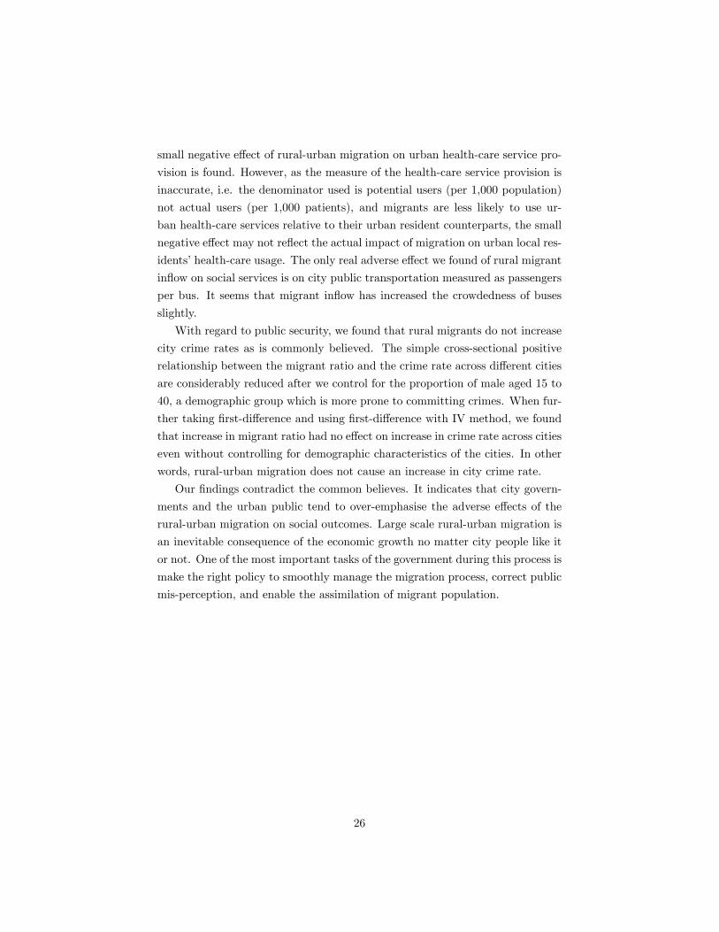
small negative e¤ect of rural-urban migration on urban health-care service pro-
vision is found. However, as the measure of the health-care service provision is
inaccurate, i.e. the denominator used is potential users (per 1,000 population)
not actual users (per 1,000 patients), and migrants are less likely to use ur-
ban health-care services relative to their urban resident counterparts, the small
negative e¤ect may not re�ect the actual impact of migration on urban local res-
idents�health-care usage. The only real adverse e¤ect we found of rural migrant
in�ow on social services is on city public transportation measured as passengers
per bus. It seems that migrant in�ow has increased the crowdedness of buses
slightly.
With regard to public security, we found that rural migrants do not increase
city crime rates as is commonly believed. The simple cross-sectional positive
relationship between the migrant ratio and the crime rate across di¤erent cities
are considerably reduced after we control for the proportion of male aged 15 to
40, a demographic group which is more prone to committing crimes. When fur-
ther taking �rst-di¤erence and using �rst-di¤erence with IV method, we found
that increase in migrant ratio had no e¤ect on increase in crime rate across cities
even without controlling for demographic characteristics of the cities. In other
words, rural-urban migration does not cause an increase in city crime rate.
Our �ndings contradict the common believes. It indicates that city govern-
ments and the urban public tend to over-emphasise the adverse e¤ects of the
rural-urban migration on social outcomes. Large scale rural-urban migration is
an inevitable consequence of the economic growth no matter city people like it
or not. One of the most important tasks of the government during this process is
make the right policy to smoothly manage the migration process, correct public
mis-perception, and enable the assimilation of migrant population.
26
References
[1] Altonji, Joseph and David Card, �The e¤ects of immigration on the labor
market outcomes of less-skilled natives�, in J. M. Abowd and R.B. Free-
man eds., Immigration, Trade, and the Labor Market, Chicago: Chicago
University Press, 1991 Sep.
[2] Auerbach, Alan J. and Philip Oreopoulos, �Analyzing the Fiscal Impact of
U.S. Immigration�, The American Economic Review, 89(2), 176-180, 1999
May
[3] Bartels, Robert and Denzil G. Fiebig, �A Simple Characterization of Seem-
ingly Unrelated Regressions Models in Which OLS Is BLUE�, The Amer-
ican Statistician, 45(2), 137-140, 1991 May.
[4] Becker, Gary S., �Crime and Punishment: An Economic Approach�, The
Journal of Political Economy, 76(2), 169-217, 1974.
[5] Bianchi, Milo, Paolo Buonanno and Paolo Pinotti, �Immigration and
Crime: An Empirical Analysis�, BANCA D�ITALIA (The Central Bank
of Italy) Working Papers No. 698, 2008 Dec.
[6] Butcher, Kristin F. and Anne Morrison Piehl, �Recent Immigrants: Un-
expected Implications for Crime and Incarceration�, Industrial and Labor
Relations Review, 51(4), 654-679, 1998.
[7] Butcher, Kristin F. and Anne Morrison Piehl, �Why Are Immigrants�In-
carceration Rates So Low? Evidence On Selective Immigration, Deterrence,
and Deportation�, National Bureau of Economic Research Working Paper
No.13229, 2007 Jul.
[8] Boustan, Leah Platt, Price V. Fishback and Shawn E. Kantor, �The E¤ect
of Internal Migration on Local Labor Markets: American Cities During the
Great Depression�, Journal of Labor Economics, 28(4), pp.719-746, 2010.
[9] Cortes, Patricia, �The E¤ect of Low-Skilled Immigration on U.S. Prices:
Evidence from CPI Data�, The Journal of Political Economy, 116(3), 381-
422, 2008, Jun.
[10] Du, Yang, Robert Gregory and Xin Meng , �Impact of the Guest Worker
System on Poverty and Wellbeing of Migrant Workers in Urban China�,
27

in Ross Gaunaut and Ligang Song eds., The Turning Point in China�s
Economic Development, Canberra: Asia Paci�c Press, 2006 Mar.
[11] Edlund, Lena, Hongbin Li, Junjian Yi and Junsen Zhang, �Sex Ratios and
Crime: Evidence from China�s One-Child Policy�, IZA Discussion Paper,
Insitute for the Study of Labor, the University of Bonn, Bonn, Germany,
2007 Dec.
[12] Ehrlich, Isaac, �Participation in Illegitimate Activities: A Theoretical and
Empirical Investigation�, The Journal of Political Economy, 81(3), 521-565,
1973 May-Jun.
[13] Feng, Shuaizhang and Yuanyuan Chen, �School type and education of mi-
grant children: Evidence from Shanghai (in Chinese)�, Economics Quar-
terly, forthcoming.
[14] Freeman, R. B., �Crime and the Employment of Disadvantaged Youths�,
National Bureau of Economic Research Working Paper No. 3875, 1991.
[15] Frijters, Paul, Robert Gregory, and Xin Meng, �The role of rural migrants
in the Chinese urban economy �, Working Paper, University of Queensland
,2011.
[16] Glaeser, Edward L. and Bruce Sacerdote, �Why Is There More Crime in
Cities�, The Journal of Political Economy, 107(6), S225-S258, 1999 Dec.
[17] Gong, Xiaodong, Sherry Tao Kong, Shi Li and Xin Meng, �Rural-urban
migrants, A driving force for growth�, in L. Song, R. Garnaut and W. T.
Woo eds., China�s Dilemma, Economic Growth, the Environment and Cli-
mate Change, Brookings Institution Press/ANU e-Press with Asia-Paci�c
Press, 110-151, 2008 Oct.
[18] Grogger, J., �Market Wages and Youth Crime�, Journal of Labor Eco-
nomics, 16(4), 756-791, 1998.
[19] Leng, Lee, and Xin Meng, �Why don�t more Chinese migrate from the
countryside? Institutional constraints and the migration decision�, in X.
Meng, C. Manning, S. Li, and T. E¤endi eds., The Great Migration: Rural-
Urban Migration in China and Indonesia, Edward Elgar Publishing Ltd.,
2009.
28

[20] Levitt, S. D., �Juvenile Crime and Punishment�, The Journal of Political
Economy, 106(6), 1156-1185, 1998.
[21] Liu, Chengfang, �Educating Beijing�s Migrant Children: A Pro-
�le of the Weakest Link in China�s Education System�, http://iis-
db.stanford.edu/docs/274/CFLIU_educating_Beijing_migrants_FF_Apr2010.pdf,
2010.
[22] Meng, Xin and Junsen Zhang, �The Two Tier Labor Market in Urban
China: Occupational and Wage Di¤erentials Between Residents and Rural
Migrants in Shanghai�, Journal of Comparative Economics, 29(3), 485-504,
2001.
[23] National Bureau of Statistics of China (NBS), �Number of Rural Workers
in Chinese Cities Was 225.42 Million By the End of 2008 (in Chinese)�,
http://www.stats.gov.cn/tjfx/fxbg/t20090325-402547406.htm , 2009 Mar.
[24] Rephann, Terance J., �Links Between Rural Development and Crime�,
Papers in Regional Science, 78, 365-386, 1999.
[25] Research Team of the State Council, Research Report on Rural-Urban Mi-
gration in China (in Chinese), Beijing: China Yanshi Press, 2006 Apr.
[26] Saiz, Albert, �Immigration and Housing Rents in American Cities�, Journal
of Urban Economics, 61(2), 345-371, 2007 Mar.
[27] Sheng, Laiyun and Liquan Peng, �The Population, Structure and Charac-
teristics of Rural Migrant Workers (in Chinese)�, Research on Rural Mi-
grant Labour in China, Beijing: China Statistics Press, 2005
[28] Storesletten, Kjetil, �Sustaining Fiscal Policy through Immigration�, The
Journal of Political Economy, 108(2), 300-323, 2000.
[29] Xu, Guangjian, Zhaoyu Gao, and Yu Zhao, �Review and expectation on
Chinese �scal reform since 1978 (in Chinese)�, Journal of Shanxi Finance
and Economics University, 31(2), 19-27, 2009.
[30] Zellner, A., �An E¢ cient Method of Estimating Seemingly Unrelated Re-
gressions and Tests for Aggregation Bias�, Journal of American Statistical
Association, 57, 348-368, 1962.
29

Total government fiscal expenditure Central Gov. Local Gov.
% of local fiscal expenditure
[1] [2] [3] [3]/[1]Total Expenditure 3393.03 878.79 2514.23 74.10%
Education 397.48 24.49 373.00 93.84% Health 103.68 2.13 101.56 97.95%
Source: China Statistical Yearbook in 2006.
Table 1: Central and Local Government Fiscal Expenditure among Education, Health Care and City Service (2005) (Unit: billion Yuan, %)
30
1991 2000 2005 1991 2000 2005Panel A: Education ExpenditureTotal 73.15 384.91 724.26 100 100 100
Government Fiscal Expenditure 61.78 256.26 446.59 84.40 66.58 61.66Private/ Institutes Contribution 0.00 8.59 34.79 0.00 2.23 4.80
Social Charity Contribution 6.28 11.40 9.34 8.58 2.96 1.29Tuition Fees 3.23 59.48 134.66 4.41 15.45 18.59
Others 1.85 49.18 98.89 2.53 12.78 13.65
Panel B: Health Care ExpenditureTotal 88.86 458.66 865.99 100 100 100
Government Fiscal Expenditure 20.23 70.95 155.25 22.76 15.50 17.90Social Expenditure 34.11 117.19 258.64 38.37 25.50 29.90
Private Expenditure 34.52 270.52 452.10 38.83 59.00 52.20
Source: China Statistical Yearbook in 2001 and 2008, China Health Yearbook 2001.
Expenditure % of total expenditure
Table 2: Comparison Between Education and Health Care Expenditures by Sources: 2000 and 2005 (Billion Yuan, %)
31

1990/1991 2000 2005Number of teacher per 100 student in primary school 5.18 5.44 5.71
(0.97) (1.24) (1.16)Number of teacher per 100 student in junior/senior middle school 7.68 6.27 6.47
(1.21) (1.15) (1.15)Number of hospital bed per 1000 inhabitants 6.09 5.79 5.74
(1.95) (1.84) (1.77)Number of doctor per 1000 inhabitants 4.05 3.12 2.92
(1.45) (1.13) (0.97)Volume of passengers per bus for the whole year (10 thousand times) 278.59 142.60 151.05
(165.19) (76.63) (63.74)Number of criminal cases 3512.88 8729.87 12675.28
(5021.50) (16890.28) (18424.51)Number of criminal cases per thousand inhabitants 3.39 5.62 6.99
(3.27) (5.69) (5.31)Total number of population at the end of survey year (thousand people) 1082.60 1433.47 1715.64
(1119.98) (1744.07) (2073.23)Total number of city population (thousand people)a 1266.33 1486.49 1777.20
(1345.32) (1919.76) (2040.31)Proportion of rural migrants among total city population (%) a 7.03 8.18 11.62
(5.81) (8.46) (11.52)Real GDP per capita (Yuan/Person) 5156.83 18188.19 32499.83
(3602.99) (15468.83) (18260.84)City population density (thousand people per Km2) 1.50 1.40 1.30
(1.29) (1.01) (0.95)Urban-urban migrant ratio (%) a 1.09 2.82 4.99
(2.06) (1.96) (3.53)Proportion of population aged between 6-12 (%) a 4.93 4.88 4.94
(2.29) (1.54) (1.53)Proportion of population aged between 13-18 (%) a 4.71 5.76 5.40
(2.99) (1.59) (1.63)Proportion of aged population (>=65) (%) a 3.11 4.10 5.66
(1.81) (1.62) (4.67)Total land areas of adminstrative region (Km2) 1285.30 1750.09 2067.09
(1962.40) (2603.59) (2989.23)Number of taxis 1120.90 4183.32 4319.38
(3055.10) (7333.19) (7482.88)Proportion of males aged 15-40 among total city population (%) a 26.10 23.91 21.71
(4.03) (2.23) (2.75)
Employment rate (%) a 95.92 86.98 89.65(2.95) (5.18) (4.93)
Gini coefficientb 0.21 0.31 0.35(0.029) (0.04) (0.05)
Number of cities
Table 3: Summary Statistics
152Data Source: City Statistical Yearbook Database 1992, 2001 and 2006. a indicates data are taken from 1990 and 2000 China Population Census and 2005 1% Population Survey. b Gini coefficients in 1990 and 2000 are calculated based on Urban Household Survey in 1991 and 2001, repectively. The Gini coefficient in 2005 is calculated using 2005 1% Population Survey. The number of common cities with Gini coefficients for three years is 64.
32

OLS FD FD with IV OLS FD FD with IV(1) (2) (3) (4) (5) (6)
Log migrant ratio -0.073*** -0.010 0.032 -0.013 0.026** 0.066**(0.014) (0.014) (0.042) (0.010) (0.013) (0.028)
Log real GDP per capita 0.034* 0.042 0.024 0.042*** 0.011 -0.008(0.020) (0.027) (0.030) (0.015) (0.024) (0.025)
Log city population density -0.041*** -0.006 -0.001 -0.018** 0.025 0.036(0.013) (0.023) (0.022) (0.009) (0.021) (0.022)
Log urban-urban migrant ratio among total city population 0.026* 0.033** 0.024 0.022* 0.031** 0.020(0.014) (0.013) (0.017) (0.012) (0.014) (0.015)
Proportion of population aged 6-12 0.398 -0.998 -0.445 - - -(0.608) (0.685) (0.873) - - -
Proportion of population aged 13-18 - - - 0.914** 0.265 0.523- - - (0.394) (0.335) (0.368)
Year dummy for 2000 -0.031 - - -0.296*** - -(0.037) - - (0.029) - -
Year dummy for 2005 0.004 0.060* 0.027 -0.299*** 0.265*** 0.236***(0.046) (0.031) (0.043) (0.036) (0.028) (0.033)
Constant -3.360*** -0.053 -0.018 -2.893*** -0.265*** -0.231***(0.206) (0.040) (0.050) (0.158) (0.040) (0.042)
Number of observations 456 304 304 456 304 304R2 0.134 0.026 0.002 0.284 0.319 0.300F-test statistic for excluded IV - - 45.86 - - 55.62
Panel A : Log of Teacher to Student Ratio in Primary Schools
Panel B : Log of Teacher to Student Ratio in Secondary Schools
Table 4: Effect of Rural-Urban Migration on Education
Note: Robustness standard errors are displayed in parentheses. * Significant at 10% level;** Significant at 5% level; *** Significant at 1% level. IV indicates the predicted log migrant ratio in the host city.
33
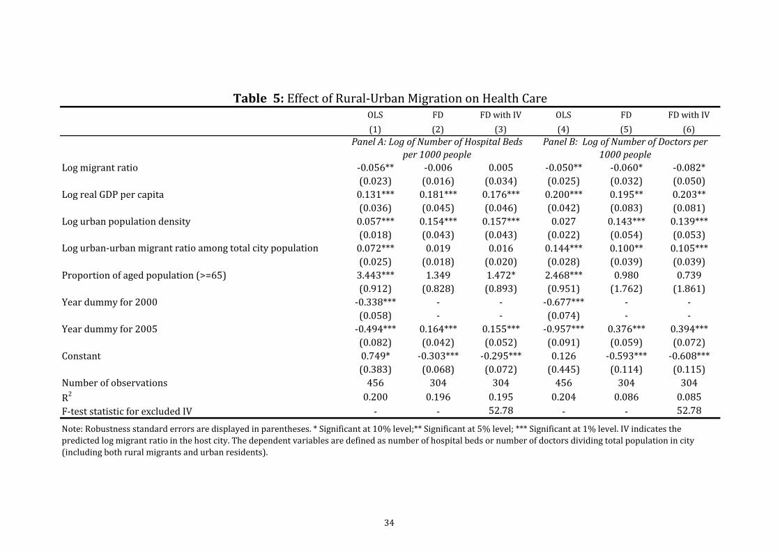
OLS FD FD with IV OLS FD FD with IV (1) (2) (3) (4) (5) (6)
Log migrant ratio -0.056** -0.006 0.005 -0.050** -0.060* -0.082*(0.023) (0.016) (0.034) (0.025) (0.032) (0.050)
Log real GDP per capita 0.131*** 0.181*** 0.176*** 0.200*** 0.195** 0.203**(0.036) (0.045) (0.046) (0.042) (0.083) (0.081)
Log urban population density 0.057*** 0.154*** 0.157*** 0.027 0.143*** 0.139***(0.018) (0.043) (0.043) (0.022) (0.054) (0.053)
Log urban-urban migrant ratio among total city population 0.072*** 0.019 0.016 0.144*** 0.100** 0.105***(0.025) (0.018) (0.020) (0.028) (0.039) (0.039)
Proportion of aged population (>=65) 3.443*** 1.349 1.472* 2.468*** 0.980 0.739(0.912) (0.828) (0.893) (0.951) (1.762) (1.861)
Year dummy for 2000 -0.338*** - - -0.677*** - -(0.058) - - (0.074) - -
Year dummy for 2005 -0.494*** 0.164*** 0.155*** -0.957*** 0.376*** 0.394***(0.082) (0.042) (0.052) (0.091) (0.059) (0.072)
Constant 0.749* -0.303*** -0.295*** 0.126 -0.593*** -0.608***(0.383) (0.068) (0.072) (0.445) (0.114) (0.115)
Number of observations 456 304 304 456 304 304R2 0.200 0.196 0.195 0.204 0.086 0.085F-test statistic for excluded IV - - 52.78 - - 52.78
Panel B: Log of Number of Doctors per 1000 people
Note: Robustness standard errors are displayed in parentheses. * Significant at 10% level;** Significant at 5% level; *** Significant at 1% level. IV indicates the predicted log migrant ratio in the host city. The dependent variables are defined as number of hospital beds or number of doctors dividing total population in city (including both rural migrants and urban residents).
Panel A: Log of Number of Hospital Beds per 1000 people
Table 5: Effect of Rural-Urban Migration on Health Care
34

OLS FD FD with IV (1) (2) (3)
Dependent Variable - Log of Number of Passengers Per BusLog migrant ratio 0.098** 0.105** 0.169
(0.044) (0.050) (0.136)Log real GDP per capita -0.076 0.023 -0.008
(0.058) (0.075) (0.085)Log urban population density 0.145** 0.293 0.268
(0.058) (0.241) (0.239)Log urban-urban migrant ratio among total city population 0.001 0.022 0.005
(0.047) (0.046) (0.051)Log total land areas of the city 0.110** 0.079 0.049
(0.048) (0.159) (0.162)Log number of taxis 0.106*** 0.013 0.024
(0.026) (0.034) (0.042)Year dummy for 2000 -0.820*** - -
(0.104) - -Year dummy for 2005 -0.739*** 0.792*** 0.760***
(0.127) (0.114) (0.111)Constant 5.079*** -0.761*** -0.718***
(0.693) (0.164) (0.155)Number of observations 438 292 292R2 0.312 0.399 0.394F-test statistic for excluded IV - - 51.47
Table 6: Effect of Rural-Urban Migration on Public Transportation
Note: Robustness standard errors are displayed in parentheses. * Significant at 10% level;** Significant at 5% level; *** Significant at 1% level. IV indicates the predicted log migrant ratio in the host city. Since 6 cities have missed bus/taxi information in 1990, the city sample reduces to 146 for this analysis.
35

FD FD with IV (1) (2) (3) (4) (5)
Log migrant ratio 0.266*** 0.187*** 0.128* -0.079 0.021(0.056) (0.063) (0.066) (0.099) (0.222)
Log Proportion of males aged 15-40 among total city population - 1.511*** 0.965* 0.033 -0.107- (0.539) (0.552) (0.687) (0.700)
Log real GDP per capita - - 0.189* 0.256 0.228- - (0.107) (0.206) (0.207)
Log urban population density - - 0.064 0.036 0.067- - (0.045) (0.185) (0.195)
Log urban-urban migrant ratio among total city population - - 0.122* 0.150 0.130- - (0.064) (0.112) (0.120)
Log employment rate - - -0.779 0.158 0.022- - (0.599) (0.588) (0.644)
Year dummy for 2000 0.382*** 0.508*** 0.112 - -(0.111) (0.115) (0.169) - -
Year dummy for 2005 0.682*** 0.988*** 0.716* 0.253 0.238(0.097) (0.134) (0.382) (0.329) (0.320)
Constant 1.651*** 3.465*** 1.136 -0.133 -0.077(0.181) (0.660) (1.377) (0.322) (0.341)
Number of observations 453 453 453 302 302R2 0.158 0.184 0.221 0.017 0.013F-test statistic for excluded instrument - - - - 42.27Panel B: Controlling for log gini coefficent (sample cities reduce to 64)Log migrant ratio 0.377*** 0.228** 0.211* -0.014 0.149
(0.090) (0.105) (0.117) (0.154) (0.362)Log gini coefficient 0.136 0.067 0.024 -0.438 -0.337
(0.415) (0.417) (0.444) (0.552) (0.562)Number of observations 192 192 192 128 128R2 0.244 0.278 0.313 0.060 0.053F-test statistic for excluded instrument - - - - 16.53Panel C: Not Controlling for log gini coefficent, bus use 64 city-sampleLog migrant ratio 0.379*** 0.229** 0.212* 0.008 0.185
(0.090) (0.105) (0.116) (0.149) (0.341)Number of observations 192 192 192 128 128R2 0.243 0.278 0.313 0.056 0.046F-test statistic for excluded instrument - - - - 18.76Note: Robustness standard errors are displayed in parentheses. * Significant at 10% level;** Significant at 5% level; *** Significant at 1% level. IV indicates the predicted log migrant ratio in the host city. The dependent variable-crime rate- is defined as log number of prosecuted criminal cases per 1000 persons (including both rural migrants and urban residents). Since one city have missed crime information in 2005, the city sample reduces to 151 for crime equation. Panel B gives the results with additional control for Log Gini coefficients. Gini coefficients in 1990 and 2000 are calculated based on the Urban Household Surey data and Gini coefficients in 2005 are taken from 2005 mini-Census. To keep the consistent cities with Gini information over three years, the sample size further reduces to 64 cities for each year. To make the comparison, in Panel C, we include the regression results based on 64 city-sample without control for Gini coefficients.
Table 7: Effect of Rural-Urban Migration on Crime RatesOLS
Panel A : Dependent Variable: Log of Crime Rates
36

Single Regression IV
Coefficient for Log Migrant Ratio (1) (2) (3) (4) (5)Teacher/Student Ratio in Primary Schools 0.032 -0.001 -0.001 -0.001 -0.021
(0.042) (0.029) (0.029) (0.029) (0.030)Teacher/Student Ratio in Middle Schools 0.066** 0.052** 0.052** 0.052** 0.047*
(0.028) (0.026) (0.026) (0.026) (0.027)Number of Hospital per 1000 person 0.005 -0.055 - -0.055 -0.061*
(0.034) (0.034) - (0.034) (0.036)Number of Doctor per 1000 person -0.082* - -0.070 -0.070 -0.081
(0.050) - (0.079) (0.079) (0.082)Passenger per Bus 0.169 0.146** 0.146** 0.146** 0.106
(0.136) (0.074) (0.074) (0.074) (0.077)Crime Rates 0.021 -0.045 -0.045 -0.045 -
(0.222) (0.188) (0.188) (0.188) -
Table 8: Robustness Check: Seemingly Unrelated Regression Results
SURE with IV
Note: Standard errors are displayed in parentheses. * Significant at 10% level;** Significant at 5% level; *** Significant at 1% level. In each panel, five FDIV regressions for different outcomes are jointly estimated by using Seemingly Unrelated Regression with controls of same independent variables as those included in Tables 2-5. To simplify, only coefficients of log migrant ratio are presented in this table. Columns (4) and (5) exclude crime regression. The difference between columns (2) and (3), (4) and (5) is to choose number of hospital or number of doctor per 1000 person to be the indicator for health care.
37

FD FD with IV FD FD with IV FD FD with IV FD FD with IVLog migrant ratio 0.002 -0.020 -0.059* -0.105** 0.161*** 0.344*** 0.037 -0.062
(0.017) (0.035) (0.035) (0.052) (0.060) (0.132) (0.111) (0.219)
Log migrant ratio * Year dummy for 2005 -0.032 0.118 -0.003 0.107 -0.215** -0.759*** -0.480** 0.406(0.034) (0.113) (0.061) (0.120) (0.084) (0.232) (0.204) (0.628)
Number of observations 304 304 304 304 292 292 302 302R2 0.198 - 0.086 - 0.412 - 0.035 -
F-test statistic for excluded IV (Log migrant ratio) - 32.74 - 32.74 - 32.13 - 28.34F-test statistic for excluded IV (interaction term) - 7.90 - 7.90 - 7.61 - 8.64
Hospital beds Doctors Panssegers per bus CrimeTable 9: Time Varying Effect of Migration Inflow on Social Outcomes
38

Figure 1: Local government share of total fiscal expenditure: 1953-2005
Source: China Statistical Yearbook, 2001 and 2006
2040
6080
Loca
l gov
. sha
re o
f fsi
cal e
xpen
ditu
re (%
)
1953 1958 1963 1968 1973 1978 1983 1988 1993 1998 2003year
39

Figure 2: Unconditional Relationship between the Dependent Variables and Migrant ratio
-3.5
-3-2
.5-2
-3.5
-3-2
.5-2
-8 -6 -4 -2 0 -8 -6 -4 -2 0
1990 2000
2005 Total
Log
(Tea
cher
/Stu
dent
)
Log Migrant RatioGraphs by year
Primary School
.51
1.5
22.
5.5
11.
52
2.5
-8 -6 -4 -2 0 -8 -6 -4 -2 0
1990 2000
2005 Total
Log
(Hos
pita
l Bed
s/Po
pula
tion)
Log Migrant RatioGraphs by year
Hospital Beds
24
68
24
68
-8 -6 -4 -2 0 -8 -6 -4 -2 0
1990 2000
2005 Total
Log
(Pas
seng
er p
er B
us)
Log Migrant RatioGraphs by year
Passengers per Bus
-3.5
-3-2
.5-2
-3.5
-3-2
.5-2
-8 -6 -4 -2 0 -8 -6 -4 -2 0
1990 2000
2005 Total
Log
(Tea
cher
/Stu
dent
)
Log Migrant RatioGraphs by year
Secondary School
01
20
12
-8 -6 -4 -2 0 -8 -6 -4 -2 0
1990 2000
2005 Total
Log
(Doc
tors
/Pop
ulat
ion)
Log Migrant RatioGraphs by year
Number of Doctors
-20
24
-20
24
-8 -6 -4 -2 0 -8 -6 -4 -2 0
1990 2000
2005 Total
Log
(# o
f Crim
e P
rose
cute
d/P
opul
atio
n)
Log Migrant RatioGraphs by year
Crime Rate
40
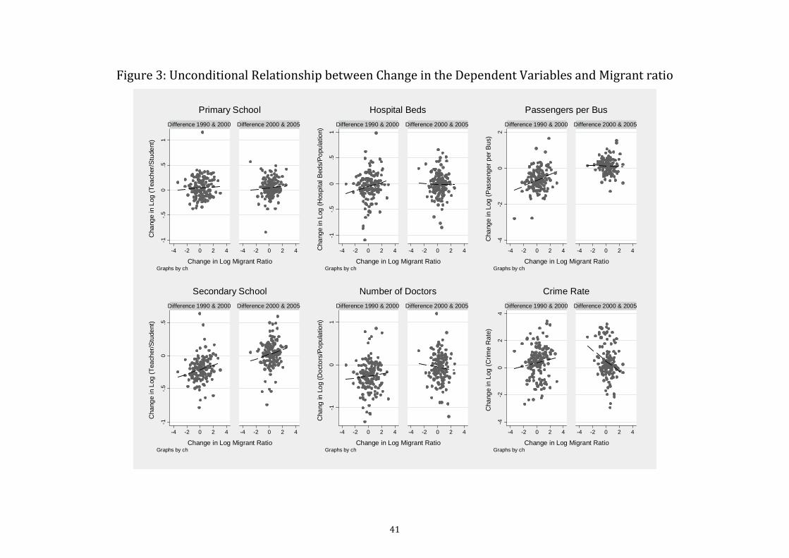
Figure 3: Unconditional Relationship between Change in the Dependent Variables and Migrant ratio
-1-.5
0.5
1
-4 -2 0 2 4 -4 -2 0 2 4
Difference 1990 & 2000 Difference 2000 & 2005
Cha
nge
in L
og (T
each
er/S
tude
nt)
Change in Log Migrant RatioGraphs by ch
Primary School
-1-.5
0.5
1
-4 -2 0 2 4 -4 -2 0 2 4
Difference 1990 & 2000 Difference 2000 & 2005
Cha
nge
in L
og (H
ospi
tal B
eds/
Pop
ulat
ion)
Change in Log Migrant RatioGraphs by ch
Hospital Beds
-4-2
02
-4 -2 0 2 4 -4 -2 0 2 4
Difference 1990 & 2000 Difference 2000 & 2005
Cha
nge
in L
og (P
asse
nger
per
Bus
)
Change in Log Migrant RatioGraphs by ch
Passengers per Bus
-1-.5
0.5
-4 -2 0 2 4 -4 -2 0 2 4
Difference 1990 & 2000 Difference 2000 & 2005
Cha
nge
in L
og (T
each
er/S
tude
nt)
Change in Log Migrant RatioGraphs by ch
Secondary School
-10
1
-4 -2 0 2 4 -4 -2 0 2 4
Difference 1990 & 2000 Difference 2000 & 2005
Cha
ng in
Log
(Doc
tors
/Pop
ulat
ion)
Change in Log Migrant RatioGraphs by ch
Number of Doctors
-4-2
02
4
-4 -2 0 2 4 -4 -2 0 2 4
Difference 1990 & 2000 Difference 2000 & 2005
Cha
nge
in L
og (C
rime
Rat
e)
Change in Log Migrant RatioGraphs by ch
Crime Rate
41
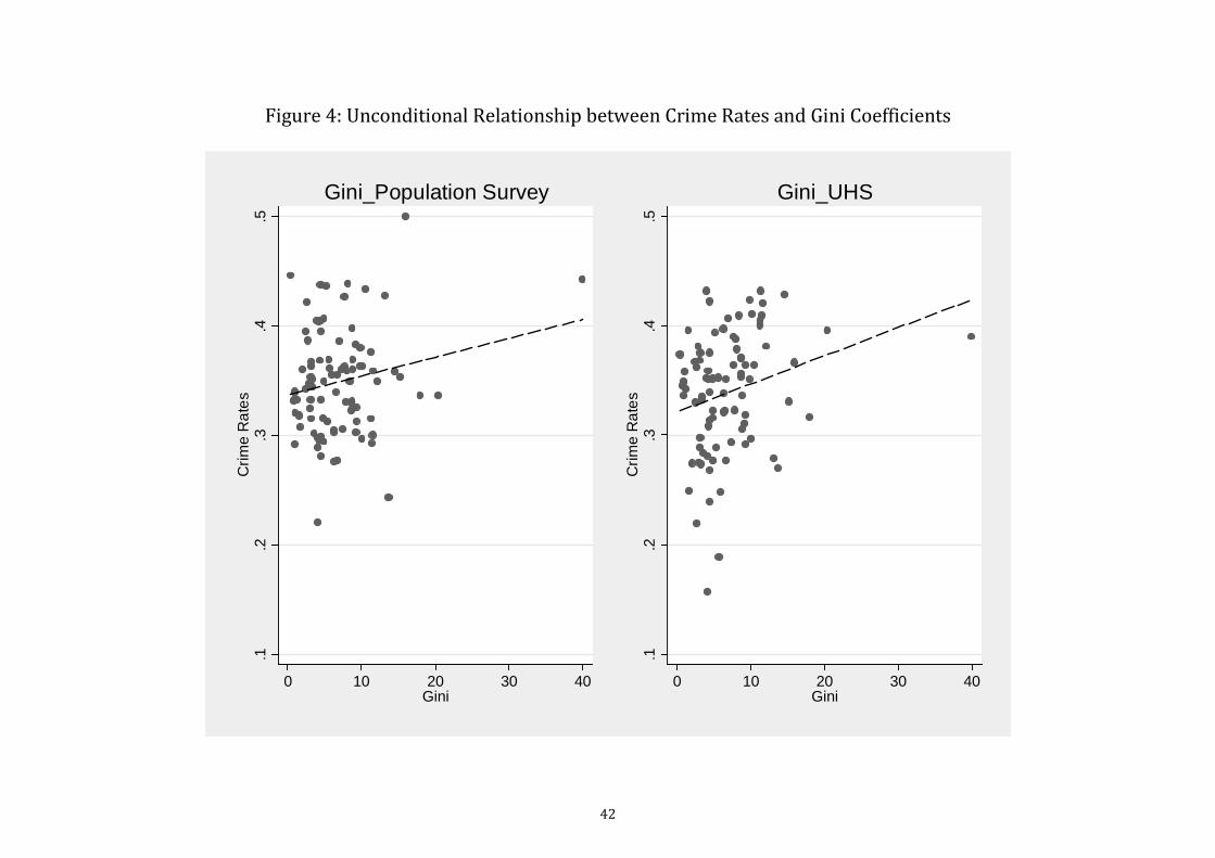
Figure 4: Unconditional Relationship between Crime Rates and Gini Coefficients
.1.2
.3.4
.5C
rime
Rat
es
0 10 20 30 40Gini
Gini_Population Survey
.1.2
.3.4
.5C
rime
Rat
es
0 10 20 30 40Gini
Gini_UHS
42

1990 2000 2005Panel A: Push factor
Land per capita -2.810* 4.622 -5.421***(1.615) (3.109) (1.057)
Land per capita2 1.655** -3.392* 0.531***(0.773) (1.794) (0.119)
Net income per capita 0.000 0.003** -0.000(0.001) (0.001) (0.001)
Areas of disaster 0.000 0.027*** 0.001***(0.000) (0.005) (0.001)
Total power of agricutural machinery 0.000 -0.002*** -0.001***(0.000) (0.001) (0.000)
Constant 1.466* -1.165 12.699***(0.765) (1.576) (2.834)
Number of observations 28 28 30R2 0.244 0.588 0.491Panel B: Pull factor
Distancekj -0.636* -0.750*** -0.660**(0.375) (0.188) (0.267)
Distancekj2 0.216 0.230*** 0.211**
(0.132) (0.063) (0.093)Interactions between Distance and Province dummies Yes Yes YesInteractions between Distance2 and Province dummies Yes Yes YesDummies for province Yes Yes YesConstant 0.411* 0.569*** 0.485***
(0.229) (0.123) (0.167)Number of observations 1,049 2,162 1,442R2 0.577 0.555 0.500Note: Robustness standard errors are displayed in parentheses. * Significant at 10% level;** Significant at 5% level; *** Significant at 1% level. IV indicates the predicted log migrant ratio in the host city. The dependent variable-crime rate- is defined as log number of prosecuted criminal cases per 1000 persons (including both rural migrants and urban residents). Hainan and Sichuan missed for 1990 and 2000 regressions due to the incomplete information.
Appendix Table A1: Results from Regressions Used to Construct the Instrument
Dependent variable: out-migration rate from source province k
Dependent variable: migration probability from source province k to city j
43
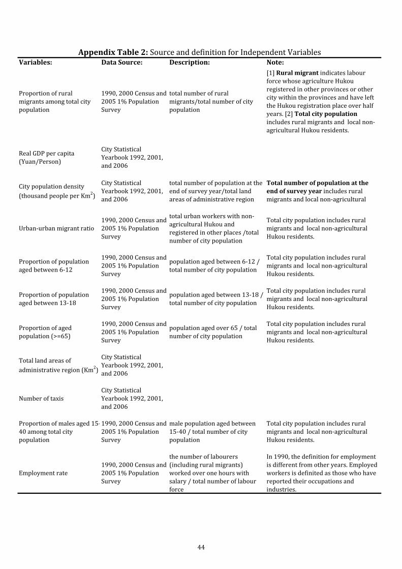
Variables: Data Source: Description: Note:
Proportion of rural migrants among total city population
1990, 2000 Census and 2005 1% Population Survey
total number of rural migrants/total number of city population
[1] Rural migrant indicates labour force whose agriculture Hukou registered in other provinces or other city within the provinces and have left the Hukou registration place over half years. [2] Total city population includes rural migrants and local non-agricultural Hukou residents.
Real GDP per capita (Yuan/Person)
City Statistical Yearbook 1992, 2001, and 2006
City population density (thousand people per Km2)
City Statistical Yearbook 1992, 2001, and 2006
total number of population at the end of survey year/total land areas of administrative region
Total number of population at the end of survey year includes rural migrants and local non-agricultural
Urban-urban migrant ratio 1990, 2000 Census and 2005 1% Population Survey
total urban workers with non-agricultural Hukou and registered in other places /total number of city population
Total city population includes rural migrants and local non-agricultural Hukou residents.
Proportion of population aged between 6-12
1990, 2000 Census and 2005 1% Population Survey
population aged between 6-12 / total number of city population
Total city population includes rural migrants and local non-agricultural Hukou residents.
Proportion of population aged between 13-18
1990, 2000 Census and 2005 1% Population Survey
population aged between 13-18 / total number of city population
Total city population includes rural migrants and local non-agricultural Hukou residents.
Proportion of aged population (>=65)
1990, 2000 Census and 2005 1% Population Survey
population aged over 65 / total number of city population
Total city population includes rural migrants and local non-agricultural Hukou residents.
Total land areas of administrative region (Km2)
City Statistical Yearbook 1992, 2001, and 2006
Number of taxisCity Statistical Yearbook 1992, 2001, and 2006
Proportion of males aged 15-40 among total city population
1990, 2000 Census and 2005 1% Population Survey
male population aged between 15-40 / total number of city population
Total city population includes rural migrants and local non-agricultural Hukou residents.
Employment rate 1990, 2000 Census and 2005 1% Population Survey
the number of labourers (including rural migrants) worked over one hours with salary / total number of labour force
In 1990, the definition for employment is different from other years. Employed workers is definited as those who have reported their occupations and industries.
Appendix Table 2: Source and definition for Independent Variables
44


