
AD-AI04 14 01H10 STATE WINlY COLL"MU DEPT OF GE0I*TIC SCIZNCL pie 8/bTHE USE OF FINITE ELEMENTS IN PH4YSICAL SEOOESY,Iu)
NCAS10 APR &I P NEISbA. F19YZS-79-C-00om
F4I.ASPE DOS-313 AFGL-TR-81-0114 "L

AFGL-TR-81-0114
THE USE OF FINITE ELEMENTS IN PHYSICAL GEODESY
PETER MEISSL
DEPARTMENT OF GEODETIC SCIENCETHE OHIO STATE UNIVERSITYRESEARCH FOUNDATIONCOLUMBUS, OHIO 43210
APRIL 1981
SCIENTIFIC REPORT NO. 7
APPROVED FOR PUBLIC RELEASE; DISTRIBUTION UNLIMITED
~'AIR FORCE GEOPHYSICS LABORATORYAIR FORCE SYSTEMS COMMANDUNITED STATE AIR FORCEHANSCOM AFB, MASSACHUSETTS 01731
• ' . ,h, i,

Qualified requestors may obtain additional copies fromthe Defense Documentation Center. All others should
apply to the National Technical Information Service.
PI.7

UnclassifiedSECURITY CLASSIFICATION OF THIS PAGE (mien Deta Entered)
RT PAGE READ INSTRUCTIONSREPORT DOUMENTTION PABEFORE COMPLETING FORM
-2.GOVT ACCESSION NO. 3 RECIPIENT'S CATALOG NUMBER
AFG TR-81-0114; ___
4. TITLE (and Subtitle) S. TYPE OF REPORT I PERIOD COVERED
THE USE OF FINITE ELEMENTS IN PHYSICAL GEODESY Scientific Report No. 7
6 PERFORMING ORG. REPORT NUMBER
Report No. 3137 AUTHOR(e) 6. CONTRACT OR GRANT NUMBER(.)
PETERIMEISSL F19628-79-("-0075
9. PERFORMING ORGANIZATION NAME AND ADDRESS 10. PROGRAM ELEMENT. PROJECT, TASK
Department of Geodetic Science AREA & WORK UNIT NUMBERS
The Ohio State University 6210WF
Columbus, Ohio 43210 76OOb3AI.
1 I. CONTROLLING OFFICE NAME AND ADDRESS 12. REPORT. DATE
Air Force Geophysics Laboratory . April 1981Hanscom AFB, Massachusetts 01731 .. IS. NUMWAOF PAGES
Contract Monitor - Bela Szabo - IW Pages 20914. MONITORING AGENCY NAME & ADDRESS(If different from Controlling Office) IS. SECURITY CLASS. (of thie report;
, -. Unclassified- Ia. DECLASSIFICATION, DOWNGRADING
SCHEDULE
16. DISTRIBUTION STATEMENT (of thie Report)
Approved for public release; distribution unlimited
17. DISTRIBUTION ST. tENT (of abstract entered In Block 20, If different from Report)
IS. SUPPLEMENTARY TES
T9 KEY WOROS 'Con(inue on reverse side If neceeitry and Identify by block number)
Physical geodesy, Finite elements, Spherical harmonics, Surface layter,Splines, Stokes formula, Vening Meinesz formula, Multipoles, Free boundaryvalue problem, Hermite cubics, Computational efficienty, and Comparison ofmethods.
Z0 ABSTRACT (Continue on re.tree side if neceseery end Identify by block number)
-Currently used methods of computational physical geodesy are compared withrespect to their efficiency during production runs on a computer. Thesemethods include: (1) Least Squares adjustment with respect to sphericalharmonics: (2) Surface layers, buried masses and related methods; (3) Leastsquares collocation; (4) Representation of the potential by spline functions;(5) Explicit integral formulas. As an alternative, the feasibility ofapplying the finite element method to the fundamental problems of physicalgeodesy is investigated. The methods listed under (1)-(4) can be dramatically
DD I JAN3 14731,. UnclassifiedSECURITY CLASSIFICATION OF THIS PAGE (When Dae Entered)
-'.-- .- 1

SECURITY CLASSIFICATION or
THIS PAGE(Wh.. Ote natered)
.speeded up if the distribution of data and weights satisfies certain symetry-requirements which are rather stringent. Method (5) relies altogether on aspecial type and distribution of data. In the absence of data homogeneity andregularity, the finite element method is asymptotically superior with respectto computational efficiency. Let N denote the number of parameters necessaryto describe the variation of the potential on the reference surface. The com-putational effort associated with methods (1)-(4) grows proportional to N3.That one resulting from finite elements grows proportional t0 N. The constantsof proportionality are, however, unfavorable for the finite element method.Hence its superiority comes through only for large values of N, which, in caseof a global solution, corresponds to data averaged over 2 x 2 blocks.
SECURITY CLASSIFICATIO4N OF THIS PAGEtWhen Data Entered)
FOREWORD
This report has been prepared by Peter Meissl, Professor for
Theoretical Geodesy at the Technical University in Graz. Part of the
work, in particular that one involving a large computer, was carried
out during a 3-month research period at the Department of Geodetic
Science, at The Ohio State University. The work was done under Air
Force Contract No. F19628-79-C-0075, The Ohio State University Research
Foundation, Project No. 711715, Project Supervisor, Urho A. Uotila,
Professor, Department of Geodetic Science. The contract covering this
research is administered by the Air Force Geophysics Laboratory (AFGL),
Hanscom Air Force Base, Massachusetts, with Bela Szabo, Project Scientist.
AcC9S~flFor\I'T!S 0-A&
A U5t I 2 f 1
DP .. ...
AV" ::: L Y "'l

ACKNOWLEDGEMENTS
The author wishes to thank Professor U.A. Uotila for valuable
advice. Also the discussions with 0. Colombo are gratefully
acknowledged. Very efficient help in problems of computer-job-control,
interactive use of computers, and telecommunication, was received from
Lenny A. Krieg. My co-worker B. Hofmann-Wellenhof shared with me the
workload of compiling the final report. The manuscript was assembledand plotted with the help of a self-made text-editing system. The system
is being developed by my co-workers N. Bartelme and H. Zach. Unfortunately
the programs supporting indexing, Greek lettering, and mathematicalnotation became available at a time when most of the report was already
processed. Chapter 7 gives a sample of the full capabilities of the
sys tern.
___________

vii
Contents
1. Introduction and outline of results
2. Review of various methods 6
2.1. Spherical harmonics 7.. .... 7
2.2. Surface layer representation and related methods 9
2.3, Least squares collocation .. ........ 10
2.3.!. Krarup's proposal ..
2.3.2. Least squares collocation using unknown parameters 12
2.4. Finite elements 3......3
2.5 Spline functions ...... 16
2.6 Approximate explicite Green's functions .. 19
2 7 Exploiting rotational or translational symmetries 20
2.7.1. Invariance of normal equations under a group of
transformations 0........ ....... 22.7.2. Outline for the case of rotational symmetry around an
axis ............ .... 222.7.3. The effort of the TASC group .... 232.7.4. Rauhala's array algebra 9.... ..... 2
3. Outline of the finite element aporoach .. .. .. .. 33
3.1. Hermite-cubic representation of the field 33
3.1.1. The four basis functions for the unit interval 33
3.1 2. Interval of length h .......... 34
3.1.3. Bicubic polynomial in a rectangle with sides a, b 35
3.1.4. Tricubic polynomials in a box with sides a, b, c 36
3.1.5. C' continuity across element boundaries .. 36
3.1.6. Compound elements 3............38
3.2. Shape functions ............... 40
3.3. Conirlbution of the field to the normal equations 41
3.3.1. Reasons for excluding the Ritz method .... 41
3.3.2. The least squares contribution of the field .. 45
3.4. Detailed instructions for computer implementation 48
3.4.1. The partial normals of a simple quad s...
34.2. Partial normals of a compound element .. 58
3.5. More general basis functions ........ 63
3.6. Elements extending to infinity in one direction .... .. 67
3.7. The outer zone 71

viii
3.8. Local data deficiencies ...... 78
4. Estimation of computation time 81
4.1. Nested dissection and Helmert blocking 81
4.2. Global solution 874.3. The remote zone effect ...... 1014.4. Detailed soluEion in a strip. 1014.5. Rectangular region 7......17
4.6. Further effort to cut down the computation time. .,. 111
S. A proposal for a numerical solution of the free boundaryvalue problem ............ ...... 117
5.1. Isoparametric elements ........ ...... 117
5.2. Approaching the free boundary value problem of physical
geodesy .. ........ .... .. 125
6. Computer experiments for 2-dimensional problems .... .. 129
6.1. Purpose and scope 9........ .... 12
6.2. Parameters distinguishing the experiments .. 132
6.3. Detailed results for two experiments 1..38
6.3.1. An experiment using comparatively large elements 138
6.3.2. An experiment using comparatively small elements 1656.4. Summary of other experiments 1..77
6.4 1 Experiments using bicubics 1.. .. 776.4.2. Experiments using biquintics 179
4 6.4.3. Discussion .......... 1816.4.4. A word on the Computer programs 182
6.4.5. Further desirable experimerts 182
7. A proposed hybrid method .. 184
7.1. Revision of the surface layer method 184
7.2. Multipole layer .......... .... 184
7.3. Multipole layers on the sphere .......... 186
Appendix A. Computational effort associated with the
partial reduction of a profiled system of normal
equations .................... 19
References 14...................4
-
1. Introduction and outline of results
This report pursues two goals. These are
(I) A comparison of currently used methods in computational physical
geodesy. This was the primary desire of the contractor.
(2) A feasibility study on the use of the finite element method for the
numerical solution of the fundamental problem of physical geodesy. This
was the primary desire of the author.
The fundamental problem of physical geodesy is the simultaneous
determination of the earth's figure and potential from geometric and
gravimetric measurements. The numerical solution requires a finite
parameterization of the potential and - in case of a sophisticated
approach - also of the earth's figure.
A comparison of various methods for the detailed representation of
the earth's gravity field has recently been given by Tscherning (1979).
His confirmed impression is that there is a number of competing methods
performing about equally .ell as far as the quality of results is
concerned.
In chapter 2 of the present report various methods currently used
to approach the problem of the determination of the earths figure and
potential were examined from the viewpoint of computational efficiency.
Methods like collocation, surface layer, buried masspoints, Bjerhammar's
method, lead to a fully occupied linear system of equations to be
solved. The effort to solve such a system is proportional to N3, where N
is the number of equations. Breakdown due to OSU-CPU Limes exceeding 100
hours occurs at about N = 10,000 (this corresponds to a surface layer
solution with 20 x2O blocks near the equator)
If the pattern of data and weights shows rotational symmetry,
great savings in computation time can be obtained by using techniques
. . . . t

2-
based on discrete Fourier transform of block circulant matrices. This
has been shown by Colombo T80). The author feels Lhat Colombo's
approach is currently the best one if an essentially nonredundant set of
surface data is employed. Such a set is for example given by I'xl ° block
averages of gravity anomalies. Although the quality of such block
averages varies greal!y between areas, the assumption of equal weights
will not cause too much harm to the estimated parameters, because there
is no problem of adjusting redundant data. The system must take what it
gets and has no choice to balance poor anomalies against better
observations. Of course, the accuracy estimates obtained from such a
procedure are very problematic.
Similar things may be said about GEOFAST developed by TASC. The
asymptotic speed is even proportional to N log N. The gain in speed is
paid for by restricting applications to data distributed regularly on a
line or within a rather small plane rectangle. Some possible trouble
spots are indicated in chapter 2. One of them is concerned with
trcnsporting a covariance from the sphere to the plane. Harmonicity gets
lost thereby. it would also be interesting to have some idea on the
proportionality factor in front of the N log N term estimating the CPU
time.
Chapters 3 to 6 document a feasibility study on the use of the
finite element method in physical geodesy. This method leads to a sparse
set of equations whose solution requires an effort proportional to NT,
where N has the same meaning as above. Unfortunately the constant of
proportionality is large. The break even point between the surface layer
and finite elements in a global solution is estimated to be around 20x20
blocks. For smaller blocks finite elements are faster, for larger ones
the surface layer is faster. The effort for a global solution based on
l7xi0 gravity anomaly data is estimated at 700 OSU CPU hours. A special
technique exploiting the remote zone effect could reduce this to about
250 hours (the surface layer method would require 15,000 hours). An
effort of 250 OSU CPU hours is considered too large. Several reruns
-3-
would be necessary before a satisfactory choice of weights is found
A~lhough there exist computers, as for example the ILLIAC V7, on which
the CPU time could be cut by a factor of about 64, the problem apoears
too large for one individual researcher or a small research group,
Fortunately, the remote zone effect allows to compute local
solutions. The report will give an estimate for the calculation of a
detailed potential in an equatorial strip (6.5 hours) and in a
rectangular area of size 32'x640 (covering e.g. the contiguous US). In
the iatter case 30'x 3O' data were assumed. CPU Lime was estimated at 20
OSU hours. By a sophisticated use of the remote zone effect this can
probably be lowered to 6 hours. This compares favorably with a surface
layer solution requiring about 70 hours.
The finite element method does not rely on any regular pattern of
observation and weights. (Regularity could be exploited in the some way
as with the other methods. The additional saving in CPU time would,
however, not be dramatic.) In areas where the field shows much detail,
smaller elements may be chosen. Redundant data, as for example gravity
anoma!ies plus geoid heighLs, pose no problem. The method offers also
disadvantages. Harmonicity of the calculated field is only approximate.
The programming effort for an efficient computer implementation is
considerable.
The finite element method !oses much of its efficiency if the data
are not local. Local data are composed of measurements taken in a way
that one measurement involves only a single point or a small vicinity of
a point. A vicinity of a point is considered small if it contains only a
small number of the finite elements in its interior. A more precise
definition of the locality of a measurement would be that its
contribution to the normal equations must not destroy the sparsity
pattern resulting from a field representation by means of finite
elements. ata obtained by integrating over an unknown orbit are not
local. Neither are misclosures of large inertial navigation loops There
..... .. • : __ .. _---. L 2 ,T..: .. .. ' .t ','' '

-4-
are, however, ways to ,)corporate orbits at higher altitudes in an
efficient way
The finite element method lends itself to Helmert blocking, or its
modern vcr:anL, nested dissection. Calcuiations For subregions (nations,
continents) could be deiegated. Junction equations could be combined at
a higher level, very much in the same way as this is done :n continental
network adjustment.
Chapter 6 documents a number of test calculations They were
carried out with the following gocis.
(I) To see whether the Ritz-, or the Trefftz-, or the old fashioned
east squares principe should be used (The lolter is recommended for
the specific needs of physical geodesy).
(2) To see whether the use of cubic polynom:als is sufficient, or
whether quint;c or even higher degree polynomials are needed. (Cubics
are sufficient, quintics are already hopeless from the CPU time point of
view).
(3) To see whether a certain type of element partition making a best
possible use of the 'attenuation with altitude effect" can be employed.
(The outcome was satisfactory).
(4) To find an appropriate representation of the field in the remote
outer space of the earth (Specially designed elements of infinite size
and appropriately chosen shape functions performed well in this
respect).
(5) To get an idea how the observational weights should be balanced
against the weights apcled to the equations enforcing the approximate
fulfillment of Lan!ace's equation. (Reasonable weighLs were found by
experiment. More ins~gnt wouid be desirab~e)

(6) To see whether a combination solution of surface gravity values and
satellite derived harmonics is possible. (The answer is yes, but
additional tests are necessary to identify procedures preventing a
substantial increase in CPU time).
The experiments were carried oul in 2 dimensions in order to save CPU
time. Small scale 3-dimensional calculations are desirable, but there
was no time yet to perform them.
In the authors opinion the finite element method has a place in
physical geodesy. It is very likely that a proposal by Junkins (1979)
will be accepted, suggesting to use a finite element representation of a
completely known potential for the purpose of rapid recalculation in
real time application and also otherwise. The authors feeling is that
finite elements are also useful to porameterise an unknown potential
during an estimation procedure. However, the method must be cultivated
somewhat more before a large scale effort is attempted. At the end of
the research period covered by this report, the author began to look
into a hybrid method which combines finite elements with a surface layer
of multipoles. Some preliminary statements on this envisioned method are
given in chapter 7. Another feature which makes finite elements
attractive is the possibility to attack in a head-on way the free
boundary value problems of physical geodesy. Some ideas how this could
be accomplished are found in chapter S.
j 1

2. Review of various methods
Consider an earth-centered and earth-fixed coordinate system. Choose a
convenient reference potential, e.g. that one of an equipotential
ellipsoid, or one obtained from a truncated spherical harmonics
expansion. The normal potential is assumed to completely absorb the
rotational effect. Hence the disturbing potential V is purely
gravitational. In outer space it satisfies Laplace's equation
AV= 0 (2.1)
Laplace's equation represents a local law. In order to evaluate the
second order differential operator at a certain location x, we need only
information on V in a local neighborhood of x.
The purpose of physical geodesy is the determination of the earths
surface and potentiai from geodetic measurements. There is hardly a need
to point out that the measurements are indirect, and that it is
therefore necessary to represent surface and potential in terms of a
number of unknown parameters. Because computers perform only finitely
many operations in a finite amount of time, the number of parameters
must be finite.
The choice of an appropriate set of parameters is highly
nontrivial. Factors to be taken into account are:
(*) Type of ajpplication, e.g., local improvements or global
corrections to the field.
C*) Type and distribution of measurements, in particular,
homogeneous or heterogeneous sets of data.
(*) Mathematical simplicity and elegancy. Simple setups are
easier to program. Debugging the programs is less time
consuming.

7
00 Computer time during production runs.
Let us restrict attention to the potential, forgetting temporarily the
parameters describing the unknown reference surface. Let us review and
discuss representations of the potential that have been used by
geodesists. Our main emphasis will be on the lost item listed above,
i.e. computational efficiency during production runs.
2.1. Spherical harmonics.
They satisfy Laplace's equation automatically. The trace functions with
respect to the unit sphere are the surface spherical harmonics. They are
the eigenfunctions of any rotation invariant operator on the sphere.
Confer Mueller (1966), Meissl (1971a), Robertson (1978), Freeden (1979)
for extensive discussions. Spherical harmonics provide great theoretical
insight. They lead to the concept of the power spectrum of the
potential'. If a problem can be formulated in a way that rotation
symmetry is preserved, then spherical harmonics are also of great
computational advantage. In this context recent papers by
Freeden (1978), (1979) are pointed out where methods for numerical
integration of functions defined on the sphere are specified. The
formulas are related to the familiar Gaussian quadrature formulas for
intervals, i.e. they rely on a weighted average of function values at a
set of discrete points. It is likely that the formulas can be extended
to functions discretized in terms of block averages.
Spherical harmonics are widely used in satellite geodesy. At
satellite altitudes of 1000 km and above, the potential is sufficiently
attenuated to be properly represented by a spherical harmonics expansion
of moderately large degree (N = 20-30, or so).
-.. 7 7

Let us now assume that 4e are dealing with a problem invoivr g o
neterogeneous set of data, suggesEng a east squares setup by variation
of parameters. Then one Particular property of spherical harmonics
counteracts comouto aonai efficiency. This oroperty of spherical
harmon:cs is that they cre nonzero aimost everywhere No function
different from he zero function can satisfy Lapiace's equatlio and, at
the same time, vanisn in a part of he domain having nonzero measure.
Thus spherical harmonics fail to nave a local support. If the disturbing
potential is represented in terms of spherical harmonics as
N +L
V(X) Z .ciLjHLX (2.2./
and if a local measurement leads to a linear functional L(V) involving
only points in a small vicinity of x, then we nevertheless get a
representation
N +L
L(V) Z F c_ L(HLj) (2.3)i.,O j:-L.
where most, if not all, of the coefficients ctj are nonzero. Due to the
failure of the Ht to have local support, any local measurement wil:
iniroduce an observation equation into the adjustment which has many
nonzero coefficients. The normal equations will be practically full.
Solving a symmetric .full system of m equations (without complete
inversion) requires about
6 (2.4)6
elementary steps, one step comprising one multiplication followed by one
addition. Confer equation (A.6) of Appendix A. Assuming that a computer
can perform about 500,000 such steps in a second of time, we arrive at
the following table, listing CPU times in dependence of various cho:ces
for m.
*4.

m CPU tLime
100 0.3 seconds
1000 5.6 minutes
10000 93.0 hours
100000 10.0 years
Table 2.1. CPU Limes for
solution of full m~m systems
m 10000 corresponds to about N =100 in the above expansion for V(x),
The actual Lime required to solve very big systems will be larger than
the CPU time due La data transfer between central and peripheral memory.
-It may be a coincidence that present day computers limit the
spherical harmonics expansion to about N = 10. It also appears that the
physical significance of sperical harmonics coefficients of degree
higher than M0 is questionable. A local anomaly of the field will have
a spericdl harmonics expansion with cLj tapering off to zero more
reluctantly the more pronounced the anomaly is, i.e., the less smooth it
is. Hence a local anomaly is decomposed into components being nonlocal.
Thi's may be desirable in such fields as optics or acoustics. In physical
geodesy it is undesirable.
2.2. Surface layer representation and related methods.
Under sufficiently general conditions the outer potential can be
represented by a surface layer. A surface layer can be specified in
terms of finitely many parameters in various ways, such as for example
by constant values of density in subregions composing the entire surface
of the earth. Confer Koch and Witte (1971), Morrison (1980). Any of the
surface elements generates a potential, i.e., a solution of Laplace's
L- .-.-.

- 19 -
equation in outer soace. The total potential is obtainea by
superposition. In this respect, the presently discussed method does not
deviate from spherical harmonics. Also the property of a computationaily
rather undesirable nonlocal support carries over. Hence the above table
continues to give an indication of the computational effort involved, if
m is taien as the number of surface elements. indeed, global solutions
exceeding m = "20K, which corresponds to about 5 by 5 degree elements
near the equator, have not been reported in the literature (Confer,
however, subsection 2.7 below dealing with shortcuts resulting from
symmetrical configurations).
The physical significance of the surface layer is not immediate.
However they definitely offer the advantage of modelling local effects.
In areas, where the field is very detailed, or, whert a more detailed
knowledqe of the field is desired, smaller sized elements may be chosen.
Similar statements can be made about buried masspoints (confer
e.g Needham (1970) or Hardy and Goepfert (1975)) and about Bjerhammar's
method The latter represents the potential by its boundary values on a
sphere entirely contained in the interior of the earth. A finite
parameterization is achieved e.g. by partitioning the surface of the
sphere into small elements, and by assuming constant boundary va'ues in
these elements. Confer Bjerhammar (1978), Sjoeberg (1978).
The normal equation system will be full, i.e. the above table
app'ies. Local effects may be conveniently modelled by varying the
element size.
2.3. Least squares collocation.
2.3.1. Krarup's proposal.
Although least squares collocation shares some features with the methods
mentioned under 2.2, there are some important deviations. Again, the

H-
potential is represented as a linear superposition of special solutions
to Laplace's equaLion:
n
V(x): ZCLLKO KyL) (2.S)L='1
The number of terms, however, now equals n, the number of measurements.
The functions
Fj(60 = L L K(W) yj (2.6)
are derived from a symmetric and positive definite kernel K(x,y) which
satisfies Laplace's equation with respect to x. (Due to symmetry, it
also satisfies Laplace's equation with respect Lo y). If the i-th
measurement IL refers to a functional
LL LL(V(XL)) (2.7)
then FL(x) as given by equation (2.6) is taken as the i-th basis
function.
The function K(x,y) is viewed as a reproducing kernel. Thus it
defines a norm IVII. The cL are chosen such that
LL (V()) - LL (2.8)
and that
IIV(x)II , 1Ln. (2.9)
Confer Krarup (1969). The textbook by Moritz (1980) may be consulted for
a detailed documentation, discussion, presentation of extensions, and
for its bibliography.
it is seen that least squares collocation uses as many basis
functions as there are observations. As compared to 2.1 and 2.2 this
number n will frequently be larger than m, the number of unknowns in the
other methods. Hence we can expect a very good fit, However, a price has
_. . z . -- :S t = 1 - I-= ] fil"

2-
to be paid For this The size of the linear system to be solved is n by
n The system is fuil for the very same reasons as given earlier: the
F-(x)'s satisfy Laplace's equation. Hence the compuLationai effort is
n... - (2.10)
6
The mathematical elegancy of ieast squares collocation is undisputed.
The method easily takes any type of heterogeneous data. The choice of a
suitable covariance function is not immediaLe and requires insight.
Confer Tscherning and Rapp (1974).
A computer implementation of the collocation method is described
in Tscherning (1978).
2.3.2. Least squares collocation using unknown parameters.
A somewhat unsatisfactory aspect of pure least squares collocation is
the fo::owing one. In areas of insufficient data the predicted function
tends to approach the zero function. Since the problem of physical
geoaesy resuits from a 1Inearization procedure based on the use of a
re;erence surface, the consequence is that in areas of insufficient data
the reference surface is predicted. The reference surface is, however,
mos-/ chosen according to computational convenience rather than
according to its approximation of the physical truth.
This unsatisfactory aspect can be counteracted by using a setup
including unknown parameters Confer Moritz (1980), section 16. This
setup is closely related to the concept of generalized splines which
will be discussed farther below.

- 13 -
2.4. Finite elements
Finite elements have been very successful in other disciplines. There
exists an abundance of literature. As textbooks we mention
Zienkiewicz (1971), Schwarz (1980), Ciarlet (1978), SErang-Fix (1973).
Finite elements have also been used by some geodesists. Cf.
Szameitat (1979), Werner (1979). Bosman-Eckhart-Kubik were early
geodetic users of finite element concepts. They applied piecewise
polynomials to surface approximation problems. The use of finite
elements in Physical Geodesy (in the narrow sense) was up to now
restricted to the representation of a known potential for rapid
recalculation. Confer Junkins (1977), (1979), Engels (1979). We intend
to use the method also during the determination of the potential
together with the earth's surface. Our intended use will be described in
detail in the subsequent chapters. In this section we shall be very
brief.
The domain of interest is subdivided into finitely many
subregions, called elements, of preferably simple shape. If the region
is unbounded, some of the elements must be of infinite size. We shall
mostly work with box-type elements partitioning the r, , A parameter
space resulting from a choice of polar coordinates. At the boundary of
any element a number of nodes is located. Any node is shared by two or
more elements. In our case nodes will be mostly at the corners of the
boxes; but occasionally some are also encountered elsewhere on the
faces.
To any node a number of parameters is associated. Usually they
include the value of the potential there and of some of its derivatives.
An interpolation formula is prescribed which allows to calculate the
potential and its derivatives at any point in the interior or on the
boundary of an elemeni from the parameter values of all nodes associated
with this element. The interpolating function is analytic and of simple

- 14-
shape in the interior of the elements Across element boundaries
conLinuity of the function is usually required, Depending on the type of
application, continuity of some derivatives is also needed. We propose
the use of tricubic polynomials in the elements such that the resuiting
potential is globally C continuous (it is continuous together with its
first order derivatives).
If an observation of the potential refers to a location within an
element, the resulting observation equation will involve only parameters
of nodes associated with this element. As a consequence, the system of
observation equations will be sparse and so will be the normal equations
formed from them. This is a great computational advantage. The normal
equations resulting from the observation equations are not yet
sufficient. A potential represented by finite elements is not
automatically harmonic. Harmonicity must be enforced by another set of
normal equations which must be added to the earlier ones. We shall call
this the contribution of the field to the normal equations. It is
obtained by minimizing the integral over the square of the Laplacean of
the field. Harmonicity is not fully ensured this way, but only
approximately. The sparse structure of the normal equations is not
impaired by the field contribution. Sparseness is the great benefit of
the finite element method. If N is the total number of parameters in our
application of the method, the computational effort will be
const N' (2.1i)
As we shall see, the total number of parameters is appreciably larger
than the number of blocks in a comparable surface layer solution.
However it is important to stress that a synchronized refinement of the
partition in the two methods will keep the ratio of the number of blocks
to the number of parameters approximately constant. Hence our method is3 3constF*N7 as compared to consts*N in the surface layer solution. On the
IT- S -
other hand cons"L > const s . As a consequence, for a small number of
blocks the surface layer solution will be more economical. For large N,
the finite element solution is better. The break even point is estimated
to be around 2°x2' blocks.
Remark: A computational effort of O(N ) steps results if the "nested
dissection method" due to George (1973), (1977) is applied to a sparse
system of N equations resulting from decomposing a two dimensional
region of size O( )xO1N) into N elements. The system represents the
equilibrium equation for a 2-dimensional elastic problem defined over
this region. Although our region is 3-dimensional, the estimate of O(N )
steps remains valid due to the opportunity to use increasingly larger
elements as the altitude increases.
Remark: it must be emphasized that the efficiency of the finite element
method relies heavily on the locality of the measurement functionals.
Any measurement must involve only one point or a set of points confined
to a small region. Measurements involving points along an unknown
trajectory, such as for example misclosures of large inertial navigation
loops, are excluded. They would destroy the sparsity pattern and degrade
the asymptotic computational efficiency to that of least squares
collocation. Also unknown orbits of satellites pose difficulties. If the
orbits are high enough, one may, however compromize by fusing finite
elements near the earths surface with e.g. spherical harmonics at higher
altitudes. The elements are chosen small near the earths surface. They
get larger and larger with altitude in agreement with the potentials
attenuation. At satellite altitude there is only one element, or a small
number of them.
-4--.

- 16 -
2.5. Sp!Ine functions
Theory and apoication of spline functions are very diversified. There
is an overlap with leas' squares collocation and a border line with
finite elements. Spline functions were invented by I. J. Schoenberg and
first described in his famous paper Schoenberg (:946). Since then they
have evolved into a very popular tool of applied mathematicians as well
as into an object of interest to theoreticians, who implanted them into
Hilbert spaces. Textbooks have been published, as for example Ahlberg
et. al. (1967), Boehmer (1974)
The practically minded person associates with splines a special
subset of them, namely polynomial splines. There is a widespread
preference for cubic splines. Polynomial splines perform well in
interpolation problems due to their simplicity, computational efficiency
smoothness and locality. As already pointed out by Schoenberg (1946),
one can construct basis functions having a local support.
The use of spline functions for problems of physical geodesy was
suggested by Davis and Kontis (1970). Meiss! (1971b) proposed their use
for the representaLion of pointwise known functions during the evalu-
ation of the explicit integral formulas of physical geodesy, i.e. the
formulas by Stakes, Vening Meinesz and their refinements due to Molo-
densky. This proposal was worked out by Suenkel (1977) and N'o6 (1980).
From the point of view of Hilbert space theory spline functions
are optimal interpolators (or approximators) of functionals. Optimality
relies on two complementary criteria, namely the minimum norm property
and the best approximation property. Both criteria are based on the
choice of a seminorm. This choice is up to the user. In contrast to
general least squares collocation, certain natural curvature-seminorms
strongly suggest themselves as candidates.
Theory and geodetic use of splines are discussed in detail in
Moritz (1978), Lelgemann (1980) and in a forthcoming paper by
Freeden (1981). Collocation with the use of parameters can be inbedded

-17-
into the Hi beri space theory of splines as outlined in Boehmer (1974),
chapter 4.
We shall briefly stress the point of view of computationai
efficiency. If one uses general ized spl ines, as proposed by
Lelgemann (M930), Freeden (1981), one deals with functions lacking a
local support. Hence the normal equations are full This limits "he size
of the systems to a few thousand unknowns. On the other hand cubic
splines can be generalized to 2 and 3 dimensions by means of tensor
products. Here basis functions with local support are available Thus
the spline method competes with the finite element method in
computational erficiency. Therefore we shall discuss this particular
point in some detail.
Imagine, for simplicity, a rectangular region in 3-dimensiona!
space subdivided into box-type elements of equal size and shape. The set
of nodes shall be identical with the set of corners of the element. Our
intended use of the finite element method relies on interpoluting
functions called Hermite tri-cubics. In any of the various boxes, the
function to be interpolated is represented by a polynomial which is a
cubic in any one of the 3 variables, provided that the other two
variables are fixed. (Considered as a polynomial in 3 variables the
interpolating function is of degree 9). We associate with any node 8
parameters representing
a a ---- V(r,ef.A) o L,j.K 'I (2.12)
at this node. These are the derivatives of the potential of "bidegree"
less than or equal to 1. By letting all parameters having the value zero
except for one, we obtain as interpolating functions a basis function
associated with this particular node and this particular parameter. This
basis function is called shape function. This will be discussed in
detail in section 3.2. Here we only emphasize that we have 8 basis
functions per node. Any basis function is C continuous and has a local
,, _ _' i . .. ....- : .. ;- -" ± : ,. _ _ - . -- ....

s.p ,or: :'L L ad'acefri eiements
' .e a. 0 "r a :v ,, r' .r-,3 enL D cur- e a 6y nearu s of bas~s
u7ncl: ns :u i up oa" tr -cubic sp~rnes. we obac:n ony basis Function
or each noae .- s t'3 tensor product B(x,y,z) = 5(x)B(y)B(z) of
one-i Tersioar: 5-so' nes B(x) specifiea n Schoenberg (4), p. 7,anC ca, ed c S(. eurct o B(x,y,z) is even C'
cont:nuoLs 7ns C'Kes splines attractive as compared to Hermite
Lr,-c-bics owever, it 'urns out that the support of any basis function
covers 54 aajacenlt elements
Let us summarize and conclude the comparison of finite elements
and splines by the Foilowirg 3 statements,
(1) Tricubic splines have basis functions involving less parameters than
Hermite tricubics. This may be viewed beneficial. On the other hand it
also means that we have less flexibility unless we decrease the size of
the elements
(2) Splines are smoother. This makes them more useful in interpolation
problems. However, in problems of representing a field governed by a
differential equation, we have an additional enforcer o' smoothness.
This was called the fiela contribution to the normals in section 2.4.
For this reason splines are preferred :n pure interpolation prob;ems,
whereas Hermite polynomials are preferred in the finiLe element solution
of field equations. Confer the discussion in Strang-Fix (1973), p. 61.
(3) Due to the larger support of splines, the linear system wiil be less
sparse. In an oversimplified way, we may talk of a larger bandwidth as
compared to a system resulting from the use of Hermite tricubics. It
appears that, whatever may be gained by a decreased number of parameters
and by greater smoothness in case of splines, is paid for by a larger
bandwidth slowing down the elimination procedure
[at
2.6 Aoorox!mate exolicite Green's functions
Frequently the oldest methods are the best. Hardly ever they are the
worst methods compuLationally Computers were unavailable at earlier
Limes. Take Stokes' formula It yields the geoidal undulation at one
point in terms of gravity anomalies all over the globe It is hardly
necessary to point out the approximations underlying Stokes formula as
well as the corrections which partly make good for them The usefu!ness
of Stokes formula as well as of Vening Meinesz formula and their
refinements is undoubted. Applications are, however, restricted to areas
of moderately varying topography.
Stokes' and Vening Meinesz' kernel are explicitely known Green's
functions of boundary value problems for the sohere. We are in a similar
situation as, when dealing with a large system of linear equations, an
a-priori known inverse of the coefficient matrix is available. If the
boundary value problem is discretized in agreement with a discretization
of the gravity anomalies in terms of N block averages, we obtain indeed
such a system of N linear equations in N unknowns. If the inverse is
known, calculation of the solution requires N steps for one part cular
unknown and N1 steps for all of them. This is not impressive in itself
because we know that in case of a sparse system of the type mentioned in
subsection 2.4 we can do better, namely solve for all unknowns in O(N)
steps. In case of evaluating the discretized Stokes formula, an
important additional bonus is available, namely the remote zone effect.
It implies that of the N steps necessary to evaluate one specific
unknown, many can be lumped into comparatively few new steps, and many
may even be omited altogether. The number of new steps to be carried
out is a fraction N of N, where o is viewed as a fixed constant. The
constancy of c is based on the following argument. Suppose that a
certain block design is used for the approximate evaluation of Stokes
integral. Near the point of evaluation we use averages of gravity
-77'

anoma ies over the smalIest blocks avaIlabIe, say x b;ocKs ,n-s
corresponds to N = 36'30*l0 54800 At a moderaje distance we may lump
blocks to 2°x2' and so on Very distant blocks may be omitted, in
particular in case of Vening Menesz' formula IF we quadruple N,
proceeding from I'xlu blocks to 30'x30' blocks, any of the lumped blocks
in the above design is saiit into 4 new biocKs. Hence the number of
steps aiso quadruples.
It appears thct the effort needed to calculate the geoid at one
point (block center) is N, and N 2 for N points. Hence the method is
still O(W), but the constant hidden under the "O'-symbol is very small
Finite elements are O(Nb), and consequently asymptotically better.
However, the constant hidden in 0(Nt) is large The break even point is
not exactiy known now.
If geoid or deflection of the vertical are needed only at one
point or at a very small number of points, the explicit inverse method
is the best, namely 0(N) with a very small hidden constant However it
must be stressed that the explicit inverse method relies on a special
type of homogeneously distributed and nonredundant data. There is no way
to vary the weights individually for the blocks. Additional data are
difficult to incorporate in a theoretically satisfactory way.
2.7. Exploitinq rotational or translational symmetries.
2.7 I. Invariance of normal equations under a group of transformalons.
We are not referring to a method that stands for its own as those
described thus far. We are dealing with a technique that can be applied
in conjunction with any of the methods described in subsections 2.2 to
2.6, provided that the distribution of data satisfies certain
requirements which are rather stringent.

-21-
If the pattern of measurement-locations and -weights is invariant
with respect to the group of rotations around an axis, or with respect
to the group of translations in.l, 2, or 3 dimensions, then this
symmetry is reflected by the system of normal equations to be solved. Of
course, proper care must be taken, that the parameterization of the
potential conforms with thesymmetry. The normal equation system is
invariant with respect to one or more transformations generating the
group, provided that the unknowns are properly renumbered. Let
Gx = r (2.13)
denote the original normal equations. Let
x T Hy (2.14)
be the transformation taking into account the translation or rotation
followed by a renumbering. The transformation will be orthogonal, i.e.,
H (2.1)
The new normal equations are
HrGH y -Hr (2.16)
They are identical to the old ones. Hence1
HTGH - G or GH -- G (2.17)
Two matrices which commute share a common system of eigenvectors. It
follows that an invariant subspace of H is also an invariant subspace of
G. Invariant subspaces of H are usually easy to identify. H reflects
only the symmetries of the problem and is independent of other
structural properties. The knowledge of invariant subspaces allows the
decomposition of the normals (2.13) into several independent systems of
smaller dimension.

-22-
2 7 2 Outline for the case of rotational symmetry around an axis
Assume that the system is invariant with respect Lo a rotation around
one axis by an angle of
K
This case arises, if 5 degree by 5 degree mean gravity anomalies are
taken as measurements and if the field is parameterized by a surface
layer with constant density in N = 2592 blocks of size Sx50 . We then
have k = 360/5 = 72. Imagine the parameters (block densities) grouped
according to longitude. The groups are numbered according to increasing
longitude. For a certain fixed longitude, we imagine a numbering
according to decreasing latitude. Note that a rotation by /3 carries all
blocks of a certain longitude A over into blocks of longitude A+/3.
Hence a cyclic renumbering of the groups of blocks is necessary in order
to ensure invariance of the normal equations under the transformation H.
H will be of the form
[11H = 1(2.18)LT
The size of the diagonal blocks I is implied by the number of blocks
having the sama longitude. Invariant subspaces of H, which is a
permutation matrix, are immediately specified. They are given by the k
block-columns of the following unitary matrix
7,0 ZC.. ZIX.,7-0 1 e'-1
(2.19)
! , ~-. b A --~

- 23 -
with
re2L rr--e
(2.20)I..unit matri ; L:(_
A parameter transformation
-Y: Z ? (2.21)
will decompose the normal equation system into k independent systems of
size N/k. Their solution will require an effort proportional to
kIV (2.22)
Since k = O(1b), this effort, is ON ). Of course, also the computations
required to transform the system must be taken into account. However
here one may employ fast Fourier transform techniques.
Transformations like that one outlined above have been used before
in other disciplines. They hove been used in geometrical geodesy by
Meissl (1969) in order to analyse the strength of regular triangulation
chains. Their first use in physical geodesy is due to Colombo (1980).
2.7.3. The effort of the TASC croup.
It should be mentioned that translational symmetry requires observations
covering an infinite line or an infinite plane. If the domain is
restricted to a finite rectangle, boundary effects destroy the symmetry.
Nevertheless, one is able to salvage most of the saving encountered in
the undisturbed case. The methods are more involved. They have been
widely used in picture processing. Recently an effort has been made by,

- 24 -
TASC (= The Analytic Science Corportuon) o analyse geoohysical data
distributed reguiariy on an arbitrarily long line or within a small
rectangle. Confcr Heller, Tait and Thomas (!977), TaiL (9752)
The compuiationai eFFort ,n both cases is proportional o N log N
where N is the size of he 1,near system o be solved Hence N is equal
o the number of unknowns in a parameter moace or equal o the number of
measurements in a collocation model. The approach of the TASC group is
interesting. it rests on two techniques, namely (M) the
Fast-Fourier-Transform (due o Cooley and Tukey (1965)) and (2) on the
block decomposition of block circulant matrices as outlined above. In
addiiton to tkhese two ingredients, the authors employ a number of tricky
maneuvers in order to tackle the above mentioned undesirable boundary
effect. By using a transition from an NxN Toeplitz matrix to a 2Nx2N
block circulant matrix, and by employing a data window, they finally
arrive at a linear system in transformed space where a few diagonals
near the main diagonal are strongly dominant. After neglecting the
ele,ent outside this band, and after adding a small multiple of the unit
matrix to the coefficient matrix, the banded system is solved by
Cholesky.
We are unable to present the details in this report and refer the
reader to the quoted original articles. We only make the following 4
remarks.
(I) The solution is approximate, even if the method is applied to
regular data on a straight line segment or in a plane rectangle. The
errors come from two sources, namely (a) the neglection of elements
outside the band and (b) the addition of the small multiple of the unit
matrix. The procedure (b) results in deemphasizing the weights of
observations near the boundary of the region. The authors give error
estimates which are favorable. However, it is not clear whether such
favorable error estimates are available for other situations than those

- 25 -
considered by the authors. They test their method in predicting gravity
anomalies from geoid heights by a collocation procedure. Thus they
deduce a high frequent output from a low frequent input. (Cf.
Meissl (1971) for a discussion of the frequency content of various
quantities related to the earths disturbing potential). It should also
be tested whether deducing a low frequent output from a high frequent
input can be done with errors of the same small magnitude.
(2) In the case of a two dimensional area, the method works strictly
speaking only for a plane region. Mapping a part of the sphere
(spheroid) onto the plane causes distance distortions, as the authors
point out. However they do not point out that these distance distortions
interact with the covariance kernel, causing it to fail to fulfill
Laplace's equation any longer. Harmonicity of the covariance function is
an inherent assumption in collocation. The authors map the systems of
meridians and parallels onto a rectangular grid in the plane. Such a
mapping has appreciable distance distortions. It is well known that
there are mappings which perform better in this respect. Perhaps one of
them should be used.
(3) Intuitive insight into the method can be gained by the following
consideration. Consider the familiar collocation problem for two random
vectors:
y = C Yx C (2.23)
We assume that x and y are related to discrete equidistant points i = 0,
1, .... , n on the line. We assume homogeneous processes, hence C, is a
symmetric Toeplitz matrix:
£c Lil C I c j .1 (2.24)

- 26 -
We assume thai C. is of the form
CC C - D (2.25)
where C is positive definite Toeplitz ond D is diagonal and positive
definite. D is due to measurement noise. The main problem is the
calculat ion of
-z :(CD)- 1X (2.26)
i.e. the solution of
(C* D) X (2.27)
As TASC proposes, we extend C to a 2n x 2n Toeplitz circulant matrix C
where
CK 0 -
KK' 0 K n (2.28)
{.i2ni t1 K k Zn-I
D will also be diagonally extended toU as we show in a moment. We
extend x by zeroes
(2.29)
and thus obtain the system
(C + D ) (2.30)
This system is not equivalent to the earlier one (2.27), in the sense
that the restriction of i to the first n components is the solution of
(2.27). The reason for the failure of (2.30) is the following one. The
system (2.30) predicts y not only from the measured x L i = 0, 1,
n-I, but also from the artificially assumed values xL = 0; i = n,
2n-I. Hence the prediction is theoretically wrong. However there is
...j.
- 27 -
still the matrix D which can help us to make the prediction nearly
correct. This can be accomplished by assuming very large elements of
at the positions i = n, .... 2n-I. This amounts to the superposition of
very heavy noise on the artificially assumed measurements x, = 0, i = n,
2n-l. Hence (2.30) will lead to a nearly correct prediction.
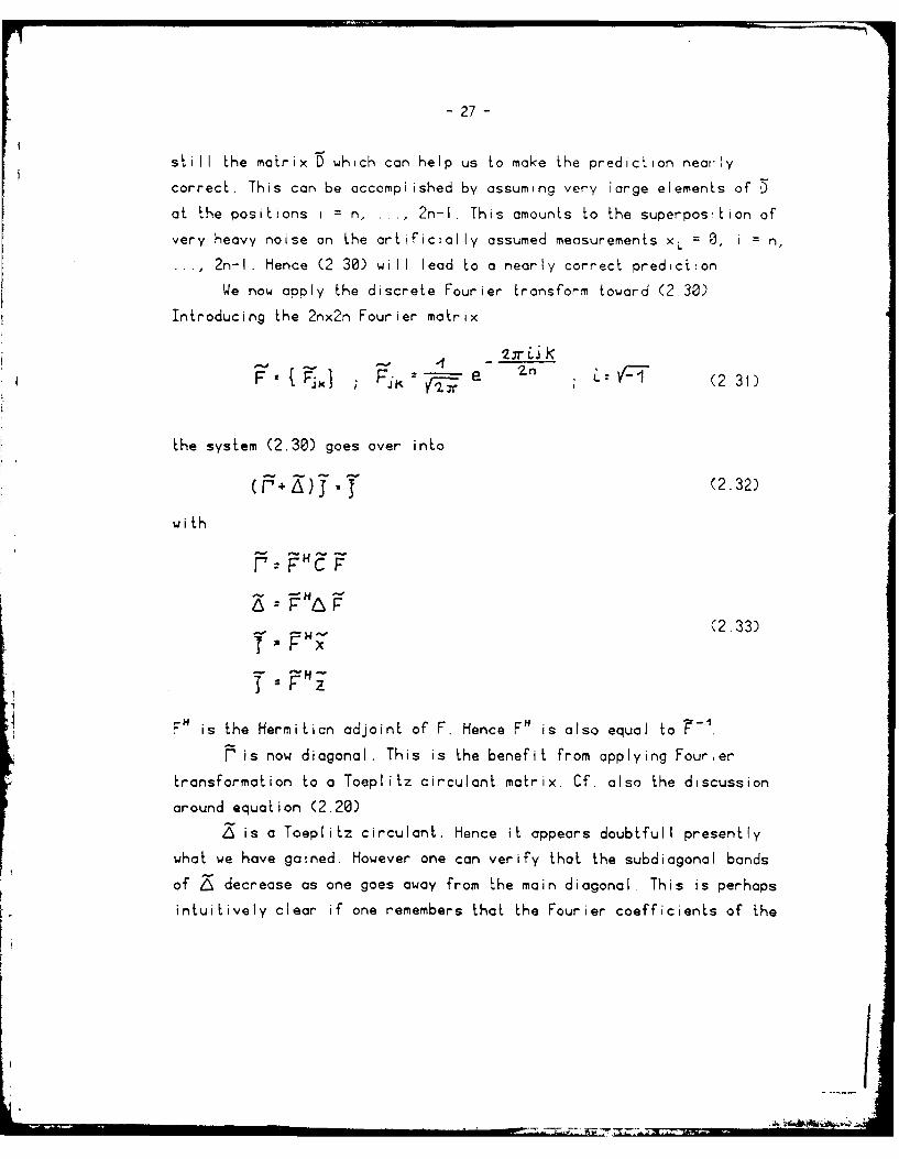
We now apply the discrete Fourier transform toward (2 30)
Introducing the 2nx2n Fourier matrix
F K " e L' VC (2 31)
the system (2.30) goes over into
(.+)j j •(2.32)
with
- - H
(2.33)
F" is the Hermitian adjoint of F. Hence F" is also equal to F-.
is now diagonal. This is the benefit from applying Fourer
transformation to a Toeplitz circulant matrix. Cf. also the discussion
around equation (2.20)
is a Toeplitz circulant. Hence it appears doubtfull presently
what we have gained. However one can verify that the subdiagonal bands
of Z decrease as one goes away from the main diagonal. This is perhapsintuitively clear if one remembers that the Fourier coefficients of the

F1
-28 -
step Function
0 (2 34)
cre given by
I ) (2.35)
2;rn L
The tapering effect of the subdiagonal bands can be made more pronounced
if the transition of small elements of D in CO, n-i] to large ones in
[n, 2n-1] is smoothed out somewhat. This causes "data deemphasis" of xL
near the interval ends.
The next step is to neglect the off diagonal bands of Z up to a
small number m (m = 5 to 10, or so). This truncated banded system
version of the system (2.32) is now solved by Cholesky in O(n) steps.
The rest can be accomplished in O(n log n) steps if the Fast Fourier
technique is employed.
We leave it with this oversimplified picture of the algorithm
which could be extended to the 2-dimensional case. it is interesting to
note that the above mentioned 'data deemphasis effect" is also
encountered in the presentation of the real TASC algorithm.
(4) Shortly before finishing this report, an article by
Bitmead-Anderson (1980) came to my attention. The authors show how an
nxn Toeplitz system can be solved in O(n log n) steps by a doubling
method. The matrix is subjected to some mild restrictions, however
reference is made to other work by Brent et. al. (1980), in which an
O(n log n log n) algorithm is specified which achieves a solution
whenever it exists. It should be noted that no approximations are
involved as they are in the work of TASC. Of course, the question arises
again how large the constant hidden in the *0" symbol really is.

- 29 -
2.7.4. Rauhala's array algebra.
Another way to utilize symmetries was pointed out by Rauhala. Confer
Rauhala (1980) for details and further references Also Snay (1978)
gives an introduction to Rauhala's "array algebra". It is an application
of the concept of multilinear mappings between tensor spaces. Let X, Y,
Z denote 3 vector spaces of not necessary equal dimension. Consider the
space T of tensors:
T = XGYOZ (2.36)
An element of this space is represented by a three-dimensional array
itjd,. T can be viewed as the linear span (set of linear combinations) of
vectorial tensor products xey pz with x EX, yeY, zeZ. The tensor
generated by xeyaz has elements tLjK = xLyz L. Consider three further
vector spaces X', Y', Z' of arbitrary dimensions I', J', K'. Form the
tensor product T' = X' Y' Z'. Let A, B, C be linear operators
X'z Ax-Y' By (2.37)
Z': Cz
Define a linear map T -T' in the following way. Let the image of xe ye z
be Ax@Ay® Az. Extend the domain from the set of tensor products to all
of T by means of linearity. Thus a map Ae Be C from T -T' is obtained.
Suppose, temporarily, that any of the maps A, B, C is invertible. It is
easily proved that
(A"B C Q (2.38)
Here the benefit from array algebra becomes transparent: instead of
inverting a huge matrix of size (IJK)*(IJK), one inverts 3 matrices of

- 30 -
sizes I*I, J*J, K*K.
Assume now I' > I, J' > J, K' > K and consider the leasL squares
problem
t' + V (A (9 E3 5C) t, (2.39)
with LET, 'E T', and vET' denoting the residuals. The 3 least squares
problems
y' v B y (2.40)
Z' I+v,- CZ
are solved by the pseudo-inverses
X •A+,- '
8 #. y' (2.41)
If the rank of A equals the number of its columns, then
A (ArA) iA r (2.42)
and similarly for B+, C'.
Rauhala shows that the pseudo-inverse of As Be C is given by
(A 8 C)+ = A'*80 C +(2.43)
A proof follows easi ly from geometric reasons based on 'range-space' and
"null-space" considerations. We do not give a complete proof here,
because it requires a number of formal definitions. We merely mention
the following facts:
(a) The matrix A maps its domain space one to one onto its range space.
__i
-- - - .4 !

31 -
The orthocomplemenL of the domain space is the null-space
(b) The pseudoinverse maps the range space inversily back onto the
domain space. It maps the orthocomplement of the range space onto zero.
(c) Domain space and range space of A@38&9C are the tensor products of
domain and range spaces of A, B, C. Hence (2 43) is essentially reduced
to (2.38).
Thus the least squares problem (2.39) is solved by
t (A e B+@ C+) t' (2.44)
Let this outline be enough. We just mention that generalization to
tensor products of arbitrarily many factors are immediate. Rauhala will
also forgive that I did not use the most generalized inverses he has
ever invented.
Applications of array algebra are restricted to gridded problems
defined on regions being of the box-type. The grids must be rectangular,
however the spacing between gridlines may vary. The question still
remains how familiar problems of physical geodesy are transformed into
problems of array-algebra. Rauhala states that this cannot be done
without some "cheating a la Gordian knot". The cheating may perhaps be
comparable to that one encountered during the transformation of a
problem formulated for a small spherical rectangle into a translation
invariant problem defined over a plane rectangle.
Let us discuss the computational affort for the case of two vector
spaces X, Y of equal dimension n. The tensor product T = X@Y has
dimension N = n'. The effort to naively solve an N*N system requires
O(N3) = O(n6 ) steps. The effort to invert 2 matrices of nxn is 0(n') =
O(N{). It may be shown that a solution of the system utilizing the
.... ~i.
32 -
decomposilLon A 9 B can also be done in O('JL) sleps. This is
asymptotica;y he same etorl as if a general sparse system resulting
trom a 2-dimensional layout is solved by the nested dissection method.
Confer the discussion in section 2.4, in particular the first of the 2
remarks given at the end of subsection 2.4.
ItI

- 33 -
3 Ou:IHne of the fLnite elemenL approach.
3.1. He-r-lrp-cubic repesentaoion of the field
3.1.1 The four basis funclions for the unit interval
Let
X (, ) (X- M Y)o"(2 >e 6
and define
Too () 2 Y 3x " *1
Y 1 ( ) 'x ( 1 ) 3 2 - 2 (3 .2)
Graphs of these 4 basis functions are shown in figure 3.1
e I
Fig. 3.1 Graphs of basis functions in unit interval
Note that the first subscript in y'rj(x) refers to the location, i.e. x =
0 or x = 1. The second subscript refers to the degree of the derivative
which is equal to unity at that node.
The 4 basis functions solve the following interpolation problem:
34-
g i ven
f(C) . Co f(i) C10
() o C(l) (3,4)
find a cubic po;ynomial inierpoiating these values. The solution :s
(,Y Q~ )(5)L ., 0
We also introduce the derivatives
d.xk
Remark: The coefficients of
3,t, ( - c)(ije x t (3.7)
are stored in the 4-dimensional or.ay PSC(K,I,J,L) during execution of
our computer programs described in chapter 6
3 1.2. Interval of length h
Let
YLJ(x; hh) - h j ; 0_ !5Y h (3.8)
These functions solve the above interpolation problem with data given at
x = 0 and x = I. Again we take derivatives of these : jsis functions:
dj h). .
"~T~ (3 - .9) r.'

- 3S -
Obv i ous I y:
"k Lj be; h h' Yk ( ) (3,10)
3 1 3. Bicubic polynomial in a rectangle with sides a, b
Take
S r, Lyj iY ( xY. y; a,b) - , ), Y-..Lj (y; b)
0 X 6 CLo (3.11)
Note: the first Ewo indices refer to the location, the second pair
refers to the degree of derivatives!
The functions (3.11) solve the following interpolation problem:
Given
f (o,o) C f(o,b) 2CoPoo
f,(0,0) C0001 fY(o.b) C0101 (! (3.12)
foo) • C0040•!f.Yo'o) -OI fw. b
find a bicubic polynomial
3 3f(,,y)- - .s X")s (3.13)
rz0 st0
r:-- 7,0
1 i

- 36 -
interpolat'ng these data The solution is
.Y > - C L..j. Y Y' j*L y wJ bJy
0 0- o (3.14)
0 Y b
3.1.4. Tricubic polynomials in a box with sides a, b, c
The extension to 3 dimensions is obvious: In the interpolation problem
we prescribe the nodal derivatives shown in table 3.1 at i1 e 8 corners
of a box with side-length's a, b, c
j. jyJ, 000 001 010 011 100 101 110 l1l
Deriva~tive f 1K ' f Y- fX f, y fky&
Table 3.1
Numbering of nodal derivatives in 3 dimensions
3.1.5. C continuity across element boundaries.
Consider an n = 1, 2 or 3-dimensional region divided into elements. For
n = 1 the elements are intervals, for n = 2, 3 the elements are
rectangular boxes. For n = 2, 3 we assume that a corner of an element
does not touch the interior of a face (boundary segment, boundary
rectangle) of an adjacent element. Otherwise, the elments need not be
of the same size. Take as an example the partition of a region in R
shown in figure 3.2.

- 37 -
x
Figure 3.2
Sample element partition in 2 dimensions
Assume that the Hermi e nodal values are prescribed at the corners. Then
a function may be interpolated into any of the elements. It is an
n-cubic polynomial there. This function is continuous and has
continuous first derivatives everywhere. Such a function is said to
belong to the class C.
The proof is easy but not entirely obvious. Let us sketch it for
n : 2. Take any segment separating two elements, e. g. the line
segment A-B in figure 3.2. The limits of f(x,y) from the top and bottom
elements are two cubic polynomials f70o(x), fso.,rCx) in x. However such
polynomials are completely determined by the values f(A), f.CA), f(B),
f,(B) which are common to both polynomials. Hence the polynomials must
coincide. The reader may wish to extend the argument to the continuity
of fy across the segment A-B. It becomes transparent why the mixed
derivatives fry are needed at the nodes.

- 38 -
3. .6. Comoound elements.
We will encounter functions which are rough in some areas and smooth in
others. In order to rep-esent them properly and economical y we like to
be able to change the size of tHe elements in a way that is more
flexible than that indicated in figure 3.2. In order to achieve this, we
must sacrifice something, namely the simplicity of the elements. It will
be sufficient to outline the procedure in RL and to consider the"compound element" shown in figure 3.3
6 -7
h4----1-- 5
1= 3
Figure 3.3. Sample of a compound element
The compound element shown has n = 7 nodes. At each node i four nodal
parameters are prescribed. They are fCi), fy(i), f,(i), fY(i). If a
point u is to be interpolated which is situated in the upper quad, we
just take formula (3.13) specified above. Note that also the artificial
node h may be viewed as a node of the upper quad. Its nodal values f(h),
fy(h), f,(h), f.ry(h) are interpolated linearly from these of i = 4 and
5 alone and do not depend on those of i = 6, i = 7. Having nodal
parameters in h, it poses no difficulties to interpolate points in the
lower quads. The interpolation formula for any point x in "he compound
quad may now be written as:
.C.... ( ) .(3 I)

- 3g -
The index i refers now to the nodes, the index j to the nodal
derivative. The basis functions 6Lj (x,y) of the compound quad are
piecewise cubic polynomials. They are composed of cubic polynomials
having as domain Ehe 3 subquads making up the compound quad Note that
the artificic< node h does not enter the interpolation formula. Its
nodal parameters are linear functions of those at the genuine nodes, and
have thus been eliminated. Formula (3.15) holds also for simple quads,
in which case the -j (x,y) are jusL the 1j(x,Y) in a differen
notation.
C1 continuity within the compound quad is obvious. It is further
obvious that C' continuity holds within a region partitioned into simple
and compound quads in a way that any node of a quad is shared by all
neighbouring quads. Figure 3.4 gives an example of such a region.
Figure 3.4. Element partition in R
using simple and compound elements
Of course, alternative shapes of compound elements can be designed.
i4

- 40 -
Figure 3.5 shows some of them.
Figure 3.5
Other examples of compound elements
The idea is always the same: decompose the elements into subelements of
simple, i.e. rectangular shape. Make a choice of nodes which you like to
retain in the final compound element. The nodal parameters at the other
nodes must be linearly expressible in terms of the parameters of the
retained nodes by linear interpolation (not extrapolation!). After
specifying nodal parameters at the retained nodes, interpolation of any
location is done by a formula like (3.15). The basis functions a(x,y)
are obtained by specifying parameter values equal to zero except for one
parameter where a value of I is specified.
3.2. Shape functions.
For presentational purposes it is useful to introduce shape functions.
Consider a region subdivided into finite elements as for example that
one shown in figure 3.4. Label the nodes in some way by i = 1,2,... At
each node, label the nodal parameters (e.g. f, fy, f,,, fy) by i =
1,2,3,4. For each pair (i,j) consider a function SLj(x,y) which has zero
nodal values at all nodes i'i Furthermore, at node i, all nodal
parameters j'+j are also zero. Sjj(x,y) will be nonzero only in
elements adjacent to the node i. This feature is a great advantage
• -.

- 41 -
because precisely the locality of the shape functions Sj (xy) is
responsible for the spasiLty of the normal equations to be derived
later. In a particular element adjacent to node 1, Sj (x,y) of course
coincides with the local functions a(x,y) introduced earlier (cf. equ.
(3.15)). Hence the shape functions SL (x,y) are nothing new. In the
later developments we will mainly deal with their fragments, the element
related j(x,y)'s. However, many interrelationships are more clearly
explained, if the globally defined functions S j(x,y) are used.
3 3. Contribution of the field to the normal equations.
In conventional least squares setups, the normal equations are formed
from observations. Observations will also contribute to the normal
equations in our case. However there will be another contribution. The
harmonicity of the field is not automatically implied by the Hermite
cubic representation. Complete harmonicity is practically incompatible
with this field representation. All that can be done is an approximate
fulfillment of Laplace's equation. This will be achieved by minimizing
the integral over the squared Laplacean of the field. This integral will
give the additional contribution to the normals as announced earlier.
3.3.1. Reasons for excluding the Ritz method.
Our least squares approach may be called an old fashioned one. At least
this is indicated in current treatises on finite elements (cf. Strang;
Fix (1973), pp. 133 to 134). In these treatises, attention is focused on
more modern principles due to Ritz and Trefftz and generalizations of
them published in the lost few decades. Confer Oden (1979). Let us
explain why we do not propose the Ritz principle. (I tried it in
numerical experiments, but it gave poor results!). The Ritz principle
.i, a

- 42 -
is successfully used in the following typical situation
Find a solution of
,A/:V in
(3.15)V q on 8
This is the familiar Dirichiet problem. However not Dirichleticity is
the point. We could have used Neumanns boundary conditions as well, or
even a mixture of both. The decisive point is hat fixed boundary values
are prescribed. The Ritz principle replaces the above problem by a
variational one:
Find a solution of
rc o 18 . P lin . (3 .17)B
subject to
V 9 on 85 (3,18)
The variational formula is slightly more complicated in case of Neumanns
boundary condition, but this is irrelevant presently.
The next step is to replace V in (3.17) by its finite element
representation, i. e. by
V • . -.-i (X.y) (3.19g)
Here V j are the unknown nodal parameters and Sq (x,y) are the known
shape functions. The functional (integral) to be minimized becomes a
quadratic function in the unknowns VLj. The fulfillment of the boundary
conditions V = g at 9B can not be postulated in a strict sense. One has
to be satisfied that V g at certain points of the boundary
II | II

- 43 -
and perhaps also that some derivatives of V and g along the boundary
coincide at these points. The boundary conditions thus yield a linear
set of constraints for the unknowns Vi. Minimization of a quadratic
functional subject to linear side constraints is a standard problem
which leads to the familiar linear normal equations whose solution are
the V .
Consider-a sequence of partitions of B into finite elements such
that the diameter of the largest element goes to zero. It is also
required that the shape of the elements is not too badly distorted as
the diameter tends to zero. In treatises on finite elements it is proved
that under fairly general conditions the finite elment solution
converges to the exact solution of the original problem. The main
advantage of the Ritz method over the more primitive method indicate6
above and to be described in detail below, namely the method of
minimizing
jf(v) 8 (3.20)8
subject to
V at dB (3.21)
is the following one: The Ritz method involves a functional defined in
terms of first derivatives. As a consequence, one may use shape
functions Si (x,y) which are simpler than those required for the other
method. The functional (3.20) is defined in terms of second derivatives.
It is shown in the literature, that our piecewise cubic polynomials,
which are C'continuous across element boundaries, are an admissible set
of trial functions for the least squares problem (3.20, 3.21). However
the Ritz problem can be treated successfully with trial functions which
are only piecewise bilinear and just C0 continuous across element
boundaries. Such functions require only one nodal parameter, namely the

- 44 -
function value f at the node. This holds in 1, 2 or 3 dimensions. Recall
that our C" coninuous shape function require 2' nodal parameters, i.e.
2, 4 or 8 depending on the dimension d. The decrease in number of
parameters o£fers one advantage although it must be balanced against the
need to use smaller elements because of the more primitive nature of the
shape functions. in any case, the computer programs turn out to be much
simpler if bilinear shape functions are used.
But why does the Riiz method not work in our gecdetic environment?
In geodesy the boundary values are the result of measurements.
Measurements are not performed everywhere and they are subject to
observation errors. In some areas the measurements are redundant; e.g.
there may be measurements of V as well as of some components of the
gradient of V. In other areas the measurements may be sparse. There may
also be measurements in the interior of B. The constraints in our
minimization problem become weighted constraints, so to speak. A
problem of balancing Ehe weights arises. The normal equations are the
sum of two contributions, namely that one from the minimization of the
functional, and that one from the observation equations. Symbolically
(p1G1 + p2 G2 )x - r (3.22)
Suppose that the functionca! to be minimized is the Ritz-functional, i.e.
± !9 L VjCL3 (3,23)
If we choose p, large and p, small, then the gradient of V will be made
small at the cost of large residuals al Ehe observations. In the limit
p.-o, we get a constant V. If we choose p, large in comparison to p,
we treat the observation equations practically as constraints. The
minimization procedure will try to match the observations exactly. This
may lead to absurd results in case of redundant observations. Even in

-45-
case of nonredundancy, the resulting function V may be far off from thct
one minimizing the gradient. Hence harmonicity is not ensured. Another
disadvantage is encountered in subsequent error propagation studies. If
one tries to propagate observation errors to some desired quantity, e.g.
a gradient at satellite altitude, the resulting error will reflect the
small p, rather than the large p. This is extremely undesirable,
because the propagated error is then mainly due to a "poorly observed"
gradient rather than to the observation errors. These disadvantages are
to a large extent avoided if we choose the minimizing functional as
j-,f(AV)IOLB (3.24)
From the above discussion it is clear that weights p, should be rather
large in comparison to p7. p1 weighs now the failure of V to be
harmonic, whereas in the earlier case it weighted the failure of V to be
a constant function. There is a lot of harmonic functions which deviate
considerably from a constant function.
If we minimize the functional (3.24), there will be deviations
of AV from the zero function; but these deviations will be small. Hence
the weights p, can be chosen'large in comparison to pL. Errors
propagated after adjustment will therefore mainly reflect the errors due
to the smaller weights p7 which belong to thk observations.
3.3.2. The least squares contribution of the field.
After discussing the reasons for choosing the functional (3.24) for the
purpose to ensure approximate harmonicity, we turn to the technicalities
of calculating the contribution of this functional to the normal
equations. Let us first outline the procedure on hand of the shape
functions SLj(p). As explained earlier, the index i refers to a node
while the index j refers to one of the parameters at this node. The

- 46-
argument p may now be viewea as i, 2 or 3 dimensional In case of
detailed discussions we shall mainly stress the case of 2-dimensional
poiar coordinates, where we write S~j(r, S) instead of S. (p)
The potential is represented as
V V. S.()(2)1. L* (p) (3 25d)LI
Its Laplacean is
AV . 6S (P) (3 26)
If 2-dimensionai polar coordinates are used, the Laplacean is
-1 4 -1LV -- Vrr + t1 It .VYY(.7
In order to have something specific in mind, the reader may imagine the
region 3 in the form of a circular ring In polar coordinates, the ring
becomes a rectangular region. It may be subdivided into simole and
compound elements as shown in figure 3 .6(a) The subdivision shown there
corresponds to a subdivision of the ring which is shown in figure
3.6(b).
t I l t l 1 1 I I I l I 1
Figure 3.6.(a), Partition of a circular ring
represented in polar coordinates

-47-
Figure 3.6.(b). Partition of a circular ring
represented in cartesian coordinates
Such a subdivision may be chosen if the field is anticipated to be more
detailed in the vicinity of the inner boundary. Substituting the
Laplacean (3.27) into the functional (3.24) gives
E :+f( ZVA Lji~)S8p (3.28)

- 48 -
Minim zrng with resoect Lo Lhe Vj leads to Lhe normai equations
2-E 0 nodes (3.29)V .. pcramete-s/node
cr
L j 1 (3.30)
i ... nodes
j ... parameLers/node
Up to a muliiplication of these equations by the weight p1, we get the
contribution of the functional (3.24) to the normal equations. Note that
for a particular equation labeled (i,j), there are only a few nonzero
coefficients, If we write the equations as
9Lj, ;V , V1 0 (3 31)
then
9q; (3.32)
unless the nodes i and i' are "neighbored". Two nodes are neighbored if
there is an element in which both nodes participate. The sparse
structure of the normal equations becomes visible now.
3.4. Detailed instructions for computer imolementation.
If one works with a computer, the above outlined procedure is not
recommended. It is preferable to decompose the total "energy' E

into contributions of the individual elements now denoted Bk.
E:X EkE Ek(3 33)
with
Ek V , r Ljt (p) dS(P) (3,34)
In agreement with the earlier notation Gj(p) for the element-internal
basis functions, this may be written as
E 'f [" jA87,aP1 dP.(p) (3,35)
The summation needs to be extended only over nodes participating in the
element. We may form the 'partial normals" due to the contribution of
element k:
. f [AGj(p)Ce 1,.(P) CLB (P)] V-'j, 0 (3.36)
or
0; IT (3.37)
If there are I nodes participating in the element, and if J is the
number of parameters per node, the above is a symmetric system of IJ
equations.
The normal equations (3.31) for the entire region are obtained by
summing all partial normal equations. The situation is similar to a
network adjustment where partial normals may be formed for subsets

- 5 -
of the measurements; a subset may e.g. be given by a round of directions
Laken ao one saL ion. The partial normals are then combined to yield the
normals of the entire network.
3.4.1. The partial normals of" a simple aucd.
We return to the notation of section 3.1.2. for the basis functions in a
simple quad writing:
V (rV) , -' i(:Cr-r -).yz ,*, (-o; r '' 'o),, (3.38)ijr 41r J r yrv 4,Jr *
The simple quad is assumed Lo exLend over the region
(3.39)
Our nolation appears complicated now. However we are trying to give
detailed instruction for an efficient computer implementation rather
than trying Lo please the casual reader wiLh some slick and polished
notation which suppresses the nasty details.
We form the Laplacean (confer (3.9) on the notation for the
derivaLives of the y's)
rL ,j rj,i ,r 4C rj J zrr J "'YtjY,
" - , .r-r.; r -r.). . ' ; , (r, 1(.,',, "-' ; 1 .rd (3,. ,40')'. S, y,)
l~l l .... I J ..:.:- ., 1| , :,. -• . . ... .. ..I

' - 51 -
Let us abbreviate this for the moment as
3
AV (r. V f Z r'r'r(r)h h .y"" (341)
In order to form the normals (3.36, 3.37) we have to evaluate all
integrals
d T~k,/ r ( r)(,. (r) h' "rctr cLy'~ ~ ~ ~ ~~ - jrJy; ir'4f'jrJ' ' ,J Zrjr TrJ/r ci(~iVt
r.r0 "' ... (3.42)
The coefficients of the partial normals
' 9 rbJ, J ; .'. ' V','J I .O (3.43)*~~i~.'~fi LrjvJ 9 L,'. LJr J'j LrL~yJr'JT.'
are then given by
3 ..E 1K.I -rLYgJr ' : ;r'g'jrJi, (3.44)
It is a great computational advantage that the above integrals decompose
into one-dimensional integrals
iK'2 )K, . (3.45)'
with
rT ' " () Lrr (3.46)
r. r,
.1

- 52 -
It is suff'cienL to outline the furiher procedure on hand of one of
these integrals. Let us take as an example
rr
,r • • ( r- (3.48)
r: ro
We substitute
r + (3.49)
then
I
0
By (3.10) in section 3.1.2. this further equals:
4
. /) Jr;~jr+ i Z ... -r.) (3.51)
The functions ykj,j,(?) are now derivatives of the basis functions for the
unit interval. Confer section 3.1.1., equation (3.6). They are cubic
polynomials whose coefficients are stored in the array PSC(K,I,J,L)
during the computer runs.
According to the outlined rule, we get for any of the integrals
KK
T ZrJr r'!r' (3.52)
an expression of the form
.[r< f Jr r'- c&r(01) " r r(K') * I ( ,3L-JrL jr ( -rQ) dr(3.53
r . .) e( 1
0*'# 4KLj(' ~d 7 KLj- 0C 0 ~( 1 r)

53-
analogous y
I KW -(-
If k)" ,CW"
(3.S4)
0
Thereby
2 -ocJd (3 55)
The following table lists the degrees dr(k), dT(k) and the exponents
e(k)
k dr dy e
1 2 e e2 I 0 -1
3 0 2 -2
Table 3.2
Listing dr(k), d!F(k), eCk), k=1,2,3
All these integrals are extended over weighted products of the basis
functions and their derivatives for the unit interval. These basis
functions are cubic polynomials in one variable. The first and second
derivatives are quadratic and linear polynomials respectively.
Hence all the integrals can be assembled with the help of the
PSC-table and the following integrals over weighted monomials:,t
MS xS(r (0--)x-e xS 0 . $ 6 (356)
0

54-
Summarizing, we obtain the following procedure to evaluate
r "-yJ'rJyl ; Lr' Ly'Jr'Jl
for a simple elemen r. $ r _ rG ; r , S
[HI Evaluate the weighted integrals over monomials according to (3.56)
and tabulate them for g4s46, -34E t41
[27 Us:ng the PSC-Lables, whose coeffiecients are denoted c, rr(Cf.
equation (3.7)!), and the table 3.2 for d(k), e(k), evaluate integrals
over products of normalized basis functions
f W
1''3 3 R K1
2: 2:C r(k) Lrjretr(K)C&r' ~ .Lr'irJ'Pi.e eK eO
-, (3.57)
* 3 KW
2 X - C ,K) ef4'jV'e'M Ce" t .0 if
[3] According to equations (3.53), (3.54) evaluate:
Lrjr .j. ( r,) JrJr'- dr(K) - dro') +11LrJ Lr'r" "Lrlr Lr'jr'
--. .y N- - ( () I K'c' (3.58)
L rl' " ) " "rJry ,J g,
0 6 Lrjr Lr'Jr', L jtf Lytj ,, .
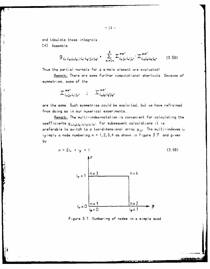
and tabulate these integrals
14] Assemble3 KK I
9 Z' eyj'rjf ;i rjr 48i--' K 3.5 )'k Lrjr 1Jr'
Thus the partial normals for a simple element are evaluated!
Remark: There are some further computational shortcuts. Because of
symmetries, some of the
are the same. Such symmetries could be exploited, but we have refrained
from doing so in our numerical experiments.
Remark: The multi-index-notation is convenient for calculating the
coefficients 9rjiYJjZ'j;-'j'jV For subsequent calculations it is
preferable to switch to a two-dimensional array gL,. The multi-indexes L
Lyimply a node numbering n =1,2,3,4 as shown in figure 3.7 and given
by
n 2ir + iY + 1 (3.60)
r,4
n1 n3 n 4+
Irnr~l n=2
n- n 2 -.iy= 0 i,
Figure 3.7. Numbering of nodes in a simple quad

- 6 -
T he parameter numbering per node has been explained above repeatedly, It
is given by
q2jr +j + I (3.61)
and shown in table 3.3
q Jr "Y Math. symbol
I 0 0 V
2 0 1 V
3 0 Vr
4 I VrT
Table 3.3. Parameter numbering at a node
We adopt an accumulative parameter numbering by
i = 4(n - 1) + q (3.62)
In this way we get a two-dimensional array by:
LL' " LrL~jrJ ; , ~ (3.63)
with
i = 8 ir + 4 i f + 2j , + j f + (3 64I ~ j~ J J~(3.64)
i' = 8ir' + 4i + 2 jr' + j . + i
In this way we get a 16x16 matrix for the present example. There are 16
parameters involved in the simple quad, 4 at each of the 4 nodes. The
numbering groups the parameters for one node together. Table 3.4
explains oil the details once more.

- 57 -
node r i? Jr J) common math ,anguage
1 0 0 0 0 V at lower left corner
2 I 0 0 0 1 V --
3 I 0 0 1 0 Vr r
4 i 0 0 I 1 V. -
5 2 0 1 0 0 V at lower right corner
6 2 0 1 I V, "
7 2 0 1 1 0 V
8 2 0 1 1 1 Vr.19 3 I 0 0 0 V at uppe- lefl corner
10 3 1 0 0 V -
II 3 1 0 1 0 Vr -
12 3 1 0 I 1 Vr. -'-
13 4 1 I 0 0 V at upper right corner
14 4 V -
IS 4 1 I 1 0 Vr -'
16 4 1 I 1 Vr -
Table 3.4. Numbering of nodes and
parameters in a simple quad.
This all is rather irrelevant to the casual reader. It is, however,
essential to the person implementing the method efficiently on a
computer.
Remark: The coefficients gLL' are functions of: r,, r1, It follows
that the coefficients are the same for two quads sharing these
parameters. If all simple quads in a 'layer' r.s r: r, have the same
angular width -y, then the coefficients need to be evaluated only
once!
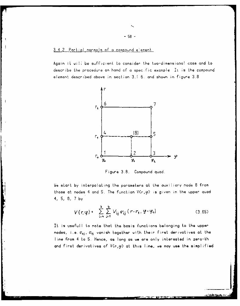
- 58 -
3.4.2. Partial norrmals of a compound element
Again it will be sufficient to consider the two-dimensional case and to
describe the procedure on hand of a spec:fic example It is the compound
element described above in section 3.1.6. and shown in figure 3.8
Ar
r,6 7
r,,
Figure 3.8. Compound quad.
We start by interpolating the parameters at the auxiliary node 8 from
those at nodes 4 and S. The function V(r,97) is given in the upper quad
4, 5, 6, 7 by
V (r ±VLj( r , ) (3.65)
It is usefuli to note that the basis functions belonging to the upper
nodes, i.e. G6j, G% vanish together with their first derivatives at the
line from 4 to 5. Hence, as long as we are only interested in zero-th
and first derivatives of V(r,T) at this line, we may use the simplified

v~ ~~~~ V9 +- , 315
I epresen-!tton
V(rzf)-- X Z V.G (r- , ?-i,) ,o((r-r) 2 )SJ, U U , (3 6)
Using a more exolicil reoresentation we may write
v(r, ) IZJr Jf' O (3.67)
V (Ir.r.r~ (cfY.,j T)
The funchions ';,(x;h) are def ined n section 3.1.2., equation (3.8). loe
are now able to :nteroolate the nodal oarcmeters of the auxi! cry
node 8:
.-.,J ~(3.68)
:or the functions 'rJx) see equations (3 9), (3.10). Switching to the
more condensed noIat or'
J 2 ' r + J I
J (3.69)
.,e Wr e t is releptonshlo as
)(3 70),
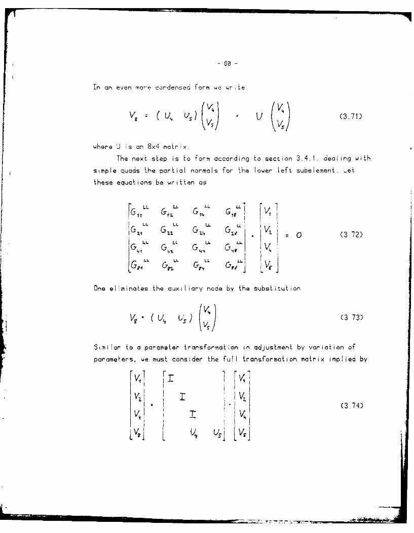
In an even more condensed form we write
, U(3.71)
where U is an 8x4 matrix.
The next step is to form according to section 3.4.1. dealing with
simple quads the partial normals for the lower left subelement. Lei
these equations be written as
G1 ILL LL L L GIU. y[G 5 1 G G VI•G0 0 (3.72)
t.L LL I£.
LL LL ILL
i tG. , 7,fi Vg
One eliminates the auxiliary node by the substitution
v-( % G) (,)Similar to a parameter transformation in adjustment by variation of
poramelers, we must consider the full transformation matrix implied by
V7. V(3.74)
Fr XLv, L4 U S. ud v

-6-
e
v A 7
and iransforrn He aove nor-)cis (3 72), now written as
GV O (3 7 )
according to
A r G AV (3 75)
7he result *s
LL LL LL LLI
i, G Gig7
L0 I f
G- -
11.717
S LL L. LL.
--- L . vs.
L ~
s seen U.a
-- L

- 62 -
LL I. LI.
L .- - O=M 0 , -zUS.
- ". L Lr_ LL T LL344 2 G t. & 1, + 4 lU" &,, U, (378)
-U I. I L- .LL
Ur&:O, LI. u 0 U-G9 L U S r C-nLL S
In a similar way we obtain for ihe lower right quad
GZ 2 G ,, V.
-LR - L - LR - LR
~LA -;ILA -LA -ILAt V (.9
-LK - LA LA -
By a direct application of the simple quad formulas we obtain for the
upper element
I) GI L L/
GCO G5 cS IT VZ v2 vC0 I U LI (3.80)
G6 V G C..' 6 VC
Now the partial normals (3.77), (3.79), (3.80) of the 3 subelements are
added into the normals of the compound quads
iil I I --- . .

-63
GF. 01 G 21 ( G2 2.G 1Z
IC7 7 v V
C-11. G~ VG~ G
An or' th Gm~ ;e 0ii G S~ M ~ Q
LL
where a<~.S , G;; e is cssumea, fone of th odes i orj
does not partcbaKi ' ;sjad or 'J
3. More ger'er-H bcsis ~c ''
This seclior, Tiay se-ve (is ci- o ,'>re For 'Lhe const-uction) of shape
functions which) 'I) -a'o\ e a r eneral araly~ical reDresenitation t han
piecewise ~ ~~oii,(2) are C1 cont ouous, ornd- (3) are
r ompu t at ;or-a i s ezi , Y1 S -' f ; -e t
The ;7--,o~lolo~ r Kor- o hape functions may corneI
from tke d~es."'i o jse frcos Khconlform to the potentials
at-eniuation *n a be~~way. (j-':,-7-- temot ng to replace polynomials
in r b/ pcY,/r-orrials r Inr, F~i e-<'-r,:_' 'k- Thoo~s oortlicularly
attrct i-tor eeMqrITS'c- ow(!) f-)m r,( earth surface it also
Ooer's ri way to roore,;en he'iK't n Wao ori ire exter 'or Df some
sph-ere by a .- ire r-r* - 'er; ite size Th)s csPect will

64-
be treated furiher in the next section.
The computational efficiency of cubic polynomials comes from 2
sources. (1) Such polynomials are easily evaluated, (2) the integrals to
be evaluated in order to form the partial normals of a simple element
decompose into a moderate number of products of integrals over a single
variable. The second feature extends to Lhe basis functions to be
outlined below, the first one extends only partly.
As in section 3.1.1., one starts again with the unit interval. One
introduces functions Yrj(x) such that the j-th derivative of T.xj(x) at
the i-th-interva; end is unity, while all other derivatives at this and
the other interval end vanish. It is important to note that the highest
derivative considered this way need not be ihe same at both interval
ends. To have something specific in mind, consider the basis functions
- , )= 3 - 3 (3
N 2- 3/o(X) !Y -K S + 1 3.3S(x) -3x -x
In this example the second derivative is only modelled at the left end
of the interval, but not at the right end. If the above basis functions

I65-
are changed .o
boir() . x - S + 15x-" - fox ."
(X) ;<.*+ X'4 - 6X'"o (x)) 3 ><I x - 3
I (x 62 3 (3.84)
T (x) 6-3x 15 X - C
X 4 + -LX32. z
then we are dealing with Hermie quintic polynomials. At each node the
zero, first and second derivative can be prescribed.
With the chosen set of basis functions for the unit interval one
can proceed to any finite interval by (cf. section 3.1.2):
~ (3.85)
As in section 3.1.3., two dimensional basis functions ore again obtained
by forming products
iLLJ~yij~)'.~ tq /(3.86)
As indicated by the bar over the last i', there is no need to have the
same type of basis functions for x and for y. For example, one may use
quintics in x and cubics in y.
in order to ensure C' ctnLinuity, the type of basis functions used
in the x-direction should be matched by the element adocenL in the y
direction and vice versa. This poses some problems if one fuses simple
o!ements to compound e!ements However, as long as the basis functions
are polynomials, there is normaolly a way out of any dilemma. In any

66-
case, C~ continuity must be checked very carefully in oil unusual
situat ons.
Remark: If quintics ore used consistently, the resulting function is
even C1 continuous. This may look attractive. Among others, it offers a
way to force the Laplacean to be zero at ai nodes. However, a heavy
price has to be paid in terms of d3 parameters per node (d ... number of
dimensions). For d = 3 there are 27 parameters per node, while in case
of bicubics there are only 8.
The nodal parameters needed in these more general finite eiement
representations follow auiomatically from Lhe one-dimensional basis
functions used. Two dimensions are typical enough for our outline here.
Any node has a degree in the x and y-direc!ion. These two degrees need
not be equal, but they pose restrictions to the basis functions of
adjacent elements. Suppose the degree is 2 in the x-direciion and I in
the y-direction. This holds if quintics in x are multiplied with cubics
in y. Then the 2x3 nodal parameters are automatically given by all
symbolic products of any two elements out of the sets
(3,87)
i.e. they are:
VV v , V (3.88)
The integration procedure outlined in section 3.4.1. and the partial
normals of a simple element must be modified if other basis functions
than cubic polynomials are used. The modifications are, however,
moderate. They amount to a change of the integration formulas for the
required products of one-dimensional basis functions and their
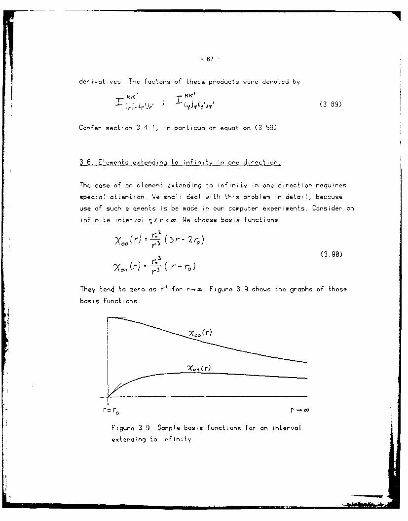
- 67 -
derivatives. The Factors of these products were denoted by
rJrrJr, L j (3 89)
Confer section 3.4.1, in parLicualar equation (3 59).
3.6. Elements extending to infinity in one direction
The case of an element extending to infinity in one direction requires
special attention. '4e shall deal with this problem in detail, because
use oT such elemens is be made in our computer experiments. Consider cn
infinite interva; < r <c. We choose basis functions
(3.90)
They tend to zero as r-' for r-* . Figure 3.9 shows the graphs of these
basis functions.
r= r
Figure 3.9. Sample basis functions for an interval
extending to infinity
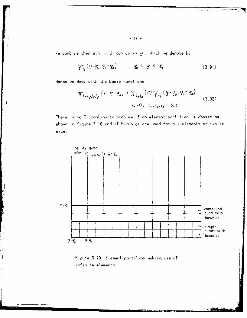
-68-
W4e combine them e.g. with cubics in So, which we denote by
S(Y Y(3.91)
Hence we deal with the basis functions
"ttL~i],j' (,. %) - ;ZM ()Tq f';?''%) (3.92)
0.x , , j y Z'J 0, 1
There is no C' conLinuity problem if an element partiLion is chosen as
shown in figure 3.10 and if bicubics are used for all elements of finite
size.
Infinite quadwith 'L.r-J' r, - 0
-- compoundquad witnbicubics
simptequads with
- bicubics
Figure 3.10. Element partition making use of
infinite elements

- 69 -
Next we outline the integration procedure in detail for the infinite
element. Confer the parallel developments of section 3.4.1 on the
partial normals of a simple quad. The representation of the potential
V(r, y) in a i r, y < y, is
Lr IvJ .i - J 3.3
The index i' is fixed at zero (we retain it only for ease of comparison
with section 3.4.1., equation (3.38)). All other indices run from 0 to
1. The Laplacean is:
tt'rvJrJcr
-L'o (r)$'y . j (3.94)
This equation is abbreviated as
3 ) ( 95)
The principle
(V(r r drcL -in (3.96)
r. GI -To
leads to the partial normals of the infinite quad:
9 Lr jrj; IEvi,,jr.y, Kr'L ,ifj, 0 (3.97)

70-
in analogy Lo section 3A.1., the coefficients follow from the formula:
- I
9 irL' Ji ;Lr K'. I Lrjr ' ( 3.9 8)
The integrals
are unchanged. On the other hand:
p o , . . r)- re(L )r +e((') 1 r
Table 3.3 of section 3.4.?. for the dr, e is sti;l valid. If one writes
the X ,Zr',r in the form
r) C L7+ar~e(3.ioo)) rd Cd .,J r . dr+.
then a compact 3xlx 2x2 table of the coefficients
0 4 dr 7"
CtrLrJ' e Lr 0 (3..01)o _6 j'r 1. 1 3 1
may be stored in the computer. This CHC-Tnb s the counterpart to the
PSC-Table introduced in section 3.1.1. help of the CHC-Toble
one compuLes:
LrJrL~f cJ.-o ~ L~L drW L'rC -0 6 0( 3 .10 2 )
-1r ",-'- d-r0 cr(K)+ e0%)+ e(K'), I
r KC K'e' -

- 71 -
Thereby
Pmeoe 2+ rr(X)+ -+ d dr(O9 + e'- e(K)- e(R')- 1 (3. 03)
3.7. The outer zone.
The infinite outer space of the earth can not be partitioned into
infinitely many elements of finite size. The field is most detailed in
the vicinity of the surface. Hence fairly small elements must be chosen
there. The elements may increase as we go outward. The increase in size
is partly achieved by the natural increase of the surface element rdrdy
or r coscdr dqdA in polar coordinates. To a greater extent it is
achieved by a lumping of elements as discussed in the section on
compound elements. At a certain level the finite element partition may
stop at all. The field is then represented in a spherical shell
(circular ring). It is forced to be (nearly) harmonic there by
minimizing the integral over squared Loplacean. It is now necessary to
ensure in some way that the field in the outer space of the shell is
(1) consistent with the field in the interior of the shell,
(2) approaching zero if the radius tends to zero, and finally
(3) harmonic.
Consistency means in a strict sense, that the outer field is the
analytical continuation of the field within the shell. In a finite
element context this requirement must be somewhat relaxed. Not even
within the shell do we have a strictly analytical field. However, if we
have C4 continuity there, as we do when cubic polynomials are used,
approximate C continuity across the outer boundary of the shell is a
minimum requirement.
There are various ways to deal with the problem of the outer

-72-
field. We shall outline them now.
(1) Choose the radius of the outer shell large enough and force the
field and its first derivatives to be zero there. A large enough radius
means that the size of field and its derivatives must be below the
desired computational accuracy. It must be borne in mind that our field
is actually a disturbing field superimposed upon a reference field.
(2) Partition of the outer space into finitely many elements of infinite
size. Refer to the previous section 3.6 on elements extending to
infinity in one direction.
(3) Use of Greens formula. If potential and (outer) normal derivative
are prescribed at the boundary r, then the potential in the exterior of
r can be represented by Greens 3 "L identity. (See e.g. Heiskanen-Moritz
(1967), equation 1-29').
n ( ) (3.4L V(P) :f{v(Q) 9( n( ) e (P.lSF)
This formula refers to the 3-dimensional case, l(P,O) is the distance
between the reference point P and the point of integration 0. Confer
figure 3.11
n
Figure 3.11. Explains the definition of
outer normal n and distance I

- 73 -
Consider now an element partition within a shell around the earth
surface as shown in figure 3.12.
F Po
Figure 3.12. Fusing the inner and the outer zone
The surface F of integration in equ. (3.i4) is assumed spherical
(circular) and situated slightly inside the outer boundary F,, of the
shell. Greens third identity may now be applied to any node P situated
at the outer boundary denoted r.. Since V(O) and 3v is expressedOnlinearly in terms of the parameters belonging to nodes situated in the
layer between "0 and 1"L, we get linear equations relating V(P) to nodal
parameters of the outer layer (bounded by FT and r). Let V(O) be

-74-
represented as
LL j QJ '-.
Where L represenls the set of nodes participating in the outer layer,
and j runs over the parameters of any node. The Sij(Q) are the shape
functions introduced in section 3.2. We get
) n Sin (3.106)
and
Q 9n -jiV - n el P(Q) (3.107)
The aniounced linear equations are thus obtained:
v(P) - ZZ:C..V. (3.108)ZeL j ij Li
In a similar manner we may even express derivatives of V at P.
Differentiation of Greens formula'poses no problem because P is not
situated at r. Therefore I(P,Q) never becomes zero. For example we may
evalu- e
a v(P)
*2 tVP Ze .V (3.109)
al V(P)~ 9A Ij:fe ~
Representing VCP) and the 'horizontal derivatives' of V at P in this
... :_ .--,. -t-;. i / l i l i
.,77

75 -
way, and doing this for all nodes of I'0, provides us with a set of
linear equations which, together with the normal equations of the
interior of the shell, will ensure a poLt'ntial which is "reasonably
harmonic' outside the earth. A disadvantage of this method, which is
proposed in McDonald-Wexler (1972) and further discussed in Zienkiewicz
et al. (1979), is the need for the evaluation of a number of integrals
which are not ali too simple. The following 3 remarks are considered
important.
Remark i: The reader may wonder why we used only V together with its
horizontal derivatives in the above compatibility equations. The answer
consists of two parts. First we have to point out that the underlying
assumption is that of a tricubic representation of the field. The
"horizontal" nodal parameters V, V9, V ,, Vv.. are, so to speak,
responsible for the variation of V along the surface Fo. Secondly, we
should stress that our finite set of equations substitutes for an
infinite set of equations (3.107) in which P varies all over r. The
variation of P and V(P) along Fo is now logically replaced by the
variation of those parameters in the cubic representation which are
responsible for the behaviour of V(P), for Pera.
Remark 2: The discussion in Remark I also demonstrates an alternative
way in which Greens third identity can be used in order to ensure
compatibility of the field across Fo. Instead of using equations (3.109)
for V9, V,%, V,,., we could just use equation (3.108) for V(P); however, we
must ' it 4 times as often as there are nodes on ro. A way to do this
would te to use (3.108) for the nodes P on Fo and also for the points
halfway between two adjacent nodes. Confer figure 3.13.
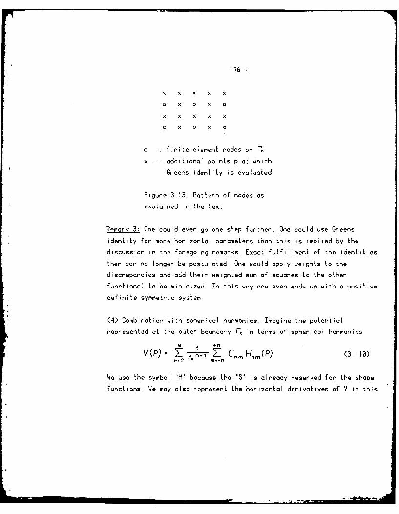
r75
- 76 -
x x x x
o x 0 x 0
x x x x x
o x 0 x 0
o .. finite element nodes on r.
x ... additional points p at which
Greens identity is evaluated
Figure 3.13. Pattern of nodes as
explained in the text
Remark 3: One could even go one step further. One could use Greens
identity for more horizontal parameters than this is implied by the
discussion in the foregoing remarks. Exact fulfillment of the identities
then con no longer be postulated. One would apply weights to the
discrepancies and add their weighted sum of squares to the other
functional to be minimized. In this way one even ends up with a positive
definite symmetric system.
(4) Combination with spherical harmonics. Imagine the potential
represented at the outer boundary ro in terms of spherical harmonics
N +
v1(P)w aZTHn7TZ Cnrm Hm(P) (3.H10)".0 nom-n
We use the symbol "H' because the "S' is already reserved for the shape
functions. We may also represent the horizontal derivatives of V in this

-77-
way
av('P) n __ "_ H, ,(P)Z r. n T Cn nneo P r--n
a V(P) +_ __ n 9.H (P)
Av ) t____n0P m*-n
9% v(P) + n N1) ~ NM(
OA G Z:1- n M dg9
n.0 P M.-n
We form these equations for any node at r,. Imagine that there are just
as many equations as there are coefficients C,,. Then, hopefully, t.he
Cnm Could be evaluated f'rom them. However, we do not propose to do this.
Instead we propose to add equations for the remaining nodal parameters,
i.e.
Z r Cnr,, Hm(P)
i tlsOmr-nv(P) . (n +-1) +") aH M,(P)r , "? Z Cnm o
I n this way, we will ensure that the potential is reasonably harmonic
out~side of" I'. compatible wit.h the f'ield within the shell, and tending to
zero as r-n. .a
Remarks I to 3 given above under (3) apply mutais mutandis to the
present situation.

-78-
3.8. Local data deficiencies.
It may happen that data are abundant and redundant in some areas while
in others they are sparse and deficient. Lack of sufficient data in
local areas can cause rank deficiencies or near singularities of the
normal equations. To illustrate our point, consider Dirichlel's problem
for the exterior of the unit circle:
AV(r ) 0 ; r > I
f (1f)1 (3.113)
V (1) t(o r); r-* 0
Suppose that element partition and distribution of data are as shown in
figure 3.14.
Figure 3.14. Distribution of data leading to
singularities of the normal equations.
Infinite elements are used for the outer zone. It is seen that data are
missing or def, "'mnt in 3 of the 8 intervals at the circurnference of the
unit circle. It follows that a cubic spline function s(y) approximating
• l*

79 -
f(y) in the least squares sense is undetermined. Hence the contribution
of the measurements to the normal equations will have a rank smaller
than in the case of sufficient data. The addition of the contribution of
the field to the normal equations does not remedy the situation. The
field contribution merely serves to ensure (approximate) harmoncity in
the exterior region r > 1. If the boundary data are undetermined in
Dirichlet's problem, the whole field will be undetermined.
Remark: Only to freshmen of adjustment courses it may appear paradoxical
that a rank deficiency occurs when the number of observations exceeds
the number of unknowns. Think of a network which may be rigid and stable
in some areas and poorly determined in others.
There are at least two ways to remedy the rank deficiencies due to
lack of data in some areas. (1) The elements may be chosen larger there.
(2) A third contribution to the normals may be calculated which results
from the square of a certain curvature norm applied to the spline s(')
approximating f(y).
Approach (I) is not too strongly recommended. It may cause a loss
of regularity in the element partition. As a consequence the computer
programs could become more involved.
Approach (2) is related to least squares collocation using
splines. We take the finite element representation of V(l, ')
V1,o) 21j VLSLj (1,) (3.114)L j
The index set L comprises the nodes situated on the circumference of the
unit circle. We take the second derivative
____ cL' .T .Y zv
C 0 1r.L j Ly S0 YLS4
-80-
and consider the integral
V Z (Zv P(CY ay (3.116)0
Here p() is a weight function which con be token p(y) =I. It may also
be taken positive in areas of poor data and zero in areas of sufficienL
data. Taking the variation of (3.116) with respect to V yields, very
much in the some way as outlined in section 3.3.2., a third contribution
to the normals. Sparsity of the normals will not be impaired in any way.
The method readily generalizes to 3 dimensions. The second
derivative with respect to ' may be replaced by the surface Laplacean
thereby.
...I_ I
III.1+---- i + - I III I

- 81 -
4. Estimation of computation time
4.1. Nested dissection and Helmert blocking
Our normal equations can be grouped according to nodes. If d denotes the
dimensions, i.e. d = 1, 2 or 3 and if d-cubics are used, then for each
node there are 2d rows and 2 d columns corresponding to the 2d para-
meters per node. During any step in reordering or reducing the normal
equations the 2 d equations for one node will always be lumped together.
We may view the system as composed of 2dx2d submatrices which could be
called generalized coefficients. Elimination is then carried out using
these generalized coefficients instead of conventional scalars.
In the original normals, two nodes are coupled by nonzero
off-diagonal coefficients if there is a finite element on whose boundary
both nodes are located. Hence the system is sparse. During elimination
the coupling increases due to fill-in. If a node is eliminated all its
neighboring nodes which are not yet eliminated become coupled. The whole
idea of sparse elimination is to renumber the nodes in a way that
fill-in is effectively kept down. We shall use a technique which is acombination of nested dissection and Helmert blocking. The philosophy
behind this procedure was discussed in great detail in Meissl (1980),
sections 3.5.4 -5. Here we shall outline it on hand of a two dimensionalproblem with element partition shown in figure 4.1.
r
Figure 4.1. Element partition serving the outline of
nested dissection in conjunction with Helmert blocking
.4i

-82 -
Mind that we work in the plane polar coordinate system. Hence the region
of figure 4.1 is actually a circular ring, the left and right boundary
line, and the nodes located on them are to be identified. We first
describe the block design in a bottom up fashion. At the first stage, we
consider 8 blocks. Each one is formed out of 2 adjacent squares located
at the bottom level. Such a block looks as shown in an enlarged way in
figure 4.2. We imagine the normals formed for the two simple quads
composing the block, and the normals added. We eliminate from them thenode indicted by a circle in figure 4.2.
Fig. 4.2. First stage block
We call this the inner node of this block. The other nodes (indicated by
crosses) are called junction nodes. We obtain a partially reduced system
of 5 junction nodes.
At the second stage we enlarge the blocks of stage one by adding
two adjacent squares of the next higher layer. The block looks as shown
in figure 4.3. There are still 8 blocks.
Figure 4.3. Second stage block

- 83 -
Each block again shows one inner node. However, this time there are 7
junction nodes. The normal equations for such a node are obtained by
adding the partially reduced normals of stage I and the normals for the
upper squares. After elimination of the inner node, we obtain a
partially reduced system for the 7 junction nodes.
At stage 3 we adjoin to the block of the previous stage one
compound element of the third layer. We obtain 8 blocks as shown in
figure 4.4.
iX
Figure 4.4. Third stage block
The normals are formed by adding the partially reduced normals of stage
2 and the normals for the compound upper quad. The inner node is
eliminated.
At stage 4 we join two adjacent blocks of the previous stage and
eliminate the 4 inner nodes. Confer figure 4.5. The number of blocks is
4 in this stage.

-84-
Figure 4.5. Fourth stage block
At stage 5 we adjoin to the previous block the compound elements of the
upper layer. We obtain blocks as shown in figure 4.6. The scale of this
figure is now the some as that of figure 4.1. The number of blocks is
still 4.
Figure 4.6. Fifth stage block
At stage 6 we lump two adjacent blocks of stage S. See figure 4.7.

-85-
Figure 4.7. Sixth stage block
At stage 7 we do a similar thing; confer figure 4.8
IXFigure 4.8. Seventh stage block
Recall-that the modes of the two outer boundaries are actually
identical. In the final and 8-th stage we eliminate just these nodes.
See figure 4.9

- 86 -
V
Figure 4.9. Eights stage block
The Helmert blocking procedure is, as we feel, best understood, if it is
described in the above bottom up fashion. In order to analyse various
block designs, however, in particular block design for 3-dimensional
problems, we prefer a top down fashion, which we briefly outline for the
above example.
At stage 8 we slice the spherical ring by a dissecting line. Inner
nodes are those located at this line. The dissecting line is indicated
by an arrow in figure 4.9.
At stage 7 we dissect the block again (arrow in figure 4.8) and we
repeat this at stage 6. Inner nodes are still those nodes located at the
dissecting line. At stage 5 the dissecting line is horizontal (figure
4.6). Here we discover the rule which will be general enough for all our
element partitions:
Rule for identifyi.n inner nodes and iunction nodes: Inner nodes
are those nodes located at the dissecting line which have not been inner
nodes before. (In 3 dimensions we deal with dissecting surfaces rather
than lines). Junction nodes are inner nodes of the next higher stage
together with junction nodes of the next higher stage located in the
block under consideration.
The dissecting lines of the stages 1-4 are easily recognized from
figures 4.2 through 4.5 (arrows).

-87 -
4.2. Global solution.
We consider a finite element partition which allows to model the details
of the field near the surface with about the same resolution as a
conventional surface layer or collocat:on solution based on lox i block
averages of gravity anomalies.
The dimension is 3 and we use tricubics. This implies that there
are 4 parameters available at each node which are responsible for the
horizontal variat ion of V in the vicinity of this node. Hence the
element size near the surface must be chosen as 2'x 20. Mind that the
number of blocks is the same as the number of nodes. Consequently there
are 4 parameters available to model the horizontal variation of V in a
block. It follows that the averages over gravity anomalies in the four
lox 10 subblocks can be matched exactly. Our surface of computation will
be a sphere. It may be imagined as a sphere slightly below the earths
surface. The computational effort of solving the normals is unaffecied
by the use of a more complicated reference surface. Only the formation
of the normals takes longer. Asymptotically, i.e. for very large
systems, formation is negligible in comparison to solution. By assuming
a concentric sphere with an appropriately larger radius we obtain a
sphericai shell. Our element partition refers to this shell. It is
specified in figure 4.10(a),(b) and in tables 4.1 to 4.3.
zone block size Number of Number of
from to latit. fongit. blocks along blocks in
(degr. latit.) (degrees) a parallel zone
0 72 2 2 180 6480
72 84 2 6 60 360
84 90 6 18 20 60
Table 4.1 Element partition in first (bottom)
layer as well as in second layer

-88-
Figure 4.iO(o)
Elemnent parti'lon for goba solution

AD-AO,# 164 OHIO0 STATE UNIV COLWUS DEPT OF BOETIC SCIENCI F/0 G/bTHE USE OF FINITE ELEMENTS IN PHIYSICAL *EODEST.(U)APR as P MEISb. F19628-79-C-0075
UNCLASSIFIED. 055.31,3 AF*L.TR-SI-0I11 ML
-, EmhEEEEEmhEIEEEEEmhEEEE oE

-89-
Figure 4.10(b). Element partition for global solution.
Detailed view of area near the pole
The tables apply to the northern hemisphere. The partition for the
southern hemisphere follows by symmetry. In the bottom layer there are
13800 blocks over the whole sphere. Note that the area of the sphere
divided by the area of a 20x 2' equatorial block gives about 10300.
Let us pause for a moment and reflect on the computational effort
associated with a surface layer solution based on 20x20 blocks. (Recall
that only 10xl0 blocks would be about equivalent to our finite element
treatment). We are dealing with a system of 13800 unknowns. The unknowns
ore the densities for the blocks. To solve a linear symmetric system of
iunknowns by a direct elimination method requires about
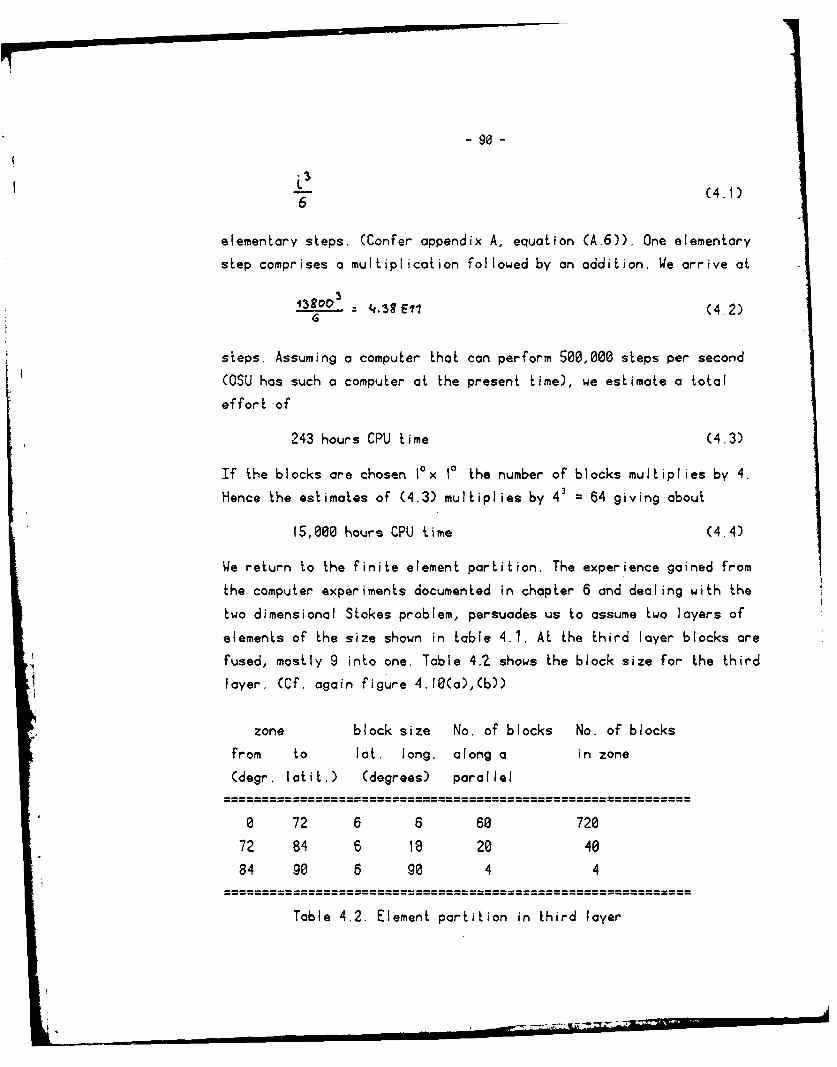
- 90 -
1. (4.1)6
elementary steps. (Confer appendix A, equation (A.6)). One elementary
step comprises a multiplication followed by an addition. We arrive at
'.38 Ell (4 2)
steps. Assuming a computer that can perform 500,000 steps per second
(OSU has such a computer at the present time), we estimate a total
effort of
243 hours CPU time (4.3)
If the blocks are chosen lax 10 the number of blocks multiplies by 4.
Hence the estimates of (4.3) multiplies by 43 = 64 giving about
15,000 hours CPU time (4.4)
We return to the finite element partition. The experience gained from
the computer experiments documented in chapter 6 and dealing with the
two dimensional Stokes problem, persuades us to assume two layers of
elements of the size shown in table 4.1. At the third layer blocks are
fused, mostly 9 into one. Table 4.2 shows the block size for the third
layer. (Cf. again figure 4.10(a),(b))
zone block size No. of blocks No. of blocks
from to lot. long. along a in zone
(degr. latit.) (degrees) parallel
0 72 6 6 60 720
72 84 6 18 20 40
84 90 6 90 4 4
Table 4.2. Element partition in third layer

- g1 -
At the fourth layer the same partition is used. At the fifth layer we
fuse again, table 4.3 shows how.
zone block size No. of blocks No. of blocks
from to lot. long. along a in zone
(degr. lalit.) (degrees) parallel
0 72 18 18 20 80
72 84 12 90 4 4
84 90 6 360 1 1
Table 4.3. Element partition in fourth (upper) layer
Within the main zone -72" to +72' the basic building block is a 180 x 180
configuration. We call it a 6tN'stage block. The meaning of this name
will become clear later on. The face of such a 6,h-stage block shows a
pattern of nodes as depicted in figure 4.11. We count 46 nodes on this
face, and 8 along a side line.
In the following, we assume a blocking strategy for the formation
and solution of the normals as outlined in the previous section. Thenormals result from the contribution of the field and of the
observations. Confer section 3.3. It is important that the observations
are local. Any observation must only involve points situated in one and
the same element. The contribution of the field in the outer zone is
assumed to be taken into account by finite elements of infinite size.
Confer section 3.6. The partition is that one shown for the last inner
layer in table 4.3.

-92-
Figure 4.11. PaLLern of' node oL a IaLerol
face of a stag. 6-block

- 93 -
(10) (9) (8) (7)
(6) 5 1
Figr 4.72. Blocking scheome for globai golion nope e
comol
03 (2
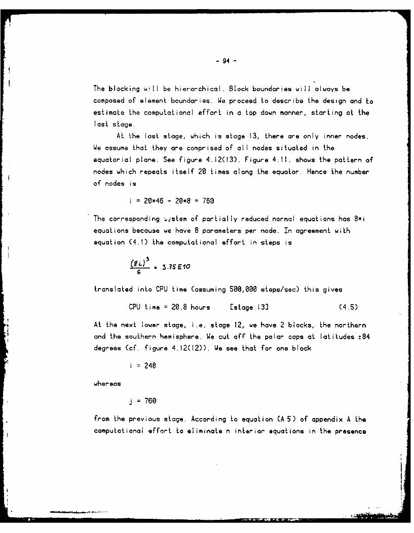
- 94 -
The blocking will be hierarchical. Block boundaries will always be
composed of element boundaries. We proceed to describe the design and to
estimate the computational effort in a top down manner, starting at the
last stage.
At ihe last stage, which is stage 13, there are only inner nodes.
We assume that they are comprised of all nodes situated in the
equatorial plane. See figure 4.12(13). Figure 4.11. shows the pattern of
nodes which repeats itself 20 times along the equator. Hence the number
of nodes is
i = 20*46 - 20*8 = 760
The corresponding .fsLem of partially reduced normal equations has 8*i
equations because we have 8 parameters per node. In agreement with
equation (4.1) the computational effort in steps is
3.75 E10
translated into CPU time (assuming 500,000 steps/sec) this gives
CPU time = 20.8 hours [stage 133 (4.5)
At the next lower stage, i.e. stage 12, we have 2 blocks, the northern
and the southern hemisphere. We cut off the polar caps at latitudes ±84
degrees (cf. figure 4.12(12)). We see that for one block
i = 248
whereas
j = 760
from the previous stage. According to equation (A 5) of appendix A the
computational effort to eliminate n interior equations in the presence

WM
- 95 -
of m junction equations is
n m )(4.6)6 2
In our case n = 248*8, m = 760*8. Hence the effort in steps is
[-! + . j( J] (4.7)
Translated into computer time, and multiplied by the number of blocks
(=2), this gives
CPU time = 55.5 hours [stage 123 (4.8)
We proceed to the next lower stage, i.e. stage It. We are still dealing
with 2 blocks. Each block is divided into two parts by the Greenwich
meridian. Keeping figure 4.t2(1) in mind we count in one block
i = 8*46 + 2*34 - 12*8 = 340
interior nodes (along the dividing meridian) and
j = 760 + 248 = 1008
junction nodes (at 00, ±840). The CPU for both blocks is estimatedat
CPU time = 135.1 hours [stage 111 (4.9)
At the next lower stage, which is stage 10, we are dealing with 4
identical blocks. Cf. figure 4.12(10). Each one comprises a quarter of
the sphere. We subdivide each block by the central meridian. For one
such block we have
i = 4*46 + 34 - 6*8 = 170
j = 10*46 + 2*(4*46 + 34) + 2*70 - 22*8 = 860

- 96 -
We obtain a total CPU for this stage as
CPU time = 86.6 hours [stage 10J (4.19)
At the 9-th stage we have 8 blocks corresponding Lo the 8 octants. We
cut off the region near the pole by dissecting along the surface
= t720. See figure 4.12(g). We have
i = 5*46 - 6*8 = 182
j = 13*46 + 2*34 + 70 - !6*8 = 608
we obtain
CPU time 101.8 hours [stage 93 (4.10a)
From now on we describe the details only for the area bounded by the
latitudes t720. The portions enclosed by latitudes 72oy , 840
-7o f -840 wi II be treated summarily later on.
At stage 8 we cut fhe octant (truncated at = ±720) into 5 slices
as shown in figure 4.12(8). The meridians are eliminated in a sequence
implied by the figure. The effort results from the following table 4.4
No. i j CPU
I 144 684 93.9
2 144 456 45.9
3 144 532 60.1
4 144 456 45.9
Table 4.4. Computational effort
for the 4 phases of stage 8
Summing for this stage we obtain
CPU time = 245.8 hours Estage 83 (4.11)
- 97 -
At stage 7 we have 40 blocks in the shape of slices as shown in figure
4.12(7). Each slice is split into 4 blocks. The elimination of the
dividing lines proceeds in a sequence as shown in figure 4.12(7). The
effort results from the following table 4.5
No. i j CPU
1 30 380 26.6
2 30 228 10.13 30 228 10.1
Table 4.5. Computational effort
for the 3 phases of stage 7
We obtain for this stage a
CPU time 46.8 hours [stage 7] (4.12)
At stage 6 we are dealing with 160 180x180 blocks. We split one block
into 2 parts by a spherical surface between the 3rd and 4th layer.
Confer figure 4.12(6). We have for one block
i=4
j = 4*46 - 4*8 = 152
The resulting CPU for all 160 blocks is
CPU time = 2.2 hours [stage 6) (4.13)
We ignore the upper blocks in the sequel. Their contribution is
marginal.
At stage 5 the number of essential-blocks is still 160. We
decompose anyone of them into 3 subblocks of size 6 degrees by 18
degrees. Cf. figure 4.12(5). There are two phases, and each of them has
i= 26

- 98 -
whereas
= 4*38 - 4*5 + 2 = 134
= 2*38 + 2*27 - 4*5 = 110
The effort is
CPU time = 21.8 hours [stage 5] (4.14)
At stage 4 we have 488 blocks. (Figure 4.12(4)). Each one is subdivided
into three 6°x 60 blocks. Again there are 2 phases:
i =6
j = 2*27 * 2*16 - 4*5 = 66
j = 2*38 + 2*16 - 4*5 = 88
CPU time = 5.4 hours [stage 4] (4.15)
At stage 3 the number of blocks is 144e. (Figure 4.12(3)). We eliminate
the 4 nodes at the lower face of the upper subblock. Consequently we
have for one block:
i =4
I = 4*16 - 4*5 = 44
CPU time= 1.7 hours Cstage 3] (4.16)
The upper portion cut off in this way does not have any interior nodes
and is therefore ignored.
At stage 2 (see figure 4.12(2)) we eliminate the 4 nodes situated
below those eliminated in the previous stage:
i=4
j = 4*12 - 4*3 + 4 = 40
CPU time = 1.5 hours Estage 2] (4.17)
At the first stage the 4 inner nodes at the bottom of each of the 1440
blocks are eliminated (see figure 4.12()!)
......

- 99 -
S= 4
j = 4*8 - 4*2 + 4 = 28
CPU time = 0.7 hours [stage 1] (4 :8)
We now return to the chips of the octants cut off in stage 9. They are
located between t72 and t84 degrees of latitudes. Their structure is
best seen from figure 4.10(b). Table 4.6 summarizes the elimination
stages necessary to decompose these blocks.
Stage Dissecting surface i j No. blocks CPU
8' spherical between 4 304 8 0.4
3-rd and 4-th layerI
7' A = const., 16 264 8 1.4
producing 5 slices
16 132 8 0.4
18 178 8 0.6
16 132 8 0.4
6' y= t780 6 81 40 0.2
5' as in stage 32) 4 44 80 0.14' as in stage 2 4 40 80 0.13' as in stage 1 4 28 80 0.
=3.6
1) Upper portion ignored in the sequel
2) blocks of stage S' and 3 are identical. They are
60 x6 blocks involving layers 1,2,3.
Table 4.6. Complementary stages for regions at high latitudes
Hence we obtain
_____________________________________________ --

CPU time = 3.6 hours [stages 8' to 3']
The total CPU is obtained by summing over all stages
Tolai CPU t!me = 729 hours (4.ig)
Remark: We have been somewhat wastefui by al owing many elements of
small width (6 degrees longitude) at latitudes 9- ±84 One could at the
lower layers imagine an intermediate ring of elements between 84 and 86
degrees latiudes whereby the longiLudina; width would be 18 degrees.
This would probably reduce the total CPU time to about 600 hours.
in any case it turns out that the problem is not managable on a
computer do'ng only half a million steps per second. However there are
faster computers. The ILLIAC IV is described in Avila et.al. (1978) as a
machine ihat has 64 processors, each of a speed comparable to that one
assumed above. All processors execute the same instruction at a time,
but each one operates on a separate data stream. Data can be exchanged
between processors (a subset of the processors can be disabled under
program control). Such a machine appears to be well suited to cut down
the CPU time by a factor which may approach 64. The elimination
procedure outlined above can be viewed as a procedure eliminating nodes,
whereby each node contributes 8 parameters to the system. We may thus
view our linear system as one having as many unknowns as there are
nodes, however each unknown represents acLua ly a subvector of 8
elements. From the viewpoint of eliminating nodes, an elementary
operation is thus a multiplication of two 8x8 matrices followed by an
addition. There should be a way to organize these operations such that
all 64 processors of the ILLIAC IV are busy all the time.
It appears, after all, that a global solution is feasible if one
of the worlds best computers is available. However, I consider it
doubtful that such a computational adventure will be undertaken in the
next future. Fortunately enough there is another bonus available in
physical geodesy, as well as in other disciplines, which allows us to
calculate a detailed and good solution in a local area of interest
7 . -'V

without being forced to calculate such a detai led solution everywhere.
The effect which we are going to exploit, and which has been exploited
a lot in the past, is called "the remote zone effect". It is called, by
the way, 'St. Venant's" principle in elasticity theory.
4.3. The remote zone effect.
There is not much need to elaborate on it at length. Everybody knows
that the details of the field in one area hove little correlation with
the details in remote areas. Put it in other words, if the field is
changed in an area e.g. by changing the mass distribution in this area,
the high frequent features in remote areas remain practically unchanged.
In applications of Stokes and Vening Meinesz formulas this effect is
utilized in a way, that detoi led data are only processed in a fairly
small area around the point of interest. The remote zone effect can also
be exploited in conjunction with other methods, e.g. the surface layer
method, the collocation method and, of course, the finite element
method. We shall consider two configurations. The first one is a strip
in which a detailed geoid is sought. The second one is a local region,
which for simplicity will be taken as rectangularly shaped.
4.4. Detailed solution in a strip.
Consider a partition at ground level as shown in figure 4.13(a). Assume
that this pattern extends around the globe, and that the central line
corresponds to the equator. The size of the smallest squares is assumed
to be 2'x 20. The partitioning of the space outside the surface
(assumed spherical) is demonstrated in fig. 4.13(b). The size of the
elements increases as we go away from the surface. The outer zone is
assumed to be partitioned into specially designed elements which share
two more nodes at the north- and south-pale. See also fig. 4.14.

- 1t2 -
F4. tgl o
9I
- -4-F
-igure-------. t-o- -
ection - as idi
- -4-------------4--
A - - -- - - - A'
Figure 4 .13(:a). Part.ition a0 . ground level o f strrip
Figure 4.13(b). Part.ition of vert.ical cross
section AA' as indicat.ed in f'igure 4.12(a).

Figure 4.14. Elemnent partition for solution
in equatorial strip
The potential at the two nodes at north- and south-pole will be assumed
to be known. Only a very much smoothed version of the potential is
needed there, Hance these nodes will not contribute to the
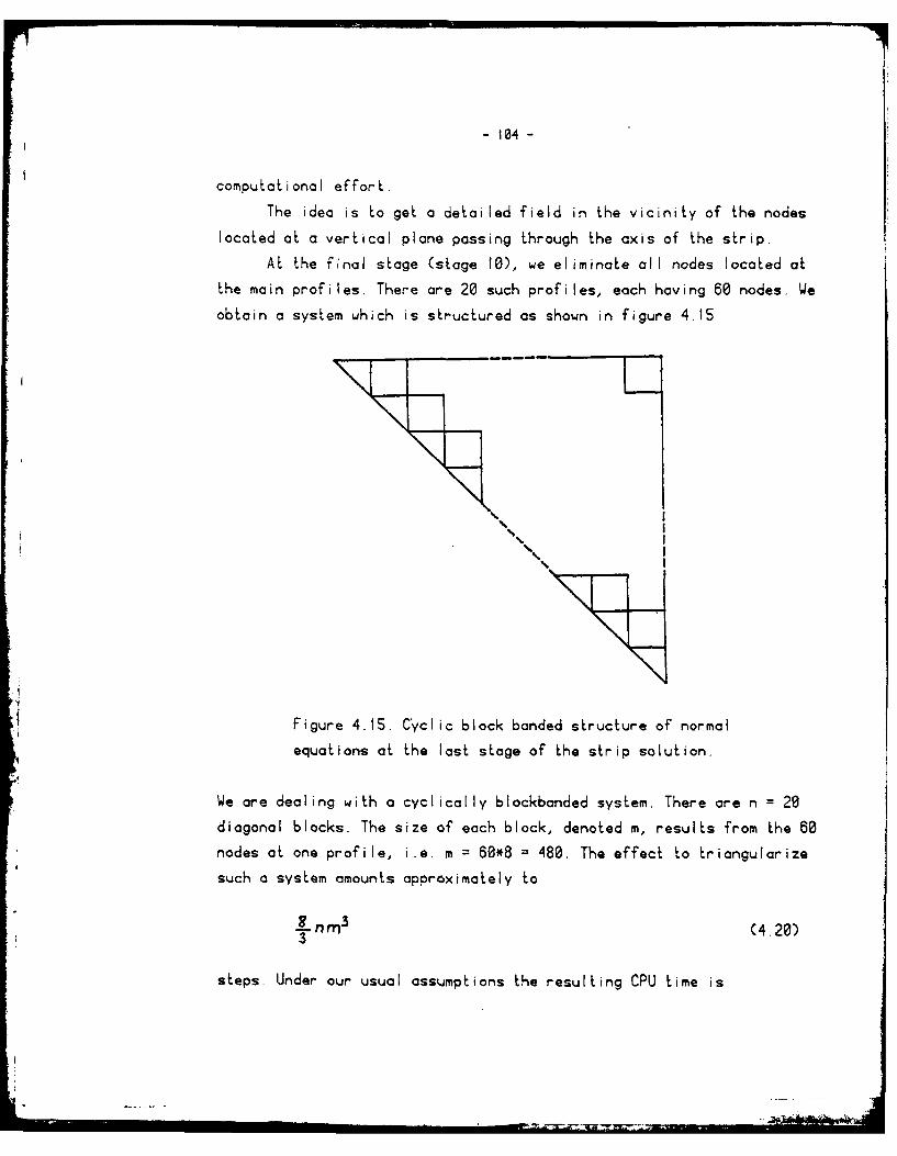
- 104 -
computational effort.
The idea is to get a detailed field in the vicinity of the nodes
located at a vertical plane passing through the axis of the strip.
At the final stage (stage 10), we eliminate all nodes located at
the main profiles. There are 20 such profiles, each having 60 nodes. We
obtain a system which is structured as shown in figure 4.15
Figure 415. Cyclic block banded structure of normal
equations at the last stage of the strip solution.
We are dealing with a cyclically blockbanded system. There are n = 20
diagonal blocks. The size of each block, denoted m, results from the 60
nodes at one profile, i.e. m = 60*8 = 480. The effect to triangularize
such a system amounts approximately to
.-n m3 (4.20)
steps. Under our usual assumptions the resulting CPU time is
-- m ... .... , ......... _. ~Z - , . . .. " : .. ..
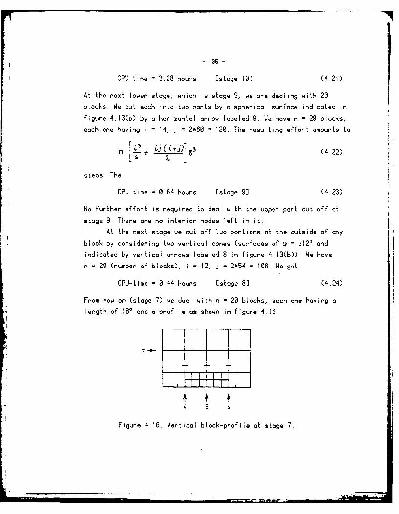
- lOS -
CPU Lime = 3.28 hours [stage 10] (4.21)
AL the next lower stage, which is stage 9, we are dealing with 20
blocks. We cut each into two parts by a spherical surface indicated in
figure 4.13(b) by a horizontal arrow labeled 9. We have n = 20 blocks,
each one having i = 14, j = 2*60 = 120. The resulting effort amounts to
n L *J) 3 (4.22)
steps. The
CPU time = 0.64 hours Estage 9] (4.23)
No further effort is required to deal with the upper part cut off at
stage 9. There are no interior nodes left in it.
At the next stage we cut off two portions at the outside of any
block by considering two vertical cones (surfaces of = ±12 ° and
indicated by vertical arrows labeled 8 in figure 4.13(b)). We have
n = 20 (number of blocks), i = 12, j = 2*54 = 108. We get
CPU-time = 0.44 hours [stage 8] (4.24)
From now on (stage 7) we deal with n = 20 blocks, each one having a
length of 180 and a profile as shown in figure 4.16
7--0
4 1
Figure 4.16. Vertical block-profile at stage 7.

-106-
We cut off the upper level by a spherical surface indicated by an arrow
labeled 7 in figure 4.16. We have i= 6, j=2*40 + 2*11 =102. Hence
CPU-time 0.19 hours [stage 7] (4.25)
At stage 6 we cut each of the 20 blocks into 3 parts by 2 planes
vertical to the ground level and the axis. There are two steps, each one
having i = 26. The number of junction nodes is j =79 and .j = 70
respectively.
CPU-time = 1.14 hours [stage 6) (4.26)
At stage 5 we are dealing with n = 60 blocks. We bisect by a vertical
axial plane. See the vertical arrow marked 5 in figure 4.16. We count
i= 6, j=2*35 = 70. The number of blocks is n = 60. Hence
CPU time = 0.27 hours [stage 5) (4.26a)
At stage 4 we remove the lateral portion of each of the 120 blocks. See
the arrows labeled 4 in figure 4.16. WJe find i = 6, j = 2*20 + 6 = 46
CPU time =0.25 hours Cstage 4) (4.27)
The profile of a stage 3 block looks as shown in figure 4.17. The depth
of such a block is 6 degrees of longitude. Hence the horizontal cross
section is square shaped. Ve are still dealing with 120 blocks. At each
of the subsequent 3 stages we cut by a spherical surface. See the arrows
labeled 3,2,1 in figure 4.17.
2 -
Figure 4.17. Vertical block-profile at stage 3

- 107 -
AL stage 3 we have: i 4, j = 4*14 - 4*4 40
CPU-Lime = 0.12 hours [stage 3] (4.28)
AL stage 2 we have: i = 4, j = 4*12 - 4*3 = 36
CPU-time = 0.10 hours Cstage 2] (4.29)
AL stage I we have: i = 4, j = 4*8 - 4*3 = 20
CPU-time = 0.03 hours [stage 13 (4.30)
The total CPU Lime is
Total CPU-Lime = 6.46 hours (4.31)
4.5. Rectangular renion.
Consider a region of interesL covering an area of 32°x 640 (the
conterminous United States are contained in such a region). Augment this
region by adding layers of succesively larger elements to account for
the remote zone effect. The element design at ground level is seen from
figure 4.18. Note that the element size at surface level is now lox 1° .
The vertical design is based on 4 layers of elements. The lower
two layers follow the pattern of figure 4.18. At the third layer we fuse
4 blocks into one, and we do the same at the fourth layer. The basic
building block of our element design is thus a block, which we call
5-sLage block. The element partition at one of its four vertical faces
is shown in figure 4.19 (a). There are 25 nodes on a face and 7 nodes at
a vertical edge. The corresponding blocks for the augmented zones are
shown in figure 4.19 (b), (c).

1010
F igure 4.18. Element partition at
ground level of rectangular region
(a) (b) (C)
Figure 4.19. Element partition at vertical block
faces in solution for rectangular region.

109- leg -
At the final stage (stage 12) we imagine a bisecting vertical plane
passing through the central meridian. See the arrow labeled 12 in figure
4.18. We count
= 8*25 - 7*7 + 2*13 - 2*5 + 2*6 - 2*3 173
Hence
CPU time = 0.25 hours [stage 12] (4.32)
At stage 11 we split along the central parallel. Accordingly
i= 8*25 - 8*7 + 1*13 - 5 + 1*6 - 3 = 155
whereas
j = 173
There a two blocks
CPU time = 2.85 hours Estage fl] (4.33)
At stage 10 we have 4 blocks. Any of them is split into two subblocks
along its central meridian:
i = 4*25 - 4*7 + 1*13 - 1*5 + 1*6 - 1*3 = 83
j = 12*25 - 11*7 + 2*8 + 2*3 = 245
CPU time 3.90 hours [stage 10] (4.34)
At stage 9 we have 8 blocks. We split by parallels. There are 2 types of
blocks. For four blocks we have
i = 4*25 - 5*7 = 65
j = 12*25 - 11*7 + 2*8 + 2*3 = 245
CPU time = 2.86 hours
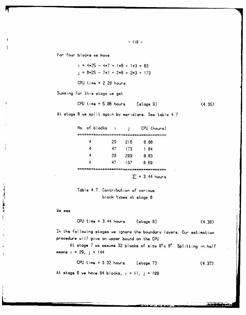
-Ho-
For four blocks we have
i= 4*25 - 4*7 +1*8 + 1*3 = 83
j= 8*25 - 7*7 + 2*8 + 2*3 = M7
CPU time = 2.20 hours
Summing for this stage we get
CPU time = 5.06 hours [stage 9] (4.35)
At stage 8 we split again by meridians. See table 4.7
No. of' blocks i j CPU (hours)
4 29 216 0.88
4 47 173 1.044 29 209 0.83
4 47 137 0.69
=3.44 hours
Table 4.7. Contribution of various
block types at stage 8
We see
CPU time = 3.44 hours [stage 8) (4.36)
In the following stages we ignore the boundary layers. Our estimation
procedure will give an upper bound on the CPU.
At stage 7 we assume 32 blocks of size 80'x 80. Splitting in~ halfmeans i =29, j =144
CPU time 3.32 hours [stage 7] (4.37)
At stage 6 we have 64 blocks, i =11, j = 108
CPU time = 1.29 hours [stage 6] (4.38)
At stage 5 we have 128 blocks of size 40x 40. We remove the upper layer:
i 1, j = 72
CPU time = 0.10 hours [stage 53 (4.39)
At stage 4 we have still 128 blocks. We bisect by a vertical plane: i
10, j 4*21 - 4*5 + I = 65
CPU Lime = 0.89 hours [stage 43 (4.40)
At stage 3 we bisect the 256 blocks once more: i = 3,
= 2*16 + 2*8 = 48
CPU time = 0.27 hours [stage 33 (4.41)
Now we have 512 blocks of size 20x 0We remove the upper half: i = 1,S:4*8 = 32
CPU time = 0.08 hours [stage 2] (4.42)
At stage I we remove the two lowest nodes at the central axis of a
block: i = 2, j = 4*9-4*3 + I = 25
CPU time = 0.10 hours [stage 1] (4.43)
Summing up we obtain:
Total CPU time = 21.55 hours (4.44)
This is still quite forge. On the other hand, if one owns a computer,
such computation times are not unrealistic.
4.6. Further effort to cut down the computation time.
Examining the above models, in particular the global one and the
rectangular one, one realizes that most of the computation time is spent
Ma~j
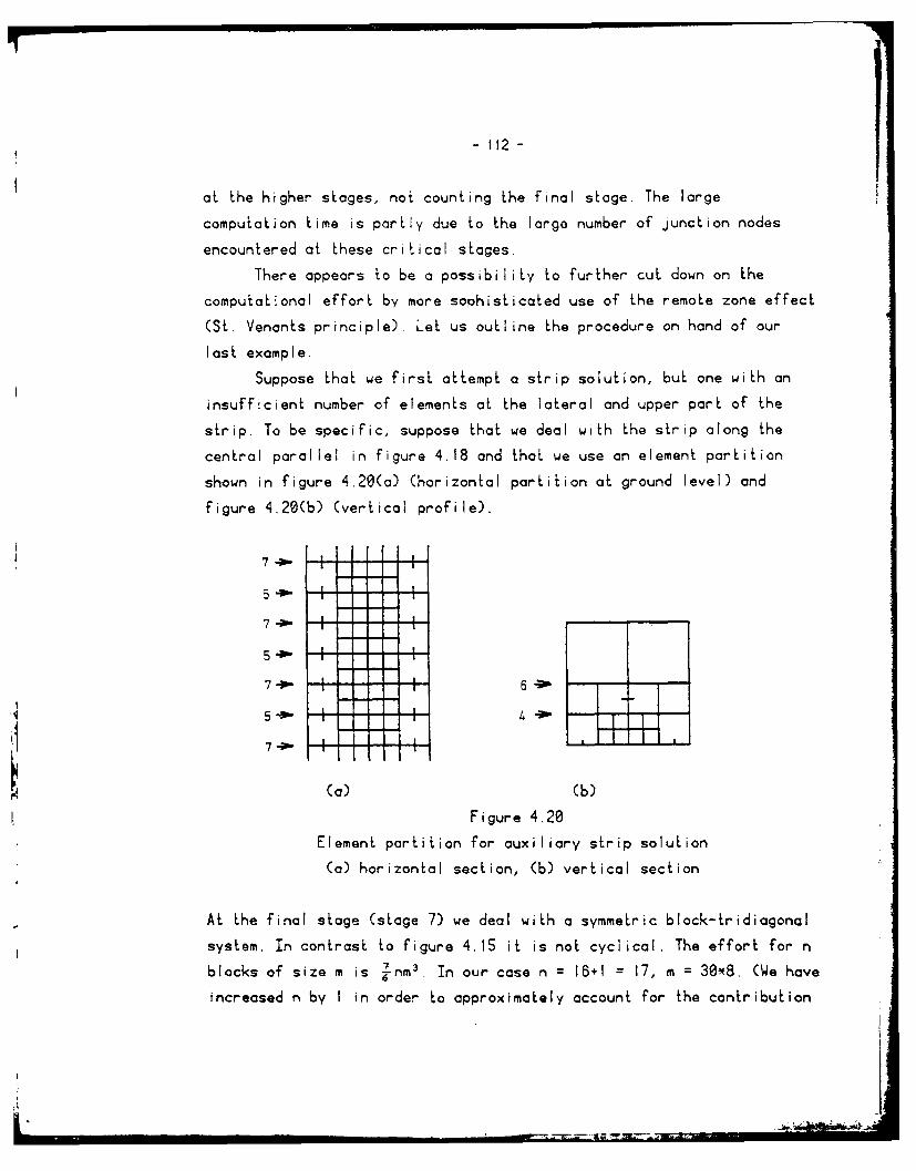
- 112 -
at the higher stages, not counting the final stage. The large
computation time is partly due to the large number of junction nodes
encountered at these critical stages.
There appears to be a possibility to further cut down on the
computational effort by more sophisticated use of the remote zone effect
(St. Venants principle). Let us outline the procedure on hand of our
last example.
Suppose that we first attempt a strip solution, but one with an
insufficient number of elements at the lateral and upper part of the
strip. To be specific, suppose that we deal with the strip along the
central parallel in figure 4.18 and that we use an element partition
shown in figure 4.20(a) (horizontal partition at ground level) and
figure 4.20(b) (vertical profile).
7..
-P,- -4 I,71
(a) (b)
Figure 4.20
Element partition for auxiliary strip solution
(a) horizontal section, (b) vertical section
At the final stage (stage 7) we deal with a symmetric block-tridiagonal
system. In contrast to figure 4.15 it is not cyclical. The effort for n
blocks of size m is -nm . In our case n = 16+1 = 17, m = 30*8. (We have
increased n by I in order to approximately account for the contribution

-113-
of the boundary elements), Hence
CPU time = 0.15 hours [stage 7] (4.45)
At sicge 6 we cut off the upper blocks: i = 5, j 60, number of blocks= 16
CPU time = 0.04 hours [stage 6] (4.46)
At stage S we cut into halfes by a vertical plane orthogonal to the
axis: i = 22, j = 2*27 + S = 59, number of blocks = 16
CPU time = 0.25 hours [stage 5] (4.17)
At stage 4 we remove the upper blocks: i = 5, j = 54, number of blocks =
32
CPU Lime = 0.07 hours [stage 4] (4.48)
At stade 3 we remove the lateral elements. We have i= 4, j = 2*21 + 5 -
47, number of blocks = 32
CPU time = 0.04 hours [stage 3] (4.49)
We have 32 blocks shaped as in figure 4.21
/
Figure 4.21. Block at stage 2
We cut into halfes by a vertical plane along the axis: i = 2, j = 39,
number of blocks = 32
CPU time 0.01 hours [stage 2] (4.50)
At stage I we remove the two remaining inner nodes: i = 2, j = 25,

- 114 -
number of blocks = 64
CPU time = 0.01 hours [stage I] (4.51)
Hence
Total CPU-time = 0.57 hours (4.52)
It is seen that such a profile can be calculated in about 0.5 hours.
Profiles in meridional directon require about 0.25 hours.
Figure 4.22. Partition of rectangular region after
auxiliary profile solutions hove been calculated
We calculate 3 long and 7 small profiles as shown in figure 4.22. The
CPU time = 3.72 hours
The potential and its nodal derivatives are not thought to be known
precisely at the axial plane after a profile calculation. However the

i15 -
high frequent portion is thought to be known with good accuracy. This
means that in the further treatment of the rectangular region we may go
along with a smaller number of junction nodes at the vertical planes
along profiles. The number of junction nodes along a profile follows
from figure 4.19 (b). Considering this reduced number, the computation
time for the various stages of section 4.5 is now reduced as shown in
table 4.8.
Stage i j No. CPU
12 (final) 91 1 0.04
I1 75 91 2 0.36
t0 43 123 4 0.51
9 27 123 4 0.29
43 91 4 0.31
8 I1 96 4 0.06
27 91 4 0.17
11 107 4 0.08
27 75 4 0.12
7 29 64 32 0.82
6 11 66 64 0.51
5 (estimated from earlier values) < 0 10
4 10 50 128 0.55
3 (estimated from earlier values) < 0.27
2 < 0.08
I < 0.10
< 4.37
Table 4.8. Reduced computational effort for the solution in a
rectangular region after the calculation of auxiliary profiles

We obtain a
Total CPU time =8.09 hours
Facit: there is always a way to improve on~ a previous estimation. We
feel that also the 700 hours for the global model could be cut by the
above procedure to a fraction of 1/3 or better.
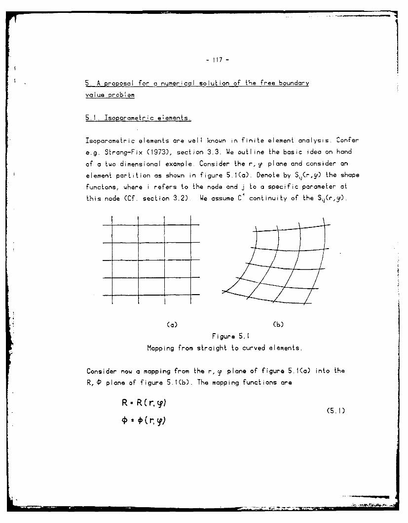
- 117 -
S. A proposal for a numerical solution of the free boundary
value oroblem
5.I. Isoparametric elements.
Isoparametric elements are well known in finite element analysis. Confer
e.g. Strang-Fix (1973), section 3.3. We outline the basic idea on hand
of a two dimensional example. Consider the r, T plane and consider an
element partition as shown in figure 5.1(a). Denote by SV(r,cp) the shape
funclons, where i refers to the node and j to a specific parameter at
this node (Cf. section 3.2). We assume C continuity of the SI(r,y).
(a) (b)
Figure 5.1
Mapping from straight to curved elements.
Consider now a mapping from the r, y plane of figure S.A(a) into the
R, ' plane of figure 5.1(b). The mapping functions are
R~ R (r, ()(R.,)*((S.I)

- 118 -
The elements get distorted thereby. The distortions shall be locally
smooth. The mapping functions shall be C' continuous. In fact, we
represent them in terms of finitely many porameters by using exactly the
shape functions S(r, )'
R: = _R S (r.)! (5.2)
LjU
It is now the R,4 plane of figure 5.l(b) where our problem in terms of a
differential equation of the field and in terms of observations on this
field is posed. The r,y plane of figure 5.1(a) serves only an auxiliary
purpose during the calculations.
There is Laplace's equation for the field:
AV(R,O) -;• ' R OR + R- "910.t
And there are point measurements involving V(R, ) and its derivatives.
In order to have something specific in mind, assume that the image
of the unit circle r = 1 in the r, T plane is the (finite element
approximation of the) level surface of the reference potential in the
R,O plane. Assume that point gravity anomalies are prescribed at certain
locations k = 1,2-.... K which are the images of r = I, F = y,. Let i;
= V be the normal to the level surface in the R,4 plane. Then the
following equations hold (V ... disturbing potential, ... normal
gravity):
A9 VA k R R (1
0, N , )(.4

fig -
Our next problem is to represent the potential in the Rj plane in terms
of finitely many parameters. Here, a deliberate detour is taken. One
starts representing the image of V in the r,' plane in terms of the
shape functions:
iLj 9 tjL
The representation of V(R, ) is then obtained by means of the inverse
functions
r r t-(.() ,R-'(R,(D)
R. ) • (R. ) (56)
Fortunately enough, the inverse functions will never be used expl icitely
during the numerical calculations. We obtain
V (R, 0) V . - S' £ ( r (R.'(), .(P)) (57)
LjU i
Remark: The fact that the same share functions S are used in order to
represent the transformation and the potential is responsible for the
name "isoparametric elements".
We now outline the calculation of the field contribution to the
normals. Inserting the above representation of V(RO) into the Laplacean
(5,3), we obtain
V (R'0) V(5.8)~LJ
The following manipulations serve to circumvent the explicit use of
r(R,), 9(R,0) during the subsequent calculations. Let us take the term
-S.9

as an example. It holds that
a'sz ?- ~r (S.5 10)
+ )Sci. ally~
ol (9 -1 R
The functions
r o r (SLI
dont require any further treatment because the Sjj are simple
expressions in r, S, e.g. bicubic polynomials which ore differentiated
as shown in section 3.1. Of course, after differentiation the
substitution r = r(R,O),y = So(R,¢) has to be imagined but this
substitution will readily be undone during a subsequent change of
variables in the integrals. Only thf derivatives of r, S with respect to
R cause trouble. One forms the Jacabian matrix of partials
__ a __
d r(r, ) (5. 2)
i,_.-_ I: • ,c u~m ...... nrn

- 121 -
One inverts this matrix:
obtaining in this way the first order partials
0 ;"" "(5.14)
whereby the substitution r = r(R,C), y= S(R,P) must be imagined, but is
not done explicitely. Denote 1emporariiy
9 R e(r.,) ar
Then
'r gc)e(r T) 9r ) e(r, ,) sp
(5. 16)ole (r,}er @~~, no__r_ 3(r 9')Or
similarly:
~- r-"
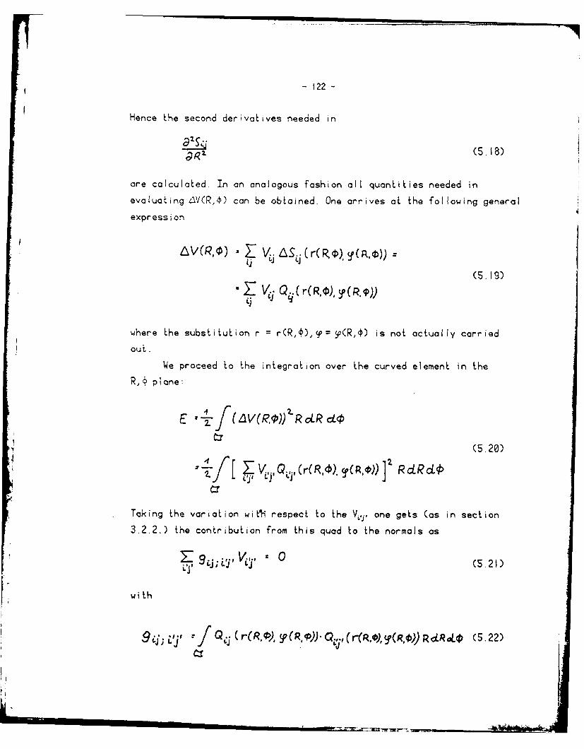
- 122 -
Hence the second derivatives needed in
OR (5. 18)
are calculated In an analogous fashion all quantities needed in
evaluating V(R, ) can be obtained. One arrives at the following general
expression
•~~V LS.. C r( R,), y(A,O)),jj Li
(5.19g)
,j
where the substitution r = r(R,c),9= P(R,0) is not actually carried
out.
We proceed to the integration over the curved element in the
R,. plane:
E .4fo(~P) LR ctP
(5.2S)
Taking the variation witi respect to the Vuj, one gets (as in section
3.2.2.) the contribution from this quad to the normals as
j 9 .,v..., "j; 0 (5.21)
with
9i; Lj ' " f Q (r(R. ), .)Q,.,(r(.R,),Y(R, R,::RoL (5.22)

- 123 -
Now comes the announced transformation of parameters of the r,y plane.
The domain is mapped onto the uncurved rectangle in the r, T plane.
Det[J(r,q;)] is the Jacobian determinant of this transformation.
J4J;LJ r Q ( (r) R(r )'Dot3( q)Jdroy (5,23)
Remark: Although the functions 0 (r,T), R(rg) readily split into sums
of products of terms F(r)G(9), the Jacobian DeLEJ(r,F)] does not. Hence
the integration procedure is not easily carried out. Numerical
integration may be necessary.
Let us also elaborate on the contribution of the measurements, in our
special case, the gravity anomalies. First we need a representation of
the vector v'-, i.e. the normal to the level surface
R, R (1,Cy)(5.24)
We may view this as a oarameter representation of the surface. In the
orthonormal system
ea• , e e (5.25)R 9R,
the vector tangent to the level surface (curve) has the representation
2a
1(5.26)L OT
I
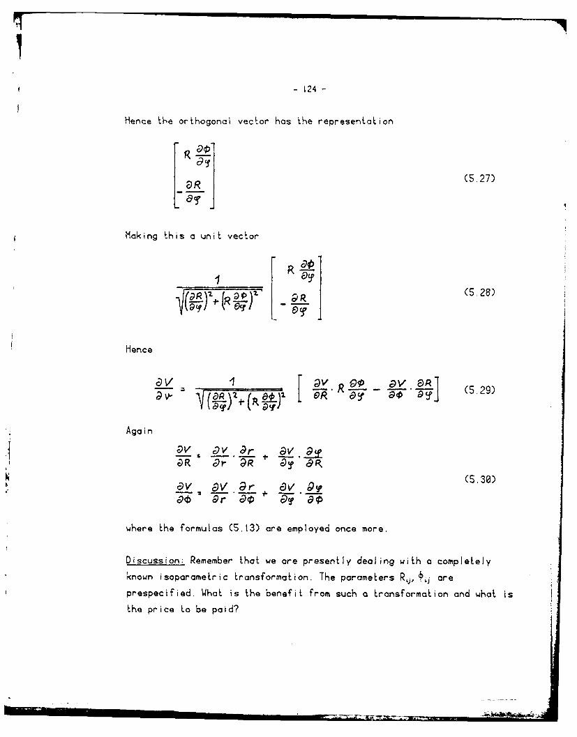
- 124 -
Hence the orthogonal vector has the representation
aR (5.27)
L ac
Making this a unit vector
LR RpV (5.28)6T) *
Hence
av ' r"R , -1 - (5.29)
Again
a_v = V cv r _ _&R 9- . c~ qT
v c9v oR r c9_.V R. (5.30)9V 6aV ar _) _9
where the formulas (5.13) are employed once more.
Discussion: Remember that we are presently dealing with a completely
known isoporametric transformation. The parameters R, ji ore
prespecified. What is the benefit from such a transformation and what is
the price to be paid?

- 125 -
An isoporametric transformation opens the way to exotically shaped
reference surfaces. The resulting normal equations ore still as soarse
as those for the spherical (or ellipsoidal) reference surface Hence the
solution of the normals require no additional effort. A price has to be
paid when the normals are formed. The integration procedure is more
costly with respect to programming effort and computation time. On the
other hand, the solution of the normals is asymptotically more time
consuming than the formation. If N is the No. of elements at ground
level, then the formation of normals is an effort of cN where on the
solution is an effort c5 N. Here cF and c, are (nearly) constants.
Recall, by the way, that a solution by means of surface layer elements
or collocation requires cN'! It is seen that isoparametric elements
affect the constant factor c, but not cs .
5.2. Approaching the free boundary value problem of physical geodesy
Isoparametric elements as outlined in the previous section open a door
to approach the fundamental problem of physical geodesy in a more direct
way than this has been done thus far. Our subsequent presentation will
be expository. Detailed formulas will be given elsewhere.
The fundamental problem of physical geodesy is the simultaneous
determination of the earths figure and potential from measurements of
the 3-dimensional gravity vector at the earths surface. The historical
approach to this problem seemingly has been done under the motto: 'First
linearize everything in sight and then think about formulating a
meaningful problem". As already proposed in Meissl (1971) we prefer to
formulate a problem and then to linearize it. However, we assume that
the unknown surface of the earth is smooth. This means that the terrain
has been smoothed and that the gravity measurements have been corrected
accordingly.

- 126 -
Assume that a sphere of radius r. situated in r, y, A space is the
pre-image of the earths surface under a certain unknown transformation
R - (-
A. A( weA)
Assume that the measurements g, g, ... of the 3 dimensional gravity
vector are taken at locations identified by their coordinates r, =
ro , cp , A, in r, y , A space. The vectors g,, themselves are considered to
be represented in a rectangular equatorial system. Assume further, that
the earths rotation is known so that the rotational part of the
potential can be taken into account by a known reference potential U,
while the unknown disturbing potential V can be assumed harmonic.
The transformation from r, 9, A space to R, , A space is now set
up according to equations (5.2) in the previous section as
Ot~Z jr £.l, R) (5.32)
A A 4iA) r
The R, Aj are assumed known for all nodes i except those situated
at the earths surface. We define the index set L in a way that ieL
identifies precisely these nodes. Thus Ri, kq, Aq are assumed unknownfor ie L. The remaining coefficients Rq, 4 , AJ, i L are known and can
be chosen according to computational convenience. For example they can
establish a transition from spherical surfaces r = const to ellipsoidal
surfaces in the R, 0, A space.

- 127 -
Next the contribution of the field to the normal equations is
considered. One forms the energy integral
E A f V(0,,A)]R cos0cLRcLc-A (5.33)
It is now extended over the entire exterior space in R, t, A space
Unknown quantities in this integral are not only the nodal values Vg but
also Ri, q., A., ie L. Hence variation of E must be performed with
respect to all these quantities. Thereby the usual decomposition of the
domain into the individual elements is employed, and a transformation of
the element integrals back to r, ?, , space can be done just as outlined
in the previous section. The resulting normal equations are linear with
respect to VLj but nonlinear with respect to R j, ij, Azj, i L. They are
of the following form
The equations are still sparse if considered as linear equations in VL.
However sparseness also extends to the nonlinear equations in the
following sense. Any nonzero coefficient gj;L , is related to one or more
elements coupling the nodes i and i'. Hence g j; , will only involve such
transformation parameters R, ,P, A,,, keL which belong to these common
elements. In other words, if the nonlinear normal equations are
linearized, then the resulting equations will have the same sparsity
pattern as the equations of the earlier chapters. The only difference is
that all nodes ieL will have additional parameters R zp.tj, Aj.
The contribution to the normals from the assumed gravity
measurements does not pose much difficulty. The observation equations

- 128 -
cre ot the following type
a)y I 1K'9K
U is the reference potential, V the disturbing potential. The equations
are again linecr in V , but non inear in Rj, k, / ;ie L The reference
potential U also gives a contribution due to the unknown location of the
measurements, i.e. due to the unknowns R , , .i e L. The residuals
r), ,r ,', r, ' are weighted and nonlinear normals are formed. They will
show an analogous sparsity pattern after iinearization.
The normals of field and measurements are added and solved by
Newtons met-od, This method requires precisely that linearization which
we were talking about above.
We shall conclude this outline of an intended research project
with the following
Remark: It is not considered that the use of three-dimensional gravity
measurements is very meaningful in the geodetic boundary value problem
unless additional information on horizontal position is available, Such
information comes either from ground control networks or from space
observations. Hence one should attempt to either incorporate this
information (without destroying the sparsity pattern) or to remove the
horizontal degrees of freedom in the unknown mapping from r, , space
to R, 0, A space.

129 -
6. Computer experiments for 2-dimensional problems
6 I. Purpose and scope
The computer experiments to be described in this chapter were designed
to find an answer to the following specific questions.
1) Should the finite element- approach be based on the Ritz-, or the
Trefftz-, or on the least squares principle. As we have pointed out in
section 3.3.1. the least squares principle was found to perform best in
the presence of noisy and redundant data.
2) Are cubic polynomials sufficiently accurate, or should quintic poly-
nomiais be used? The question is perhaps posed in an overly simplified
way. One can always account for the lower degree of the cubics by
choosing a smaller element partition. Hence the question should be asked
as follows. Does it pay off to replace the choice of cubics and an
adequate element partition by the use of quih-tics and an element
partition having appropriately larger elements? Quintics look attractive
because they are C' continuous. One can even enforce Lhe Laplacean to
vanish at the nodes. Nevertheless it was found that the use of cubics is
preferable.
3) Can the aLtenuation-with-altitude-effect of the potential be
exploited in a way that the size of the elements increases with altitude
fast enough to ensure that the total number of nodes is bounded by a
constant times the number of nodes at the surface. The answer is
affirmative.
4) What is the best way to represent the field in the remote outer space
of the earth? It is believed that specially designed elements of
inifinite size together with appropriately chosen local shape functions

-130 -
(dIfferenL from cubic polynomials) are the best choice. Confer section
3.6.
5) What is the best ratio between weights applied to the field
contribution to the normals and those applied to the contribution from
the geodetic observations?
6) Is there a way to combine in one calculat ion surface data with
satellite derived spherical harmonics?
Due to the large CPU-times predicted for 3-dimensional calculations it
was decided to conduct the experiments in 2 dimensions. Stoke's probiem
for the unit circle was solved by means of finite elements, and for a
set of artificially generated data. Our version of Stoke's problem is
formulated as follows. Find a potential V(r,c?) in the outer space of the
unit circle such that
(4 • 0i -lo (6.1)
( ) L 0 r > 1 (6.2)
(3) V(r i 2V f(c9 ; r 1 (6.3)t r"
It is seen that we have eliminated the logarithmic part of the
potential. V may be viewed as a disturbing potential. The reference
potential U may absorb the logarithmic part. The function f(S) must be
free of 'circular harmonics' of the zero-th and first degree. (I.e. its
Fourier series must start with terms in cos 2S, sin 2y).
Remark: Obviously the stated problem is most easily solved by means of
circular harmonics, i.e. by Fourier-analysis. Representing f(C) as
f(CC) C n(c(c?+ n * sinnsp) (6.3a)nfsZ.

- 131 -
the solution is obtained as
V(y): T1 ( O.ncos n3 1 bnsin n?) (6.3b)n.2.
with
an - bn n (6.3c)
n-I n-
The above continuous version (6.1-3) of Stoke's problem is replaced by a
discrete one. First, the continuous data f(T) are replaced by f(,) for
discrete arguments T, Secondly, the potential V(r,So) is replaced by a
finite element representation
. Lj S j(r.) (6.4)
Confer sections 3.2. and 3.3.1, in particular equation (3.19). The
element partition is shown in principle in figures 3.6(a)-(b) of section
3.3.2. In all experiments conducted thus far, the arguments y were
assumed equally spaced.
The outer zone was represented in two ways, namely by a 'circular
harmonics* representation of comparatively low degree (cf. section 3.7,
method labeled (4)), and alternatively by elements of infinite size as
outlined in section 3.6.
The data f( ) were generated from an "assumed potential' of the
form
VSS (r cf) FZ "n {cL, cos ng *b1.sin n }22 (6.5)
af'- b,'"
- 132 -
The coefficients oL,, (3 were randomly generated in the interval C-0.5,
+0.5]. The maximal degree N, and the damping exponent d were varied.
The choice d = I corresponds to Kaula's rule of the thumb. (Equal degree
variances of the radial derivative for a wide range 2 n < NMAX).
Remark: Note that no measurement noise was assumed to be superimposed
upon the data calculated from the assumed potential
The procedure described in chapter 3 and section 4.1 yielded the
potential at the nodes of the chosen element partition together with the
nodal derivatives. This 'calculated potential' was compared with the
assumed potential (6.5). Statistics of the deviations were calculated
and tabulated. The calculations were carried out on the OSU-Computer
Amdahl 470 V/6-II. In a few cases, a post-analysis of the OSU results
was done on a desk-top computer WANG 2200 VP. The potential was then
interpolated into the interior of the finite elements in order to verify
that the approximation was also good there. Also a few orbits of passive
masspoints were numerically integrated for the assumed potential and,
alternatively, for the calculated potential. In both cases a circular
symmetric reference potential of the log r type was superimposed.
6.2. Parameters distingujishing the experiments.
In this section we give a detailed description of the input parameters
characterizing one particular experiment.
IDEGR degree of polynomials in elements of finite size:
3 ... bicubic polynomials
5 ... biquintic polynomials

-133-
ISWINF a switch distinguishing the represenitation of the field in
the remote outer zone r > rour
I ... circular harmonics
2 ... elements of infinite size
NLAYER number of successive layers of elements in the circular
ring I < r < rour
ITYPECI), I I, ..... NLAYER type of elements in layer number I
I ... simple quads
2 ... compound quads
NELEM(1) number of elements in layer number I (the lowermost)
layer
HFCT a factor governing the thickness of the various layers
and also responsible for the size of rour. Cf. the following
remark.
Remark: From the input parameters NLAYER, ITYPE(I). I = I, ... , NLAYER,
NELEM(I), HFCT the element partition was calculated by the following set
of formulas:
NELEM(I) = NELEM(I-I)/ITYPE(I-I); I = 2, ..., NLAYER (6.6)
DELPHI(I) = 2*r/NELEM(I); I = 1, ..., NLAYER (6.7)
RADIUSI) =I
RADIUSCI) = RADIUS(I-I)*(l + DELPHI(I)*HFCT)
I = 2, ... , NALYER+I (6.8)

- 134 -
Thereby we have denoted
NELEM(I) number of elements in layer I
DELPHI(I) angular width of elements in layer I
RADIUS(I) inner radius of layer I
outer radius of layer I-I
I = 1 ..., NLAYER
RADIUS(NLAYER+I) = ror outer radius of last layer outer radius
of the circular ring partitiored into elements of finite
size.
4e now continue to describe the input parameters.
NPOTC largest degree of circular harmonics in assumed potential
(denoted NMAW in equation (6.5))
DAMP damping factor in the assumed potential (denoted d in
equation (6,5))
NPINST this parameter governs the number of locations at which
data (gravity anomalies) were calculated from the
assumed potential. Remember that the locations are equally
spaced. NPINST is the number of locaLions in an interval
of size DELPHI(I), i.e. in a boundary segment of a
lowermost finite element at r = 1. The data are
arranged there as shown in figure 6.I. It is seen that
the interval ends corresponding to element boundaries
are halfways situated between two measurements locations.

The total number of fictitious measurements is thus
obtained as NELEM(I)*NPINST. Recall that no simulated
measurement noise was superimposed upon the data.
,PFigure 6.1. Arrangement of fictitious measurements in
a boundary segment of the unit sphere
STKWGT weight applied to the contribution of the measurements
to the normals. (The weight for the field contribution
was assumed with a value equal to i).
The following 4 parameters apply only to the case ISWINF = I, i.e. to
the representation of the field in r > r,. by circular harmonics.
NHARM highest degree of circular harmonics in the representation
of the field in the outer zone. This representation
is thus given by
NHAR
Z - A cos ny Bnsin nyJ (6,9)
Li

- 136 -
The calculated va'ues for the unknowns A, B, should
approximate those of an, b, in the representation (6.5)
of the assumed potential. The deviations are due to
(1) discretizat ion of data
(2) discretization of the field by the finite element
representat ion
(3) NHARM 4 NPOTC
(4) roundoff error
NPINHA this parameter governs the number of locations at which
the finite element representation of the field in the
ring was collocated with the circular harmonics
representation of equation (6.9) in the outer zone. The
locations are all found at r = ror. They are equally
spaced. There are NELEM(NLAYER) intervals at r = r,
NPINHA gives the number of locations in one of these
intervals. Their distribution is similar as that shown in
figure 6.1, i.e. the locations ore equally spaced and
the interval boundaries were assumed halfways between
the two adjacent locations. The total number of
points of collocation is thus NELEM(NLAYER)*NPINHA. This
number was frequently assumed appreciably larger than
2*NHARM - 2, the number of coefficients in (6.9). This
means that we are working with a redundant set of
locations at which consictency of the two potentials
was enforced. Hence remark 3 given in section 3.7 applies
mutatis mutandis (i.e. translated to the method labeled
(4) in section 3.7). Consistency can only be required
in a least squares sense. Weight assumptions were
necessary. They are specified by the subsequent 2
weight parameters.
,Q7
~- 137 -
HARWGO weight applied to the values of the potential during
collocation at the locations on the circle r = rour
HARGI weight applied to the radial derivative of the potential
during collocation..
Remark: Recall Lhat the weight applied to the field contribution was
assumed equal to I.
r
The following 3 parameters apply only to the case of IDEGR 5, i.e. to
the case of biquintics.
NS This parameter allows to choose between 8
parameters per node and 9 parameters per node. In
case of 8 parameters per node, the Laplacean is
fixed to zero at any node. This gives a linear
relation between the nodal parameters V,r, Vr, Vs
which was used in order to eliminate Vrr.
FLPWGL Because it was observed that the nodal parameters
involving second radial derivatives were rather
poorly determined at r = 1, additional fictitious
observations of the Laplacean were assumed at all
measurement locations. The appropriate weight was FLPWGL.
FLPWGU This input parameter is analogous to the previous
one, however it applies to r =r.r.

- 138 -
6.3. Detailed results for two experiments.
6.3.1. An experiment using comparatively large elements.
The input parameters were specified as follows
IDEGR 3 [cubics]
ISWINF = 2 [circular harmonics in outer zone]
NLAYER = 4 [number of layers]
ITYPECI) = I [simple quads at first layer]
ITYPE(2) = I [simple quads at second layer]
ITYPE(3) = 2 [compound quads at third layer]
ITYPE(4) = 2 [compound quads at fourth layer]
NELEM(1) = 32 [number of elements in first layer]
HFCT I [approximately square shaped elements]
NPOTC = 128 [highest degree in assumed potential]
DAMP = 2 [damping factor in assumed potential]
NPINST = 8 [8 data points per interval at r = 1]
STKWGT = 5 [weight for data]
NHARM 8 [highest degree of circular harmonics in the
representation of the field in the outer zone]
NPINHA = 8 [8 collocation points per interval at
r = ro]
HARWG = 50 [weight in collocating V at r r,,.]
HARWGI = 5 [weigth in collocating Vr at r = .]
Table 6.1 illustrates the geometry of the element partition. A pictorial
representation is given by our earlier figures 3.6(a), (b) in section
3.3.2.

-139
LAYER ITYPE NELEM RADIUS DELPHI1 32 1.00000 0.19635
2 1 32 1.19635 0.196353 2 16 1.43125 0.392704 2 8 1.99330 0.78540
r.r=3.55884
Table 6.1. Element partition in experiment
with comparatively large elements
The assumed potential (equation (6.5)) is depicted at ground level
(r 1 ) in figure 6.2(a). It is seen that the potential does not exceed
the value 0.14. Recall that the assumed potential was used to generate
the discrete set of gravity anomalies. From these data the potential was
calculated backwards by the finite element method. The calculated
potential at r =I is shown in figure 6.2(b). It is seen that the
irregularities are somewhat smoothed out. Figure 6.2(c) shows the
difference. Note that the ordinates are now scaled differently. We see
that the relative error is about 2.5%.
The figure 6.3(a)-(c) describe in a similar way the behaviour of
the radial derivative Vr at r = 1. Figures 6 .4(a)-(c) are devoted to the
horizontal derivative Vy at r = 1.It is obvious that the accuracy in the presently described
experiment is insufficient. In order Lo obtain an approximat ion of the
geoid at the cm level, the finite element calculation should reproduce
about 4 correct digits of the disturbing potential V. Presently only 2
digits are correct. We have nevertheless exhibited the results in some
detail because they tell us very instructively what we can expect
qualitatively from a finite element solution. If the elements are chosen
too large, the details of the field can not be properly represented. On~e
should nevertheless expect that the approximation is good in the low

- 14 -
frequencies. This is apparently the case and is further illustrated by
figures 6.2(d-e), 6.3(d-e), 6.5 and 6.6.
Figure 6.2(d) shows the assumed field V at r = 1, truncated to
circular harmonics of degree n < 32. This low-frequent part of the field
has about the same number of parameters as the trace of the finite
element representation of V at r = 1. The two graphs 6.2(b) and 6.2(d)
are visually nearly indistinguishable. Figure 6.2(e) shows the high
frequent part of the assumed field, composed of circular harmonics of
degree 32 < n < 128. The two graphs of figures 6.2(c) and 6.2(e) are
a6fferent, but the magnitude is the same. Figures 6.3(d-e), which should
be compared to figures 6.3(b-c) suggest that the same conclusion holds
for the radial derivative: the finite element solution is about as good
as the assumed field truncated to low-degree harmonics of degree n ( 32.
Figure 6.5 shows the superposition of figures 6 .3(a) and 6.3(b).
Figure 6.6 shows the calculated Laplacean AV at r = 1. (The assumed
Laplacean is zero, of course). The calculated Laplacean is discontinuous
at element boundaries. Hermite bicubics are only C' continuous. The
graph of AV suggests that the finite element solution achieves a
smoothing by shifting - in a balanced way - positive and negative masses
outward of the earths body. The method automatically regularizes the
field in this way. The shifting of masses should not be noticable at the
low frequencies.
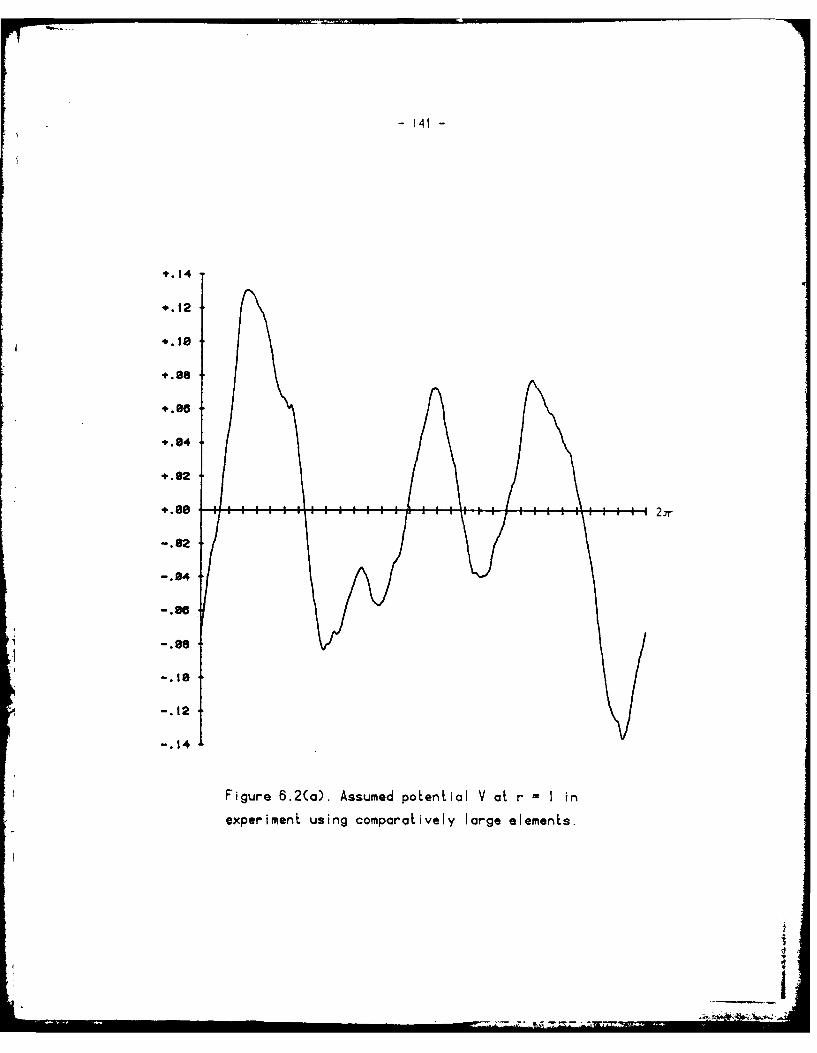
- 141 -
•.14
+.12
+.08
4.84
+..92
+.08 .-.. t..- . -. . . .--.- . .-1 - 2.7
-.924
-. 88
-. 90
-. 04
-. 12
-. 14
Figure 6.2(c). Assumed polential V at r = I in
experimen using comparatively large elements.
______ 4

-142-
+.14
+. 12
+.84
+.92
.. 9. . . . . . . . . .
+.s ..82.. 2
-. 02
-. 04,
-. 06
-. 12
-. 14
Figure 6.2(b). Calculated potential V at r =I in
experiment using comparatively large elements.
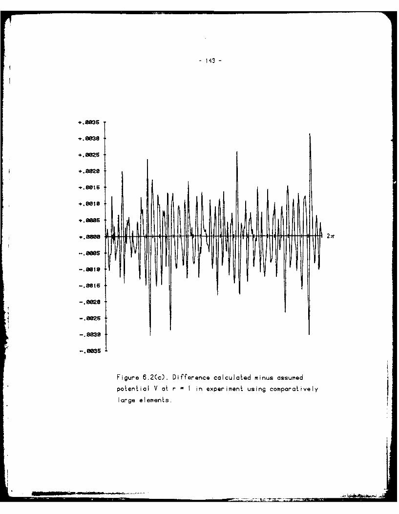
- 143 -
.,8835
.0825
+.8828
-. Owt5
+. Sao816
-. 8081
-. O1t
-. 8838,
-. 885
Figure 6.2(c). Difference calculated minus assumed
potential V at r = I in experiment using comparatively
large elements.
OEM-i

- 144 -
*.12
91
.92
-. 84
-.06
-.1
-. 12
-. 14
Figure 6.2(d). The assumed field V at r I truncated to
circular harmonics of degree n < 32. Experiment using
comparatively large elements.
l!

1 45-
+.gals
+. 8065
-. 806
-. 9I
-.9918
-. 03
-. 03
Figure 6.2(e). Contribution of circular harmonics of
degree ni > 32 to the assumed field V at r 1 . Experiment
using comparatively large eiemenLs.
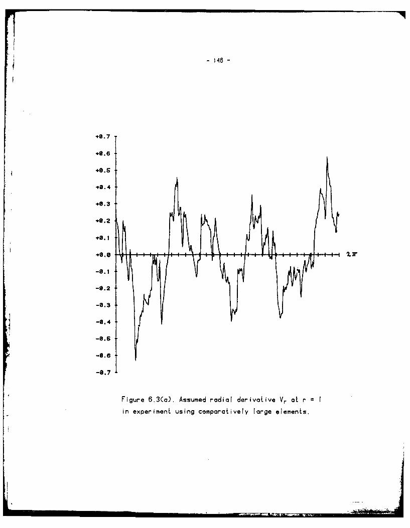
1 t46 -
.9.7
+0.6
+8.5
+ 8.4
-0.39.2
-8.3
-~0.4
.9.2
-8.2
-8.3
-8.7
~-0.6
-0.7
Figure 6.3(a). Assumed radial derivative Vr at r =I
in experiment using comparatively large elements.

+-147-
.9.2
+.94r
.9.2
-6.3
-9.4
-6.5
Figure 6.3(b). Calculated radial derivative Vr at r =I in
experiment using comparatively large elements.

- 148 -
*.eeII j
+.19
Figure 6.3(c). Difference calculated minus assumed
radial derivative Vr at r = I in experiment using
comparatively large elements.

9.S. . . . . . . * 8.8.4
49.1
-0.4
-0.6
Figure 6.3(d). Radial derivative Vr of the assumed field
at r = I, truncated to circular harmonics of' degree n 4 32.
Experiment using comparatively large elements.

-* gso -
+.96
-. 16
Figure 6.3 (e). Contribution of circular harmonics of4degree n > 32 to the radial derivative Vr of the assumed
field at r = 1. Experiment using comparatively large
elements.
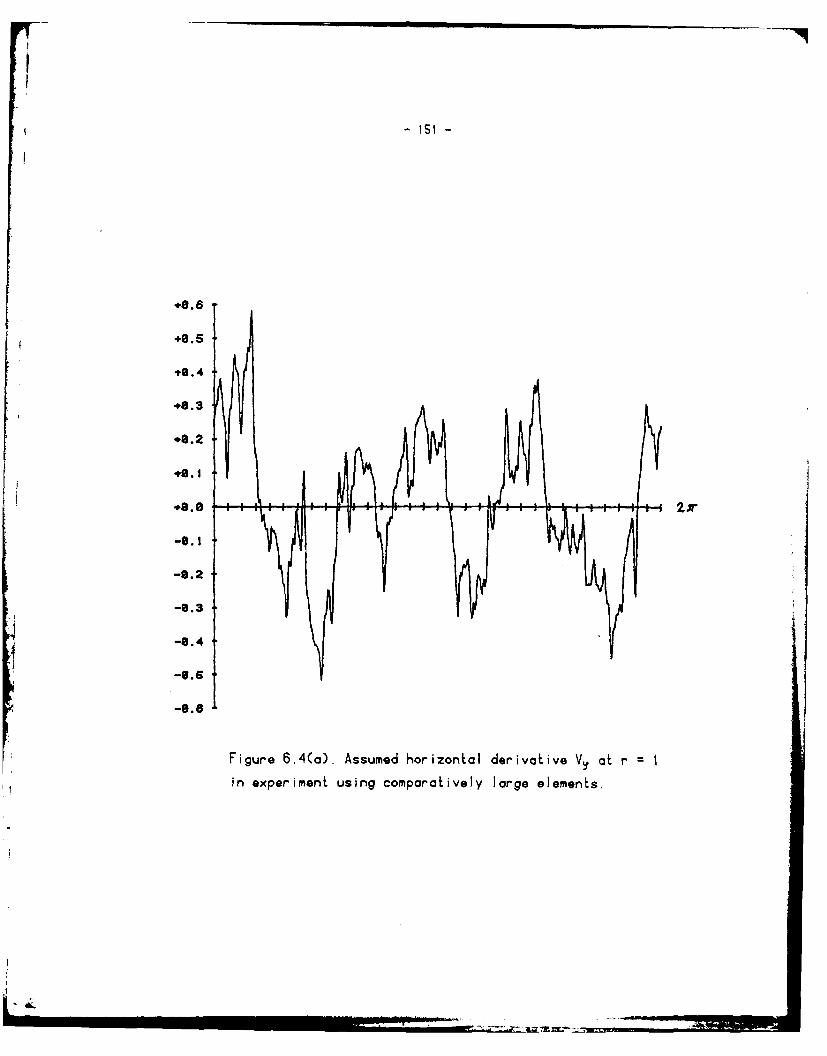
+0.5
iS0.4
+.02 i j
-9.2
-8.3
-8.4
-8.6
Figure 6.4(o). Assumed horizontal derivative Vy at r=
in experiment using comparatively large elements.

-152-
+0.3
+9.2
-9.2
-8.3
-0.6
Figure 6.4(b). Calculated horizontal derivative VI, at
r I in experiment using comparatively large elements.

-153-
-.20
Figure 6.4(c). Difference calculated minus assumed
horizontal derivative V? at r I in experiment using
comparatively large elements.

.0.4
+..
.2
+.9r j
-9.2
-9.3
-0.4
-6.8
-6.7
Figure 6.5. Superposition of assumed and calculated radial
derivative V1. at r =I in experiment using comparatively
large elements.

+7
+6
+4
+3
.2
-1
-2
-3
Figure 6.6. Calculated Loplacean LW at r I in
experimnent using comparatively large elements.

- 156 -
In order to put the potential derived from finite elements to a further
test, a number of orbits of passive mass-points was numerically
integrated. A reference potential equal to
U(r) - Log -7 (6.10)
was assumed. If VAss(r,p) and VCLjr,y) denote the assumed and calculated
potential discussed previously, then the total potential used in the
orbit calculations was either
WASS Ur(c) LIUr) + co~s(n ) (6.lla)
or
WCLC(rc?) ' 1(r) + c.V,,, (r.y) c6.lb)
By choosing
Co a .0003
an attempt was made to relate the reference potential and the disturbing
potential in a way quantitatively similar to the real earth.
The equation of motion in polar coordinates is
""0 r+ . r aw
rq4 31 '(6.12)
For near circular orbits one may represent r and p in the following way:
r, r. + Ar(6.13)
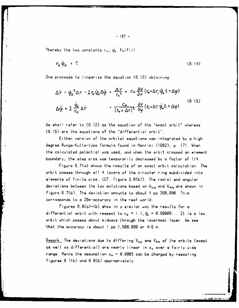
- 157 -
Thereby the two constants ro, 4'o fulfill
r. 0 (6.14)
One proceeds to linearize the equation (6 12) obtaining:
(6. r)4.2Lr C0(gL + *o r(r+L.
noc (r0.. (rY
We shall refer to (6.12) as the equation of the 'exact orbit" whereas
(6.15) ore the equations of the 'differential orbit".
Either version of the orbital equations was integrated by a high
degree Runge-Kutta-type formula found in Henrici (1962), p. 171. When
the calculated potential was used, and when the orbit crossed an element
boundary, the step size was temporarily decreased by a factor of 1/4.Figure 6.7(a) shows the results of an exact orbit calculation. The
orbit posses through all 4 layers of the circular ring subdivided into
elements of finite size. (Cf. figure 3.6(b)). The radial and angular
deviations between the two solutions based on W, and WASSare shown infigure 6.7(b). The deviation amounts to about I pp 300,000 This
corresponds to a 20m-accuracy in the real world.
Figures 6.8(a)-(b) show in a similar way the results for a
differential orbit with respect to r0 = 1.1,4. = 0.90909... It is a low
orbit which posses about midways through the lowermost layer. We see
that the accuracy is about I pp 1,500,000 or 4-5 m.
Remark: The deviations due to differing V, ans VA, of the orbits (exact
as well as differential) are nearly linear in c. over a fairly wide
range. Hence the assumption co = 0.0003 can be changed by rescaling
figures 6.7(b) and 6.8(b) appropriately.
_ I
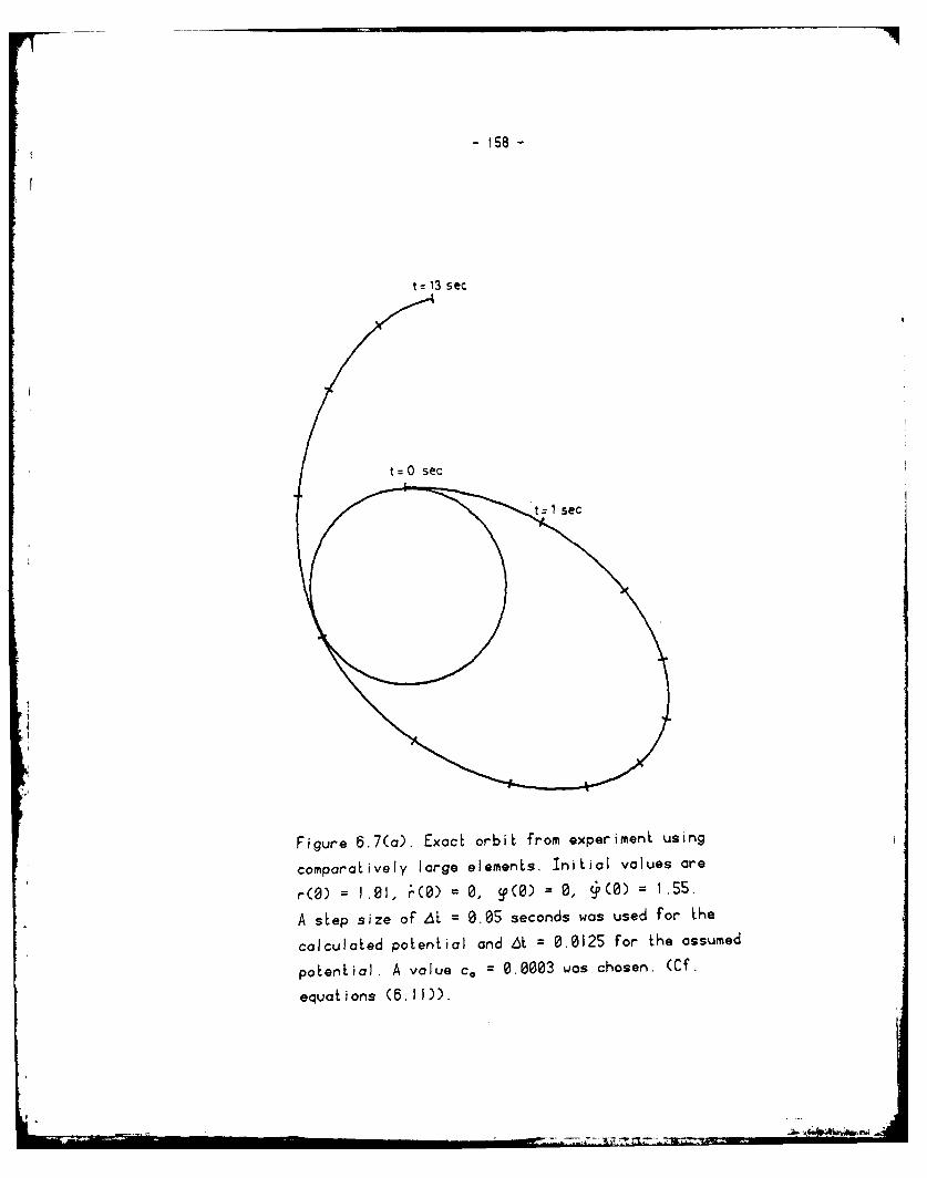
- 158 -
t 13 sec
t=0 sec
t 0sec
Figure 6.7(a). Exact orbit from experiment using
comparatively large elements. Initial values are
r(O) = 1.01, ?(O) = 0, S() = 0, (O) = 1.55.
A step size of AL = 0.05 seconds was used for the
calculated potential and 6t = 0.0125 for the assumed
potential. A value c. 0.0003 was chosen. (Cf.
equations (6.11)).
Mr-

*.998189
~emses
W:3 sec
+.89089
-.. 900985
awe. 903
+. meson
Figure 6.7(b). Difference in r (Lop) and y (bottom)
from calculated and assumed potential. Experiment
using comparatively large elements.
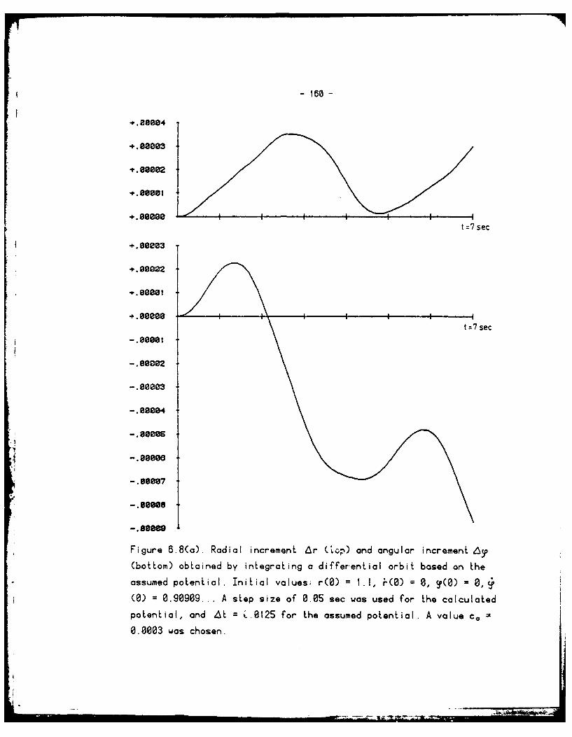
- 166 -
-.08004
+.08003
t =7 sec
S,+. 0003
".09022
t :7 sec
-. 9001
-. 90092
-. 00003
-. 99094
-. 89095
-. 00007
-. 9907
~-. 99088
-. Sam99
Figure 6 .8(a). Radial increment 6r (..) and angular increment L50
(bottom) obtained by integrating a differential orbit based on the
assumed potential. Initial values: r(O) = 1.1, K(O) = 0, 9() = 0,
(0) = 0.90909... A step size of 0.05 sec was used for the calculated
potential, and At = L.0 125 for the assumed potential. A value c. =
0.0003 was chosen.

- 161 -
!M
t =7 sec-. 8888881
-.00802
-. 8888003
+.0eseei. 8888
+.08088097
+. 880098.. 988884
+.G88MS92
+. 0808081
+. 88988
r t =7 sec
Figure 6.8(b). Difference in 6r (top) cnd 69, (bottom)
of differential orbits based on calculated and assumed
potential. Experiment using comparatively large elements.

- 182 -
Remark: Note that orbits in a central force field implied by (6.10) are
not closed. In case of the differential orbit, the angle between
successive pericenters (successive apocenLers) is given by (cf. Arnold
(1978), p. 37, problem 2)
ir (6.16)
Translated into time this gives
. 9 sec (6.17)
This is in agreement with figure 6 .8(a).
We summarize some further results of this experiment in tables 6.2
and 6.3. Table 6.2 lists the magnitude of the nodal parameters and the
magnitude of the deviations between calculated and assumed field.
Maximal and rms quantities are listed per level. There are 7 levels of
nodes. A layer of simple quads is bounded by two levels. A layer of
compound quads has one additional level of nodes halfways between the
two bounding levels. Level I corresponds to r I, level 7 to
r = r r 3.55884 ....
__________ !
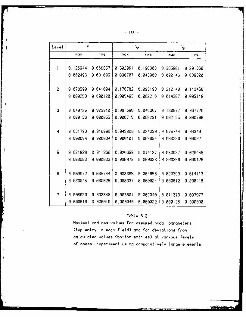
163 -
Level V V V91
max rms max rms max rms
0.126944 0.066857 0.5029&1 0.198303 0.365901 0.201368
0.002493 0.001005 0.098707 0.043960 0.092146 0.039320
2 0.078590 0.041004 0.178782 0.093193 0.212148 0.113458
0.000258 0.000128 0.005493 0.002216 0.014307 0.005119
3 0.049725 0.025910 0.08696 0.046367 0.130977 0.067720
0.000136 0.000055 0.000715 0.000291 0.002135 0.000799
4 0.031793 0.016990 0.045800 0.024350 0.075744 0.043491
0.000084 0.000034 0.000101 0.000054 0.000380 0.000221
5 0.021928 0.011866 0.026655 0.014127 0.050927 0.029458
0.000093 0.000033 0.000075 0.000038 e.000256 0.000126
6 0.009972 0.005744 0.008395 0.004658 0.020399 0.014113
0.000045 0.000026 0.000037 0.000024 0.000612 0.000418
7 0.005620 0.003345 0.003601 0.002040 0.011373 0.0079770.000016 0.000010 0.000040 0.000022 0.000126 0.000090
Table 6.2
Maximal and rms values for assumed nodal parameters
(top entry in each field) and for deviations from
calculated values (bottom entries) at various levels
of nodes. Experiment using comparatively large elements.

-164-
Table 6.3 compares some of the assumed potential coefficients an, bn;
n 2, ..., NHARM 8 with Am, B, obtained by the collocation procedure
at r row,
SA, B,
n a, bn
Diff. Diff.
-0.016589 0.051241
2 -0.016752 0.051S70
0.000163 -0.000329
-0.054197 0.041178
3 -0.055401 0.042326
0.001204 -0.001148
-0.000030 0.015842
4 0.0663t3 0.019369
-0.000343 -0.003527
(the remaining coefficients are not listed
because the errors are comparable in size
to the coefficients themselves)
Table 6.3
Comparison of assumed (top entries) and calculated(middle entries) harmonic coefficients. Experiment
with comparatively large elements.

- 16S -
6.3.2. An experiment usinQ comparatively small elements.
The input parameters were specified as follows
IDEGR = 3 [same as before]
ISWINF = 2 [same as before]
NLAYER = 4 [same as before]
ITYPE(I) = I [same as before]
ITYPE(2) = 1 [same as before]
ITYPE(3) = 2 [same as before]
ITYPE(4) = 2 [same as before]
NELEM(I) = 128 [increased by a factor of 4]
HFCT 1 [same as before]
NPOTC : 64 [decreased by factor 1/2]
DAMP I I [less damping than before]
NPINST = 8 [same as before]
STKWGT = 5 [same as before]
NHARM : 32 [increased by a factor of 4]
NPINHA 8 [same as before]
HARWGO 50 [same as before]! HARWGI S [same as before]
Table 6.4 and figure 6.9 illustrate the geometry of the element
partition. Note that r,. results in a smaller value than before.
t

- 166 -
LAYER ITYPE NELEM RADIUS DELPHI
1 1 128 1.00080 0.04909
2 1 128 1.04909 0.84909
3 2 64 1.10058 0.09817
4 2 32 1.28863 0.19635
, 1.44595
Table 6.4. Element partition in experiment using
comparatively small elements.
We now exhibit without much text the counterparts of figures 6.2-6.4,
6.7-6.8 and tables 6.2 and 6.3. These are the figures 6.10-6.14 and the
tables 6.5-6.6.
.11
Figure 6.9. Element partition for experiment
using comparatively small elements.
4.I~

- 167 -
+~.4
°4.
+.2
-. 2
-. 3
-. 4
-. 001
-. 683
Figure 6.10. Assumed po.en8ia{ V (Lco) of r I in experiment using
comparatively small elements. The calculated V is graphicalliyindistinguishable. The bottom figure shows the enlarged diference
coalculated minus assumed V.indstngishbl. he otomfiureshwstheenared ifernc

- 63 -
+.08
*.16
+.4
.2 f
.0
-2
-4
+ .84
-. 82
-. 04
-. 00
-. 96
Figure 6.11. Assumed radial derivaLive Vr (Lop) at r I in experiment
using comparatively small elements. The calculated V, is graphically
nearly indist;nguishable The bottom figure shows the enlarged
difference calculated minus assumed V, at r = 1.
a., t

+4
+2
+08
-2
-4
+.3I
-.2
-. 4
Figure 6.12. Assumed angular derivative VT (Lop) at r I
in experiment using comparatively small elements. The
calculated V, is not shown. The bottom figure shows the
enlarged difference calculated minus assumed V? at r = 1.
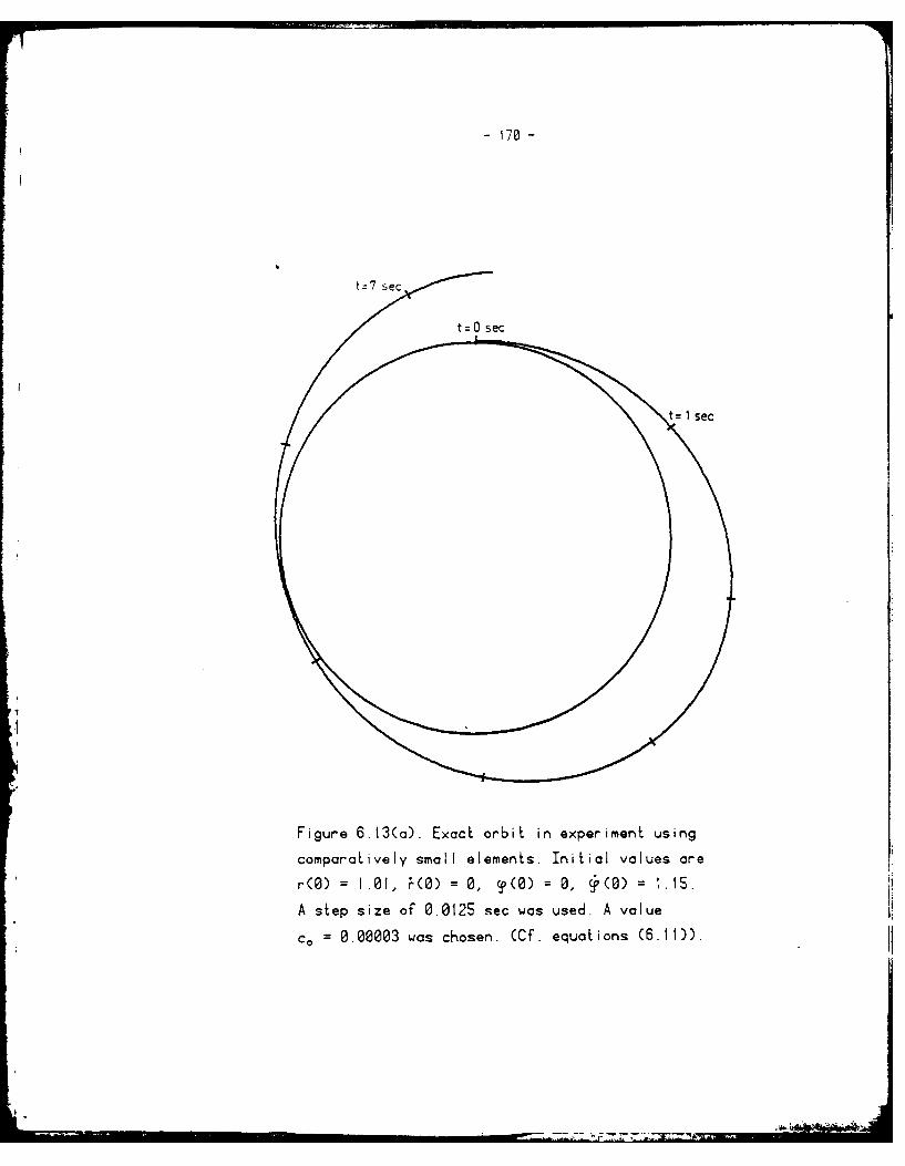
-170-
Figure 6.13(a). Exact orbit in experiment using
comparatively small elements. Initial values are
r(O) = 1.01, (O) =0, T(O) =0, (O) =1.15.
A step size of 0.0125 sec was used. A value
c= 0.00003 was chosen. (Cf. equations (6.11)).

- 171 -
*.89sSe7.smsse
*.0050ma t7 e
*.09000084
*.seem se
* .sam t3s- eseeme 12se
899880 t I
- .050M94
* 98MOS+.Gamas1
* *asess s* . sesssei
Fiur 6.3() Difssens inr(op n (otm
ofeac rbt otindfrmcaclae adasuepoesssteta.Eprmn usn coprtvl sm l
*.elements
7~~ ~ ~ -7 sec77Z:Z

-172 -
+.eaeles
+. 899998
-. Bosom5-. 80815e
easels
-. 989029
-. 89082S
Figure 6.14(a). Radial increment E r (op) and angular
increment 6y (bottom) obtained by integrating a
differential orbit based on the assumed potential. Initial
values were r(O) = I.1, i(O) = 0, S(0) = 0, (O) =
0.90909... A value c0 = 0.00003 was chosen. Experiment
using comparatively small elements.

-173-
tz 7sec
t 7 sec
-. 00 aei
Figure 6.14(b). Difference in 6ar (top) and dy (bottom)
of differential orbits based on calculated and assumed
potential. Experiment using comparatively small elements.

-174-
Note that the assumed potentials are different in the examples described
in the previous and in this subsection. In subsection 6.3.1. we had
NPOTC = 128 coefficients in the assumed potential and a damping factor
of DAMP = 2. in this subsection NPOTC = 64 and DAMP = 1. The gradients
of the present potential are about 10 times larger at r = I than in the
earlier example. For this reason, the constant c,, of equation (6.11) was
chosen by a factor of 1/10 smaller than before. However, o remark given
in section 6.3.1. carries over, implying that the figures 6.13(b) and
6.14(b) may be rescaled in proportion to any change of c..
Due to the differences in the assumed potentials the differences
in the results are not only due to the change of the element partition.
Hence the results are not immediately compared. In the next section a
number of experiments will be described summarily. From this additional
information it may be concluded, that the transition from NELEM(O = 32
to a value of 128 improves the results by about I digit at r = 1.
Figures 6.13 and 6.14 showing the results of the orbit
calculations demonstrate an accuracy of about 1 pp S5,000,000 in case of
the exact orbit. This corresponds to 1-2 m. The differential orbit is
good to I pp 300,000,000. This correspond to 2 cm.

- 175 -
,Leve I V V, VTmeeIm rms max rms
1 0.560348 0.214973 5.990022 2.260387 6.250663 2.255706
0.002427 0 000882 0.046030 0.016975 0 328472 0.153894
2 0.384302 0.171249 2.389440 0.797211 2.324042 0.834182
0.000698 0.000250 0.053510 0.019825 0.011507 0.004792
3 0.297927 0.143964 1 .330956 0.502973 1.334445 0.553725
0.000094 0.000026 0.004152 0.001534 0.005652 0.001970
4 0.243919 0.123493 0.853614 0.368318 0.912405 0.427124
0.000053 0.000023 0.001245 0.000492 0.005634 0.001950
5 0.209708 0.107151 0.606866 0.286809 0.696430 0 348634
0.000044 0.000019 0.000588 0.000227 0.001248 0.000473
6 0.156166 0.082076 0.348728 0.184487 0.458199 0.248361
0.000091 0.000046 0.000463 0.000222 0.003435 0.001451
7 0.122152 0.064510 0.240170 0.127450 0.340255 0.187136
0.000058 0.000031 0.000102 0.000052 0.000789 0.000376
Table 6.5
Maximal and rms values for assumed nodal parameters
(top entry in each field) and for deviations from
calculated values (bottom entries) at various levels
of nodes. Experiment using comparatively small elements.
1.~

I1
- 176 -
SA, B, A, Bn 0 b, on b,
Diff. Diff. Diff. Diff.
-0,033504 0.103139 -0.005873 -0.0266462 -0 033505 0 103140 13 -0 006296 -0 027436
0.000001 -0.000001 0.000423 0.000790
-0.166199 0.126972 0 009536 0.0273543 -0.166203 0.126977 14 0.010171 0.027769
0.000004 -0.000005 -0.000635 -0.000414
0.001247 0.077468 -0 001018 0.0252604 0.001250 0.077477 IS -0.000838 0.025864
-0.000003 -0.000009 -0.000180 -0.000604
-0,035952 -0.058543 -0.013724 -0.0103415 -0,035958 -0.058558 16 -0 013725 -0 011124
0.000006 0.000015 0.000001 0.000783
0.023489 0.072583 -0.007358 -0.0081606 0.023507 0.072625 17 -0.007605 -0.007283
-0.000017 -0.000042 0.000247 -0 000877
-0.025322 -0.013856 -0.019404 -0.0153087 -0.025337 -0 013859 18 -0.020553 -0.014436
0.000015 0.000003 0.001149 0.000872
0.031356 -0.051497 0.022968 -0.0189578 0.031431 -0.051597 19 0.023800 -0.020617
-0.000075 0.000100 -0.000832 0.0016600.052027 -0.032417 -0.012259 -0.015923
9 0.052222 -0.032523 20 -0.012340 -0.016005
-0.00019S 0.000106 0.000081 0.000082
0.003373 0.017371 -0.001372 0.00783810 0.003460 0.017520 21 -0.001379 0.007600
-0.000087 -0.000149 0.000006 0.080238
0.012190 0.018735. -0.020856 0.013256II 0.012312 0.018955 22 -0.019737 0.011703
-0.000122 -0.000220 -0.001119 0.001553
0.000715 -0.001960 -0.004177 0.00574412 0.000830 -0.002129 23 0.000844 0.008234
-0.000016 0.000169 -0.005021 -0.002490
Table 6.6Comparison of assumed (Lop entries) and calculated(middle entries) harmonic coefficients. Experimentusing comparatively small elements.
.4i

- 177 -
5.4. Summary of other experiments.
6.4.1. Experiments using bicubics
Table 6.7 lists input parameters and resulting accuracies for a number
of experiments using bicubics.
Experiment 1 2 3 4 5 6 7 8 9
ISWINF 1 1 1 2 I 2 1 1 1
NLAYER 4 4 4 4 4 4 5 4 4
ITYPE(1) I I I I I I I I I
ITYPE(2) I I I I I I I I I
ITYPE(3) 2 2 2 2 2 2 2 2 2
ITYPE(4) 2 2 2 2 2 2 2 2 2
ITYPE(S) / / / / / / 2 / /
NELEM(I) 32 32 32 32 32 64 64 128 t28
HFCT I 1 I I I I 0.75 I I
rur 3.56 3.56 3.56 3.56 3.56 2.01 2.72 1.45 1.45
NPOTC 16 32 128 128 128 32 64. 64 128
DAMP 1 1 2 2 1 1 1 1 1
NPINST 8 8 8 8 8 8 8 8 8
STKWGT 5 5 5 5 5 25 5 5 5
NHARM 8 8 8 / 8 / 8 32 32
NPINHA 8 8 8 / 8 / 8 8 8
HARWGO 50 50 50 I 50 / 50 50 so
HARWGI is is5 / 5 / 5 5 5
(table continued on next page)
A1
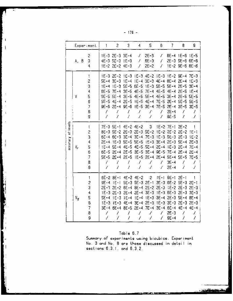
1 78-
Experiment 1 2 3 4 5 6 7 8 9
2 IE-3 2E-3 3E-4 / 2E-3 / 8E-4 IE-6 IE-5A, B 3 4E-3 SE-3 I E-3 / 6E-3 / 2E-3 5E-6 6E-6
4 1 [-2 2E-2 4E-3 / 2E-2 / 1 E-2 9E-6 8E-6
I 1 [-3 2E-2 I E-3 I E-3 4E-2 i E-3 I E-2 9E-4 7E-32 SE-A 3E-3 i [-4 I [-4 3E-3 4E-4 8E-4 2E-4 I E-33 iE-4 iE-3 5E-S 6E-S IE-3 5E-5 5E-4 2E-5 3E-44 8E-5 7E-4 3E-5 4E-5 7E-4 4E-5 4E-4 2E-5 IE-4
V S 9E-5 SE-4 3E-5 4E-5 5E-4 4E-5 3E-4 2E-5 5E-56 SE-S 4E-4 2E-5 IE-S 4E-4 7E-5 2E-4 SE-S SE-S7 9E-6 2E-4 9E-6 I E-S 3E-4 7E-5 2E-4 3E-5 3E-5
8 / / / 2E-4 / /9 / / / 9E-5
1 7E-3 SE-i 4E-2 4E-2 3 1E-2 7E-1 2E-2 I2 8E-3 5E-2 2E-3 2E-3 5E-2 IE-2 2E-2 2E-2 IE-13 6E-4 6E-3 3E-4 3E-4 7E-3 I E-3 5E-3 2E-3 i E-24 2E-4 I E-3 SE-S SE-S I [-3 3E-4 2E-3 SE-A 2E-3
Vr S I E-4 SE4 4E-5 4E-5 5E-4 2E-4 I E-3 2E-4 7E-46 6E-5 2E-4 2E-5 3E-5 3E-4 9E-S 7E-4 2E-4 2E-47 SE-S 2E-4 2E-5 I E-5 2E-4 2E-4 SE-A 5E-S 7E-58 / 3E-4 / /9 / 2E-4
.1I 6E-2 8E-I 4E-2 4E-2 2 IE-1 9E-1 2E-1 I2 9E-4 IE-I 5E-3 5E-3 2E-I 3E-3 6E-2 SE-3 2E-1.13 2E-3 2E-2 8E-4 8E-4 2E-2 2E-3 IE-2 2E-3 2E-34 I E-3 2E-3 2E-4 2E-4 3E-3 I [-3 6E-3 2E-3 3E-3
V, S SE-A 1 E-3 I E-4 I E-4 1 E-3 3E-4 2E-3 SE-A 8E-46 IE-3 1E-3 4E-4 31E-4 2E-3 IE-3 3E-3 2E-3 2E-37 3E-4 6E-4 8E-5 2E-4 7E-4 3E-4 6E-4 4E-4 4E-48 / 2E-3 / /9 / / 9E-4
Table 6.7Summary of experiments using bicubics. ExperimentNo. 3 and No. 8 are those discussed in detail insections 6.3.1. and 6.3.2.
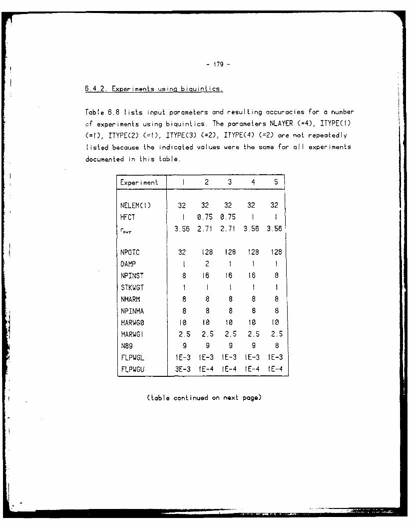
- 179 -
6.4.2. Experiments using biquintics.
Table 6.8 lists input parameters and resulting accuracies for a number
cf experiments using biquintics. The parameters NLAYER (=4), ITYPECI)
(=1), ITYPE(2) (=t), ITYPE(3) (=2), ITYPE(4) (=2) are not repeatedly
listed because the indicated values were the same for all experiments
documented in this table.
Experiment I 2 3 4 5
NELEM(I) 32 32 32 32 32
HFCT I 0.75 0.75 I I
rvr 3.56 2.71 2.71 3.56 3.56
NPOTC 32 128 128 128 128
DAMP I 2 1 1 1
NPINST 8 16 16 16 8
STKWGT I I I I I
NHARM 8 8 8 8 8
NPINHA 8 8 8 8 8
HARWGO 10 10 10 10 to
HARWGI 2.5 2.5 2.5 2.5 2.5
N89 9 9 9 9 8
FLPWGL IE-3 IE-3 IE-3 IE-3 IE-3
FLPWGU 3E-3 IE-4 IE-4 IE-4 IE-4
(table continued on next page)
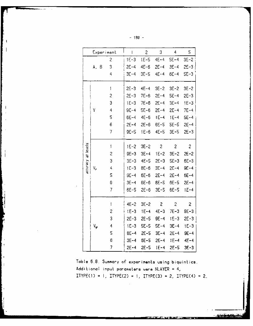
180-
Experiment 1 2 3 4 S
2 1E-3 1E-5 4E-4 SE-4 3E-2
A, 8 3 2E-4 4E-6 2E-4 3E-4 2E-3
4 3E-4 3E-S 4E-4 6E-4 5E-3
1 2E-3 4E-4 3E-2 3E-2 3E-2
2 2E-3 7E-6 2E-4 SE-4 2E-3
3 IE-3 7E-6 2E-4 3E-4 IE-3
V 4 9E-4 SE-6 2E-4 2E-4 7E-4
5 6E-4 4E-6 IE-4 IE-4 SE-4
6 2E-4 2E-6 6E-5 5E-S 2E-4
7 9E-5 IE-6 4E-S 3E-S 2E-3
1 IE-2 3E-2 2 2 2
2 9E-3 3E-4 IE-2 3E-2 2E-2
3 3E-3 4E-5 2E-3 5E-3 6E-3
Vr 4 IE-3 8E-6 3E-4 2E-4 9E-4
S 9E-4 6E-6 2E-4 2E-4 6E-4
6 3E-4 6E-6 8E-5 6E-5 2E-4
7 6E-5 2E-6 3E-5 6E-S iE-4
1 4E-2 3E-2 2 2 2
2 IE-3 IE-4 4E-3 7E-3 9E-3
3 2E-3 2E-5 9E-4 IE-3 2E-3
Vv 4 IE-3 5E-5 5E-4 3E-4 1E-3
5 8E-4 2E-S 3E-4 2E-4 9E-4
6 3E-4 6E-5 2E-4 IE-4 4E-4
7 2E-4 2E-S IE-4 2E-5 3E-3
Table 6.8. Summary of experiments using biquintics.
Additional input parameters were NLAYER = 4,
ITYPECI) = I, ITYPE(2) = 1, ITYPE(3) = 2, ITYPEC4) = 2.

- t8l -
6.4.3. Discussion.
It is interesting to compare experiments based on the some assumed
field, e.g. the bicubic-experiments 5 and 9. (The field at r = i is
shown in figures 6.10-6.12. Also table 6.5 applies to this field). It is
seen that the transition from 32 elements in the lowermost layer to 128
elements results in an increase of accuracy by one digit. On the other
hand, experiments 8 and 9 differ only with respect to NPOTC. One
recognizes that experiment 9 looses accuracy in the lower layers due to
a rougher field there. However the accuracy in the upper layers is about
the some. This confirms our reasoning that the finite element solution
regularizes the field without affecting the lower frequencies. A
comparison of experiments 3 and 4 shows that the representation of the
field in the outer zone by spherical harmonics is about equivalent to
representation by elements extending to infinity. However it must be
borne in mind that the computational effort is less in the case of
elements extending to infinity.
Experiment No. S using bicubics and experiment No. 4 using
biquintics are otherwise based mostly on equal parameters. A comparison
shows that the improvement coming from biquintics is marginal.
Experiments No. 4 and No. 5 of the biquintics-table show that
fixing the Laplacean at zero gave worse results. It is particularly
interesting how poorly the harmonic coefficients were recovered in
experiment 5. In all experiments using biquintics the recoverage of the
harmonic coefficients was inferior to that in the experiments using
bicubics. The reason is not yet completely clarified.

-182-
6.4.4. A word on the Comp~uter programs.
The programs for the Amdahl 470 V/6-II were written in an extended
FORTRAN. They comprised about 6000 statements. Double precision was used
throughout. Coding, testing and processing required about 6 weeks. No
attempt was mode to optimize speed by using assembly code in the inner
loop of the equation solver. The CPU time for the largest experiment was
83 seconds. It required the solution of a linear system with 2368
unknowns. Recherches show that about half of the time was spent on
evaluating the assumed potential and its derivatives for comparison
purposes. The time spent on the solution of the linear system must have
been less than 40 seconds. A full system of this size would have
required a CPU of more than 74 minutes. Hence a factor of about 1/100
has been gained by the nested dissection method.
The programs for the post-analysis on the WANG 2200 VP-desk-top
computer were written in an extended BASIC, called WANG BASIC-2. About
500k bytes of code were assembled requiring an effort of about 3 weeks.
Doing the post-analysis on a large computer would have required a time
span of probably 3 months. Sinall desk top computers have powerful
editing facilities, they offer instant response during editing, and
instant diagnosis during testing. It is a nonsense to solve small
problems on large computers.
6.4.5. Further desirable experi,,,ieris.
Time pressure did not allow to conduct all experiments the author had
originally in mind. It was intended to generate 'assumed potentials'
other than those defined by circular harmonics. For example it would be
interesting to see how the method performs for a potential generated by

1 83-
buried dipoles. Also ootentials with other types of near singularities
could be tried Another test could have been devoted to irregularly
distributed measurement locations, to noisy data, and to less regular
element partitions. Comparisons with the results of other methods
applied to the same 2-dimensional problem are missing. Finally, tests in
3 dimensions should be performed. Unfortunately there is a limit to the
amount of work a single person can do in a year, in addition to teaching
and administrating. It is intended to continue the experiments with the
help of my coworkers and students and to give a more complete report at
a later occasion.
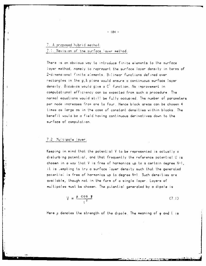
- 184 -
7 A proposed hybrid method.
7.1. Revision of the surface layer method.
There is an obvious way to introduce finite elements to the surface
layer method, namely to represent the surface layer density in terms of
2-dimensional finite elemenLs. Bilinear functions defined over
rectangles in the 9,% plane would ensure a continuous surface layer
density. Bicubics would give a C1 function. No improvement in
computational efficiency can be expected from such a procedure. The
normal equations would still be fully occupied. The number of parameters
per node increases from one to four. Hence block areas can be chosen 4
times as large as in the case of constant densities within blocks. The
benefit would be a field having continuous derivatives down to the
surface of computation.
7.2. Multipole layer.
Keeping in mind that the potential V to be represented is actually a
disturbing potential, and that frequently the reference potential U is
chosen in a way that V is free of harmonics up to a certain degree N-I,
it is 6empting to try a surface layer density such that the generated
potential is free of harmonics up to degree N-1. Such densities are
available, though not in the form of a single layer. Layers of
multipoles must be chosen. The p,Aential generated by a dipole is
2F cos (7.1)
Here . denotes the strength of the dipole. The meaning of V and I is
...........-.......-.- P

AD-Aio* 164 OHIO STATE UNI[V COLU1US DEPT OF 1OJIETIC SCIENCL /f 8/bTHE USE OF FINITE ELEMENTS IN PHYSICAL GEOOESYO(U)APR &I P HEISbL. F1928-79-C-0075
UNCLASSIFIED DOS-313 AFOL-TR-81-011 NL*3 EhIIIIIIIIEIIIIIIIl*//Iuui

~- 185 -
seen from figure 7.1point at whichV s evaluated
Figure 7.1. Explains the notation of
quantities related to a dipole
It is useful to remember that the potential of a dipole is obtained from
that one of a mass point by taking the directional derivative with
respect to the axis of the dipole and at the location of it.
cos v L (7.2)2 Bv
It follows that the potential of a dipole decreases like 0-y} as r-w.
Hence it is free of zero and first order harmonics. A dipole layer is
obtained by locating dipoles at a surface and letting the strength of
the dipole be a function of location. The axis may also vary with
location. Physically and mathematically most meaningful is the
coincidence of the axis with the surface normal. The potential of a
dipole layer is also 0(-).
Dipoles may be generalized to multipoles. Multipoles were already
studied by Gauss and Maxwell. An N+1 pole of unit strength is obtained
as
B (7.3)V! 1 v2 VN
Confer e.g. Lense (1954), p. 80 ff. Trying most simple things first, one
puts v1=V 2= . 'VN=v, thus letting the N axes coincide and obtaining
.11

- 186 -
N N (7.4)
The generated potential is O(Ti--}, i.e. it is free of spherical
harmonics up to and including degree N-1. The same holds for the
potential of a mulLipole layer. The axes may be chosen in coincidence
with the surface normal.
What is the advantage of taking a mulLipole layer instead of a
single layer? At a first glance it appears that mullipole layer also
generates a full normal equation matrix. Mind, however, that the kernel
of a mulLipole of order N+1 decreases as O(--T) as r-Of. This implies
that even for moderately large N the contribution of the multipoles
located at a small surface element decreases rapidly as one moves away
from that surfoe element. If the surface on which the mulLipole layer
is assumed is subdivided into finite elements, and if the strength
function is represented in terms of nodal parameters, then the nodal
parameters of elements at a larger distance will be coupled only by very
small coefficients which may be replaced by zeroes. Hence a sparse
system of normal equations will be obtained.
What are the difficulties to be expected in implementing the
multipole layer method, and what is an appropriate finite element
representation of the strength function? How smooth should it be chosen?
In order to give a (preliminary) answer to these questions we shall take
a closer look at spherical multipole layers in the next subsection.
7.3. Multipole layers on the sphere.
Assume a sphere of radius R = I and let r > R = I. Starting from the
well known representation for the function
with t = R2 + - 2 R r cos (7.5)

-187-
namely,
1 r > R (7.6)n=
differentiating N Limes with respect to R and putting afterwards R =,
one gets
N 1 (7.7)
ii" 1 = [ P (cos V) n(n-). ..(n-N+1) (77BRn N n r
Here Pn(t) are the familiar Legendre polynomials, normalized in a way
that Pn(l) = I. The series (7.7) converges for r > 1. Letting r--I, we
obtain in the ljmit a sequence which converges distribuLionally. The
potential generated by the multipole layer with strength function p is
V(r ) f " , R=l g(r) dF(q)fr BR N R=1R (7.8)
.1 r>R=1
Here , J are unit vectors, P is the surface of the unit sphere. We
temporarily fix r and view V(r ) as a function of only. Then (7.8)
represents an isotropic operator. According to the theory outlined in
Meissl (1971), chapter 3, we know that its eigenfunctions are the
spherical harmonics Hnm. We can calculate the eigenvalues by the
Funk-Hecke formula obtaining
=0 n(<N
= 2n+l ;n > N =0 (7.9)
%2n+ n(n-l). ..(n-N+i) nrl n N > 0
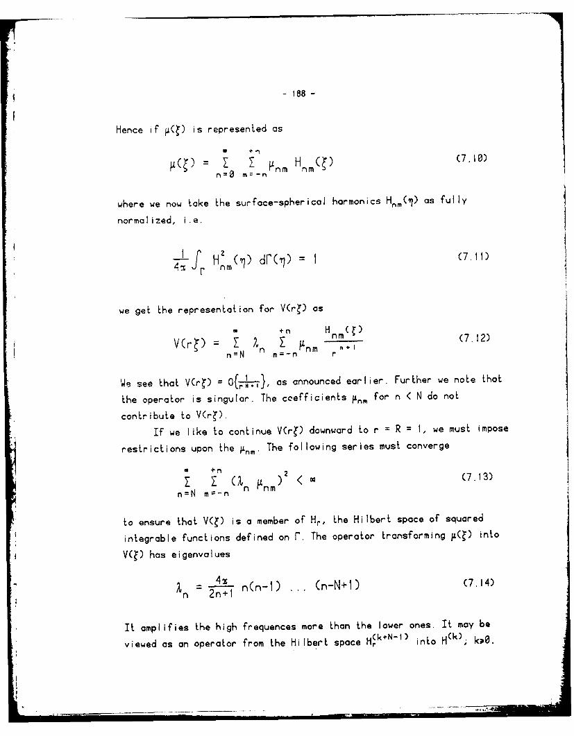
* I - 188 -
Hence if is represented as
= Hnm( ) (7.10)n=O m=-n
where we now take the surface-spherical harmonics Hm(j) as fully
normalized, i.e.
q: L f H2 (7) dF( 1 ) = 1 (7.11)
we get the representation for V(r ) as
+n H ((.nm (.2
V(r ) = I- 1 nm %In=N m=_n r
We see that V(r ) = 07-11,1} as announced earlier. Further we note that
the operator is singular. The coefficients nm for n < N do not
contribute to V(r ).
If we like to continue V(rZ) downward to r = R = I, we must impose
restrictions upon the n.' The following series must converge
Z U n Pnm ) < (7.13)
n=N m=-n
to ensure that V( ) is a member of Hr, the Hilbert space of squared
integrable functions defined on F. The operator transforming p( ) into
V( ) has eigenvalues
=42n l n(n-1) ... (n-N+1) (7.14)
It amplifies the high frequences more than the lower ones. It may be
viewed as an operator from the Hilbert space H(k N-l) into H(k); k;,.

- 189 -
The space Hr comprises those functions
S +n
f I Cnm Hnm(p (7.15)n=O m=-n
for which the following series converges
S +n t 2
1 (n c) < (n=O m=-n am
In a least squares approach we like to have at r = I a potential(2 C(N+I)V( ) e H.2 ) Hence g( ) e Hr appears appropriate. Therefore the
trial functions should be CN across element boundaries. In a Ritz-type
approach V( ) e H 1), (Z) e HrN ) and CN-1 continuity across element
boundaries would be sufficient.
Remark: One could avoid the smoothness requirements on (t) by the
Bjerhammar-sphere approach. A sphere of radius I-c is placed
concentrically into the unit sphere. The density F is assumed on this
sphere. We thus consider an operator
- V( ) (7.17)
whose eigenvalues are
47.
n =2n+' n(n-1) (718(n-N+I)(-)-
n N
However, in the present context we do not propose to shove difficulties
under the carpet by burying the mulLipole layer underneath the surface
of computation.
Suppose now, for the moment, that in (7.8) V(r ) is specified and
that p(j) is sought. If the equations are discretized in some way, we

- igg -
expect them to be very ill conditioned due to the differences in size of.
the eigenvalkies In, While the hiqh frequent components of F(j) appear to
be well determined, the low frequent components are not.
In physical geodesy we do not start from a known V(C). Instead we
have a discrete set of measurements corresponding to functionals of
V( ). The situation is more difficult but nevertheless similar. The
linear system leading Lo ( ) will be ill conditioned.
One may adopt the viewpoint that ill conditioning is equivalent to
an inproper problem formulation, and one may simply abandon the outlined
approach. On the other hand, if insight teaches one that the effects of
the ill-conditioning on the final result will be negligible, one may find
a way around the numerical difficulties. Of course, there is no hope
that insight can be replaced by calculus.
At the present time, no definite answer can be given. More time
is needed to think about the method and to conduct numerical
experiments.
• i
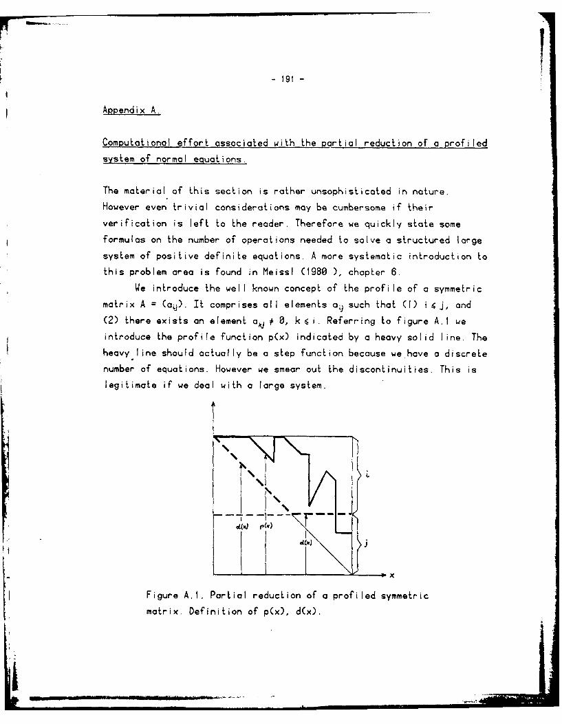
- 191 -
Appendix A.
Computational effort associated with the partial reduction of a profiled
system of normal equations.
The material of this section is rather unsophisticated in nature.
However even trivial considerations may be cumbersome if their
verification is left to the reader. Therefore we quickly state some
formulas on the number of operations needed to solve a structured large
system of positive definite equations. A more systematic introduction to
this problem area is found in Meissl (1980 ), chapter 6.
We introduce the well known concept of the profile of a symmetric
matrix A = (a). It comprises all elements aj such that (1) i4 j, and
(2) there exists an element aj # 0, k i. Referring to figure A.1 weintroduce the profile function p(x) indicated by a heavy solid line. The
heavy line should actually be a step function because we have a discrete
number of equations. However we smear out the discontinuities. This is
legitimate if we deal with a large system.
%
_ 4%
X
Figure A.I. Partial reduction of a profiled symmetric
matrix. Definition of p(x), d(x).

- g2 -
The portion below the main diagonal is not shown in figure A.I. Due to
symmetry, there is no need to store these coefficients in the computer.
The upper portion of the system comprises i equations. They are
called 'interior'. The equations below labeled j are called 'junction
equations". During partial reduction, the interior equations are
eliminated. One obtains a system of j partially reduced junction
equations.
If the matrix is split as
A A %, A% (A.1)
then the matrix of the partially reduced set is given by
A P ) A ' A (A.2)
A direct elimination procedure is used such as Gauss, Cholesky or one of
the variants. The partial triangular decomposition phase is by far most
time consuming. During this phase zero coefficients are enforced below
the main diagonal positions of he interior equations. Focus attention
on a row of coefficients whose diagonal position is implied by column x.
Call this the row x. Let y be a column to the right of x. From the
coefficient in row x and column y as many multiples of coefficients
located above it are subtracted as the following expression indicates:
x: y) - M in f Hwy ( p(-) - c()) 0), cue( p~y) - cv).o)) (A.3)
Thereby d(x) is the function implied by the heavy broken line in figure
A.l. Hence partial triangular decomposition requires
iZ.j '4.j
f d: y) cty (A.4)0

- 93 -
steps. One step comprises one multiplication and one addition. There
are also divisions and square roots (in case of Cholesky), but their
number is negligible. Also the number of operational steps involving
the right hand side, as well as the number of steps arising during the
later back-substitution phase are negligible.
Take a fully occupied system. We find
L L" Zj LEoj
, r L , 0 + (A.5)
0 x X
This formula is frequently used in chapter 4. For j = 0, i.e. full
reduction, we obtain
(A.6)
z,6

- 194-
References
Ahlberg J. H.; E. N. Nilson, J. L. Walsh (1967): The theory
of splines and their applications. Academic Press, XI +
284 pp.
Arnold V. i (1980): Mathematical methods of classical
mechanics. Graduate texts in Mathematics, No. 60, second
corrected printing. Springer Verlag. X + 462 pp.
Avila J.; B. Malloy; J. Tomlin (1978): Use of the ILLIAC IV forthe readjustment of the North American Datum. Technical
Memorandum No. 5732, Institute for Advanced Computation,
Sunnyvale, Calif. 94085, 87 pp.
Bitmead R. R.1 B. P. 0. Anderson (1980): Asymptotically fast
solutions of Toepiitz and related systems of linear
equations. Linear Algebra and its applications. Vol. 34,
pp. 103 to 116.
Bjerhammar A. (1964): A new theory of geodetic gravity. Trans.
Roy. Inst. Technoi., 243, Stockholm.
Bjerhammar A. (1978): A review of discrete methods in PhysicalGeodesy. In Moritz-Suenkel (ed.): Approximation methods
in Gravity. Wichmann, Karlsruhe, pp. 211 to 233.
Boehmer K. (1974): Spline-Funktionen. Teubner Studienbuecher,
Teubner Stuttgart. 340 pp.
Bosman E. R.; D. Eckhart. K. Kubik (1972): Delft - a
programme system for surface approximation. Bildmessung
und Luftbildwesen, Vol. 1972, pp. 13 to 20.
Brent R. P., F. G. Gustavson, D. Y. Y. Yun (1983): Fast
computation of Pade approximants and the solution ofToeplitz systems of equations. Res. Rep. RC 8173 (34952),
IBM Research Center, Yorktown Heights, NY.
- .... _ _ _ _ _ _ tL

lg Ig-
Ciarlet P. G. (1978)- The finite element method for ellipticproblems. North Holland Publ. Co., XII + 530 pp
Colombo 0. L. (1980): Optimal estimation from data regularlysampled on a sphere with applications in geodesy. Airforce geophysics laboratory TR-79-0227. Massachusetts.
Davis T. M.; A. L. Kontis (1970): Spline interpolationalgorithms for track-type survey data with applicationsto mean gravity anomalies. Technical report TR-226,Naval oceanographic office, Washington, D. C. 20390.
Douglas B. C., C. C. Goad; F. Morrison (1980): Determinationof the geopotential by satellite tracking data. J. ofGeophysics. Vol. 85, No. B10, pp. 5471 to 5480.
Engels R. C.; J. L. Junkins (979): Local representation ofthe geopotential by weighted orthonormal polynomials.17th Aerospace sciences meeting. New Orleans, January15-17.
Engels R. C.; J. L. Junkins (1979)- Finite element models ofthe earth's gravity field. Phase IV Dep. of Engin. Sci.and Mechanics. Virginia Polytechnic Instituteand State University. Blacksburg, Virginia.
Forsberg R.; C. C. Tscherning (1980): The use of height data ingravity field approximation by collocation. Preprint.Geodetic Institute Charlottenlund, Denmark.
Forsberg R.; F. Madsen (1980): Geoid prediction in northernGreenland using collocation and digital terrain models.Preprint (to be presented at the symposium 'Space Geodesyand its Applications', Cannes, November 1980). GeodeticInstitute Charlottenlund, Denmark.
Freeden W. (1978): An application of a summation formula tonumerical computation of integrals over the sphere. Bull.Geod., vol. 52, pp. 165 to 175.

~- 96 -
Freeden W (1979): Ueber eine Kiasse von integra;formeln der
Physikaischen Geodaesie. VeroeffenL;ichungen desGeodaetischen InstiLuts der Rheinisch-WestfaelischenTechnischen Hochschule Aachen, Nr. 27, 1979. ISSN 0S15-
0574.
Freeden W. (1980a) Eine Kiasse von Kubaturformeln derLinheitssphaere. Manuscript submitted to Zeitschrift fuerVermessungswesen.
Freeden W. (1980b)- Ueber die Gauss'sche Methode zurangenaeherten Berechnung von Integralen. Manuscriptsubmitted to Mathematical methods in the applied sciences.
Freeden '4. (1981): Least squares adjustment and smoothing bysplines. Manuscript submitted to manuscripta geodetica.
George A. (1973): Nested dissection of a regular finite elementmesh. SIAM Journal of Numerical Anaiysis, 10(2), pp. 345to 363.
George A.; D. R. McIntyre (1977) On the application of theminimum degree algorithm to finite element systems.Lecture notes in mathematics No. 606, pp. 122 to 149.Springer.
Hardy R. L.; W. M Goepfert (1975): Least squares prediction ofgravity anomalies, geoidal undulations and deflections ofthe verticalwith muitiquadric harmonic functions.Geophysical Research Letters, Vol. 2, No. 10, pp. 423 to426.
Heiskanen W A.; H. Moritz (1967): Physical Geodesy.W. H. Freeman and Company. San Francisco and London.364 pp.
Heller W. G.- K. S. Tait; S. W. Thomas (!977)7 Geofast - afast gravimeLric estimation algorithm. Air forcegeophysics laboratory TR-77-0195. Massachusetts.
m1
- 197 -
Henrici P. (1962) Discrete variable methods in ordinarydifferential equations. J. Wiley & Sons, XI + 407 pp.
Jordan S. K. (1978): Fourier physical geodesy. Air forcegeophysics laboratory TR-78-0056. Massachusetts.
Junkins J. L. (1977): Development of finite element modelsfor the earth's gravity field. Phase I: Macro gravitymodel for satellite orbit integration. Rep. No.UVA/525023/ESS77/103. 27 pages.
Junkins J. L.; R. C. Engels (1979): The finite elementapproach in gravity modelling. Manuscripta geodaetlicaVol. 4, pp. 185 to 206.
Koch K.; B. Witte (1971): Earth's gravity field represented bya simple layer potential from Doppler tracking ofsatellites. J. Geophys. Res. Vol. 76(971), pp. 8471 to8479.
Krarup T. (1969): A contribution to the mathematicalformulation of Physical Geodesy. Geodetisk InstItut,Meddelelse No. 44, Copenhagen, Denmark.
Lelgemann D. (1980): Kollokation und analytische Spline-funktionen. Zeitschrift fuer Vermessungswesen, Vol,. 10,
pp. 466 to 479.
Lense J. (1954): Kugelfunktionen. Second edition. AkademischeVerlagsgesel lschaft Leipzig.
McDonald B. H.; A. Wexler (1972): Finite element solution ofunbounded field problems. IEE Transactions on microwavetheory and techniques, Vol. MTT-20, No. 12, pp. 841 to847.
McDonald 8. H.; M. Friedman; A. Wexler (1974): Variational
solution of integral equations. IEE Transactions onmicrowave theory and techniques, Vol. MTT-22, No. 3,pp. 237 to 248.
198-
Meissl P. (969): Ueber zufaellige Fehler in regelmaessigengestreckten Ketien. Zeitschrift fuer Vermessungswesen.Vol. 94(969), pp. 14 to 26.
Meissl P. (1971a): A study of covarionce functions related tothe earth's disturbing potential. Report No. 151. Dep. ofGeodetic science. Ohio State University. IV + 88 pages.
Meissl P. (1971b): Preparations for the numerical evaluation ofsecond order Molodensky-type formulas. Rep. No. 163.Dep. of Geodetic science. Ohio State University. III + 72pages.
Meissl P. (1980): A priori prediction of roundoff erroraccumulation in the solution of a super-large geodeticnormal equation system. NOAA Professional Paper 12.National Geodetic Survey, Rockville, Md. X + 128 pp.
Moritz H. (1978): Interpolation and approximation. In"Approximation methods in Geodesy' ed. by H. Moritz andH. Suenkel. Sammlung Wichmann, B. 10. H. Wichmann,
Karlsruhe.
Moritz H. (1980): Advanced Physical Geodesy. H. Wichmann,Karlsruhe. XIII + 500 pp.
Morrison F. (1980): Computing the potential and attraction of adensity layer by means of elliptic integrals. Manuscriptageodetica. Vol. 5(1980), pp. 145 to 173.
Mueller C. (1966): Spherical harmonics. Lecture notes inMathematics, No. 17, Springer-Verlag,Berlin-Heidelberg-New York.
Needham P. (1970): The formation and evaluation of detailedgeopotential models based on point mosses. Rep. No. 149.Dep. of geodetic science. Ohio State University.

- 199 -
Noe H. (1980): Numerical investigations of the problem ofMolodensky. MitLeilungen der geodaeLischen Institute derTechnischen Universitaet Graz, Nr. 30, 80 pp.
Oden J. T.; J. K. Lee (1977): Dual-mixed hybrid finiteelement method for second-order elliptic problems.Lecture notes in mathematics No. 606, pp. 275 to 291.Springer.
Oden J. T. (979): The classical variational principles ofmechanics. In: Glowinsky el al. (ed.): Energy methodsin finite element analysis. J. Wiley.
Pion T. H. H. (1964): Derivation of element stiffness matricesby assumed stress distributions. AIAA-J. 2, pp. 1333 to1336.
Rauhala U. A. (1980): Introduction to array algebra.Photogrammetric Engineering and Remote Sensing. Vol. 46,No. 2, pp. 177 to 192.
Raviart P. A.; J. M. Thomas (1977): A mixed finite elementmethod for 2-nd order elliptic problems. Lecture notesin mathematics, No. 606, pp. 299 to 315. Springer.
RaviarL P. A.; J. M. Thomas (1979): Dual finite element modelsfor second order elliptic problems. In: Glowinsky et al.(ed.): Energy methods in finite element analysis. J.Wiley.
Robertson W. M. (1978): Spherical geodetic transformations.Rep. No. 1181 of Charles Stark Droper Laboratory. MFT.vol. I and II.
Schoenberg I. J. ('1916): Contributions to the problem ofapproximation of equidistant data by analytic functionsOuart. Appl. Math. 4, pp. 45 to 99, 112 to 141.
Schwarz H. R. (1980): MeLhode der finiten Elemente. B. G.Teubner, Stuttgart. 320 pp.
- 200 -
Sjoeberg L. (1978): A comparison of Bjerhammor's methods andcollocation in physical geodesy. Rep. No 273 Dep. ofgeodetic science. Ohio State University.
Snay R. A. (1978): Applicability of array algebra. Reviews ofGeophysics and Space Physics. Vol. 16, No. 3 pp. 459 to464.
Strong G.; G. J. Fix (1973): An analysis of the finite elementmethod. Prentice Hall Inc. Englewood Cliffs. XIV + 306 pp.
Suenkel H. (1977): Die Darstellung geodoetischer Integral-formeln durch bikubische Spline-Funktionen. Mitteilungender geodaetischen Institute der Technischen UniversitoetGraz, No. 28.
Szameitat H. (1979): Modell einer elastischen Erde auf Grund-loge finiter Kugelschalenelemente. DGK, Reihe C, Nr. 249.133 pp.
Tait K. S. (1980): A fast estimation algorithm for two-dimensional gravity data (Geofast). Air force geophysicslaboratory TR-80-0016. Massachusetts.
Taylor R. L.; 0. C. Zienkiewicz (1979): Complementary energy
with penalty functions in finite element analysis. In:Glowinsky et al. (ed.): Energy methods in finite elementanalysis. J. Wiley.
Thomas S. W-, W. G. Heller (1976): Efficient estimationtechniques for integrated gravity data processing. Airforce laboratory TR-76-0232. Massachusetts.
Tong P.; T. H. H. Pian (1969): A variational principle and theconvergence of a finite element method based on assumed
stress distribution. Ink. J. Solids Structures Vol. 5,pp. 463 to 472.

- 201 -
Tscherning C. C.; R. H. Rapp (1974): Closed covarionceexpressions for gravity anomalies, geoid undulations and
deflections of the vertical implied by anomaly degree
variance models. Rep. No. 208 of the Dep. of Geod Sci.The Ohio State University, Columbus, Ohio.
Tscherning C. C. (1978): A user's guide to geopotential
approximation by stepwise collocation on the RC 4000
computer. Rep. No. 53 of the Danish Geodetic Institute,
Copenhagen.
Tscherning C. C. (979): Comparison of some methods for thedetailed representation of the earth's gravity field.
Paper presented at the General Assembly of IUGG/IAG,
Canberra, Australia, Dec. 1979.
Wagner C. A.; 0. L. Colombo (1978): Gravitational spectra from
direct measurements. Goddard space flight center.
Greenbelt, Maryland.
Werner T. (1979): Untersuchungen zur Erfassung strain-induzierter Stoereinfluesse auf Neigungsmessungen. DGK.,
Reihe C, Nr. 253, 102 pp.
Zienkiewicz 0. C. (1971): The finite element method in
engineering science. McGraw-Hill. London.
Zienkiewicz 0. C.; D. W. Kelly; P. Betters (1979): Marriage a
la mode - the best of both worlds (finite elements andboundary integrals). In: Glowinsky et al. (ed.): Energy
methods in finite element analysis. J. Wiley.
Zohar S. (1969): The algorithm of W. F. Trench. J. Assoc.
Comput. Mach., Vol. 16, pp. 592 to 601.


