
ISSN 1995-2848
OECD Journal: Economic Studies
Volume 2009
© OECD 2009
The Wage Premium on Tertiary Education:
New Estimates for 21 OECD Countries
byHubert Strauss and Christine de la Maisonneuve
OECD Economics Department, 2 rue André-Pascal, 75775 Paris Cedex 16, France, E-mail:
Hubert Strauss: [email protected]; Christine de la Maisonneuve: [email protected] Strauss was previously at the OECD Economics Department and is currently
economist at the European Investment Bank. The authors would like to thankRomina Boarini, Jorge Braga de Macedo, Jørgen Elmeskov, Michael Feiner, Bo Hansson,
Giuseppe Nicoletti, Joaquim Oliveira Martins and Jean-Luc Schneider for their commentsand input during the preparation of this study. Comments received from other colleagues
of the Economics Department were also useful. Irene Sinha and Lyn Urmston providededitorial assistance. The views expressed here are those of the authors and do not
Introduction and main findings . . . . . . . . . . . . . . . . . . . . . . . . . . . . . . . . . . . . 2
Methodological issues related to the estimation of educationalwage premia . . . . . . . . . . . . . . . . . . . . . . . . . . . . . . . . . . . . . . . . . . . . . . . . . . . . . 3
Empirical specification . . . . . . . . . . . . . . . . . . . . . . . . . . . . . . . . . . . . . . . . . . . 3Construction of empirical variables. . . . . . . . . . . . . . . . . . . . . . . . . . . . . . . . . 5
Results . . . . . . . . . . . . . . . . . . . . . . . . . . . . . . . . . . . . . . . . . . . . . . . . . . . . . . . . . 10The gross hourly wage premium per annum of tertiary
education . . . . . . . . . . . . . . . . . . . . . . . . . . . . . . . . . . . . . . . . . . . . . . . . . . . 20Comparison with other estimates in the literature. . . . . . . . . . . . . . . . 22
Conclusion . . . . . . . . . . . . . . . . . . . . . . . . . . . . . . . . . . . . . . . . . . . . . . . . . . . . . . 23
Notes. . . . . . . . . . . . . . . . . . . . . . . . . . . . . . . . . . . . . . . . . . . . . . . . . . . . . . . . . . . 23
Bibliography. . . . . . . . . . . . . . . . . . . . . . . . . . . . . . . . . . . . . . . . . . . . . . . . . . . . . 25
Annex A1. Data Sources, Sample Size and Descriptive Statistics
of the Gross Hourly Wage Rate . . . . . . . . . . . . . . . . . . . . . . . . . . . 27
1
necessarily represent those of the OECD or its member countries.

THE WAGE PREMIUM ON TERTIARY EDUCATION: NEW ESTIMATES FOR 21 OECD COUNTRIES
Introduction and main findingsThe accumulation of human capital through education and training is widely recognised
as an important driver of economic growth.1 Yet, as the decision to continue schooling beyond
the secondary level is voluntary, it depends not only on talent and inclination but also on thebalance of costs of and benefits from post-secondary education. Therefore, assessing the
returns on education is a key input for policymakers who want to bolster a country’sendowment with human capital through an increase in educational attainment.2
This study focuses on the single most important component of the private return ontertiary education, the gross wage premium. There are at least two additional reasons for
paying particular attention to wage premia. First, the wage premium earned by existinggraduates is easy to observe, so high-school leavers can be assumed to take it into account
when deciding for or against enrolment in tertiary education. Second, to the extent thatwages reflect marginal labour productivity, estimates of wage premia are sometimes used
to assess the quality of human capital in an economy with a view to correcting simplermeasures based on years of schooling or attainment levels.
The study follows an augmented Mincerian wage equation framework with the grosshourly wage as the dependent variable, estimated on individual cross-sections. The latter
are obtained from household data covering 2 to 14 survey waves for 21 OECD countries.The time period runs from 1991-2004 for the United Kingdom, from 1994-2004 for the
United States and from 1994-2001 for most other countries. The traditional Mincerequation is augmented by a number of labour market-related control variables, inter alia for
wage earners that are overqualified or under-qualified in their current occupation.
The estimations are country-specific and draw from a common sample of men and
women. Over and above the usual gender dummy in the equations, the variables foreducation and labour-market experience are interacted with the gender dummy, thereby
obtaining gender-specific results for the tertiary education wage premium, the wagepenalty on not completing upper-secondary education, and the annual labour market
experience premium. The results highlight huge cross-country differences. The gross wagepremium to tertiary education ranges from 27% for Spanish men to 90% for Hungarian and
US degree holders. Cross-country variation remains high even after accounting for theaverage duration of tertiary studies. The gross wage premium per annum of tertiary
education is found to lie in an interval from 5.5% for men in Greece and Spain as well as forwomen in Austria and Italy, to 17% for men and women in Hungary and the United States,
and for women in Ireland and Portugal.
The study is structured as follows. The second section provides a brief discussion of
methodological issues raised in the microeconomic literature on returns to education in orderto highlight the value-added of this contribution and its (data-related) limitations. The third
section presents the empirical specification of the Mincerian wage equation and in the fourth,
OECD JOURNAL: ECONOMIC STUDIES – ISSN 1995-2848 – © OECD 20092
data sources and the construction of variables are described. The penultimate section presents
the results, discussed in comparison with earlier estimates and the final section concludes.
TRIES
THE WAGE PREMIUM ON TERTIARY EDUCATION: NEW ESTIMATES FOR 21 OECD COUNMethodological issues related to the estimation of educational wage premia
Most studies on returns to education use Mincerian equations. The latter relate the logof earnings to the number of completed years of schooling and experience (often as
a quadratic term).3 While Mincer (1958) considers the wage premium to be just acompensation for working in jobs requiring longer education (the net present values of
earnings streams net of education costs being identical for all levels of education), Mincer(1974) derives a similar empirical specification from a full human-capital model building
on the theoretical work by Becker (1964) and Ben-Porath (1967).4 The original Mincerequation assumes a linear effect on earnings of each year of education regardless of the
attainment level. This study, however, allows for differential effects of upper-secondaryand tertiary education.
There are a number of issues to be borne in mind when relating the Mincerian
schooling coefficient to the causal effect of schooling on earnings (Card, 1999 and Harmon
et al., 2003). First, as an investment-decision variable, years of schooling and educationattainment should be considered as endogenous, implying a possible bias in OLS estimates
of the schooling coefficient. The endogeneity bias may arise either from unobservedvariation in ability or from unobserved heterogeneity. If those who extend education
beyond compulsory schooling have greater ability than others, the estimated Mincercoefficient is biased upwards since part of the productivity differential is actually due to
innate abilities or skills acquired outside school (ability bias). The ability bias may interactwith heterogeneous subjective discount rates that result in under-estimating the true
effect of schooling on earnings if the more impatient individuals happen to be the moreable ones (heterogeneity bias). The total direction of bias in OLS estimates is ambiguous.
There is a whole strand of the empirical literature dealing with the endogeneity bias,namely by using instrumental variables (e.g. parents’ education). This option could not be
followed in this study due to lack of data. Nonetheless, the consensus from the empiricalliterature is that this bias in the estimated Mincerian wage premium is likely to be small
(e.g. see Card, 1999, and Woessmann, 2003).
Second, if there is measurement error in the education variable (one year of tertiary
schooling representing different stocks of human capital accumulated depending on schoolquality and individual characteristics), the schooling coefficient will be biased downward.5
Third, there is also a potential endogeneity bias related to labour supply effects.Indeed, every new graduate adds to the pool of skilled workers, thereby making skilled
labour less scarce and lowering the wage premium that triggered the investment decision.6
Finally, Heckman et al. (2005) point out that using ex post estimates of earnings-schooling profiles of existing workers as a decision tool for today’s investment decision
requires stationarity of earnings across cohorts in the labour market. The latter is rejectedfor the United States on the basis of 1980 and 1990 Census data. However, in this study, a
full-fledged cohort analysis is not feasible due to the limited time coverage of the availablehousehold panel data.
Empirical specificationTertiary-education wage premia are obtained by country and year from individual
earnings data following the Mincerian approach. Estimates are based on household-level
OECD JOURNAL: ECONOMIC STUDIES – ISSN 1995-2848 – © OECD 2009 3
data for three educational attainment levels (less than upper-secondary education,
completed upper secondary education, completed tertiary education). The estimation is
THE WAGE PREMIUM ON TERTIARY EDUCATION: NEW ESTIMATES FOR 21 OECD COUNTRIES
based on hourly wages, which reflect the impact of education on productivity. Monthly orannual wages would in addition capture the effect of individuals’ decisions on working
hours. Given the only weak (positive) correlation between working time and educationalattainment it is reasonable to assume that the choice of hours worked reflects individual
preferences rather than education levels. Experience is proxied by the number of years inthe labour market rather than age, because this allows better disentangling education from
experience effects.
Household-level data allow controlling for a number of individual characteristics that
potentially affect earnings but are not directly related to tertiary education. Failing to controlfor these characteristics may induce statistical bias when estimating the effect of tertiary
education. They include gender, marital status, job tenure (in years), the type of workcontract and working in the public versus the private sector. The estimates also control for
the size of the production unit (“plant size”) as it is a well-established empirical fact thatlarge firms tend to pay higher wages than small firms. It is true that to the extent that these
other labour-market outcomes are dependent on education itself, their inclusion as controlvariables would be more controversial since they could “blur” the look at the unconditional
private returns to education. However, the correlation between attainment and non-wagelabour market outcomes is very limited.7 The final control variables are over- and under-
qualification of individuals in their current occupation. The risk that in a given yearindividuals may work in a job that does not correspond to their educational attainment is not
necessarily relevant for their decision to enrol in tertiary education, hence the mismatchbetween education and occupational status should be treated separately from the education
wage premium. Indeed, the available evidence suggests that the majority of over-qualifiedindividuals tend to move up over time into an occupational status corresponding to their
educational attainment (Dumont, 2005). On balance, controlling for over- and under-qualification tends to increase the estimated wage premia.
The econometric specification is as follows (individual indices are omitted forsimplicity):
[1]
where:
hrw = gross hourly wage
edu1, edu3 = dummies for less-than-upper-secondary and tertiary education attainment,respectively
exper = number of years of experience in the labour market
married = dummy for marital status
public = dummy for public sector job
part_time = dummy for part-time worker
tenure = number of years with the same employer
indef_cont = dummy for indefinite-term contract
funderqualioverqualifsizeplantLog
contindeftenuretimepartpublicmarried
womanexperwomanexper
womaneduwomaneduedueduchrwLog
321
87654
321
4321
)_(
__
3131)(
OECD JOURNAL: ECONOMIC STUDIES – ISSN 1995-2848 – © OECD 20094
plant_size = number of employees in the individual’s production unit
overqualif, underqualif = dummies for over- and under-qualification, respectively.

TRIES
THE WAGE PREMIUM ON TERTIARY EDUCATION: NEW ESTIMATES FOR 21 OECD COUNThe equation above is estimated on individual cross-sections (country by country andyear by year) rather than a panel mainly for three reasons. First, the Mincerian approach is
cross-sectional in nature insofar as the variables of the equation usually show littlevariation over time. A panel approach would require augmenting the model with time-
varying variables such as unemployment rates at a disaggregated level (gender/sector/occupation/attainment-specific) that are not readily available in the datasets exploited
here. Second, the focus of this study is on the returns to education for countries as a wholerather than changes in individual conditions over time. Third, pooling data over time is
sometimes warranted in order to increase the efficiency of the estimation but thisargument is not compelling here given the already large size of the country-year samples.
A methodological issue raised in the literature is that the sample of wage earners maybe a non-random selection of the overall sample of persons of working age (sample-
selection bias, see for example Heckman, 1979 and 1980, and Hoffmann and Kassouf,2005). This may bias the marginal effect of education on earnings as measured by the
Mincerian wage regression especially if the probability of employment depends oneducational attainment. A two-stage selection model (determining the probability of
employment at the first stage and the wage for those employed at the second stage) wouldbe a possibility to avoid this problem but is not followed here because: i) it would run
counter the focus on “standard” wage earners underlying the sample selection strategyfollowed here; and ii) the empirical extent of the problem is small overall even though
selection effects turn out to be stronger for women than for men (see Annex 2 in Straussand de la Maisonneuve, 2007).
Construction of empirical variables8
The data for the estimation of education wage premia for 21 OECD countries are takenfrom six different panel databases: the European Community Household Panel (ECHP), the
Consortium of Household Panels for European Socio-Economic Research (CHER), the BritishHousehold Panel Survey (BHPS), the US Current Population Survey (CPS), the Cross-National
Equivalent File (CNEF), and the Household, Income and Labour Dynamics in Australia Survey(HILDA). Household panel data sources are preferred over labour force surveys, which lack
detailed wage data for some countries. The ECHP and the CHER were constructed on a cross-country basis, thereby ensuring consistency of definitions and comparability of values of the
variables. Essential information on data sources and sample sizes is given in the Annex A1.
The dependent variable is the log of gross hourly wages.9 The available information is
on current salaries for most countries. It is on labour earnings during the year precedingthe interview for Canada, Hungary, Poland, Switzerland, the United Kingdom and the
United States. Salaries are first brought to an hourly basis using the number of hoursworked in the main job and, where needed, the number of months worked in the previous
year. Post-estimation corrections are required for countries that report only net wages(Hungary, Luxembourg, Sweden and Switzerland). The advantage of current monthly
salaries is that they are consistent with all other variables, which refer to the time of thehousehold interview. The drawback, however, is the exclusion of the self-employed for lack
of current-income data.
Individual income data are originally reported in national currency units. They are
converted into purchasing power parity dollars (US$ PPP) from the OECD Economic Outlook
OECD JOURNAL: ECONOMIC STUDIES – ISSN 1995-2848 – © OECD 2009 5
database in order to make the mean and standard deviation comparable across countries.

THE WAGE PREMIUM ON TERTIARY EDUCATION: NEW ESTIMATES FOR 21 OECD COUNTRIES
The following additional restrictions are made. First, only employees for whom labourearnings are the main income source are considered. Second, persons working less than
15 hours per week are ruled out10 as are persons under 16 and over 64. Finally, extremevalues are eliminated from the sample (hourly wage below 1 $PPP or above 200 $PPP).
The country- and gender-specific distribution of gross hourly wages is illustrated inFigures 1a and 1b using five income brackets around the country- and gender-specific
averages. Regarding the wage distribution for men, some facts are worth pointing out (seeFigure 1a):
● The largest share of men (30% or more of the sample) earning more than 115% of theaverage male wage is found in Germany and Switzerland whereas this share is below
25% in Italy, Portugal, Hungary and Sweden.
● The highest concentration of men in the central bracket (85-115%) is observed for
Sweden and Denmark (more than 35% of the sample), the lowest in Portugal (under 20%).
● The share of men in the sample earning less than 85% of the average hourly wage is less
than 40% in Austria, Denmark, Sweden and Switzerland but more than 50% in Portugal,Hungary, Spain, Ireland and the United States; the latter are also the countries with the
highest share of individuals with an hourly wage in excess of 200% of the average(over 6%), suggesting strong wage dispersion.
● The share of men with hourly wages below half the average is highest in the United Statesat 26% but below 5% in Italy, Denmark, Finland and Belgium.
Figure 1a. Wage equation sample distribution 2001:1 Gross2 hourly wage rate of men
Relative to country average for men – Countries sorted by decreasing frequency of persons earning above 115% of average hourly wage of men
1. Except Hungary (1997); and Poland and Swizerland (2000).2. Net wage for Hungary, Luxembourg, Sweden, and Switzerland.
Source: ECHP, CHER, BHPS, CPS, CNEF and HILDA.
0 10 20 30 40 50 60 70 80 90 100%
GermanySwitzerland
LuxembourgUnited Kingdom
AustraliaBelgium
FranceGreeceIreland
United StatesPolandAustria
DenmarkFinland
SpainNetherlands
SwedenHungaryPortugal
Italy
50-85%< 50% 85-115% 115-150% 150-200% > 200%
OECD JOURNAL: ECONOMIC STUDIES – ISSN 1995-2848 – © OECD 20096

TRIES
THE WAGE PREMIUM ON TERTIARY EDUCATION: NEW ESTIMATES FOR 21 OECD COUNFor women, the pattern of gross hourly wages broadly matches that observed for men,with cross-country differences somewhat more pronounced in the central and lower-wage
brackets (see Figure 1b).
The most important independent variable is educational attainment. The literature
distinguishes the time spent in education from the attainment level, with some positivefunctional relationship existing between the two (de la Fuente and Jimeno, 2005). However,
only the level of educational attainment is consistently available for all 21 countries. Thedegree of detail varies across databases but for the majority of countries a distinction
between only three levels is available: i) less than upper secondary education; ii) completedupper-secondary education/high school; and iii) completed higher/tertiary education.
Albeit somewhat rough, this definition of the empirical attainment variable has theadvantage of being internationally comparable because it follows the International
Standard Classification of Educational Statistics (ISCED, see OECD, 2004).11, 12
Most countries do not report the number of years it took individuals to reach their
attainment levels. By contrast, the number of years of schooling is available for Australia,Canada, the United Kingdom and the United States. Where necessary (Australia and
United Kingdom), a system of correspondence with the above three-tier classification isestablished using the number of years of education of each individual in the datasets
combined with country-wide institutional information on the education system fromOECD (2004).
Educational attainment varies widely across countries (Figure 2). Around 45% of thewage-earners in the 2001 samples hold a tertiary degree in Belgium and the United Kingdom.
Figure 1b. Wage equation sample distribution 2001:1 Gross2 hourly wage rate of women
Relative to country average for women – Countries sorted by decreasing frequency of women earning above 115% of gender-average hourly wage
1. Except Hungary (1997); and Poland and Swizerland (2000).2. Net wage for Hungary, Luxembourg, Sweden, and Switzerland.
Source: ECHP, CHER, BHPS, CPS, CNEF and HILDA.
0 10 20 30 40 50 60 70 80 90 100%
Germany
SwitzerlandLuxembourg
United Kingdom
Australia
Belgium
France
Greece
Ireland
United States
Poland
Austria
Denmark
Finland
SpainNetherlands
Sweden
HungaryPortugal
Italy
50-85%< 50% 85-115% 115-150% 150-200% > 200%
OECD JOURNAL: ECONOMIC STUDIES – ISSN 1995-2848 – © OECD 2009 7
The share is lower but still above one-third in Finland, the United States, Australia, Spain,Sweden, France and Denmark. By contrast, tertiary attainment shares among wage earners

THE WAGE PREMIUM ON TERTIARY EDUCATION: NEW ESTIMATES FOR 21 OECD COUNTRIES
cluster around 10% in Portugal, Austria, Italy, and Poland. Tertiary degree holders are
overrepresented among wage earners. At the same time, persons with less than upper-secondary degree are underrepresented because participation is more likely the higher the
level of educational attainment (Boarini and Strauss, 2009). Over and above differences inattainment structures, countries also vary in their ability to integrate low-skilled persons
into the labour market. As a consequence of both influences, the share of wage earners withlow attainment is even more dispersed across countries than that of tertiary attainment,
ranging from just over 10% in the United Kingdom to 70% in Portugal. The share of workerswith completed upper-secondary education is highest in Austria, Switzerland and Germany,
where extensive vocational training exists.
To allow for maximum flexibility in the estimation, two dummy variables for
educational attainment are created. The first, edu1, takes a value of 1 if the individual hasnot completed upper-secondary education and 0 otherwise. The second, edu3, equals 1 for
individuals with a degree from tertiary education and zero otherwise. The reference groupconsists of persons with completed upper-secondary education, for whom both education
dummies equal zero.
Another important right-hand-side variable is labour market experience. Human-
capital theory discriminates between the productivity effects of formal schooling and thoseof skills acquired through cumulative work experience. Many empirical studies on returns to
education use age (often in a quadratic specification) as a proxy for accumulated labourmarket experience. Yet age is an imprecise proxy for labour market experience, especially for
younger cohorts. This is why a measure of labour market experience (exper) is used. exper isdefined as the difference between the current age and the age at labour market entry. Thus
it measures potential rather than actual labour market experience.13 There is huge cross-country variation in the distribution of labour market experience owing to demographic
Figure 2. Wage equation sample distribution 2001:1 Educational attainment
1. Except Hungary (1997); and Poland and Swizerland (2000).
Source: ECHP, CHER, BHPS, CPS, CNEF and HILDA.
0 10 20 30 40 50 60 70 80 90 100%
Germany
Switzerland
Luxembourg
United Kingdom
Australia
Belgium
France
Greece
Ireland
United States
PolandAustria
Denmark
Finland
Spain
Netherlands
Sweden
HungaryPortugal
Italy
Completed upper-secondaryCompleted tertiary (edu3) Less than upper-secondary (edu1)
OECD JOURNAL: ECONOMIC STUDIES – ISSN 1995-2848 – © OECD 20098
differences and variation in the effective retirement age. The Mincerian equation [1] uses a
TRIES
THE WAGE PREMIUM ON TERTIARY EDUCATION: NEW ESTIMATES FOR 21 OECD COUNlinear rather than quadratic specification of exper. Furthermore, the final specification doesnot contain an interaction term between educational attainment and experience because
this interaction is not supported by the data.
The control variables are as follows. A gender dummy (woman) controls for different wage
levels between men and women. The gender dummy is interacted with the educationalattainment and labour market experience variables to produce gender-specific estimates. For
the sake of cross-country comparability of specifications, gender is not interacted with othercontrol variables even though there may be statistically different coefficients for men and
women.14 Marital status also enters the analysis as a dummy variable (married) taking thevalue 1 if the person is formally married and 0 otherwise. The data allow for alternative
definitions of living with a partner but this hardly affects the results. Furthermore, job tenure(tenure) is calculated as the difference between the year of the interview and that when the
person started working with their current employer, plus one. The starting year comes as adiscreet variable that is censored in the panel surveys for the majority of countries but with
varying “cut-off” years. To ensure cross-country comparability in the definition of this variabletenure is capped at 10. Over and above its effect via hours worked, part-time work is captured
through a separate dummy variable (part_time) since the assumption that each working hourmakes the same contribution to weekly earnings (constancy of the hourly wage) may not hold
across workers with different time status (part-timer versus full-timer). Part_time equals one forpersons working 15-29 hours per week and zero otherwise. In addition, a variable is created for
the type of the employment contract (indef_cont), which equals one for persons holding anindefinite-term contract and zero otherwise. Another variable (public) is set equal to one for
persons working in the public sector and to zero otherwise.
The construction of the remaining two control variables is less straightforward. The first
is plant size. Large firms usually pay higher wages than small firms, reflecting either thesharing of profits from market power or higher labour productivity, or both. The ideal
information to control for this feature would be firm size, which is not available. A reasonableproxy is the number of persons usually working at the respondent’s local production unit
(plant_size). The variable is provided in a discreet, multinomial form, with plant-size classboundaries varying from country to country. To ensure cross-country comparability the
variable is made continuous by assigning each person a random plant size within the limitsindicated by the discreet variable, assuming uniform distribution.15 What enters the equation
is the log of that random plant size. Given the way the variable is constructed, cross-country
differences in plant-size effects should be interpreted with caution.
Finally, the regression controls for over-qualification and under-qualification in the
current job. In fact, hourly wages reflect occupational status as much as educationalattainment. Since the two are correlated, the occupational status is not used in the regressions.
Rather, the occupational status is accounted for in an indirect way. To illustrate, universitygraduates working in jobs normally held by high-school degree holders are considered as being
over-qualified. Conversely, individuals working in occupations at levels higher than what theycan usually access with their attainment levels are considered to be under-qualified.
To assess whether someone has excessive, adequate, or deficient formal education fora job, the occupational levels of all individuals are confronted with their educational
attainment levels.16 The attainment distribution is calculated for each occupation in order
OECD JOURNAL: ECONOMIC STUDIES – ISSN 1995-2848 – © OECD 2009 9
to determine the most frequent attainment level for the occupation (the mode), which is
defined as the appropriate level. Whenever in a given occupation another attainment level

THE WAGE PREMIUM ON TERTIARY EDUCATION: NEW ESTIMATES FOR 21 OECD COUNTRIES
is observed for a share of workers that is within 10 percentage points from the mode, thissecond-most-frequent attainment level is deemed adequate, too.17 Individuals with an
attainment level above (below) the appropriate level(s) are deemed over-qualified (under-qualified) for their current job. Accordingly, overqualif equals one for persons overqualified
in their current job (zero otherwise) while underqualif equals one for the under-qualified(zero otherwise). The occupation-attainment matrix is calculated separately for each
country to account for the diversity of national education and training systems.18
Figure 3 depicts the over- and under-qualification pattern for the countries in the
sample. The incidence of over-qualification is 12% on average across countries, rangingfrom 5% in Finland and Belgium to 20% in Greece. The share of persons considered as
under-qualified lies in a similar range. It is lowest in Portugal and Poland and highest inDenmark, France and the Netherlands.
ResultsFor each country and available year, a cross-sectional OLS regression of the Mincerian
wage equation described in [1] is run. Standard errors are robust, i.e. corrected for outliers.Table 1 shows the results for 2001, the year with the maximum number of available
countries. Numbers in bold pertain to the wage effect of tertiary education, with those inthe upper line representing the wage premium for men and the sum of coefficients in the
upper and the lower bolded lines that for women. The same kind of addition of theinteracted and the non-interacted coefficients is required to obtain the average female
wage “penalty” of not having completed upper-secondary education (edu1) and women’saverage annual wage increment due to labour market experience (exper).
In the 21 regressions for the year 2001 (1997 for Hungary; 2000 for Poland and
Figure 3. Wage equation sample distribution 2001:1 Over- or under-qualified for current occupation
1. Except Hungary (1997); and Poland and Swizerland (2000).
Source: ECHP, CHER, BHPS, CPS, CNEF and HILDA.
0 10 20 30 40 50 60 70 80 90 100%
Germany
Switzerland
Luxembourg
United Kingdom
Australia
Belgium
France
Greece
Ireland
United States
Poland
AustriaDenmark
Finland
Spain
Netherlands
Sweden
Hungary
Portugal
Italy
Normally qualifiedOverqualified Missing Underqualified
OECD JOURNAL: ECONOMIC STUDIES – ISSN 1995-2848 – © OECD 200910
Switzerland) over 95% of the coefficients are significant, virtually all of them at the
1%-level. Moreover, the sign of all non-interacted coefficients is in line with expectations.

THE WAGE PREMIUM ON TERTIARY EDUCATION: NEW ESTIMATES FOR 21 OECD COUNTRIESTa
ble
1.R
esu
lts
of t
he
Min
ceri
an w
age
regr
essi
ons
for
21O
ECD
cou
ntr
ies,
200
11
Aust
ralia
Aust
riaBe
lgiu
mCa
nada
Den
mar
kFi
nlan
dFr
ance
Ger
man
yG
reec
eH
unga
ry2
Irel
and
Estim
ate
–0.1
81**
*–0
.517
***
–0.2
29**
*–0
.299
***
–0.2
58**
*–0
.242
***
–0.1
28**
*–0
.232
***
–0.2
36**
*–0
.259
***
–0.2
72**
*
Robu
st s
td. e
rror
[0.0
20]
[0.0
98]
[0.0
27]
[0.0
19]
[0.0
30]
[0.0
39]
[0.0
21]
[0.0
30]
[0.0
24]
[0.0
61]
[0.0
35]
Estim
ate
–0.0
320.
006
–0.0
19–0
.083
***
–0.0
38–0
.009
–0.0
66*
0.04
50.
031
–0.0
58–0
.003
Robu
st s
td. e
rror
[0.0
28]
[0.0
40]
[0.0
47]
[0.0
28]
[0.0
43]
[0.0
41]
[0.0
34]
[0.0
39]
[0.0
35]
[0.0
71]
[0.0
45]
Estim
ate
0.35
1***
0.43
3***
0.33
4***
0.40
2***
0.38
7***
0.42
4***
0.46
2***
0.38
3***
0.30
3***
0.47
7***
0.43
4***
Robu
st s
td. e
rror
[0.0
19]
[0.0
44]
[0.0
24]
[0.0
14]
[0.0
21]
[0.0
25]
[0.0
24]
[0.0
22]
[0.0
25]
[0.0
74]
[0.0
38]
Estim
ate
–0.0
57**
–0.1
44**
*–0
.024
0.03
8**
–0.0
33–0
.065
**–0
.010
0.02
30.
083*
*–0
.011
0.08
6*
Robu
st s
td. e
rror
[0.0
23]
[0.0
54]
[0.0
32]
[0.0
18]
[0.0
28]
[0.0
31]
[0.0
36]
[0.0
30]
[0.0
35]
[0.0
91]
[0.0
50]
Estim
ate
0.00
7***
0.00
7***
0.01
0***
0.00
7***
0.00
4***
0.00
6***
0.00
7***
0.00
2***
0.00
8***
0.00
6**
0.00
6***
Robu
st s
td. e
rror
[0.0
01]
[0.0
01]
[0.0
01]
[0.0
01]
[0.0
01]
[0.0
01]
[0.0
01]
[0.0
01]
[0.0
01]
[0.0
02]
[0.0
01]
Estim
ate
–0.0
02*
0.00
0–0
.003
*–0
.001
*–0
.001
–0.0
03**
–0.0
05**
*–0
.002
–0.0
02–0
.003
–0.0
03**
Robu
st s
td. e
rror
[0.0
01]
[0.0
01]
[0.0
02]
[0.0
01]
[0.0
01]
[0.0
01]
[0.0
01]
[0.0
01]
[0.0
01]
[0.0
03]
[0.0
02]
Estim
ate
–0.0
54**
–0.1
60**
*–0
.056
–0.2
47**
*–0
.080
**–0
.121
***
–0.0
73**
–0.1
37**
*–0
.167
***
–0.1
01–0
.136
***
Robu
st s
td. e
rror
[0.0
23]
[0.0
34]
[0.0
40]
[0.0
20]
[0.0
35]
[0.0
37]
[0.0
35]
[0.0
34]
[0.0
29]
[0.0
71]
[0.0
37]
Estim
ate
0.10
3***
0.03
7**
0.00
80.
157*
**0.
031*
*0.
016
0.05
1***
0.05
9***
0.10
6***
0.02
40.
120*
**
Robu
st s
td. e
rror
[0.0
12]
[0.0
17]
[0.0
16]
[0.0
09]
[0.0
14]
[0.0
15]
[0.0
15]
[0.0
14]
[0.0
16]
[0.0
31]
[0.0
26]
Estim
ate
–0.0
12–0
.002
–0.0
230.
204*
**–0
.094
***
–0.0
38**
0.05
8***
0.01
30.
109*
**–0
.052
0.17
4***
Robu
st s
td. e
rror
[0.0
13]
[0.0
17]
[0.0
15]
[0.0
10]
[0.0
15]
[0.0
15]
[0.0
16]
[0.0
15]
[0.0
18]
[0.0
32]
[0.0
23]
Estim
ate
–0.0
110.
060*
*0.
071*
**–0
.068
***
–0.0
050.
100*
*0.
132*
**0.
126*
**0.
293*
**0.
183*
*0.
054*
*
Robu
st s
td. e
rror
[0.0
15]
[0.0
30]
[0.0
26]
[0.0
12]
[0.0
33]
[0.0
47]
[0.0
31]
[0.0
25]
[0.0
36]
[0.0
80]
[0.0
27]
Estim
ate
0.01
0***
0.01
5***
0.01
8***
..0.
010*
**0.
010*
**0.
031*
**0.
019*
**0.
022*
**0.
020*
**0.
018*
**
Robu
st s
td. e
rror
[0.0
02]
[0.0
03]
[0.0
03]
..[0
.002
][0
.003
][0
.003
][0
.002
][0
.003
][0
.005
][0
.004
]
Estim
ate
0.04
6***
0.31
6***
0.11
2***
..0.
184*
**0.
057*
*0.
252*
**0.
296*
**0.
131*
**..
0.17
9***
Robu
st s
td. e
rror
[0.0
13]
[0.0
36]
[0.0
30]
..[0
.030
][0
.027
][0
.028
][0
.024
][0
.020
]..
[0.0
33]
Estim
ate
0.04
2***
0.04
4***
0.04
9***
..0.
027*
**0.
045*
**..
0.06
2***
0.04
1***
..0.
041*
**
Robu
st s
td. e
rror
[0.0
03]
[0.0
04]
[0.0
04]
..[0
.004
][0
.004
]..
[0.0
03]
[0.0
04]
..[0
.006
]
Estim
ate
–0.2
33**
*–0
.003
–0.1
60**
*–0
.377
***
–0.2
07**
*–0
.305
***
–0.2
25**
*–0
.281
***
–0.1
63**
*–0
.021
–0.2
66**
*
Robu
st s
td. e
rror
[0.0
20]
[0.0
50]
[0.0
43]
[0.0
23]
[0.0
27]
[0.0
36]
[0.0
20]
[0.0
25]
[0.0
21]
[0.0
53]
[0.0
34]
fEs
timat
e0.
144*
**0.
220*
*0.
131*
**0.
240*
**0.
184*
**0.
236*
**0.
197*
**0.
127*
**0.
086*
**0.
218*
**0.
169*
**
Robu
st s
td. e
rror
[0.0
17]
[0.0
94]
[0.0
23]
[0.0
13]
[0.0
19]
[0.0
32]
[0.0
18]
[0.0
25]
[0.0
23]
[0.0
63]
[0.0
28]
Estim
ate
2.11
1***
1.71
3***
1.91
3***
2.10
5***
2.32
0***
2.02
3***
1.71
9***
1.67
0***
1.41
3***
0.57
5***
1.86
9***
Robu
st s
td. e
rror
[0.0
22]
[0.0
41]
[0.0
43]
[0.0
15]
[0.0
44]
[0.0
35]
[0.0
36]
[0.0
37]
[0.0
28]
[0.0
63]
[0.0
43]
ns5
211
196
51
615
2555
51
585
186
62
891
368
82
079
879
145
7
-squ
ared
0.31
0.46
0.46
0.17
0.44
0.4
0.42
0.36
0.59
0.33
0.51
OECD JOURNAL: ECONOMIC STUDIES – ISSN 1995-2848 – © OECD 2009 11
edu1
edu1
w
edu3
edu3
w
expe
r
expe
rw
wom
an
mar
ried
publ
ic
part
_tim
e
tenu
re
inde
f_co
nt
plan
t_si
ze
over
qual
if
unde
rqua
li
Cons
tant
Obs
erva
tio
Adju
sted
R

THE WAGE PREMIUM ON TERTIARY EDUCATION: NEW ESTIMATES FOR 21 OECD COUNTRIESTa
ble
1.R
esu
lts
of t
he
Min
ceri
an w
age
regr
essi
ons
for
21O
ECD
cou
ntr
ies,
200
11 (c
ont.
)
Italy
Luxe
mbo
urg2
Neth
erla
nds
Pola
ndPo
rtug
alSp
ain
Swed
en2
Switz
erla
nd2
Uni
ted
King
dom
Unite
d St
ates
Estim
ate
–0.2
65**
*–0
.422
***
–0.2
62**
*–0
.293
***
–0.4
44**
*–0
.277
***
–0.1
78**
*–0
.616
***
–0.3
51**
*–0
.650
***
Robu
st s
td. e
rror
[0.0
17]
[0.0
22]
[0.0
51]
[0.0
33]
[0.0
31]
[0.0
26]
[0.0
28]
[0.0
45]
[0.0
25]
[0.0
14]
Estim
ate
0.00
30.
015
0.10
3**
–0.0
09–0
.01
0.02
40.
054
0.23
6***
0.01
9–0
.004
Robu
st s
td. e
rror
[0.0
24]
[0.0
42]
[0.0
45]
[0.0
40]
[0.0
34]
[0.0
32]
[0.0
39]
[0.0
62]
[0.0
31]
[0.0
18]
Estim
ate
0.41
1***
0.42
4***
0.34
8***
0.30
6***
0.50
5***
0.23
4***
0.26
0***
0.37
8***
0.50
2***
0.65
0***
Robu
st s
td. e
rror
[0.0
27]
[0.0
25]
[0.0
29]
[0.0
71]
[0.0
43]
[0.0
24]
[0.0
23]
[0.0
33]
[0.0
16]
[0.0
10]
Estim
ate
–0.0
83**
–0.0
230.
030
0.30
7***
0.14
8***
0.07
9**
–0.0
46–0
.048
0.03
8*–0
.011
Robu
st s
td. e
rror
[0.0
37]
[0.0
41]
[0.0
41]
[0.0
85]
[0.0
49]
[0.0
33]
[0.0
30]
[0.0
43]
[0.0
19]
[0.0
12]
Estim
ate
0.00
7***
0.01
4***
0.00
6***
0.00
5***
0.00
3***
0.00
6***
0.01
0***
0.01
7***
0.00
7***
0.01
5***
Robu
st s
td. e
rror
[0.0
01]
[0.0
01]
[0.0
01]
[0.0
01]
[0.0
01]
[0.0
01]
[0.0
01]
[0.0
01]
[0.0
01]
[0.0
00]
Estim
ate
–0.0
01–0
.006
***
–0.0
03*
0.00
20.
003*
**0.
001
–0.0
02*
–0.0
03*
–0.0
04**
*–0
.006
***
Robu
st s
td. e
rror
[0.0
01]
[0.0
02]
[0.0
02]
[0.0
02]
[0.0
01]
[0.0
01]
[0.0
01]
[0.0
02]
[0.0
01]
[0.0
00]
Estim
ate
–0.1
14**
*–0
.083
**–0
.131
***
–0.3
09**
*–0
.279
***
–0.2
79**
*–0
.050
–0.1
43**
*–0
.122
***
–0.1
86**
*
Robu
st s
td. e
rror
[0.0
24]
[0.0
38]
[0.0
46]
[0.0
47]
[0.0
31]
[0.0
31]
[0.0
36]
[0.0
42]
[0.0
22]
[0.0
13]
Estim
ate
0.05
4***
0.08
9***
0.05
5***
0.20
6***
0.06
6***
0.04
3***
0.03
0**
0.02
50.
093*
**0.
166*
**
Robu
st s
td. e
rror
[0.0
12]
[0.0
16]
[0.0
19]
[0.0
23]
[0.0
13]
[0.0
14]
[0.0
14]
[0.0
19]
[0.0
10]
[0.0
06]
Estim
ate
0.06
7***
0.25
2***
–0.0
080.
145*
**0.
204*
**0.
077*
**–0
.130
***
0.04
9**
0.06
3***
–0.0
83**
*
Robu
st s
td. e
rror
[0.0
12]
[0.0
17]
[0.0
19]
[0.0
20]
[0.0
15]
[0.0
17]
[0.0
15]
[0.0
19]
[0.0
11]
[0.0
08]
Estim
ate
0.28
0***
0.11
2***
0.08
9***
0.18
3***
0.21
4***
0.08
6***
0.10
5***
0.04
0–0
.082
***
–0.2
12**
*
Robu
st s
td. e
rror
[0.0
20]
[0.0
36]
[0.0
27]
[0.0
43]
[0.0
43]
[0.0
28]
[0.0
28]
[0.0
32]
[0.0
14]
[0.0
12]
Estim
ate
0.01
2***
..0.
019*
**..
0.01
8***
0.02
8***
..0.
003*
*0.
007*
**..
Robu
st s
td. e
rror
[0.0
02]
..[0
.003
]..
[0.0
02]
[0.0
02]
..[0
.001
][0
.001
]..
tEs
timat
e0.
133*
**0.
276*
**0.
174*
**..
0.06
6***
0.06
2***
0.28
0***
0.61
1***
0.17
0***
..
Robu
st s
td. e
rror
[0.0
22]
[0.0
34]
[0.0
47]
..[0
.016
][0
.016
][0
.040
][0
.054
][0
.025
]..
Estim
ate
0.03
1***
0.04
1***
0.02
2***
..0.
044*
**0.
054*
**0.
025*
**0.
034*
**0.
041*
**0.
037*
**
Robu
st s
td. e
rror
[0.0
03]
[0.0
04]
[0.0
04]
..[0
.004
][0
.003
][0
.003
][0
.004
][0
.002
][0
.001
]
Estim
ate
–0.1
85**
*–0
.232
***
–0.0
41–0
.234
***
–0.3
00**
*–0
.234
***
..–0
.132
***
–0.4
04**
*–0
.455
***
Robu
st s
td. e
rror
[0.0
17]
[0.0
23]
[0.0
33]
[0.0
31]
[0.0
25]
[0.0
19]
..[0
.038
][0
.014
][0
.010
]
ifEs
timat
e0.
123*
**0.
264*
**0.
128*
**0.
155*
**0.
357*
**0.
122*
**..
..0.
215*
**0.
306*
**
Robu
st s
td. e
rror
[0.0
22]
[0.0
25]
[0.0
46]
[0.0
40]
[0.0
36]
[0.0
23]
....
[0.0
17]
[0.0
10]
Estim
ate
1.92
7***
1.81
1***
2.18
7***
0.95
5***
1.57
1***
1.79
2***
1.47
0***
1.72
1***
1.92
6***
1.88
8***
Robu
st s
td. e
rror
[0.0
28]
[0.0
43]
[0.0
55]
[0.0
38]
[0.0
33]
[0.0
29]
[0.0
45]
[0.0
59]
[0.0
30]
[0.0
12]
ns3
254
221
32
031
228
53
859
361
52
330
226
07
960
4957
1
-squ
ared
0.49
0.58
0.31
0.32
0.61
0.5
0.26
0.53
0.38
0.32
tan
dar
d e
rror
s in
bra
cket
s.an
t at
10%
; **
sign
ific
ant
at 5
%; *
** s
ign
ific
ant
at 1
%.
t H
un
gary
(199
7); a
nd
Po
lan
d a
nd
Sw
itze
rlan
d (
2000
).at
ion
bas
ed o
n n
et h
ourl
y w
ages
an
d, h
ence
, res
ult
s ar
e n
ot
dir
ectl
y co
mp
arab
le w
ith
th
ose
for
oth
er c
ou
ntr
ies.
CH
P, C
HER
, BH
PS, C
PS, C
NEF
an
d H
ILD
A a
nd
au
thor
s' c
alcu
lati
on
s.
OECD JOURNAL: ECONOMIC STUDIES – ISSN 1995-2848 – © OECD 200912
edu1
edu1
w
edu3
edu3
w
expe
r
expe
rw
wom
an
mar
ried
publ
ic
part
_tim
e
tenu
re
inde
f_co
n
plan
t_si
ze
over
qual
if
unde
rqua
l
Cons
tant
Obs
erva
tio
Adju
sted
R
Ro
bust
s*
sign
ific
1.Ex
cep
2.Es
tim
Sour
ce:
E

TRIES
THE WAGE PREMIUM ON TERTIARY EDUCATION: NEW ESTIMATES FOR 21 OECD COUNThe schooling coefficient of the log-wage equation is usually taken as anapproximation of the wage premium associated with tertiary education, exploiting the fact
that ln(1 + x) ≈ x for small x. This approximation is unproblematic when the right-hand-side variable is the log of a continuous variable, allowing for an elasticity interpretation,
nor is it an issue for a discreet right-hand-side variable that can be changed in smallincrements such as years of schooling since this usually implies small coefficients in the
regression. In the case at hand, however, the educational attainment variable of interest(edu3) is a binary variable and the change from 0 to 1 represents a major step.
Correspondingly, the estimated effect on log wages is substantial – between 0.23 and 0.65 –making the logarithmic approximation unsatisfactory. This is why the estimated
coefficients of edu3, α2 for men and (α2 + α4) for women, are transformed into precisetertiary wage premia using the following formulae:
● Male wage premium = [exp(α2)–1].100%; and
● Female wage premium= [exp(α2 + α4)–1].100%.
Applying this interpretation to the coefficients of 2001, the tertiary education wagepremium for men is highest in the United States at 92% and lowest in Spain at 27%. For
women, wage premia are highest in Portugal at 92% and lowest in Sweden at 24%19 (Table 2).Women’s tertiary wage premia are higher than men’s (positive interaction coefficient) in nine
of the 21 countries but differences appear to be significant only for Greece, Poland, Portugaland Spain (Figure 4). By contrast, male graduates appear to yield significantly higher wage
returns than their female counterparts in Austria, Finland and Italy.
The comparison of the 2001 estimates with those for other years suggests that by and
large tertiary wage premia are fairly stable over time (see Table 2).20 If anything, a slightupward tendency is observed from 1994 to 2000 against the backdrop of gradually
accelerating economic growth, which might have put more pressure on the demand forhigh-skilled than for low-skilled workers. Figure 5 gives a graphical illustration of the
evolution in seven countries. Wage premia on tertiary education are seen to increase inDenmark and Ireland and to a lesser extent also in Germany and in the United States.
Notable gender-specific trends with respect to female wage premia include steep increasesin Greece, Poland and Portugal and a decline in Austria.
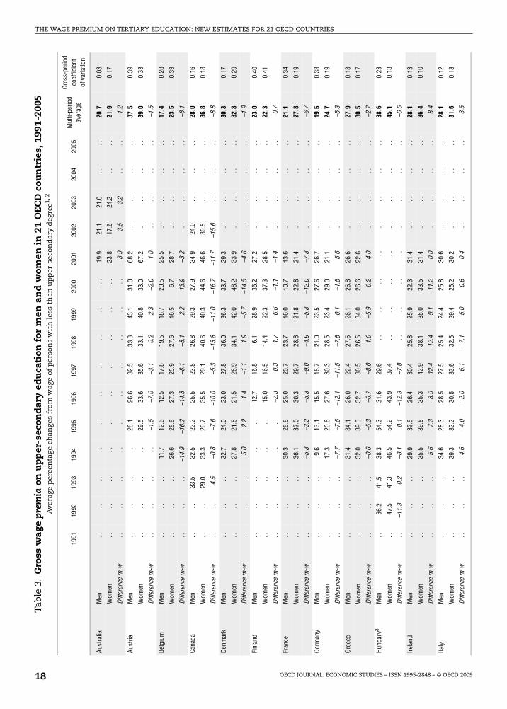
In 2001, not having completed upper-secondary education affected log wages verydifferently, ranging from –0.13 in France to –0.65 in the United States. This implies upper-
secondary wage premia between 14% and 92% of the average wage of persons without
complete upper-secondary education (Table 3). Premia appear to be substantially higher forwomen than for men in Canada and France but lower in the Netherlands and in
Switzerland. Over and above the substantial cross-country variation, upper-secondarywage premia are subject to stronger fluctuations over time. The coefficient of variation
averages 0.20 for the 42 country-gender pairs, which is 1½ times that for tertiary education.Thus persons without completed secondary education appear to be more exposed to
business cycle shocks than lower-educated persons.21
OECD JOURNAL: ECONOMIC STUDIES – ISSN 1995-2848 – © OECD 2009 13

THE WAGE PREMIUM ON TERTIARY EDUCATION: NEW ESTIMATES FOR 21 OECD COUNTRIESTa
ble
2.G
ross
wag
e pr
emia
on
ter
tiar
y ed
uca
tion
for
men
an
d w
omen
in
21
OEC
D c
oun
trie
s, 1
991-
2005
Ave
rage
per
cen
tage
ch
ange
s fr
om w
age
of
up
per
-sec
ond
ary
deg
ree
hol
der
s1,2
1991
1992
1993
1994
1995
1996
1997
1998
1999
2000
2001
2002
2003
2004
2005
Mul
ti-pe
riod
aver
age
Cros
s-pe
riod
coef
ficie
nt
ofva
riatio
n
Men
....
....
....
....
....
42.1
40.6
41.3
....
41.4
0.02
Wom
en..
....
....
....
....
..34
.240
.039
.2..
..37
.80.
08
Diff
eren
ce m
-w..
....
....
....
....
..7.
90.
72.
2..
..3.
6
Men
....
....
63.4
61.7
51.2
54.8
58.9
61.8
53.8
....
....
58.0
0.08
Wom
en..
....
..74
.476
.054
.748
.949
.839
.133
.3..
....
..53
.70.
30
Diff
eren
ce m
-w..
....
..–1
1.0
–14.
3–3
.55.
99.
222
.720
.5..
....
..4.
2
Men
....
..36
.934
.935
.936
.743
.236
.136
.140
.2..
....
..37
.50.
07
Wom
en..
....
24.9
28.8
24.4
30.0
31.4
45.0
34.2
36.3
....
....
31.9
0.21
Diff
eren
ce m
-w..
....
12.0
6.1
11.6
6.7
11.8
–8.8
1.9
3.8
....
....
5.6
Men
....
27.7
26.3
29.3
40.2
31.3
38.9
38.7
51.9
49.5
47.1
....
..38
.10.
24
Wom
en..
..39
.337
.634
.441
.436
.843
.342
.858
.755
.455
.2..
....
44.5
0.20
Diff
eren
ce m
-w..
..–1
1.6
–11.
3–5
.1–1
.2–5
.4–4
.4–4
.1–6
.8–5
.8–8
.1..
....
–6.4
Men
....
..24
.131
.630
.231
.238
.539
.840
.547
.6..
....
..35
.40.
21
Wom
en..
....
25.2
29.2
30.8
25.3
38.4
35.9
37.2
42.6
....
....
33.1
0.19
Diff
eren
ce m
-w..
....
–1.1
2.4
–0.6
5.9
0.1
3.8
3.3
5.0
....
....
2.4
Men
....
....
..53
.656
.447
.453
.554
.552
.6..
....
..53
.00.
06
Wom
en..
....
....
39.8
38.2
36.0
41.3
38.9
43.1
....
....
39.5
0.06
Diff
eren
ce m
-w..
....
....
13.8
18.2
11.5
12.2
15.7
9.6
....
....
13.5
Men
....
..67
.965
.566
.370
.372
.664
.871
.158
.8..
....
..67
.20.
07
Wom
en..
....
56.7
55.9
56.4
63.8
63.7
57.7
57.6
57.2
....
....
58.6
0.05
Diff
eren
ce m
-w..
....
11.2
9.6
9.9
6.5
8.9
7.0
13.6
1.6
....
....
8.5
Men
....
..41
.942
.439
.940
.746
.353
.550
.546
.3..
....
..45
.20.
11
Wom
en..
....
35.2
42.8
37.4
41.1
40.8
47.1
42.2
49.6
....
....
42.0
0.11
Diff
eren
ce m
-w..
....
6.8
–0.4
2.5
–0.3
5.5
6.4
8.3
–3.3
....
....
3.2
Men
....
..30
.630
.132
.630
.229
.235
.435
.735
.3..
....
..32
.40.
08
Wom
en..
....
26.6
23.4
27.5
33.4
50.7
45.2
45.5
47.2
....
....
37.4
0.29
Diff
eren
ce m
-w..
....
3.9
6.7
5.1
–3.1
–21.
4–9
.8–9
.8–1
1.9
....
....
–5.0
Men
..66
.258
.661
.241
.155
.561
.1..
....
....
....
..57
.30.
15
Wom
en..
44.1
58.9
66.4
58.4
49.9
59.3
....
....
....
....
56.2
0.14
Diff
eren
ce m
-w..
22.1
–0.4
–5.2
–17.
35.
71.
8..
....
....
....
..1.
1
Men
....
..31
.837
.340
.360
.553
.351
.752
.854
.3..
....
..47
.80.
21
Wom
en..
....
40.5
47.8
51.1
76.0
58.7
71.7
59.6
68.4
....
....
59.2
0.21
Diff
eren
ce m
-w..
....
–8.7
–10.
5–1
0.9
–15.
5–5
.3–2
0.0
–6.8
–14.
1..
....
..–1
1.5
Men
....
..42
.339
.843
.144
.651
.850
.449
.650
.9..
....
..46
.60.
10
Wom
en..
....
39.2
37.5
35.5
35.1
38.3
40.4
43.1
38.8
....
....
38.5
0.07
Diff
eren
ce m
-w..
....
3.1
2.3
7.6
9.5
13.5
10.0
6.4
12.1
....
....
8.1
OECD JOURNAL: ECONOMIC STUDIES – ISSN 1995-2848 – © OECD 200914
Aust
ralia
Aust
ria
Belg
ium
Cana
da
Den
mar
k
Finl
and
Fran
ce
Ger
man
y
Gre
ece
Hun
gary
3
Irel
and
Italy

TRIES
THE WAGE PREMIUM ON TERTIARY EDUCATION: NEW ESTIMATES FOR 21 OECD COUNrg3
Men
....
....
62.7
56.2
51.4
64.5
62.5
67.4
52.6
....
....
59.6
0.10
Wom
en..
....
..67
.651
.750
.459
.053
.856
.449
.3..
....
..55
.50.
11
Diff
eren
ce m
-w..
....
..–4
.94.
50.
95.
58.
611
.13.
3..
....
..4.
1
sM
en..
....
48.9
49.3
48.6
43.0
40.3
33.4
38.5
41.7
....
....
43.0
0.13
Wom
en..
....
36.2
41.0
41.7
32.0
31.1
30.9
30.3
45.9
....
....
36.1
0.17
Diff
eren
ce m
-w..
....
12.6
8.3
6.9
11.0
9.2
2.5
8.2
–4.2
....
....
6.8
Men
....
....
....
40.2
48.5
52.9
35.8
....
....
..44
.40.
18
Wom
en..
....
....
..55
.965
.880
.184
.7..
....
....
71.6
0.18
Diff
eren
ce m
-w..
....
....
..–1
5.7
–17.
2–2
7.1
–48.
9..
....
....
–27.
2
Men
....
..67
.087
.210
4.6
80.2
87.6
75.8
87.0
65.8
....
....
81.9
0.15
Wom
en..
....
68.6
77.1
90.2
77.2
95.7
82.2
113.
691
.8..
....
..87
.10.
16
Diff
eren
ce m
-w..
....
–1.6
10.1
14.4
3.1
–8.1
–6.3
–26.
6–2
6.0
....
....
–5.1
Men
....
..27
.829
.829
.823
.422
.218
.215
.626
.9..
....
..24
.20.
22
Wom
en..
....
34.5
36.8
34.6
29.8
25.2
25.2
25.0
36.5
....
....
31.0
0.17
Diff
eren
ce m
-w..
....
–6.7
–7.0
–4.8
–6.4
–3.0
–7.0
–9.4
–9.6
....
....
–6.7
Men
....
....
....
27.2
32.1
32.9
32.1
29.6
....
....
30.8
0.08
Wom
en..
....
....
..25
.524
.418
.522
.123
.7..
....
..22
.90.
12
Diff
eren
ce m
-w..
....
....
..1.
77.
714
.39.
95.
9..
....
..7.
9
d3M
en..
....
....
....
..50
.746
.0..
....
....
48.4
0.07
Wom
en..
....
....
....
..40
.939
.2..
....
....
40.1
0.03
Diff
eren
ce m
-w..
....
....
....
..9.
86.
8..
....
....
8.3
gdom
Men
69.7
68.5
71.5
69.2
62.8
68.3
65.9
66.4
68.9
64.5
65.2
62.9
58.5
52.1
..65
.30.
08
Wom
en72
.384
.779
.774
.574
.571
.174
.475
.171
.765
.271
.569
.361
.953
.9..
71.4
0.10
Diff
eren
ce m
-w–2
.6–1
6.2
–8.2
–5.2
–11.
6–2
.8–8
.5–8
.7–2
.8–0
.7–6
.3–6
.4–3
.3–1
.8..
–6.1
tes
Men
....
..80
.980
.184
.180
.376
.990
.589
.891
.610
0.8
92.2
95.4
94.6
88.1
0.08
Wom
en..
....
82.6
84.1
87.6
84.9
82.5
89.0
87.9
89.4
94.2
84.0
90.6
89.9
87.2
0.04
Diff
eren
ce m
-w..
....
–1.8
–4.0
–3.6
–4.6
–5.6
1.5
1.9
2.2
6.6
8.2
4.8
4.6
0.9
s “n
ot a
vail
able
”. o
f ch
angi
ng
vari
able
edu
3 fr
om 0
to
1, l
eavi
ng
oth
er v
aria
bles
un
chan
ged
. G
iven
th
e p
oin
t es
tim
ates
for
men
(α 2
) an
d w
omen
(α 2
+α 4
), pr
emia
eq
ual
[ex
p(α
2)–1
]*10
0% a
nd
2+
α 4)–
1]*1
00%
, res
pec
tive
ly.
es o
f th
e u
nd
erly
ing
po
int
esti
mat
es n
ot
rep
ort
ed. A
ll c
oef
fici
ents
fo
r m
en s
ign
ific
ant
at t
he
1% l
evel
. Wag
e pr
emia
fo
r w
omen
are
sig
nif
ican
tly
dif
fere
nt
fro
m z
ero
bu
t n
ot
all
are
ican
tly
dif
fere
nt
fro
m m
ale
wag
e pr
emia
(se
e Fi
gure
4).
atio
n b
ased
on
net
hou
rly
wag
es a
nd
, hen
ce, r
esu
lts
no
t d
irec
tly
com
par
able
wit
h t
hos
e fo
r o
ther
cou
ntr
ies.
uth
ors’
cal
cula
tio
ns.
Tabl
e 2.
Gro
ss w
age
prem
ia o
n t
erti
ary
edu
cati
on f
or m
en a
nd
wom
en i
n 2
1O
ECD
cou
ntr
ies,
199
1-20
05 (
cont
.)A
vera
ge p
erce
nta
ge c
han
ges
from
wag
e o
f u
pp
er-s
econ
dar
y d
egre
e h
old
ers1,
2
1991
1992
1993
1994
1995
1996
1997
1998
1999
2000
2001
2002
2003
2004
2005
Mul
ti-pe
riod
aver
age
Cros
s-pe
riod
coef
ficie
nt
ofva
riatio
n
OECD JOURNAL: ECONOMIC STUDIES – ISSN 1995-2848 – © OECD 2009 15
Luxe
mbo
u
Net
herla
nd
Pola
nd
Portu
gal
Spai
n
Swed
en3
Switz
erla
n
Uni
ted
Kin
Uni
ted
Sta
. .:
Mea
n1.
Effe
ct[e
xp
(α2.
t-va
lusi
gnif
3.Es
tim
Sour
ce:
A

THE WAGE PREMIUM ON TERTIARY EDUCATION: NEW ESTIMATES FOR 21 OECD COUNTRIES
Concerning the variables other than educational attainment, the following points areworth noting with reference to 2001 estimates:22
● Skill accumulation is rewarded throughout but the relative importance of general labour-market relative to job-specific skills varies across countries:
❖ The experience premium ranges from 0.23% per annum in Germany to 1.69% inSwitzerland, appears to be lower for women than for men (except for Poland and
Portugal), and turns out to be fairly stable over time;
❖ the effect of an additional year of job tenure (0.3% to 3.1%) tends to be negatively
correlated with the experience premium;
● The estimated gender pay gap (all education levels) averages 15% in 2001 and is highest
in Poland (36% of the male wage) and lowest in Sweden (5%).
● Married persons tend to earn significantly more than non-married persons in
17 countries (up to 23% in Poland) but not in Belgium, Finland, Hungary and Switzerland.
● Working for the public sector entails positive wage effects in the majority of countries,
with the premium exceeding 20% in Canada, Luxembourg and Portugal, but a penalty inthe Nordic countries and the United States.23
● The wage effect of working part-time is heterogeneous across countries: while positivein the majority of countries (as high as 30% in Greece and Italy), it tends to be negative in
the English-speaking countries (nearly –20% in the United States).
Figure 4. Male-female differences in tertiary-education coefficients90% confidence intervals of point estimates, 20011
1. Except Hungary (1997); and Poland and Swizerland (2000).2. Net wage for Hungary, Luxembourg, Poland, and Switzerland.3. Upper bar: men; lower bar: women.
Source: Authors' calculations.
0 0.10 0.20 0.30 0.40 0.50 0.60 0.70 0.80
Men WomenCountry3
Average premium over gross2 hourly wage of upper-secondary degree holder
Germany
Switzerland
Luxembourg
United Kingdom
Australia
BelgiumCanada
France
Greece
Ireland
United States
Poland
Austria
Denmark
FinlandSpain
Netherlands
Sweden
Hungary
Portugal
Italy
OECD JOURNAL: ECONOMIC STUDIES – ISSN 1995-2848 – © OECD 200916

TRIES
THE WAGE PREMIUM ON TERTIARY EDUCATION: NEW ESTIMATES FOR 21 OECD COUN● An indefinite-term contract improves a worker’s wage by between 6% and 84% on average.
● A person working in a plant twice the size of another person’s plant earns between 2%(Netherlands) and 6% (Germany) more.
● Being over-qualified reduces the hourly pay by between 12% (Switzerland) and 37% (UnitedStates) of the upper-secondary degree holder’s wage whereas being under-qualified raises
wages by 9% to 43% compared with persons with the same attainment level working inlower occupations; the point estimators suggest that on average: i) working in “too low” an
occupation does not fully take away the education wage premium; and ii) making it to “toohigh” an occupation does not fully substitute for education.
Figure 5. Evolution of gross wage premia for selected countries1994-2001
Source: Authors' calculations.
1994 1995 1996 1997 1998 1999 2000 2001
120
100
80
60
40
20
0
1994 1995 1996 1997 1998 1999 2000 2001
120
100
80
60
40
20
0
Per cent of upper-secondary wageMen
Per cent of upper-secondary wageWomen
GreeceDenmark
Portugal
Germany
United Kingdom
Ireland
United States
OECD JOURNAL: ECONOMIC STUDIES – ISSN 1995-2848 – © OECD 2009 17
THE WAGE PREMIUM ON TERTIARY EDUCATION: NEW ESTIMATES FOR 21 OECD COUNTRIESTa
ble
3.G
ross
wag
e pr
emia
on
up
per
-sec
ond
ary
edu
cati
on f
or m
en a
nd
wom
en i
n 2
1O
ECD
cou
ntr
ies,
199
1-20
05A
vera
ge p
erce
nta
ge c
han
ges
from
wag
e of
per
son
s w
ith
less
th
an u
pp
er-s
econ
dar
y d
egre
e1,2
1991
1992
1993
1994
1995
1996
1997
1998
1999
2000
2001
2002
2003
2004
2005
Mul
ti-pe
riod
aver
age
Cros
s-pe
riod
coef
ficie
nt
ofva
riatio
n
Men
....
....
....
....
....
19.9
21.1
21.0
....
20.7
0.03
Wom
en..
....
....
....
....
..23
.817
.624
.2..
..21
.90.
17
Diff
eren
ce m
-w..
....
....
....
....
..–3
.93.
5–3
.2..
..–1
.2
Men
....
....
28.1
26.6
32.5
33.3
43.1
31.0
68.2
....
....
37.5
0.39
Wom
en..
....
..29
.533
.635
.633
.140
.833
.067
.2..
....
..39
.00.
33
Diff
eren
ce m
-w..
....
..–1
.5–7
.0–3
.10.
22.
3–2
.01.
0..
....
..–1
.5
Men
....
..11
.712
.612
.517
.819
.518
.720
.525
.5..
....
..17
.40.
28
Wom
en..
....
26.6
28.8
27.3
25.9
27.6
16.5
6.7
28.7
....
....
23.5
0.33
Diff
eren
ce m
-w..
....
–14.
9–1
6.2
–14.
8–8
.1–8
.12.
213
.9–3
.2..
....
..–6
.1
Men
....
33.5
32.5
22.2
25.5
23.8
26.8
29.3
27.9
34.9
24.0
....
..28
.00.
16
Wom
en..
..29
.033
.329
.735
.529
.140
.640
.344
.646
.639
.5..
....
36.8
0.18
Diff
eren
ce m
-w..
..4.
5–0
.8–7
.6–1
0.0
–5.3
–13.
8–1
1.0
–16.
7–1
1.7
–15.
6..
....
–8.8
Men
....
..32
.724
.023
.027
.836
.036
.333
.729
.3..
....
..30
.30.
17
Wom
en..
....
27.8
21.8
21.5
28.9
34.1
42.0
48.2
33.9
....
....
32.3
0.29
Diff
eren
ce m
-w..
....
5.0
2.2
1.4
–1.1
1.9
–5.7
–14.
5–4
.6..
....
..–1
.9
Men
....
....
..12
.716
.816
.128
.936
.227
.2..
....
..23
.00.
40
Wom
en..
....
....
15.0
16.5
14.4
22.3
37.3
28.5
....
....
22.3
0.41
Diff
eren
ce m
-w..
....
....
–2.3
0.3
1.7
6.6
–1.1
–1.4
....
....
0.7
Men
....
..30
.328
.825
.020
.723
.716
.010
.713
.6..
....
..21
.10.
34
Wom
en..
....
36.1
32.0
30.3
29.7
28.6
21.8
22.8
21.4
....
....
27.8
0.19
Diff
eren
ce m
-w..
....
–5.8
–3.2
–5.3
–9.0
–4.9
–5.8
–12.
0–7
.8..
....
..–6
.7
Men
....
..9.
613
.115
.518
.721
.023
.527
.626
.7..
....
..19
.50.
33
Wom
en..
....
17.3
20.6
27.6
30.3
28.5
23.4
29.0
21.1
....
....
24.7
0.19
Diff
eren
ce m
-w..
....
–7.7
–7.5
–12.
1–1
1.5
–7.5
0.1
–1.5
5.6
....
....
–5.3
Men
....
..31
.434
.126
.022
.427
.528
.126
.826
.6..
....
..27
.90.
13
Wom
en..
....
32.0
39.3
32.7
30.5
26.5
34.0
26.6
22.6
....
....
30.5
0.17
Diff
eren
ce m
-w..
....
–0.6
–5.3
–6.7
–8.0
1.0
–5.9
0.2
4.0
....
....
–2.7
Men
..36
.241
.538
.354
.331
.629
.6..
....
....
....
..38
.60.
23
Wom
en..
47.5
41.3
46.5
54.2
43.9
37.4
....
....
....
....
45.1
0.13
Diff
eren
ce m
-w..
–11.
30.
2–8
.10.
1–1
2.3
–7.8
....
....
....
....
–6.5
Men
....
..29
.932
.526
.430
.425
.825
.922
.331
.4..
....
..28
.10.
13
Wom
en..
....
35.5
39.8
35.3
42.9
38.1
35.0
33.5
31.4
....
....
36.4
0.10
Diff
eren
ce m
-w..
....
–5.6
–7.3
–8.9
–12.
4–1
2.4
–9.1
–11.
20.
0..
....
..–8
.4
Men
....
..34
.628
.328
.527
.525
.424
.425
.830
.6..
....
..28
.10.
12
Wom
en..
....
39.3
32.2
30.5
33.6
32.5
29.4
25.2
30.2
....
....
31.6
0.13
Diff
eren
ce m
-w..
....
–4.6
–4.0
–2.0
–6.1
–7.1
–5.0
0.6
0.4
....
....
–3.5
OECD JOURNAL: ECONOMIC STUDIES – ISSN 1995-2848 – © OECD 200918
Aust
ralia
Aust
ria
Belg
ium
Cana
da
Den
mar
k
Finl
and
Fran
ce
Ger
man
y
Gre
ece
Hun
gary
3
Irel
and
Italy

THE WAGE PREMIUM ON TERTIARY EDUCATION: NEW ESTIMATES FOR 21 OECD COUNTRIES
rg3
Men
....
....
66.4
50.6
49.4
43.7
50.0
52.0
52.3
....
....
52.1
0.13
Wom
en..
....
..72
.668
.752
.239
.147
.957
.650
.4..
....
..55
.50.
21
Diff
eren
ce m
-w..
....
..–6
.2–1
8.1
–2.8
4.6
2.1
–5.6
1.9
....
....
–3.4
sM
en..
....
40.4
29.0
33.1
29.9
28.2
24.3
26.0
30.1
....
....
30.1
0.16
Wom
en..
....
38.0
32.1
28.1
30.2
24.4
21.7
21.2
17.4
....
....
26.7
0.25
Diff
eren
ce m
-w..
....
2.4
–3.1
5.0
–0.3
3.8
2.6
4.8
12.7
....
....
3.5
Men
....
....
....
35.0
31.2
36.1
34.1
....
....
..34
.10.
06
Wom
en..
....
....
..30
.730
.134
.335
.3..
....
....
32.6
0.08
Diff
eren
ce m
-w..
....
....
..4.
41.
11.
7–1
.2..
....
....
1.5
Men
....
..77
.874
.861
.372
.641
.954
.744
.855
.9..
....
..60
.50.
23
Wom
en..
....
98.5
92.8
86.0
84.7
53.3
59.0
48.2
57.8
....
....
72.5
0.27
Diff
eren
ce m
-w..
....
–20.
7–1
8.0
–24.
8–1
2.1
–11.
5–4
.3–3
.4–1
.8..
....
..–1
2.1
Men
....
..42
.843
.945
.649
.349
.542
.341
.431
.4..
....
..43
.30.
13
Wom
en..
....
47.3
47.4
39.9
47.3
50.2
45.5
40.6
28.6
....
....
43.3
0.16
Diff
eren
ce m
-w..
....
–4.5
–3.5
5.7
2.1
–0.7
–3.2
0.8
2.8
....
....
–0.1
Men
....
....
....
14.3
14.8
16.5
20.0
19.3
....
....
17.0
0.15
Wom
en..
....
....
..11
.38.
814
.78.
913
.3..
....
..11
.40.
23
Diff
eren
ce m
-w..
....
....
..3.
05.
91.
811
.16.
0..
....
..5.
6
d3M
en..
....
....
....
..10
6.7
85.2
....
....
..96
.00.
16
Wom
en..
....
....
....
..71
.646
.3..
....
....
58.9
0.30
Diff
eren
ce m
-w..
....
....
....
..35
.138
.9..
....
....
37.0
gdom
Men
32.2
48.9
49.4
56.7
47.8
52.5
47.8
43.5
44.7
45.9
42.0
39.5
43.5
43.4
..45
.60.
13
Wom
en38
.847
.353
.155
.253
.056
.147
.646
.345
.242
.439
.341
.142
.243
.7..
46.5
0.13
Diff
eren
ce m
-w–6
.61.
6–3
.61.
5–5
.2–3
.50.
2–2
.9–0
.53.
42.
7–1
.61.
3–0
.3..
–1.0
tes
Men
....
..95
.990
.185
.695
.286
.792
.594
.891
.589
.982
.185
.584
.189
.50.
05
Wom
en..
....
82.8
88.9
78.2
83.7
87.8
83.4
92.2
92.3
91.1
76.3
79.1
82.8
84.9
0.07
Diff
eren
ce m
-w..
....
13.1
1.2
7.4
11.5
–1.1
9.2
2.6
–0.9
–1.2
5.8
6.4
1.4
4.6
s “n
ot a
vail
able
”. o
f ch
angi
ng
vari
able
edu
1fr
om 0
to 1
, le
avin
g o
ther
var
iabl
es u
nch
ange
d.
As
the
Min
cer
equ
atio
ns
use
th
e av
erag
e u
pp
er-s
econ
dar
y d
egre
e h
old
er a
s th
e re
fere
nce
per
son
, th
isre
s tr
ansf
orm
ing
the
init
ial
(neg
ativ
e) M
ince
r co
effi
cien
t fo
r m
en,
α 1, i
nto
[1/
exp
(α1)
–1]*
100%
an
d t
hat
for
wom
en, (
α 1+
α 3),
into
[1/
exp
(α1
+α 3
)–1]
*100
%. E
xam
ple
: α 1
=–0
.30
wou
ldla
te i
nto
an
up
per
-sec
on
dar
y w
age
pre
miu
m o
f 35
% a
s [1
/exp
(–0.
30)]
–1=
0.35
.es
of
the
un
der
lyin
g p
oin
t es
tim
ates
not
rep
orte
d.
All
co
effi
cien
ts f
or
men
are
sig
nif
ican
t at
th
e 1%
lev
el e
xce
pt
for
Bel
giu
m i
n20
00 (
5% l
evel
). W
age
prem
ia f
or
wom
en a
re a
lso
ican
tly
dif
fere
nt
fro
m z
ero
bu
t n
ot a
ll o
f th
em a
re s
ign
ific
antl
y d
iffe
ren
t fr
om m
ale
prem
ia.
atio
n b
ased
on
net
ho
url
y w
ages
an
d, h
ence
, res
ult
s n
ot
dir
ectl
y co
mp
arab
le w
ith
th
ose
for
oth
er c
oun
trie
s.
uth
ors'
cal
cula
tio
ns.
Tabl
e 3.
Gro
ss w
age
prem
ia o
n u
pp
er-s
econ
dar
y ed
uca
tion
for
men
an
d w
omen
in
21
OEC
D c
oun
trie
s, 1
991-
2005
(co
nt.)
Ave
rage
per
cen
tage
ch
ange
s fr
om w
age
of p
erso
ns
wit
h le
ss t
han
up
per
-sec
ond
ary
deg
ree1,
2
1991
1992
1993
1994
1995
1996
1997
1998
1999
2000
2001
2002
2003
2004
2005
Mul
ti-pe
riod
aver
age
Cros
s-pe
riod
coef
ficie
nt
ofva
riatio
n
OECD JOURNAL: ECONOMIC STUDIES – ISSN 1995-2848 – © OECD 2009 19
Luxe
mbo
u
Net
herla
nd
Pola
nd
Portu
gal
Spai
n
Swed
en3
Switz
erla
n
Uni
ted
Kin
Uni
ted
Sta
. .:
Mea
n1.
Effe
ctre
qu
itr
ans
2.t-
valu
sign
if3.
Esti
mSo
urce
:A

THE WAGE PREMIUM ON TERTIARY EDUCATION: NEW ESTIMATES FOR 21 OECD COUNTRIES
The gross hourly wage premium per annum of tertiary education
Two adjustments are made for the results to be fully comparable across countries.
First, a correction is required to assess the gross wage premium for the four countries forwhich only net wages are available. Second, all gross wage premia upon completion of
tertiary education are transformed into wage premia per annum of tertiary education toaccount for cross-country differences in the duration of tertiary studies.
The correction of net attainment premia follows de la Fuente and Jimeno (2005). Theaverage income tax rate t of the average earner in 2001 is taken from OECD (2005a).24 It
equals 33.3% for Hungary, 27.8% for Luxembourg, 32.4% for Sweden, and 22% for Switzerland.The precise wage premia derived from the estimated edu3 coefficients in the log net wage
equations are divided by (1 – t) to obtain gross tertiary wage premia. This brings Hungary tothe top of the country ranking. Moreover, Sweden is no longer at the bottom.
To express the results as gross wage premia per annum of tertiary education, thecountry-specific average tertiary study duration d is taken from Table B1.3b of OECD
(2005b) and applied to the wage premia reported in Table 2.25 This is done by taking
(1 + wage premium) to the power of (1/d), i.e. assuming a constant percentage increase inthe hourly wage for each year of tertiary education. Figure 6 summarises the results
for 2001, illustrating both the attainment-specific wage premia and the wage premia per
annum of tertiary education. The latter enter the calculation of the private internal rates of
return to tertiary education in Boarini and Strauss (2009).
The country average of the gross hourly wage premium per annum is 10.6% for men and
11% for women. At 10% for each gender, the median is lower than the average, implyingthat the majority of countries is below the average. The median countries are Finland
(men) and France (women). Wage premia are comprised between 5½% to 6% (men in Greeceand Spain, women in Austria and Italy) and 16% to 18% in Hungary and the United States
(both men and women) and for women in Ireland and Portugal. Women in Poland and theUnited Kingdom come close to these top premia.
Intermediate values of gross hourly wage premia per annum of tertiary education areobserved for the majority of countries. For male wage premia, countries fall into three
groups. The first with premia distinctly lower than the median includes Austria, Belgium,Germany, Italy, the Netherlands, Poland and Sweden. The second has premia at 10%
(Canada, Denmark, Finland and France). The remaining countries (third group) outperformboth the median and the average. For women, intermediate premia fall into two country
groups, one with median or higher wage premia (Australia, Canada, France, Luxembourgand Switzerland), the other with premia from 7% to 9%.
Controlling for the duration of tertiary studies significantly changes the position ofsome countries. Australia and Ireland, where studies tend to be shorter than the OECD
average, are now among those with the highest premia. Switzerland and the United Kingdomalso improve their relative position. At the same time, countries characterised by long study
duration such as Austria, Germany, Greece and Italy, fall behind. The same is true, albeit to alesser extent, for France and the Netherlands where the average study duration is about half
a year longer than the OECD average. The negative Pearson rank correlation between studyduration and the wage premium per annum of tertiary education at –0.70 for men and –0.65
for women suggests decreasing returns to additional years of tertiary education beyond the
OECD JOURNAL: ECONOMIC STUDIES – ISSN 1995-2848 – © OECD 200920
first higher-education degree. Countries with long average study duration even fail to
produce higher tertiary attainment premia (not controlling for duration) than those with

TRIES
THE WAGE PREMIUM ON TERTIARY EDUCATION: NEW ESTIMATES FOR 21 OECD COUNshorter programmes, with the coefficient of rank correlation between the 2001 tertiaryattainment premia (see Table 2) and study duration being insignificant at best (–0.20 for men
and –0.26 for women). These results imply that countries with long study duration may havescope for strengthening the overall incentive to invest in tertiary human capital through
curricular reform, e.g. by streamlining and better co-ordinating study programmes, reducing
Figure 6. Gross wage premia20011
1. Except Hungary (1997); and Poland and Swizerland (2000).2. The total wage premium associated with a tertiary education level is converted to an annual basis by taking into
account the duration of tertiary studies.
Source: Authors' calculations.
100 18
16
14
12
10
8
6
4
2
0
90
80
70
60
50
40
30
20
10
0
100 18
16
14
12
10
8
6
4
2
0
90
80
70
60
50
40
30
20
10
0
Per cent of upper-secondary wageMen
Gross wage premium (left scale)
Gross wage premium per year of tertiary education (right scale)2
German
y
Switzerl
and
Luxe
mbourg
United
Kingdo
m
Austra
lia
Belgium
Franc
e
Greece
Irelan
d
United
States
Poland
Austri
a
Denmark
Finlan
d
Canad
aSpa
in
Netherl
ands
Sweden
Hunga
ry
Portug
alIta
ly
Per cent of upper-secondary wageWomen
German
y
Switzerl
and
Luxe
mbourg
United
Kingdo
m
Austra
lia
Belgium
Franc
e
Greece
Irelan
d
United
States
Poland
Austri
a
Denmark
Finlan
d
Canad
aSpa
in
Netherl
ands
Sweden
Hunga
ry
Portug
alIta
ly
OECD JOURNAL: ECONOMIC STUDIES – ISSN 1995-2848 – © OECD 2009 21
slack in student timetables, and strengthening incentives for studying faster.
THE WAGE PREMIUM ON TERTIARY EDUCATION: NEW ESTIMATES FOR 21 OECD COUNTRIES
Comparison with other estimates in the literature
Given the vast amount of country-specific empirical studies, the focus here is on a
limited number of empirical studies, which like this study have attempted to yieldcomparable results across countries through the use of cross-country data sources and a
unified framework of sample selection and econometric specification.26 Despite thesimilarities the comparability across studies is limited by differences in time and country
coverage, data sources and methods. Bearing this caveat in mind, the following comparisonssuggest that the results of this study are broadly in line with those from earlier studies.
Psacharopoulos (1994) and Psacharopoulos and Patrinos (2004) have the broadestcountry coverage. Where they present university-specific results these pertain to returns to
education rather than wage premia and mostly refer to sample periods prior to thosecovered in this study. However, they also present results from traditional Mincerian wage
equations that include years of schooling (all levels) and labour market experience. Theschooling coefficients average 0.072 for the 16 countries for which the year reported
(early 1990s to mid-1990s, see Table A2 in Psacharopoulos and Patrinos, 2004) is not too far
from the results reported here, compared with 0.100 in this study (gender-country averageof edu3 coefficients of 1996 or closest available year, divided by 4.21 years, the OECD
average duration of tertiary studies).
The Mincerian years-of-schooling coefficients (all educational levels) based on data of
the mid-1990s collected in Asplund and Pereira (1999) and also reported in Harmon et al.
(2003, Table 2) average 0.075 for men and 0.083 for women (specification using potential
experience) for the 14 countries that their samples and those of this study have incommon. This compares with a somewhat higher 0.087 in this study (gender-country
average of edu3 coefficients of 1996 or closest available year, divided by 4.6 years, theaverage study duration in the relevant country group).
Blöndal et al. (2002) compute private internal rates of return to tertiary education at theend of the 1990s for ten countries, eight of which are also in the country sample reported
here. Methodologically, their “narrow rate” comes closest to the wage premium per annum
of tertiary education reported in Figure 6. The average gross wage premium per annum of
education in this group is 11.9% for men and 11% for women and compares to the 2001average premium of 10.5% for each gender in this study. The results are relatively close to
each other given marked differences in data sources, available control variables andmethodology (annual rather than hourly earnings; returns not estimated through
regressions but taken from aggregate data on average gender-age-specific earnings oftertiary- and upper-secondary degree holders).
De la Fuente and Jimeno (2005) use data from labour-force surveys, a quadraticspecification of potential experience and a smaller set of control variables than this study.
Their uncorrected27 OLS estimate for the EU15 countries averages 0.08, comparable withthe 2001 estimate of 0.085 presented here (gender-country average of edu3 coefficients,
divided by the average study duration of 4.7 years). Correlation analysis confirms that thenew results presented in this study are broadly in line with comparable cross-country
studies in the earlier literature. Based on the same sample of countries and using the samereported year (or its closest neighbours) for each cross-study comparison, the correlation
coefficients between our tertiary wage premia and other studies are 0.91 with respect to
OECD JOURNAL: ECONOMIC STUDIES – ISSN 1995-2848 – © OECD 200922
Blöndal et al. (2002); 0.70 with respect to Asplund and Pereira (1999); 0.6 with respect to
TRIES
THE WAGE PREMIUM ON TERTIARY EDUCATION: NEW ESTIMATES FOR 21 OECD COUNPsacharopoulos and Patrinos (2004). Finally, the correlation coefficient between our Mincercoefficients and those reported in the Handbook of the Economics of Education (Peracchi, 2006)
amounts to 0.68.
ConclusionThe gross hourly wage premium is the single most important driver of private returns
to tertiary education. This study has presented cross-section estimations based on aunified framework for 21 OECD countries from the 1990s to the early 2000s using
international (and a few national) household surveys to maximise internationalcomparability. One of the main advantages of the estimates presented here have been the
use of a richer set of control variables and the extension of a single framework to a largernumber of OECD countries than had usually been the case. The results of the “augmented”
Mincerian wage equations point to an average gross hourly wage premium on completedtertiary education of 55% in 2001 (country-gender average), translating into a premium of
almost 11% per annum of tertiary education. Wage premia display little variation over timebut huge cross-country variation, ranging from 27% for men in Spain to 90% for Hungary
and the United States. At 6 %, the premium per annum of tertiary education is lowest inGreece and Spain while reaching 14%-18% in most Anglo-Saxon countries as well as in
Portugal and Hungary.
As discussed in Oliveira Martins et al. (2009, in this issue), it is remarkable that wage
premia have held up well and even tended to increase over time despite the ongoingexpansion of tertiary education. This indicates that the demand for high-skilled workers
has increased at least as much as their supply. The assessment of wage premia on tertiaryeducation should be based on whether they are conducive to the right skill mix in the
economy. Very low wage premia are either indicative of low quality of tertiary education orinsufficient wage differentiation, leading to low demand for tertiary education and under-
provision of skills. But very high wage premia are not all good either since they may reflectan inability of the education system to provide graduates despite strong signals from the
labour markets.
Finally, it should be borne in mind that the financial return expressed in the wage
premia presented in this study are not the only benefits attached to higher education. Asstated in the Stiglitz commission report, education is one of the great pillars of well-being.
It matters not only for financial returns but also for the quality of life. Even though clearcausality is difficult to establish, “better-educated people typically have better health
status, lower unemployment, more social connections, and greater engagement in civicand political life” (Stiglitz Commission, 2009, p. 46).
Notes
1. See Sianesi and Van Reenen (2003) for a survey of empirical studies on macroeconomic returns toeducation.
2. The other large area of policymaking in this respect is university access policies: individuals maybe constrained either by a lack of necessary educational credentials (e.g. in countries rationingaccess to upper-secondary attainment) or by a lack of liquidity. See Oliveira Martins et al. (2009) fora joint empirical analysis of demand and supply-side determinants of investment in tertiaryeducation and how policies affect them.
OECD JOURNAL: ECONOMIC STUDIES – ISSN 1995-2848 – © OECD 2009 23
3. See Psacharopoulos and Patrinos (2004) for a survey of the empirical literature on Mincer equations.

THE WAGE PREMIUM ON TERTIARY EDUCATION: NEW ESTIMATES FOR 21 OECD COUNTRIES
4. For more details see Heckman et al. (2005) where these two interpretations of the Mincerspecification are discussed as the “Compensating Differences Model” and the “Accounting-Identity Model”.
5. In the presence of measurement error, instrumenting the missing ability variable with familybackground is likely to aggravate the measurement error bias (Mellander and Sandgren Massih, 2008).
6. The size of this general-equilibrium effect is somewhat controversial. While Heckman et al. (1999)find the graduate-wage-depressing labour-supply effect of graduation to be large enough to undodiscounted net lifetime income gains, Lee (2005) finds an only mild reduction in these gains fromthe labour-supply effect.
7. The correlation coefficient between attainment and obtaining an indefinite-term contract issignificant only in about half the countries and is rarely larger than 0.10. Attainment is moresystematically correlated with working in the public sector, with the correlation coefficientaveraging some 0.2. Finally, the correlation between attainment and firm size is fairly systematic,too, albeit less strong (coefficient of 0.11 on average). A careful country-by-country tabulation of allbilateral correlations among independent variables can be found in the working paper version ofthis study (Strauss and de la Maisonneuve, 2007).
8. For an in-depth description of the data sources, data issues and the construction of variables seeStrauss and de la Maisonneuve (2007).
9. What matters for the return to tertiary education is the additional net wage at tertiary levelcompared with that at upper-secondary level. This requires the marginal income tax rate of anupper-secondary degree holder to be applied on the gross wage premium (Boarini and Strauss, 2009).
10. As the intention is to use wage premia of today’s workers to gauge the profitability of tertiaryeducation for today’s students contingent on normal labour market participation, droppingworkers with less than 15 hours per week is appropriate based on the assumption that theirdecision to work few hours is voluntary.
11. For France and the Netherlands the attainment variable is corrected for errors in the raw data (seeStrauss and de la Maisonneuve, 2007).
12. Returns to tertiary education depend not only on study completion but also on the type of degreeand the field of study (e.g. see Borland 2002 and Stark 2006 on empirical results for Australia andCanada, respectively). However, information on study fields is missing in most of the datasetsanalysed here.
13. Only for Australia is the actual number of years worked directly available. For all other countriesthere is some deviation from the actual labour market experience. The error is expected to besmall for men but larger for women. Thus it is expected that the female experience premium fallsshort of its male counterpart.
14. F-tests conclude that the joint hypothesis of the effects of all control variables jointly being thesame for men as for women is rejected for each country. However, the subset of variablesresponsible for the rejection varies from country to country.
15. For example, persons in the ECHP whose answer corresponds to the plant-size class“between 20 and 49 persons” are randomly assigned an integer value from 20 to 49.
16. Dumont (2005) discusses the pros and cons of alternative assessment methods for over-qualification.
17. While the margin of 10% is arbitrary, not correcting at all does not seem useful either since simplytaking the mode of the attainment distribution would lead to implausibly high shares ofoccupation-attainment mismatches.
18. Since educational requirements tend to increase over time, many older workers may appear to beunder-qualified according to the simple metric used here but they compensate for this by longerexperience in their jobs or on the labour market more generally. There is indeed positivecorrelation between experience and underqualif in the data, potentially reducing the impact of theexperience variable. Conversely, the correlation between exper and overqualif is negative asexpected – most overqualified persons tend to be young – but the correlation coefficient is muchsmaller in absolute terms and not significant for a number of countries.
19. However, estimations for Sweden are based on net wages. When correcting for the income taxes,the wage premium is lowest in Austria at 33%.
OECD JOURNAL: ECONOMIC STUDIES – ISSN 1995-2848 – © OECD 200924
20. Exceptions to this rule with respect to the wage effect of tertiary education include women inAustria (much lower premia in 2000 and 2001 than before), Belgium (one-off jump in 1999), Greece
TRIES
THE WAGE PREMIUM ON TERTIARY EDUCATION: NEW ESTIMATES FOR 21 OECD COUN(one-off jump in 1998), Ireland (jump in 1997), Luxembourg (1995 premium much higher than forall other years), Portugal (one-off jump in 2000). Results for men are very stable apart from dropsin premia in 2001 for both Poland and Portugal. A sudden increase of about 15 percentage points isobserved for both genders in Canada in 2000.
21. That said, labour market institutions such as minimum wages and collective bargainingagreements shield lower-skilled persons to some extent from large swings in wage premia.However, the cyclical vulnerability of the low-skilled shows very clearly in the employmentprobability (see Boarini and Strauss, 2009, in this issue).
22. The precise wage effect of a 0-1 change in any dummy variable reported in this paragraph isobtained in the same way as the wage effect of completing tertiary education.
23. The interpretation of this result is that employees of the public sector do not appear to “pay theprice” for their much higher job security in most European countries, at least until 2001.
24. Admittedly, correcting with the same average tax rate for all individuals is a rough correction. Tothe extent that persons with higher incomes have higher average tax rates than persons withlower income, the gross premia obtained in this way might slightly understate the true wage premia.
25. Missing study-duration data for six countries (Belgium, Canada, Luxembourg, Poland, Portugal,and the United States) are replaced with the simple OECD country mean (4.21 years). For sixcountries, study duration refers to the year 2001/02, for the others to 1994/95.
26. Country-specific studies can exploit different micro data sources that are not necessarilycomparable with the survey data used in this study. A case in point is Ciccone et al. (2004) whoreport a net hourly wage premium of 9% for Italy, in contrast with the 7% for the gross wagepremium reported in this study.
27. The final gross wage premia per annum of education in de la Fuente and Jimeno (2005) contain anad hoc correction factor of 0.9 accounting for the likely net endogeneity bias (see Card, 1999).
Bibliography
Asplund, R. and P. Pereira (1999), “Returns to Education in Europe: A Literature Review”, ETLA (TheResearch Institute of the Finnish Economy), Taloustieto Oy.
Becker, G.S. (1964), “Human Capital: A Theoretical and Empirical Analysis, With Special Reference toEducation”, Columbia University Press, New York.
Ben-Porath, Y. (1967), “The Production of Human Capital and the Life-Cycle of Earnings”, Journal ofPolitical Economy, 75 (4, Part 1), pp. 352-365.
Birch, A., A. Haag, S. Lefebure, A. Villeret, and G. Schmaus, under support of K. Fischer, J. Frick,B. Kuchler and N. Hegerle (2003), “User Guide”, CHER Working Paper 2, CEPS/INSTEAD, Differdange(G.D. Luxembourg).
Blöndal, S., S. Field and N. Girouard (2002), “Investment in Human Capital Through Upper-Secondaryand Tertiary Education”, OECD Economics Studies, 34 (1), pp. 41-90.
Boarini, R. and H. Strauss (2009), “The Private Internal Rates of Return to Tertiary Education: NewEstimates for 21 OECD Countries”, OECD Journal: Economic Studies, Vol. 2009 (in this issue).
Borland, J. (2002), “New Estimates of the Private Return to University Education in Australia”,Melbourne Institute Working Paper No. 14/02.
Card, D. (1999), “The Causal Effects of Education on Earnings”, in: O. Ashenfelter, and D. Card (eds.),“Handbook of Labour Economics”, Vol. 3, Elsevier.
Ciccone, A., F. Cingano and P. Cipollone (2004), “The Private and Social Return to Schooling in Italy”,Giornale degli Economisti e Annali di Economia, 63 (3-4), pp. 413-444.
De la Fuente, A. and J.F. Jimeno (2005), “The Private and Fiscal Returns to Schooling and the Effect ofPublic Policies on Private Incentives to Invest in Education: A General Framework and Some Resultsfor the EU”, CESifo Working Paper, No. 1392.
Dumont, J.C. (2005), “Level of Education of Immigrants and the Labour Market: Estimating thePrevalence of Overeducation”, OECD Committee on Employment, Labour and Social Affairs,DELSA/ELSA(2005)12, Paris.
OECD JOURNAL: ECONOMIC STUDIES – ISSN 1995-2848 – © OECD 2009 25
Eurostat (2003), “ECHP UDB Description of Variables: Data Dictionary, Codebook and DifferencesBetween Countries and Waves”, Doc. PAN 166/2003-06, Eurostat, Luxembourg.

THE WAGE PREMIUM ON TERTIARY EDUCATION: NEW ESTIMATES FOR 21 OECD COUNTRIES
Harmon, C., H. Oosterbeek and I. Walker (2003), “The Returns to Education: Microeconomics”, Journalof Economic Surveys, 17(2), pp. 115-155.
Heckman, J. (1979), “Sample Selection Bias as a Specification Error”, Econometrica, 47, pp. 153-161.
Heckman, J. (1980), “Sample Selection Bias as a Specification Error with an Application to theEstimation of Labour Supply Functions”, in J.P. Smith (ed.), Female Labour Supply: Theory andEstimation, Princeton University Press, Princeton NJ, pp. 206-248.
Heckman, J., L. Lochner and C. Taber (1999), “General Equilibrium Cost Benefit Analysis of Educationand Tax Policies”, in G. Ranis and L.K. Raut (eds.), Trade, Growth and Development: Essays in Honor ofProfessor T.N. Srinivasan, Elsevier, Amsterdam.
Heckman, J.J., L.J. Lochner and P.E. Todd (2005), “Earnings Functions, Rates of Return, and TreatmentEffects: The Mincer Equation and Beyond”, NBER Working Paper, No. 11544, National Bureau ofEconomic Research.
Hoffmann, R. and A.L. Kassouf (2005), “Deriving Conditional and Unconditional Marginal Effects in LogEarnings Equations Estimated by Heckman’s Procedure”, Applied Economics, 37, pp. 1303-1311.
Lee, D. (2005), “An Estimable Dynamic General Equilibrium Modelof Work, Schooling, andOccupational Choice”, International Economic Review, 46 (1), pp. 1-34.
Mellander, E and S. Sandgren-Massih (2008), “Proxying Abilty by Family Background in Returns toSchooling Estimations is Generally a Bad Idea”, Scandinavian Journal of Economics, 110 (4), pp. 853-875.
Mincer, J. (1958), “Investment in Human Capital and Personal Income Distribution”, Journal of PoliticalEconomy, 66 (4), pp. 281-302.
Mincer, J. (1974), “Schooling, Experience and Earnings”, National Bureau of Economic Research, New York.
OECD (2004), OECD Handbook for Internationally Comparative Education Statistics: Concepts, Standards,Definitions and Classifications, Paris.
OECD (2005a), Taxing Wages, Paris.
OECD (2005b), Education at a Glance, Paris.
Oliveira Martins, J., R. Boarini, H. Strauss and C. de la Maisonneuve (2009), “The Policy Determinants ofInvestment in Tertiary Education”, OECD Journal: Economic Studies, Volume 2009 (in this issue).
Peracchi (2006), “Educational Wage Premia and the Distribution of Earnings: An InternationalPerspective”, in Erik Hanushek and F. Welch (ed.), Handbook of the Economics of Education, Elsevier,Edition 1, Vol. 1, pp. 189-254.
Psacharopoulos, G. (1994), “Returns to Investment in Education: A Global Update”, World Development,22 (9), pp. 1325-1343.
Psacharopoulos, G. and H.A. Patrinos (2004), “Returns to Investment in Education: A Further Update”,Education Economics, 12 (2).
Sianesi, B. and J. Van Reenen (2003), “The Returns to Education: Macroeconomics”, Journal of EconomicSurveys, 17 (2), pp. 157-200.
Stark, A. (2006), “Which Fields Pay, Which Fields Don’t? An Examination of the Returns to UniversityEducation in Canada by Detailed Field of Study”, Economic Analysis and Policy Division,Department of Finance, Canada.
Stiglitz Commission (Commission on the Measurement of Economic Well-being and Social Progress)(2009), Report of Commission on the Measurement of Economic Well-being and Social Progress,Paris, www.stiglitz-sen-fitoussi.fr/documents/rapport_anglais.pdf.
Strauss, H. and de la Maisonneuve (2007), “The Wage Premium on Tertiary Education: New Estimatesfor 21 OECD Countries”, OECD Economics Department Working Paper, No. 589.
Watson, N. (2005), “HILDA User Manual – Release 3.0”, Melbourne Institute of Applied Economic andSocial Research, University of Melbourne.
Woessmann, L. (2003), “Book Review Essay: Returns to Education in Europe”, Review of World Economics,139 (2), pp. 348-376.
OECD JOURNAL: ECONOMIC STUDIES – ISSN 1995-2848 – © OECD 200926
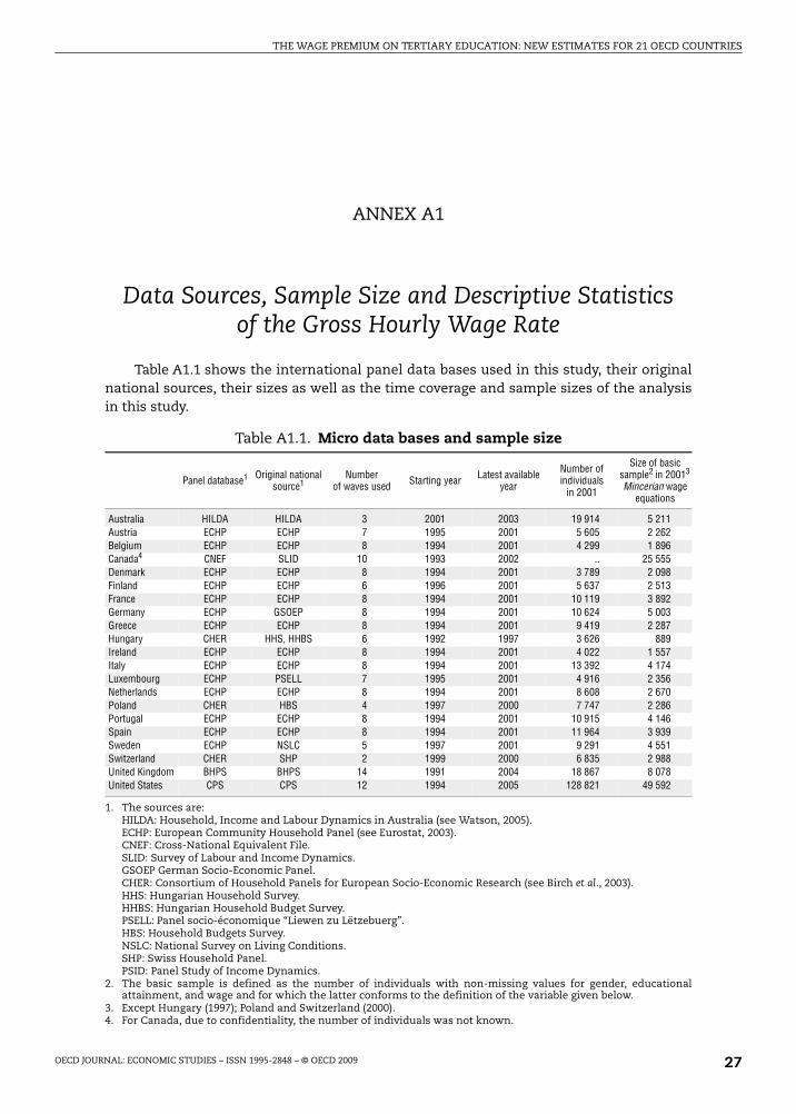
THE WAGE PREMIUM ON TERTIARY EDUCATION: NEW ESTIMATES FOR 21 OECD COUNTRIES
ANNEX A1
Data Sources, Sample Size and Descriptive Statistics of the Gross Hourly Wage Rate
Table A1.1 shows the international panel data bases used in this study, their originalnational sources, their sizes as well as the time coverage and sample sizes of the analysisin this study.
Table A1.1. Micro data bases and sample size
Panel database1 Original national source1
Number of waves used Starting year Latest available
year
Number of individuals
in 2001
Size of basic sample2 in 20013 Mincerian wage
equations
Australia HILDA HILDA 3 2001 2003 19 914 5 211Austria ECHP ECHP 7 1995 2001 5 605 2 262Belgium ECHP ECHP 8 1994 2001 4 299 1 896Canada4 CNEF SLID 10 1993 2002 .. 25 555Denmark ECHP ECHP 8 1994 2001 3 789 2 098Finland ECHP ECHP 6 1996 2001 5 637 2 513France ECHP ECHP 8 1994 2001 10 119 3 892Germany ECHP GSOEP 8 1994 2001 10 624 5 003Greece ECHP ECHP 8 1994 2001 9 419 2 287Hungary CHER HHS, HHBS 6 1992 1997 3 626 889Ireland ECHP ECHP 8 1994 2001 4 022 1 557Italy ECHP ECHP 8 1994 2001 13 392 4 174Luxembourg ECHP PSELL 7 1995 2001 4 916 2 356Netherlands ECHP ECHP 8 1994 2001 8 608 2 670Poland CHER HBS 4 1997 2000 7 747 2 286Portugal ECHP ECHP 8 1994 2001 10 915 4 146Spain ECHP ECHP 8 1994 2001 11 964 3 939Sweden ECHP NSLC 5 1997 2001 9 291 4 551Switzerland CHER SHP 2 1999 2000 6 835 2 988United Kingdom BHPS BHPS 14 1991 2004 18 867 8 078United States CPS CPS 12 1994 2005 128 821 49 592
1. The sources are:HILDA: Household, Income and Labour Dynamics in Australia (see Watson, 2005).ECHP: European Community Household Panel (see Eurostat, 2003).CNEF: Cross-National Equivalent File.SLID: Survey of Labour and Income Dynamics.GSOEP German Socio-Economic Panel.CHER: Consortium of Household Panels for European Socio-Economic Research (see Birch et al., 2003).HHS: Hungarian Household Survey.HHBS: Hungarian Household Budget Survey.PSELL: Panel socio-économique “Liewen zu Lëtzebuerg”.HBS: Household Budgets Survey.NSLC: National Survey on Living Conditions.SHP: Swiss Household Panel.PSID: Panel Study of Income Dynamics.
OECD JOURNAL: ECONOMIC STUDIES – ISSN 1995-2848 – © OECD 2009 27
2. The basic sample is defined as the number of individuals with non-missing values for gender, educationalattainment, and wage and for which the latter conforms to the definition of the variable given below.
3. Except Hungary (1997); Poland and Switzerland (2000).4. For Canada, due to confidentiality, the number of individuals was not known.
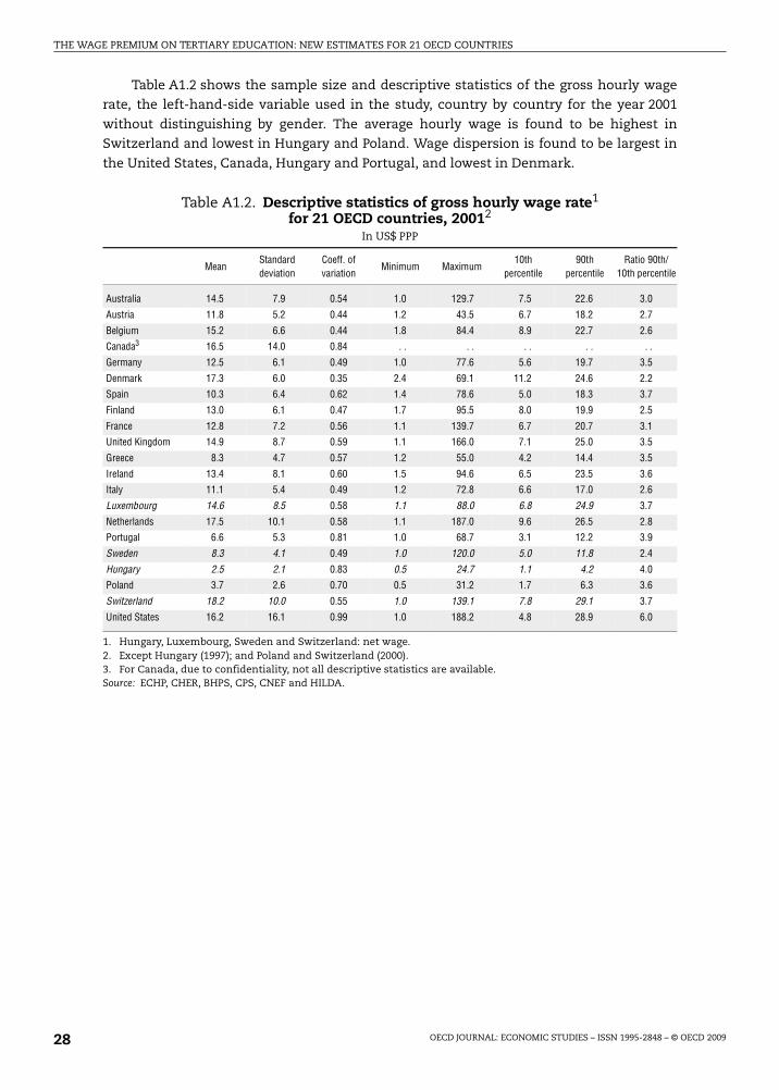
THE WAGE PREMIUM ON TERTIARY EDUCATION: NEW ESTIMATES FOR 21 OECD COUNTRIES
Table A1.2 shows the sample size and descriptive statistics of the gross hourly wagerate, the left-hand-side variable used in the study, country by country for the year 2001
without distinguishing by gender. The average hourly wage is found to be highest inSwitzerland and lowest in Hungary and Poland. Wage dispersion is found to be largest in
the United States, Canada, Hungary and Portugal, and lowest in Denmark.
Table A1.2. Descriptive statistics of gross hourly wage rate1 for 21 OECD countries, 20012
In US$ PPP
MeanStandard deviation
Coeff. of variation
Minimum Maximum10th
percentile90th
percentileRatio 90th/
10th percentile
Australia 14.5 7.9 0.54 1.0 129.7 7.5 22.6 3.0
Austria 11.8 5.2 0.44 1.2 43.5 6.7 18.2 2.7
Belgium 15.2 6.6 0.44 1.8 84.4 8.9 22.7 2.6
Canada3 16.5 14.0 0.84 . . . . . . . . . .
Germany 12.5 6.1 0.49 1.0 77.6 5.6 19.7 3.5
Denmark 17.3 6.0 0.35 2.4 69.1 11.2 24.6 2.2
Spain 10.3 6.4 0.62 1.4 78.6 5.0 18.3 3.7
Finland 13.0 6.1 0.47 1.7 95.5 8.0 19.9 2.5
France 12.8 7.2 0.56 1.1 139.7 6.7 20.7 3.1
United Kingdom 14.9 8.7 0.59 1.1 166.0 7.1 25.0 3.5
Greece 8.3 4.7 0.57 1.2 55.0 4.2 14.4 3.5
Ireland 13.4 8.1 0.60 1.5 94.6 6.5 23.5 3.6
Italy 11.1 5.4 0.49 1.2 72.8 6.6 17.0 2.6
Luxembourg 14.6 8.5 0.58 1.1 88.0 6.8 24.9 3.7
Netherlands 17.5 10.1 0.58 1.1 187.0 9.6 26.5 2.8
Portugal 6.6 5.3 0.81 1.0 68.7 3.1 12.2 3.9
Sweden 8.3 4.1 0.49 1.0 120.0 5.0 11.8 2.4
Hungary 2.5 2.1 0.83 0.5 24.7 1.1 4.2 4.0
Poland 3.7 2.6 0.70 0.5 31.2 1.7 6.3 3.6
Switzerland 18.2 10.0 0.55 1.0 139.1 7.8 29.1 3.7
United States 16.2 16.1 0.99 1.0 188.2 4.8 28.9 6.0
1. Hungary, Luxembourg, Sweden and Switzerland: net wage.2. Except Hungary (1997); and Poland and Switzerland (2000).3. For Canada, due to confidentiality, not all descriptive statistics are available.Source: ECHP, CHER, BHPS, CPS, CNEF and HILDA.
OECD JOURNAL: ECONOMIC STUDIES – ISSN 1995-2848 – © OECD 200928

TRIES
THE WAGE PREMIUM ON TERTIARY EDUCATION: NEW ESTIMATES FOR 21 OECD COUNOECD JOURNAL: ECONOMIC STUDIES – ISSN 1995-2848 – © OECD 2009 29


