
Today’s Outline - August 24, 2016
• Normalizing the wave function
• Operators: position and momentum
• The Uncertainty Principle
• Separation of variables, part I: time
• Problem 1.5
Reading Assignment: Chapter 2.3–2.4
Homework Assignment #01:Chapter 1: 1, 3, 8, 11, 15, 17due Wednesday, August 31, 2016
C. Segre (IIT) PHYS 405 - Fall 2016 August 24, 2016 1 / 20

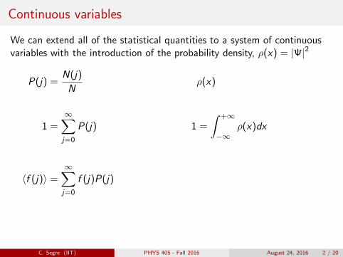
Continuous variables
We can extend all of the statistical quantities to a system of continuousvariables
with the introduction of the probability density, ρ(x) = |Ψ|2
P(j) =N(j)
Nρ(x)
1 =∞∑j=0
P(j) 1 =
∫ +∞
−∞ρ(x)dx
〈f (j)〉 =∞∑j=0
f (j)P(j) 〈f (x)〉 =
∫ +∞
−∞f (x)ρ(x)dx
σ2 ≡⟨(∆j)2
⟩=⟨j2⟩− 〈j〉2 σ2 ≡
⟨(∆x)2
⟩=⟨x2⟩− 〈x〉2
C. Segre (IIT) PHYS 405 - Fall 2016 August 24, 2016 2 / 20
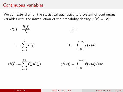
Continuous variables
We can extend all of the statistical quantities to a system of continuousvariables with the introduction of the probability density, ρ(x) = |Ψ|2
P(j) =N(j)
Nρ(x)
1 =∞∑j=0
P(j) 1 =
∫ +∞
−∞ρ(x)dx
〈f (j)〉 =∞∑j=0
f (j)P(j) 〈f (x)〉 =
∫ +∞
−∞f (x)ρ(x)dx
σ2 ≡⟨(∆j)2
⟩=⟨j2⟩− 〈j〉2 σ2 ≡
⟨(∆x)2
⟩=⟨x2⟩− 〈x〉2
C. Segre (IIT) PHYS 405 - Fall 2016 August 24, 2016 2 / 20
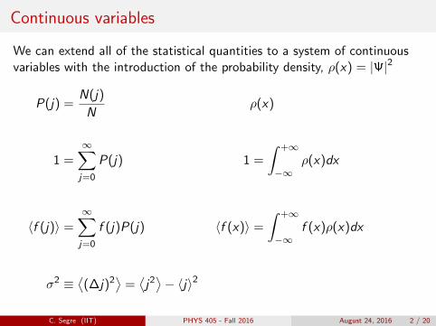
Continuous variables
We can extend all of the statistical quantities to a system of continuousvariables with the introduction of the probability density, ρ(x) = |Ψ|2
P(j) =N(j)
N
ρ(x)
1 =∞∑j=0
P(j) 1 =
∫ +∞
−∞ρ(x)dx
〈f (j)〉 =∞∑j=0
f (j)P(j) 〈f (x)〉 =
∫ +∞
−∞f (x)ρ(x)dx
σ2 ≡⟨(∆j)2
⟩=⟨j2⟩− 〈j〉2 σ2 ≡
⟨(∆x)2
⟩=⟨x2⟩− 〈x〉2
C. Segre (IIT) PHYS 405 - Fall 2016 August 24, 2016 2 / 20
Continuous variables
We can extend all of the statistical quantities to a system of continuousvariables with the introduction of the probability density, ρ(x) = |Ψ|2
P(j) =N(j)
Nρ(x)
1 =∞∑j=0
P(j) 1 =
∫ +∞
−∞ρ(x)dx
〈f (j)〉 =∞∑j=0
f (j)P(j) 〈f (x)〉 =
∫ +∞
−∞f (x)ρ(x)dx
σ2 ≡⟨(∆j)2
⟩=⟨j2⟩− 〈j〉2 σ2 ≡
⟨(∆x)2
⟩=⟨x2⟩− 〈x〉2
C. Segre (IIT) PHYS 405 - Fall 2016 August 24, 2016 2 / 20
Continuous variables
We can extend all of the statistical quantities to a system of continuousvariables with the introduction of the probability density, ρ(x) = |Ψ|2
P(j) =N(j)
Nρ(x)
1 =∞∑j=0
P(j)
1 =
∫ +∞
−∞ρ(x)dx
〈f (j)〉 =∞∑j=0
f (j)P(j) 〈f (x)〉 =
∫ +∞
−∞f (x)ρ(x)dx
σ2 ≡⟨(∆j)2
⟩=⟨j2⟩− 〈j〉2 σ2 ≡
⟨(∆x)2
⟩=⟨x2⟩− 〈x〉2
C. Segre (IIT) PHYS 405 - Fall 2016 August 24, 2016 2 / 20
Continuous variables
We can extend all of the statistical quantities to a system of continuousvariables with the introduction of the probability density, ρ(x) = |Ψ|2
P(j) =N(j)
Nρ(x)
1 =∞∑j=0
P(j) 1 =
∫ +∞
−∞ρ(x)dx
〈f (j)〉 =∞∑j=0
f (j)P(j) 〈f (x)〉 =
∫ +∞
−∞f (x)ρ(x)dx
σ2 ≡⟨(∆j)2
⟩=⟨j2⟩− 〈j〉2 σ2 ≡
⟨(∆x)2
⟩=⟨x2⟩− 〈x〉2
C. Segre (IIT) PHYS 405 - Fall 2016 August 24, 2016 2 / 20
Continuous variables
We can extend all of the statistical quantities to a system of continuousvariables with the introduction of the probability density, ρ(x) = |Ψ|2
P(j) =N(j)
Nρ(x)
1 =∞∑j=0
P(j) 1 =
∫ +∞
−∞ρ(x)dx
〈f (j)〉 =∞∑j=0
f (j)P(j)
〈f (x)〉 =
∫ +∞
−∞f (x)ρ(x)dx
σ2 ≡⟨(∆j)2
⟩=⟨j2⟩− 〈j〉2 σ2 ≡
⟨(∆x)2
⟩=⟨x2⟩− 〈x〉2
C. Segre (IIT) PHYS 405 - Fall 2016 August 24, 2016 2 / 20
Continuous variables
We can extend all of the statistical quantities to a system of continuousvariables with the introduction of the probability density, ρ(x) = |Ψ|2
P(j) =N(j)
Nρ(x)
1 =∞∑j=0
P(j) 1 =
∫ +∞
−∞ρ(x)dx
〈f (j)〉 =∞∑j=0
f (j)P(j) 〈f (x)〉 =
∫ +∞
−∞f (x)ρ(x)dx
σ2 ≡⟨(∆j)2
⟩=⟨j2⟩− 〈j〉2 σ2 ≡
⟨(∆x)2
⟩=⟨x2⟩− 〈x〉2
C. Segre (IIT) PHYS 405 - Fall 2016 August 24, 2016 2 / 20
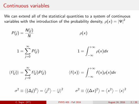
Continuous variables
We can extend all of the statistical quantities to a system of continuousvariables with the introduction of the probability density, ρ(x) = |Ψ|2
P(j) =N(j)
Nρ(x)
1 =∞∑j=0
P(j) 1 =
∫ +∞
−∞ρ(x)dx
〈f (j)〉 =∞∑j=0
f (j)P(j) 〈f (x)〉 =
∫ +∞
−∞f (x)ρ(x)dx
σ2 ≡⟨(∆j)2
⟩=⟨j2⟩− 〈j〉2
σ2 ≡⟨(∆x)2
⟩=⟨x2⟩− 〈x〉2
C. Segre (IIT) PHYS 405 - Fall 2016 August 24, 2016 2 / 20
Continuous variables
We can extend all of the statistical quantities to a system of continuousvariables with the introduction of the probability density, ρ(x) = |Ψ|2
P(j) =N(j)
Nρ(x)
1 =∞∑j=0
P(j) 1 =
∫ +∞
−∞ρ(x)dx
〈f (j)〉 =∞∑j=0
f (j)P(j) 〈f (x)〉 =
∫ +∞
−∞f (x)ρ(x)dx
σ2 ≡⟨(∆j)2
⟩=⟨j2⟩− 〈j〉2 σ2 ≡
⟨(∆x)2
⟩=⟨x2⟩− 〈x〉2
C. Segre (IIT) PHYS 405 - Fall 2016 August 24, 2016 2 / 20
Normalizing the wave function
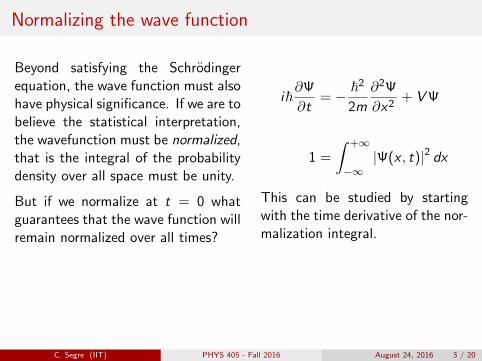
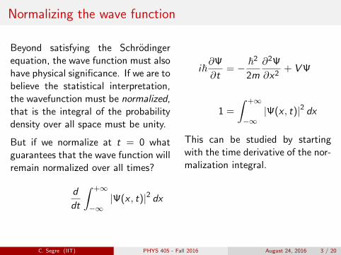
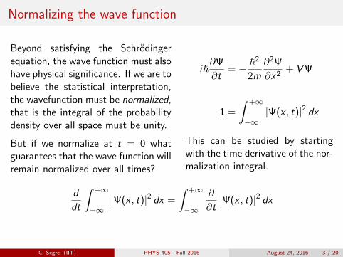
Beyond satisfying the Schrodingerequation, the wave function must alsohave physical significance.
If we are tobelieve the statistical interpretation,the wavefunction must be normalized,that is the integral of the probabilitydensity over all space must be unity.
But if we normalize at t = 0 whatguarantees that the wave function willremain normalized over all times?
i~∂Ψ
∂t= − ~2
2m
∂2Ψ
∂x2+ VΨ
1 =
∫ +∞
−∞|Ψ(x , t)|2 dx
This can be studied by startingwith the time derivative of the nor-malization integral.
d
dt
∫ +∞
−∞|Ψ(x , t)|2 dx =
∫ +∞
−∞
∂
∂t|Ψ(x , t)|2 dx
C. Segre (IIT) PHYS 405 - Fall 2016 August 24, 2016 3 / 20
Normalizing the wave function
Beyond satisfying the Schrodingerequation, the wave function must alsohave physical significance. If we are tobelieve the statistical interpretation,the wavefunction must be normalized,that is the integral of the probabilitydensity over all space must be unity.
But if we normalize at t = 0 whatguarantees that the wave function willremain normalized over all times?
i~∂Ψ
∂t= − ~2
2m
∂2Ψ
∂x2+ VΨ
1 =
∫ +∞
−∞|Ψ(x , t)|2 dx
This can be studied by startingwith the time derivative of the nor-malization integral.
d
dt
∫ +∞
−∞|Ψ(x , t)|2 dx
=
∫ +∞
−∞
∂
∂t|Ψ(x , t)|2 dx
C. Segre (IIT) PHYS 405 - Fall 2016 August 24, 2016 3 / 20
Normalizing the wave function
Beyond satisfying the Schrodingerequation, the wave function must alsohave physical significance. If we are tobelieve the statistical interpretation,the wavefunction must be normalized,that is the integral of the probabilitydensity over all space must be unity.
But if we normalize at t = 0 whatguarantees that the wave function willremain normalized over all times?
i~∂Ψ
∂t= − ~2
2m
∂2Ψ
∂x2+ VΨ
1 =
∫ +∞
−∞|Ψ(x , t)|2 dx
This can be studied by startingwith the time derivative of the nor-malization integral.
d
dt
∫ +∞
−∞|Ψ(x , t)|2 dx =
∫ +∞
−∞
∂
∂t|Ψ(x , t)|2 dx
C. Segre (IIT) PHYS 405 - Fall 2016 August 24, 2016 3 / 20

Time independence of normalization
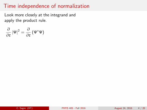
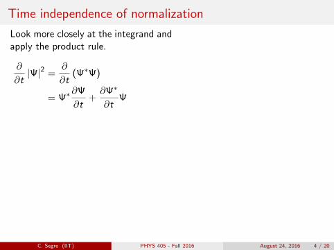
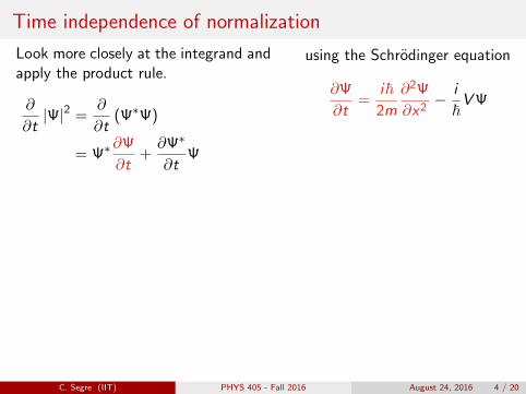
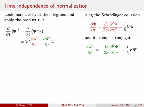
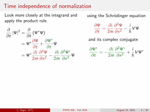
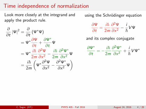
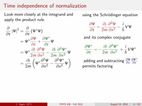
Look more closely at the integrand andapply the product rule.
∂
∂t|Ψ|2 =
∂
∂t(Ψ∗Ψ)
= Ψ∗∂Ψ
∂t+∂Ψ∗
∂tΨ
= Ψ∗i~2m
∂2Ψ
∂x2− i~
2m
∂2Ψ∗
∂x2Ψ
=i~2m
(Ψ∗
∂2Ψ
∂x2− ∂2Ψ∗
∂x2Ψ
)
using the Schrodinger equation
∂Ψ
∂t=
i~2m
∂2Ψ
∂x2− i
~VΨ
and its complex conjugate
∂Ψ∗
∂t= − i~
2m
∂2Ψ∗
∂x2+
i
~VΨ∗
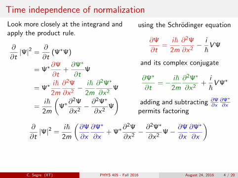
adding and subtracting ∂Ψ∂x
∂Ψ∗
∂xpermits factoring
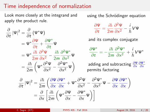
∂
∂t|Ψ|2 =
i~2m
(∂Ψ
∂x
∂Ψ∗
∂x+ Ψ∗
∂2Ψ
∂x2− ∂2Ψ∗
∂x2Ψ− ∂Ψ
∂x
∂Ψ∗
∂x
)=
∂
∂x
[i~2m
(Ψ∗
∂Ψ
∂x− ∂Ψ∗
∂xΨ
)]
C. Segre (IIT) PHYS 405 - Fall 2016 August 24, 2016 4 / 20
Time independence of normalization
Look more closely at the integrand andapply the product rule.
∂
∂t|Ψ|2 =
∂
∂t(Ψ∗Ψ)
= Ψ∗∂Ψ
∂t+∂Ψ∗
∂tΨ
= Ψ∗i~2m
∂2Ψ
∂x2− i~
2m
∂2Ψ∗
∂x2Ψ
=i~2m
(Ψ∗
∂2Ψ
∂x2− ∂2Ψ∗
∂x2Ψ
)
using the Schrodinger equation
∂Ψ
∂t=
i~2m
∂2Ψ
∂x2− i
~VΨ
and its complex conjugate
∂Ψ∗
∂t= − i~
2m
∂2Ψ∗
∂x2+
i
~VΨ∗
adding and subtracting ∂Ψ∂x
∂Ψ∗
∂xpermits factoring
∂
∂t|Ψ|2 =
i~2m
(∂Ψ
∂x
∂Ψ∗
∂x+ Ψ∗
∂2Ψ
∂x2− ∂2Ψ∗
∂x2Ψ− ∂Ψ
∂x
∂Ψ∗
∂x
)
=∂
∂x
[i~2m
(Ψ∗
∂Ψ
∂x− ∂Ψ∗
∂xΨ
)]
C. Segre (IIT) PHYS 405 - Fall 2016 August 24, 2016 4 / 20
Time independence of normalization
Look more closely at the integrand andapply the product rule.
∂
∂t|Ψ|2 =
∂
∂t(Ψ∗Ψ)
= Ψ∗∂Ψ
∂t+∂Ψ∗
∂tΨ
= Ψ∗i~2m
∂2Ψ
∂x2− i~
2m
∂2Ψ∗
∂x2Ψ
=i~2m
(Ψ∗
∂2Ψ
∂x2− ∂2Ψ∗
∂x2Ψ
)
using the Schrodinger equation
∂Ψ
∂t=
i~2m
∂2Ψ
∂x2− i
~VΨ
and its complex conjugate
∂Ψ∗
∂t= − i~
2m
∂2Ψ∗
∂x2+
i
~VΨ∗
adding and subtracting ∂Ψ∂x
∂Ψ∗
∂xpermits factoring
∂
∂t|Ψ|2 =
i~2m
(∂Ψ
∂x
∂Ψ∗
∂x+ Ψ∗
∂2Ψ
∂x2− ∂2Ψ∗
∂x2Ψ− ∂Ψ
∂x
∂Ψ∗
∂x
)=
∂
∂x
[i~2m
(Ψ∗
∂Ψ
∂x− ∂Ψ∗
∂xΨ
)]C. Segre (IIT) PHYS 405 - Fall 2016 August 24, 2016 4 / 20
Time independence of normalization
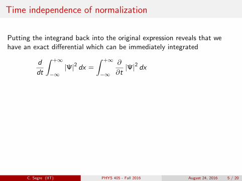
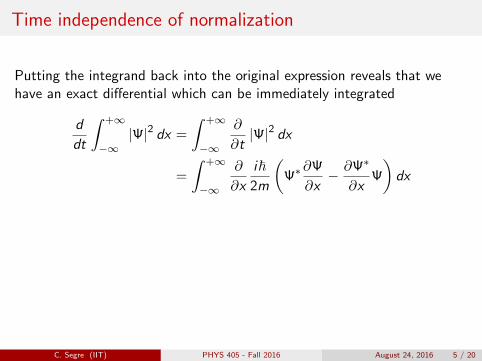
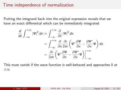
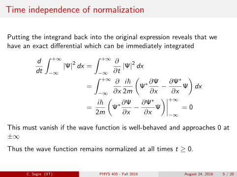
Putting the integrand back into the original expression reveals that wehave an exact differential which can be immediately integrated
d
dt
∫ +∞
−∞|Ψ|2 dx =
∫ +∞
−∞
∂
∂t|Ψ|2 dx
=
∫ +∞
−∞
∂
∂x
i~2m
(Ψ∗
∂Ψ
∂x− ∂Ψ∗
∂xΨ
)dx
=i~2m
(Ψ∗
∂Ψ
∂x− ∂Ψ∗
∂xΨ
)∣∣∣∣+∞−∞
= 0
This must vanish if the wave function is well-behaved and approaches 0 at±∞
Thus the wave function remains normalized at all times t ≥ 0.
C. Segre (IIT) PHYS 405 - Fall 2016 August 24, 2016 5 / 20
Time independence of normalization
Putting the integrand back into the original expression reveals that wehave an exact differential which can be immediately integrated
d
dt
∫ +∞
−∞|Ψ|2 dx =
∫ +∞
−∞
∂
∂t|Ψ|2 dx
=
∫ +∞
−∞
∂
∂x
i~2m
(Ψ∗
∂Ψ
∂x− ∂Ψ∗
∂xΨ
)dx
=i~2m
(Ψ∗
∂Ψ
∂x− ∂Ψ∗
∂xΨ
)∣∣∣∣+∞−∞
= 0
This must vanish if the wave function is well-behaved and approaches 0 at±∞
Thus the wave function remains normalized at all times t ≥ 0.
C. Segre (IIT) PHYS 405 - Fall 2016 August 24, 2016 5 / 20
Expectation value of position
Suppose we have many systems allprepared in the same way and all ina state described by the wave func-tion Ψ(x , t).
If we measure the position of theparticle in each of these identicalsystems, we should obtain a re-sult consistent with the expectationvalue of the position x , which iscomputed as
We can expand this and write it ina slightly different way, with the xjust to left of Ψ.
〈x〉 =
∫x |Ψ(x , t)|2 dx
=
∫Ψ∗xΨdx
In this arrangement, x is said tobe an “operator” which acts on thewave function to its right
This will eventually lead directly towhat is called the “bra-ket” no-tation commonly used in quantummechanics.
C. Segre (IIT) PHYS 405 - Fall 2016 August 24, 2016 6 / 20
Computing the velocity
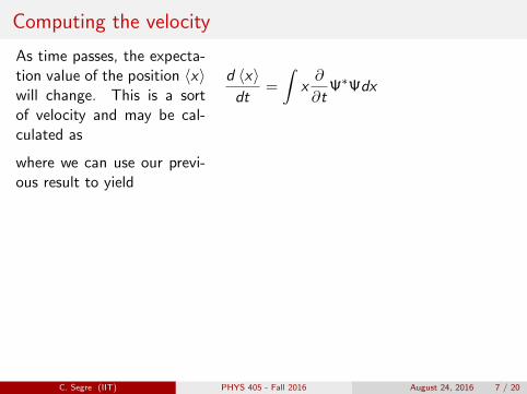
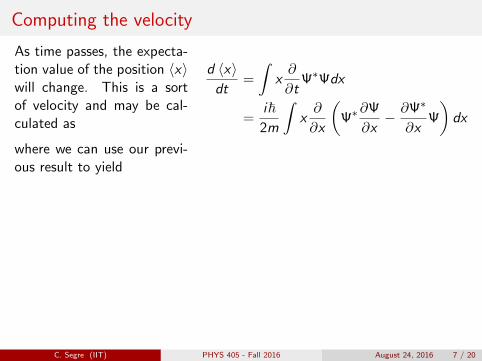
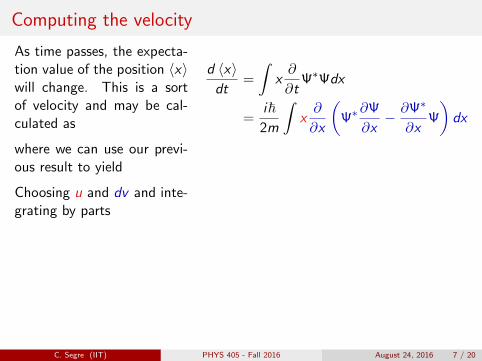
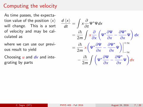
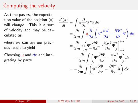
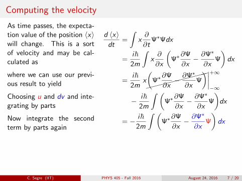
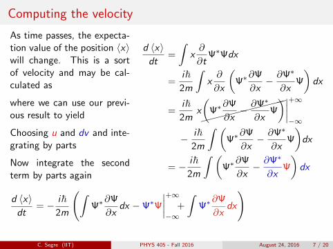
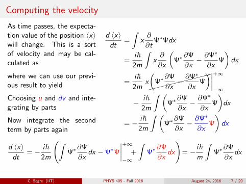
As time passes, the expecta-tion value of the position 〈x〉will change. This is a sortof velocity and may be cal-culated as
where we can use our previ-ous result to yield
Choosing u and dv and inte-grating by parts
Now integrate the secondterm by parts again
d 〈x〉dt
=
∫x∂
∂tΨ∗Ψdx
=i~2m
∫x∂
∂x
(Ψ∗
∂Ψ
∂x− ∂Ψ∗
∂xΨ
)dx
=i~2m
x����������(
Ψ∗∂Ψ
∂x− ∂Ψ∗
∂xΨ
)∣∣∣∣+∞−∞
− i~2m
∫ (Ψ∗
∂Ψ
∂x− ∂Ψ∗
∂xΨ
)dx
= − i~2m
∫ (Ψ∗
∂Ψ
∂x− ∂Ψ∗
∂xΨ
)dx
d 〈x〉dt
= − i~2m
(∫Ψ∗
∂Ψ
∂xdx −Ψ∗Ψ
∣∣∣∣+∞−∞
+
∫Ψ∗
∂Ψ
∂xdx
)= − i~
m
∫Ψ∗
∂Ψ
∂xdx
C. Segre (IIT) PHYS 405 - Fall 2016 August 24, 2016 7 / 20
Computing the velocity
As time passes, the expecta-tion value of the position 〈x〉will change. This is a sortof velocity and may be cal-culated as
where we can use our previ-ous result to yield
Choosing u and dv and inte-grating by parts
Now integrate the secondterm by parts again
d 〈x〉dt
=
∫x∂
∂tΨ∗Ψdx
=i~2m
∫x∂
∂x
(Ψ∗
∂Ψ
∂x− ∂Ψ∗
∂xΨ
)dx
=i~2m
x
(Ψ∗
∂Ψ
∂x− ∂Ψ∗
∂xΨ
)∣∣∣∣+∞−∞
− i~2m
∫ (Ψ∗
∂Ψ
∂x− ∂Ψ∗
∂xΨ
)dx
= − i~2m
∫ (Ψ∗
∂Ψ
∂x− ∂Ψ∗
∂xΨ
)dx
d 〈x〉dt
= − i~2m
(∫Ψ∗
∂Ψ
∂xdx −Ψ∗Ψ
∣∣∣∣+∞−∞
+
∫Ψ∗
∂Ψ
∂xdx
)= − i~
m
∫Ψ∗
∂Ψ
∂xdx
C. Segre (IIT) PHYS 405 - Fall 2016 August 24, 2016 7 / 20
Computing the velocity
As time passes, the expecta-tion value of the position 〈x〉will change. This is a sortof velocity and may be cal-culated as
where we can use our previ-ous result to yield
Choosing u and dv and inte-grating by parts
Now integrate the secondterm by parts again
d 〈x〉dt
=
∫x∂
∂tΨ∗Ψdx
=i~2m
∫x∂
∂x
(Ψ∗
∂Ψ
∂x− ∂Ψ∗
∂xΨ
)dx
=i~2m
x����������(
Ψ∗∂Ψ
∂x− ∂Ψ∗
∂xΨ
)∣∣∣∣+∞−∞
− i~2m
∫ (Ψ∗
∂Ψ
∂x− ∂Ψ∗
∂xΨ
)dx
= − i~2m
∫ (Ψ∗
∂Ψ
∂x− ∂Ψ∗
∂xΨ
)dx
d 〈x〉dt
= − i~2m
(∫Ψ∗
∂Ψ
∂xdx −Ψ∗Ψ
∣∣∣∣+∞−∞
+
∫Ψ∗
∂Ψ
∂xdx
)= − i~
m
∫Ψ∗
∂Ψ
∂xdx
C. Segre (IIT) PHYS 405 - Fall 2016 August 24, 2016 7 / 20
Computing the velocity
As time passes, the expecta-tion value of the position 〈x〉will change. This is a sortof velocity and may be cal-culated as
where we can use our previ-ous result to yield
Choosing u and dv and inte-grating by parts
Now integrate the secondterm by parts again
d 〈x〉dt
=
∫x∂
∂tΨ∗Ψdx
=i~2m
∫x∂
∂x
(Ψ∗
∂Ψ
∂x− ∂Ψ∗
∂xΨ
)dx
=i~2m
x����������(
Ψ∗∂Ψ
∂x− ∂Ψ∗
∂xΨ
)∣∣∣∣+∞−∞
− i~2m
∫ (Ψ∗
∂Ψ
∂x− ∂Ψ∗
∂xΨ
)dx
= − i~2m
∫ (Ψ∗
∂Ψ
∂x− ∂Ψ∗
∂xΨ
)dx
d 〈x〉dt
= − i~2m
(∫Ψ∗
∂Ψ
∂xdx −Ψ∗Ψ
∣∣∣∣+∞−∞
+
∫Ψ∗
∂Ψ
∂xdx
)
= − i~m
∫Ψ∗
∂Ψ
∂xdx
C. Segre (IIT) PHYS 405 - Fall 2016 August 24, 2016 7 / 20
Computing the velocity
As time passes, the expecta-tion value of the position 〈x〉will change. This is a sortof velocity and may be cal-culated as
where we can use our previ-ous result to yield
Choosing u and dv and inte-grating by parts
Now integrate the secondterm by parts again
d 〈x〉dt
=
∫x∂
∂tΨ∗Ψdx
=i~2m
∫x∂
∂x
(Ψ∗
∂Ψ
∂x− ∂Ψ∗
∂xΨ
)dx
=i~2m
x����������(
Ψ∗∂Ψ
∂x− ∂Ψ∗
∂xΨ
)∣∣∣∣+∞−∞
− i~2m
∫ (Ψ∗
∂Ψ
∂x− ∂Ψ∗
∂xΨ
)dx
= − i~2m
∫ (Ψ∗
∂Ψ
∂x− ∂Ψ∗
∂xΨ
)dx
d 〈x〉dt
= − i~2m
(∫Ψ∗
∂Ψ
∂xdx −Ψ∗Ψ
∣∣∣∣+∞−∞
+
∫Ψ∗
∂Ψ
∂xdx
)= − i~
m
∫Ψ∗
∂Ψ
∂xdx
C. Segre (IIT) PHYS 405 - Fall 2016 August 24, 2016 7 / 20
Momentum operator
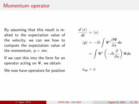
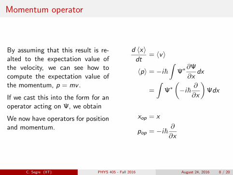
By assuming that this result is re-alted to the expectation value ofthe velocity, we can see how tocompute the expectation value ofthe momentum, p = mv .
If we cast this into the form for anoperator acting on Ψ, we obtain
We now have operators for positionand momentum.
d 〈x〉dt
= 〈v〉
〈p〉 = −i~∫
Ψ∗∂Ψ
∂xdx
=
∫Ψ∗(−i~ ∂
∂x
)Ψdx
xop = x
pop = −i~ ∂∂x
C. Segre (IIT) PHYS 405 - Fall 2016 August 24, 2016 8 / 20
Momentum operator
By assuming that this result is re-alted to the expectation value ofthe velocity, we can see how tocompute the expectation value ofthe momentum, p = mv .
If we cast this into the form for anoperator acting on Ψ, we obtain
We now have operators for positionand momentum.
d 〈x〉dt
= 〈v〉
〈p〉 = −i~∫
Ψ∗∂Ψ
∂xdx
=
∫Ψ∗(−i~ ∂
∂x
)Ψdx
xop = x
pop = −i~ ∂∂x
C. Segre (IIT) PHYS 405 - Fall 2016 August 24, 2016 8 / 20

Momentum operator
By assuming that this result is re-alted to the expectation value ofthe velocity, we can see how tocompute the expectation value ofthe momentum, p = mv .
If we cast this into the form for anoperator acting on Ψ, we obtain
We now have operators for position
and momentum.
d 〈x〉dt
= 〈v〉
〈p〉 = −i~∫
Ψ∗∂Ψ
∂xdx
=
∫Ψ∗(−i~ ∂
∂x
)Ψdx
xop = x
pop = −i~ ∂∂x
C. Segre (IIT) PHYS 405 - Fall 2016 August 24, 2016 8 / 20
Momentum operator
By assuming that this result is re-alted to the expectation value ofthe velocity, we can see how tocompute the expectation value ofthe momentum, p = mv .
If we cast this into the form for anoperator acting on Ψ, we obtain
We now have operators for positionand momentum.
d 〈x〉dt
= 〈v〉
〈p〉 = −i~∫
Ψ∗∂Ψ
∂xdx
=
∫Ψ∗(−i~ ∂
∂x
)Ψdx
xop = x
pop = −i~ ∂∂x
C. Segre (IIT) PHYS 405 - Fall 2016 August 24, 2016 8 / 20
Operators
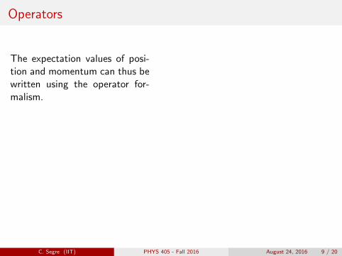
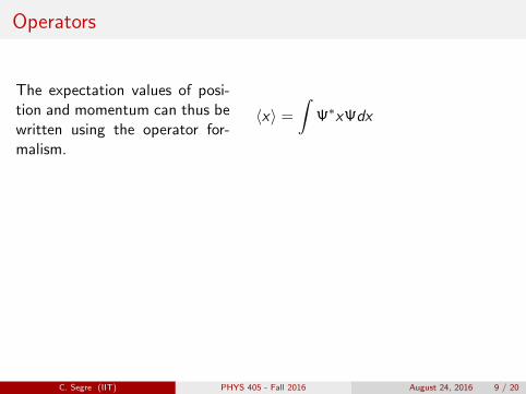
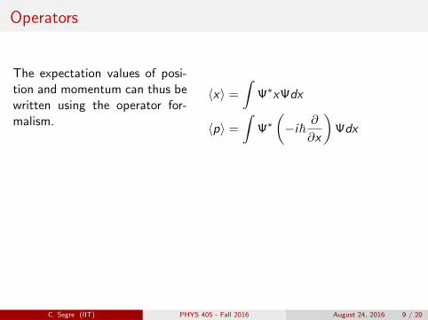
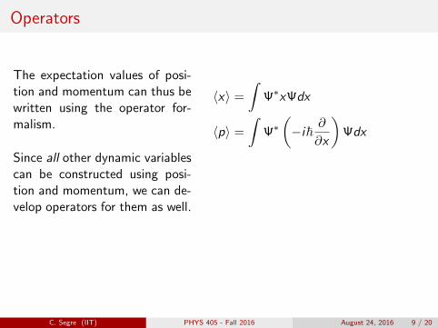
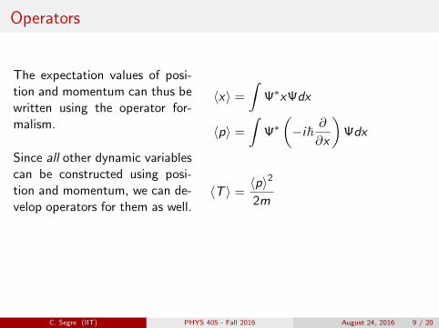
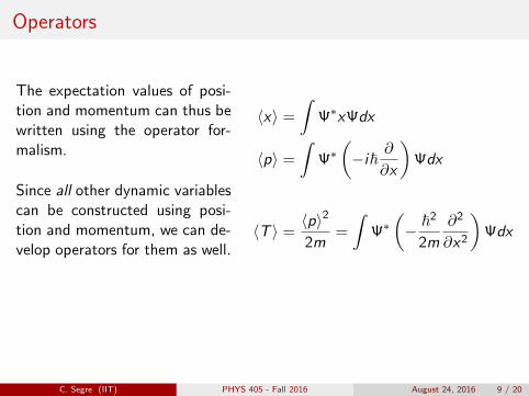
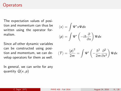
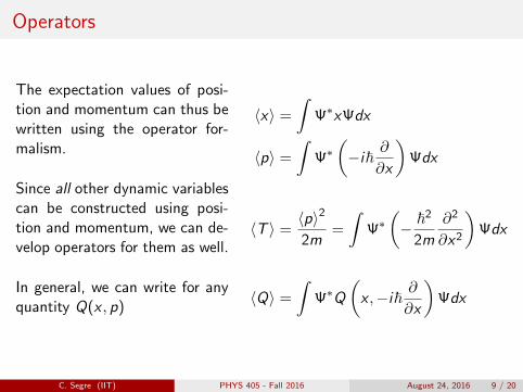
The expectation values of posi-tion and momentum can thus bewritten using the operator for-malism.
Since all other dynamic variablescan be constructed using posi-tion and momentum, we can de-velop operators for them as well.
In general, we can write for anyquantity Q(x , p)
〈x〉 =
∫Ψ∗xΨdx
〈p〉 =
∫Ψ∗(−i~ ∂
∂x
)Ψdx
〈T 〉 =〈p〉2
2m=
∫Ψ∗(− ~2
2m
∂2
∂x2
)Ψdx
〈Q〉 =
∫Ψ∗Q
(x ,−i~ ∂
∂x
)Ψdx
C. Segre (IIT) PHYS 405 - Fall 2016 August 24, 2016 9 / 20
Operators
The expectation values of posi-tion and momentum can thus bewritten using the operator for-malism.
Since all other dynamic variablescan be constructed using posi-tion and momentum, we can de-velop operators for them as well.
In general, we can write for anyquantity Q(x , p)
〈x〉 =
∫Ψ∗xΨdx
〈p〉 =
∫Ψ∗(−i~ ∂
∂x
)Ψdx
〈T 〉 =〈p〉2
2m
=
∫Ψ∗(− ~2
2m
∂2
∂x2
)Ψdx
〈Q〉 =
∫Ψ∗Q
(x ,−i~ ∂
∂x
)Ψdx
C. Segre (IIT) PHYS 405 - Fall 2016 August 24, 2016 9 / 20
Operators
The expectation values of posi-tion and momentum can thus bewritten using the operator for-malism.
Since all other dynamic variablescan be constructed using posi-tion and momentum, we can de-velop operators for them as well.
In general, we can write for anyquantity Q(x , p)
〈x〉 =
∫Ψ∗xΨdx
〈p〉 =
∫Ψ∗(−i~ ∂
∂x
)Ψdx
〈T 〉 =〈p〉2
2m=
∫Ψ∗(− ~2
2m
∂2
∂x2
)Ψdx
〈Q〉 =
∫Ψ∗Q
(x ,−i~ ∂
∂x
)Ψdx
C. Segre (IIT) PHYS 405 - Fall 2016 August 24, 2016 9 / 20
Operators
The expectation values of posi-tion and momentum can thus bewritten using the operator for-malism.
Since all other dynamic variablescan be constructed using posi-tion and momentum, we can de-velop operators for them as well.
In general, we can write for anyquantity Q(x , p)
〈x〉 =
∫Ψ∗xΨdx
〈p〉 =
∫Ψ∗(−i~ ∂
∂x
)Ψdx
〈T 〉 =〈p〉2
2m=
∫Ψ∗(− ~2
2m
∂2
∂x2
)Ψdx
〈Q〉 =
∫Ψ∗Q
(x ,−i~ ∂
∂x
)Ψdx
C. Segre (IIT) PHYS 405 - Fall 2016 August 24, 2016 9 / 20
Ehrenfest Theorem
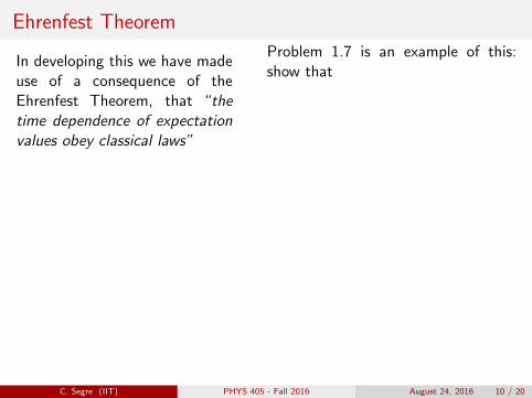
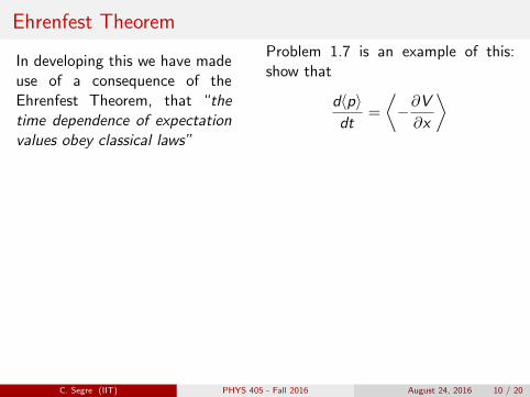
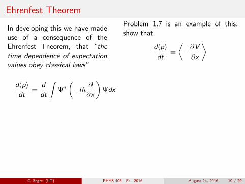
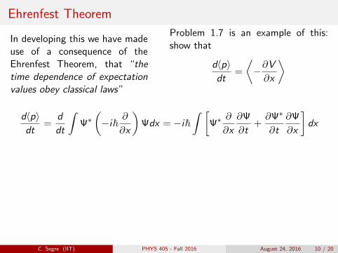
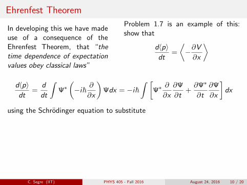
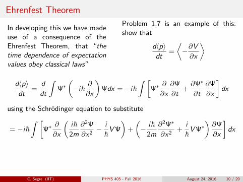
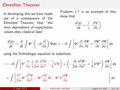
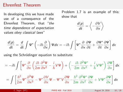
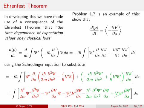
In developing this we have madeuse of a consequence of theEhrenfest Theorem, that “thetime dependence of expectationvalues obey classical laws”
Problem 1.7 is an example of this:show that
d〈p〉dt
=
⟨−∂V∂x
⟩
d〈p〉dt
=d
dt
∫Ψ∗(−i~ ∂
∂x
)Ψdx = −i~
∫ [Ψ∗
∂
∂x
∂Ψ
∂t+∂Ψ∗
∂t
∂Ψ
∂x
]dx
using the Schrodinger equation to substitute
= −i~∫ [
Ψ∗∂
∂x
(i~2m
∂2Ψ
∂x2− i
~VΨ
)+
(− i~
2m
∂2Ψ∗
∂x2+
i
~VΨ∗
)∂Ψ
∂x
]dx
=
∫ [~2
2mΨ∗
∂3Ψ
∂x3−Ψ∗
∂V
∂xΨ−
�����
Ψ∗V∂Ψ
∂x
− ~2
2m
∂2Ψ∗
∂x2
∂Ψ
∂x+���
��VΨ∗
∂Ψ
∂x
]dx
C. Segre (IIT) PHYS 405 - Fall 2016 August 24, 2016 10 / 20
Ehrenfest Theorem
In developing this we have madeuse of a consequence of theEhrenfest Theorem, that “thetime dependence of expectationvalues obey classical laws”
Problem 1.7 is an example of this:show that
d〈p〉dt
=
⟨−∂V∂x
⟩
d〈p〉dt
=d
dt
∫Ψ∗(−i~ ∂
∂x
)Ψdx
= −i~∫ [
Ψ∗∂
∂x
∂Ψ
∂t+∂Ψ∗
∂t
∂Ψ
∂x
]dx
using the Schrodinger equation to substitute
= −i~∫ [
Ψ∗∂
∂x
(i~2m
∂2Ψ
∂x2− i
~VΨ
)+
(− i~
2m
∂2Ψ∗
∂x2+
i
~VΨ∗
)∂Ψ
∂x
]dx
=
∫ [~2
2mΨ∗
∂3Ψ
∂x3−Ψ∗
∂V
∂xΨ−
�����
Ψ∗V∂Ψ
∂x
− ~2
2m
∂2Ψ∗
∂x2
∂Ψ
∂x+���
��VΨ∗
∂Ψ
∂x
]dx
C. Segre (IIT) PHYS 405 - Fall 2016 August 24, 2016 10 / 20
Ehrenfest Theorem
In developing this we have madeuse of a consequence of theEhrenfest Theorem, that “thetime dependence of expectationvalues obey classical laws”
Problem 1.7 is an example of this:show that
d〈p〉dt
=
⟨−∂V∂x
⟩
d〈p〉dt
=d
dt
∫Ψ∗(−i~ ∂
∂x
)Ψdx = −i~
∫ [Ψ∗
∂
∂x
∂Ψ
∂t+∂Ψ∗
∂t
∂Ψ
∂x
]dx
using the Schrodinger equation to substitute
= −i~∫ [
Ψ∗∂
∂x
(i~2m
∂2Ψ
∂x2− i
~VΨ
)+
(− i~
2m
∂2Ψ∗
∂x2+
i
~VΨ∗
)∂Ψ
∂x
]dx
=
∫ [~2
2mΨ∗
∂3Ψ
∂x3−Ψ∗
∂V
∂xΨ−
�����
Ψ∗V∂Ψ
∂x
− ~2
2m
∂2Ψ∗
∂x2
∂Ψ
∂x+���
��VΨ∗
∂Ψ
∂x
]dx
C. Segre (IIT) PHYS 405 - Fall 2016 August 24, 2016 10 / 20
Ehrenfest Theorem
In developing this we have madeuse of a consequence of theEhrenfest Theorem, that “thetime dependence of expectationvalues obey classical laws”
Problem 1.7 is an example of this:show that
d〈p〉dt
=
⟨−∂V∂x
⟩
d〈p〉dt
=d
dt
∫Ψ∗(−i~ ∂
∂x
)Ψdx = −i~
∫ [Ψ∗
∂
∂x
∂Ψ
∂t+∂Ψ∗
∂t
∂Ψ
∂x
]dx
using the Schrodinger equation to substitute
= −i~∫ [
Ψ∗∂
∂x
(i~2m
∂2Ψ
∂x2− i
~VΨ
)+
(− i~
2m
∂2Ψ∗
∂x2+
i
~VΨ∗
)∂Ψ
∂x
]dx
=
∫ [~2
2mΨ∗
∂3Ψ
∂x3−Ψ∗
∂V
∂xΨ−Ψ∗V
∂Ψ
∂x
− ~2
2m
∂2Ψ∗
∂x2
∂Ψ
∂x+���
��VΨ∗
∂Ψ
∂x
]dx
C. Segre (IIT) PHYS 405 - Fall 2016 August 24, 2016 10 / 20
Ehrenfest Theorem
In developing this we have madeuse of a consequence of theEhrenfest Theorem, that “thetime dependence of expectationvalues obey classical laws”
Problem 1.7 is an example of this:show that
d〈p〉dt
=
⟨−∂V∂x
⟩
d〈p〉dt
=d
dt
∫Ψ∗(−i~ ∂
∂x
)Ψdx = −i~
∫ [Ψ∗
∂
∂x
∂Ψ
∂t+∂Ψ∗
∂t
∂Ψ
∂x
]dx
using the Schrodinger equation to substitute
= −i~∫ [
Ψ∗∂
∂x
(i~2m
∂2Ψ
∂x2− i
~VΨ
)+
(− i~
2m
∂2Ψ∗
∂x2+
i
~VΨ∗
)∂Ψ
∂x
]dx
=
∫ [~2
2mΨ∗
∂3Ψ
∂x3−Ψ∗
∂V
∂xΨ−Ψ∗V
∂Ψ
∂x− ~2
2m
∂2Ψ∗
∂x2
∂Ψ
∂x+ VΨ∗
∂Ψ
∂x
]dx
C. Segre (IIT) PHYS 405 - Fall 2016 August 24, 2016 10 / 20
Ehrenfest Theorem
In developing this we have madeuse of a consequence of theEhrenfest Theorem, that “thetime dependence of expectationvalues obey classical laws”
Problem 1.7 is an example of this:show that
d〈p〉dt
=
⟨−∂V∂x
⟩
d〈p〉dt
=d
dt
∫Ψ∗(−i~ ∂
∂x
)Ψdx = −i~
∫ [Ψ∗
∂
∂x
∂Ψ
∂t+∂Ψ∗
∂t
∂Ψ
∂x
]dx
using the Schrodinger equation to substitute
= −i~∫ [
Ψ∗∂
∂x
(i~2m
∂2Ψ
∂x2− i
~VΨ
)+
(− i~
2m
∂2Ψ∗
∂x2+
i
~VΨ∗
)∂Ψ
∂x
]dx
=
∫ [~2
2mΨ∗
∂3Ψ
∂x3−Ψ∗
∂V
∂xΨ−
�����
Ψ∗V∂Ψ
∂x− ~2
2m
∂2Ψ∗
∂x2
∂Ψ
∂x+���
��VΨ∗
∂Ψ
∂x
]dx
C. Segre (IIT) PHYS 405 - Fall 2016 August 24, 2016 10 / 20
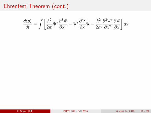
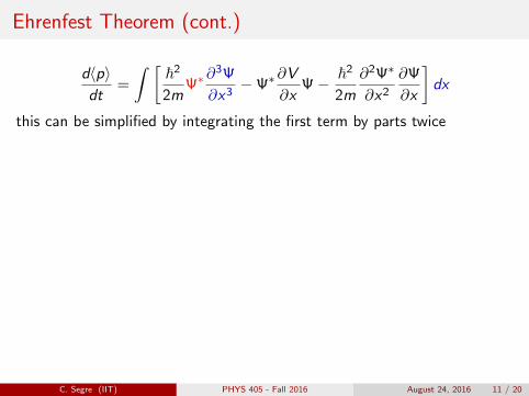
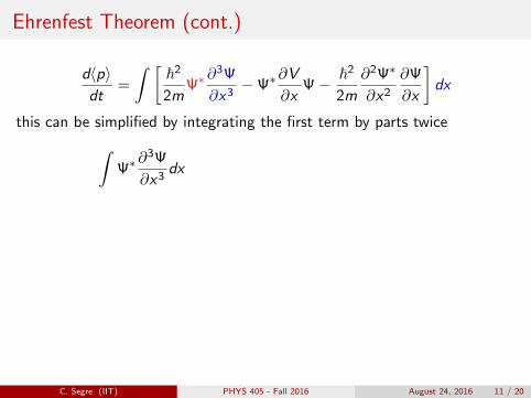
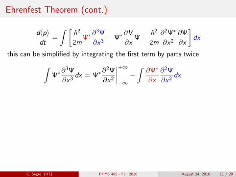
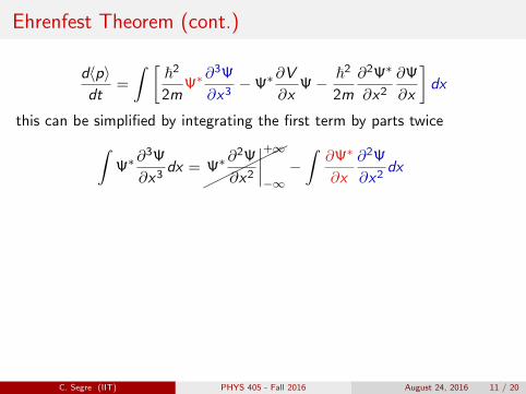
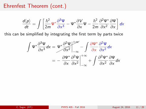
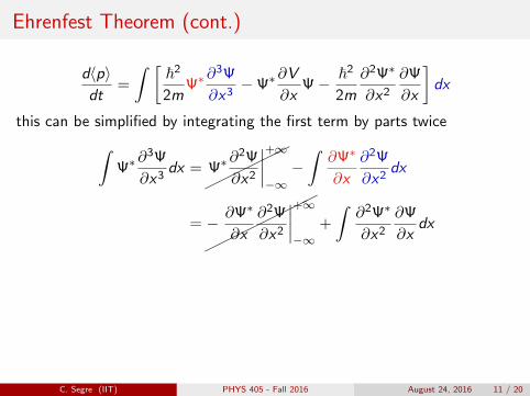
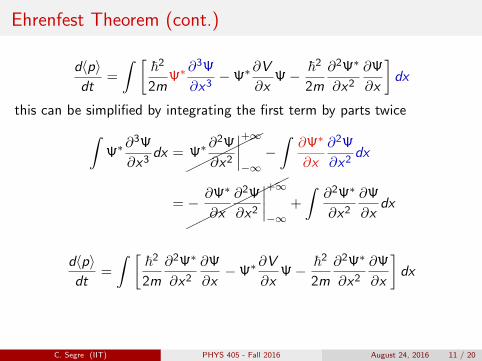
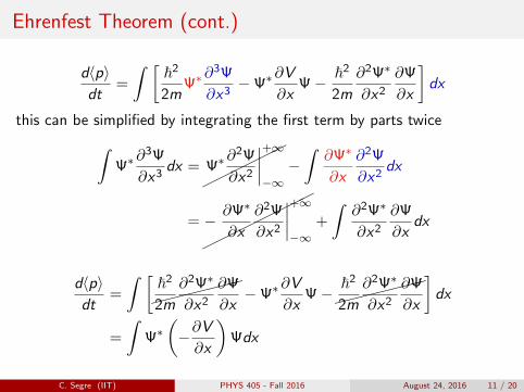
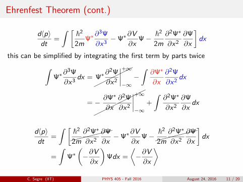
Ehrenfest Theorem (cont.)
d〈p〉dt
=
∫ [~2
2mΨ∗
∂3Ψ
∂x3−Ψ∗
∂V
∂xΨ− ~2
2m
∂2Ψ∗
∂x2
∂Ψ
∂x
]dx
this can be simplified by integrating the first term by parts twice∫Ψ∗
∂3Ψ
∂x3dx =
������
Ψ∗∂2Ψ
∂x2
∣∣∣∣+∞−∞−∫∂Ψ∗
∂x
∂2Ψ
∂x2dx
=
�����
���
− ∂Ψ∗
∂x
∂2Ψ
∂x2
∣∣∣∣+∞−∞
+
∫∂2Ψ∗
∂x2
∂Ψ
∂xdx
d〈p〉dt
=
∫ [�������~2
2m
∂2Ψ∗
∂x2
∂Ψ
∂x−Ψ∗
∂V
∂xΨ−�������~2
2m
∂2Ψ∗
∂x2
∂Ψ
∂x
]dx
=
∫Ψ∗(−∂V∂x
)Ψdx =
⟨−∂V∂x
⟩
C. Segre (IIT) PHYS 405 - Fall 2016 August 24, 2016 11 / 20
Ehrenfest Theorem (cont.)
d〈p〉dt
=
∫ [~2
2mΨ∗
∂3Ψ
∂x3−Ψ∗
∂V
∂xΨ− ~2
2m
∂2Ψ∗
∂x2
∂Ψ
∂x
]dx
this can be simplified by integrating the first term by parts twice
∫Ψ∗
∂3Ψ
∂x3dx =
������
Ψ∗∂2Ψ
∂x2
∣∣∣∣+∞−∞−∫∂Ψ∗
∂x
∂2Ψ
∂x2dx
=
�����
���
− ∂Ψ∗
∂x
∂2Ψ
∂x2
∣∣∣∣+∞−∞
+
∫∂2Ψ∗
∂x2
∂Ψ
∂xdx
d〈p〉dt
=
∫ [�������~2
2m
∂2Ψ∗
∂x2
∂Ψ
∂x−Ψ∗
∂V
∂xΨ−�������~2
2m
∂2Ψ∗
∂x2
∂Ψ
∂x
]dx
=
∫Ψ∗(−∂V∂x
)Ψdx =
⟨−∂V∂x
⟩
C. Segre (IIT) PHYS 405 - Fall 2016 August 24, 2016 11 / 20
Ehrenfest Theorem (cont.)
d〈p〉dt
=
∫ [~2
2mΨ∗
∂3Ψ
∂x3−Ψ∗
∂V
∂xΨ− ~2
2m
∂2Ψ∗
∂x2
∂Ψ
∂x
]dx
this can be simplified by integrating the first term by parts twice∫Ψ∗
∂3Ψ
∂x3dx
=���
���
Ψ∗∂2Ψ
∂x2
∣∣∣∣+∞−∞−∫∂Ψ∗
∂x
∂2Ψ
∂x2dx
=
�����
���
− ∂Ψ∗
∂x
∂2Ψ
∂x2
∣∣∣∣+∞−∞
+
∫∂2Ψ∗
∂x2
∂Ψ
∂xdx
d〈p〉dt
=
∫ [�������~2
2m
∂2Ψ∗
∂x2
∂Ψ
∂x−Ψ∗
∂V
∂xΨ−�������~2
2m
∂2Ψ∗
∂x2
∂Ψ
∂x
]dx
=
∫Ψ∗(−∂V∂x
)Ψdx =
⟨−∂V∂x
⟩
C. Segre (IIT) PHYS 405 - Fall 2016 August 24, 2016 11 / 20
Ehrenfest Theorem (cont.)
d〈p〉dt
=
∫ [~2
2mΨ∗
∂3Ψ
∂x3−Ψ∗
∂V
∂xΨ− ~2
2m
∂2Ψ∗
∂x2
∂Ψ
∂x
]dx
this can be simplified by integrating the first term by parts twice∫Ψ∗
∂3Ψ
∂x3dx = Ψ∗
∂2Ψ
∂x2
∣∣∣∣+∞−∞−∫∂Ψ∗
∂x
∂2Ψ
∂x2dx
=
����
����
− ∂Ψ∗
∂x
∂2Ψ
∂x2
∣∣∣∣+∞−∞
+
∫∂2Ψ∗
∂x2
∂Ψ
∂xdx
d〈p〉dt
=
∫ [�������~2
2m
∂2Ψ∗
∂x2
∂Ψ
∂x−Ψ∗
∂V
∂xΨ−�������~2
2m
∂2Ψ∗
∂x2
∂Ψ
∂x
]dx
=
∫Ψ∗(−∂V∂x
)Ψdx =
⟨−∂V∂x
⟩
C. Segre (IIT) PHYS 405 - Fall 2016 August 24, 2016 11 / 20
Ehrenfest Theorem (cont.)
d〈p〉dt
=
∫ [~2
2mΨ∗
∂3Ψ
∂x3−Ψ∗
∂V
∂xΨ− ~2
2m
∂2Ψ∗
∂x2
∂Ψ
∂x
]dx
this can be simplified by integrating the first term by parts twice∫Ψ∗
∂3Ψ
∂x3dx =
������
Ψ∗∂2Ψ
∂x2
∣∣∣∣+∞−∞−∫∂Ψ∗
∂x
∂2Ψ
∂x2dx
=
�����
���
− ∂Ψ∗
∂x
∂2Ψ
∂x2
∣∣∣∣+∞−∞
+
∫∂2Ψ∗
∂x2
∂Ψ
∂xdx
d〈p〉dt
=
∫ [�������~2
2m
∂2Ψ∗
∂x2
∂Ψ
∂x−Ψ∗
∂V
∂xΨ−�������~2
2m
∂2Ψ∗
∂x2
∂Ψ
∂x
]dx
=
∫Ψ∗(−∂V∂x
)Ψdx =
⟨−∂V∂x
⟩
C. Segre (IIT) PHYS 405 - Fall 2016 August 24, 2016 11 / 20
Ehrenfest Theorem (cont.)
d〈p〉dt
=
∫ [~2
2mΨ∗
∂3Ψ
∂x3−Ψ∗
∂V
∂xΨ− ~2
2m
∂2Ψ∗
∂x2
∂Ψ
∂x
]dx
this can be simplified by integrating the first term by parts twice∫Ψ∗
∂3Ψ
∂x3dx =
������
Ψ∗∂2Ψ
∂x2
∣∣∣∣+∞−∞−∫∂Ψ∗
∂x
∂2Ψ
∂x2dx
= − ∂Ψ∗
∂x
∂2Ψ
∂x2
∣∣∣∣+∞−∞
+
∫∂2Ψ∗
∂x2
∂Ψ
∂xdx
d〈p〉dt
=
∫ [�������~2
2m
∂2Ψ∗
∂x2
∂Ψ
∂x−Ψ∗
∂V
∂xΨ−�������~2
2m
∂2Ψ∗
∂x2
∂Ψ
∂x
]dx
=
∫Ψ∗(−∂V∂x
)Ψdx =
⟨−∂V∂x
⟩
C. Segre (IIT) PHYS 405 - Fall 2016 August 24, 2016 11 / 20
Ehrenfest Theorem (cont.)
d〈p〉dt
=
∫ [~2
2mΨ∗
∂3Ψ
∂x3−Ψ∗
∂V
∂xΨ− ~2
2m
∂2Ψ∗
∂x2
∂Ψ
∂x
]dx
this can be simplified by integrating the first term by parts twice∫Ψ∗
∂3Ψ
∂x3dx =
������
Ψ∗∂2Ψ
∂x2
∣∣∣∣+∞−∞−∫∂Ψ∗
∂x
∂2Ψ
∂x2dx
=
�����
���
− ∂Ψ∗
∂x
∂2Ψ
∂x2
∣∣∣∣+∞−∞
+
∫∂2Ψ∗
∂x2
∂Ψ
∂xdx
d〈p〉dt
=
∫ [�������~2
2m
∂2Ψ∗
∂x2
∂Ψ
∂x−Ψ∗
∂V
∂xΨ−�������~2
2m
∂2Ψ∗
∂x2
∂Ψ
∂x
]dx
=
∫Ψ∗(−∂V∂x
)Ψdx =
⟨−∂V∂x
⟩
C. Segre (IIT) PHYS 405 - Fall 2016 August 24, 2016 11 / 20
Ehrenfest Theorem (cont.)
d〈p〉dt
=
∫ [~2
2mΨ∗
∂3Ψ
∂x3−Ψ∗
∂V
∂xΨ− ~2
2m
∂2Ψ∗
∂x2
∂Ψ
∂x
]dx
this can be simplified by integrating the first term by parts twice∫Ψ∗
∂3Ψ
∂x3dx =
������
Ψ∗∂2Ψ
∂x2
∣∣∣∣+∞−∞−∫∂Ψ∗
∂x
∂2Ψ
∂x2dx
=
����
����
− ∂Ψ∗
∂x
∂2Ψ
∂x2
∣∣∣∣+∞−∞
+
∫∂2Ψ∗
∂x2
∂Ψ
∂xdx
d〈p〉dt
=
∫ [~2
2m
∂2Ψ∗
∂x2
∂Ψ
∂x−Ψ∗
∂V
∂xΨ− ~2
2m
∂2Ψ∗
∂x2
∂Ψ
∂x
]dx
=
∫Ψ∗(−∂V∂x
)Ψdx =
⟨−∂V∂x
⟩
C. Segre (IIT) PHYS 405 - Fall 2016 August 24, 2016 11 / 20
Ehrenfest Theorem (cont.)
d〈p〉dt
=
∫ [~2
2mΨ∗
∂3Ψ
∂x3−Ψ∗
∂V
∂xΨ− ~2
2m
∂2Ψ∗
∂x2
∂Ψ
∂x
]dx
this can be simplified by integrating the first term by parts twice∫Ψ∗
∂3Ψ
∂x3dx =
������
Ψ∗∂2Ψ
∂x2
∣∣∣∣+∞−∞−∫∂Ψ∗
∂x
∂2Ψ
∂x2dx
=
�����
���
− ∂Ψ∗
∂x
∂2Ψ
∂x2
∣∣∣∣+∞−∞
+
∫∂2Ψ∗
∂x2
∂Ψ
∂xdx
d〈p〉dt
=
∫ [�������~2
2m
∂2Ψ∗
∂x2
∂Ψ
∂x−Ψ∗
∂V
∂xΨ−�������~2
2m
∂2Ψ∗
∂x2
∂Ψ
∂x
]dx
=
∫Ψ∗(−∂V∂x
)Ψdx
=
⟨−∂V∂x
⟩
C. Segre (IIT) PHYS 405 - Fall 2016 August 24, 2016 11 / 20
Ehrenfest Theorem (cont.)
d〈p〉dt
=
∫ [~2
2mΨ∗
∂3Ψ
∂x3−Ψ∗
∂V
∂xΨ− ~2
2m
∂2Ψ∗
∂x2
∂Ψ
∂x
]dx
this can be simplified by integrating the first term by parts twice∫Ψ∗
∂3Ψ
∂x3dx =
������
Ψ∗∂2Ψ
∂x2
∣∣∣∣+∞−∞−∫∂Ψ∗
∂x
∂2Ψ
∂x2dx
=
�����
���
− ∂Ψ∗
∂x
∂2Ψ
∂x2
∣∣∣∣+∞−∞
+
∫∂2Ψ∗
∂x2
∂Ψ
∂xdx
d〈p〉dt
=
∫ [�������~2
2m
∂2Ψ∗
∂x2
∂Ψ
∂x−Ψ∗
∂V
∂xΨ−�������~2
2m
∂2Ψ∗
∂x2
∂Ψ
∂x
]dx
=
∫Ψ∗(−∂V∂x
)Ψdx =
⟨−∂V∂x
⟩C. Segre (IIT) PHYS 405 - Fall 2016 August 24, 2016 11 / 20
Uncertainty Principle
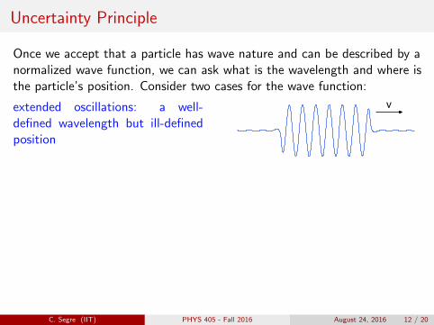
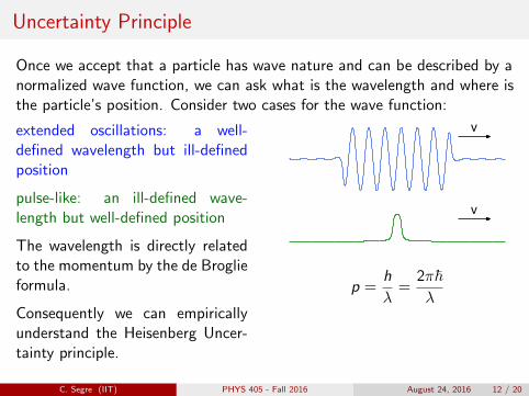
Once we accept that a particle has wave nature and can be described by anormalized wave function, we can ask what is the wavelength and where isthe particle’s position.
Consider two cases for the wave function:
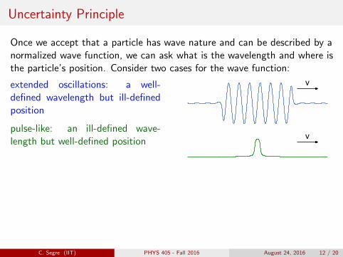
extended oscillations: a well-defined wavelength but ill-definedposition
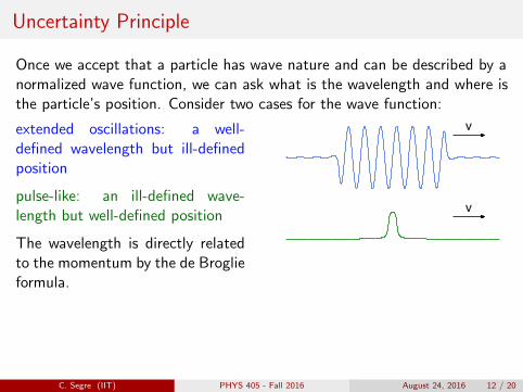
pulse-like: an ill-defined wave-length but well-defined position
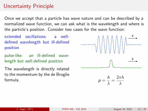
The wavelength is directly relatedto the momentum by the de Broglieformula.
Consequently we can empiricallyunderstand the Heisenberg Uncer-tainty principle.
v
v
p =h
λ=
2π~λ
σxσp ≥~2
C. Segre (IIT) PHYS 405 - Fall 2016 August 24, 2016 12 / 20
Uncertainty Principle
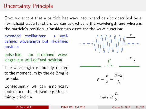
Once we accept that a particle has wave nature and can be described by anormalized wave function, we can ask what is the wavelength and where isthe particle’s position. Consider two cases for the wave function:
extended oscillations: a well-defined wavelength but ill-definedposition
pulse-like: an ill-defined wave-length but well-defined position
The wavelength is directly relatedto the momentum by the de Broglieformula.
Consequently we can empiricallyunderstand the Heisenberg Uncer-tainty principle.
v
v
p =h
λ=
2π~λ
σxσp ≥~2
C. Segre (IIT) PHYS 405 - Fall 2016 August 24, 2016 12 / 20
Uncertainty Principle
Once we accept that a particle has wave nature and can be described by anormalized wave function, we can ask what is the wavelength and where isthe particle’s position. Consider two cases for the wave function:
extended oscillations: a well-defined wavelength but ill-definedposition
pulse-like: an ill-defined wave-length but well-defined position
The wavelength is directly relatedto the momentum by the de Broglieformula.
Consequently we can empiricallyunderstand the Heisenberg Uncer-tainty principle.
v
v
p =h
λ=
2π~λ
σxσp ≥~2
C. Segre (IIT) PHYS 405 - Fall 2016 August 24, 2016 12 / 20
Time independent Schrodinger equation
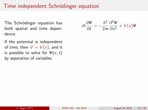
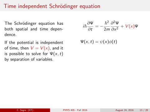
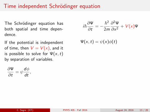
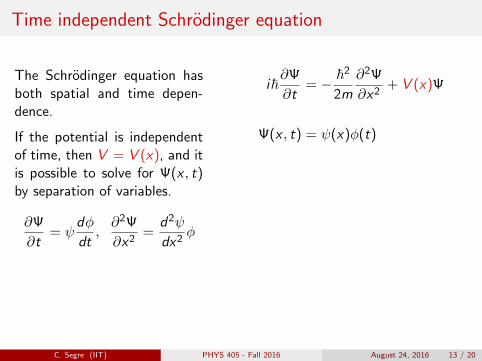
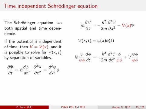
The Schrodinger equation hasboth spatial and time depen-dence.
If the potential is independentof time, then V = V (x), and itis possible to solve for Ψ(x , t)by separation of variables.
∂Ψ
∂t= ψ
dφ
dt,∂2Ψ
∂x2=
d2ψ
dx2φ
This can be solved only if eachside of the separable equation isa constant, E .
i~∂Ψ
∂t= − ~2
2m
∂2Ψ
∂x2+ V (x)Ψ
Ψ(x , t) = ψ(x)φ(t)
i~ψ
ψφ
dφ
dt= − ~2
2m
d2ψ
dx2
φ
ψφ+ V
ψφ
ψφ
i~1
φ
dφ
dt= − ~2
2m
1
ψ
d2ψ
dx2+ V
We will now proceed to solve each ofthe two ordinary differential equationswhich make up the time-independentSchrodinger equation
C. Segre (IIT) PHYS 405 - Fall 2016 August 24, 2016 13 / 20
Time independent Schrodinger equation
The Schrodinger equation hasboth spatial and time depen-dence.
If the potential is independentof time, then V = V (x), and itis possible to solve for Ψ(x , t)by separation of variables.
∂Ψ
∂t= ψ
dφ
dt,∂2Ψ
∂x2=
d2ψ
dx2φ
This can be solved only if eachside of the separable equation isa constant, E .
i~∂Ψ
∂t= − ~2
2m
∂2Ψ
∂x2+ V (x , t)Ψ
Ψ(x , t) = ψ(x)φ(t)
i~ψ
ψφ
dφ
dt= − ~2
2m
d2ψ
dx2
φ
ψφ+ V
ψφ
ψφ
i~1
φ
dφ
dt= − ~2
2m
1
ψ
d2ψ
dx2+ V
We will now proceed to solve each ofthe two ordinary differential equationswhich make up the time-independentSchrodinger equation
C. Segre (IIT) PHYS 405 - Fall 2016 August 24, 2016 13 / 20
Time independent Schrodinger equation
The Schrodinger equation hasboth spatial and time depen-dence.
If the potential is independentof time, then V = V (x), and itis possible to solve for Ψ(x , t)by separation of variables.
∂Ψ
∂t= ψ
dφ
dt,∂2Ψ
∂x2=
d2ψ
dx2φ
This can be solved only if eachside of the separable equation isa constant, E .
i~∂Ψ
∂t= − ~2
2m
∂2Ψ
∂x2+ V (x)Ψ
Ψ(x , t) = ψ(x)φ(t)
i~ψ
ψφ
dφ
dt= − ~2
2m
d2ψ
dx2
φ
ψφ+ V
ψφ
ψφ
i~1
φ
dφ
dt= − ~2
2m
1
ψ
d2ψ
dx2+ V
We will now proceed to solve each ofthe two ordinary differential equationswhich make up the time-independentSchrodinger equation
C. Segre (IIT) PHYS 405 - Fall 2016 August 24, 2016 13 / 20
Time independent Schrodinger equation
The Schrodinger equation hasboth spatial and time depen-dence.
If the potential is independentof time, then V = V (x), and itis possible to solve for Ψ(x , t)by separation of variables.
∂Ψ
∂t= ψ
dφ
dt,∂2Ψ
∂x2=
d2ψ
dx2φ
This can be solved only if eachside of the separable equation isa constant, E .
i~∂Ψ
∂t= − ~2
2m
∂2Ψ
∂x2+ V (x)Ψ
Ψ(x , t) = ψ(x)φ(t)
i~ψ
ψφ
dφ
dt= − ~2
2m
d2ψ
dx2
φ
ψφ+ V
ψφ
ψφ
i~1
φ
dφ
dt= − ~2
2m
1
ψ
d2ψ
dx2+ V
We will now proceed to solve each ofthe two ordinary differential equationswhich make up the time-independentSchrodinger equation
C. Segre (IIT) PHYS 405 - Fall 2016 August 24, 2016 13 / 20
Time independent Schrodinger equation
The Schrodinger equation hasboth spatial and time depen-dence.
If the potential is independentof time, then V = V (x), and itis possible to solve for Ψ(x , t)by separation of variables.
∂Ψ
∂t= ψ
dφ
dt,
∂2Ψ
∂x2=
d2ψ
dx2φ
This can be solved only if eachside of the separable equation isa constant, E .
i~∂Ψ
∂t= − ~2
2m
∂2Ψ
∂x2+ V (x)Ψ
Ψ(x , t) = ψ(x)φ(t)
i~ψ
ψφ
dφ
dt= − ~2
2m
d2ψ
dx2
φ
ψφ+ V
ψφ
ψφ
i~1
φ
dφ
dt= − ~2
2m
1
ψ
d2ψ
dx2+ V
We will now proceed to solve each ofthe two ordinary differential equationswhich make up the time-independentSchrodinger equation
C. Segre (IIT) PHYS 405 - Fall 2016 August 24, 2016 13 / 20
Time independent Schrodinger equation
The Schrodinger equation hasboth spatial and time depen-dence.
If the potential is independentof time, then V = V (x), and itis possible to solve for Ψ(x , t)by separation of variables.
∂Ψ
∂t= ψ
dφ
dt,∂2Ψ
∂x2=
d2ψ
dx2φ
This can be solved only if eachside of the separable equation isa constant, E .
i~∂Ψ
∂t= − ~2
2m
∂2Ψ
∂x2+ V (x)Ψ
Ψ(x , t) = ψ(x)φ(t)
i~ψ
ψφ
dφ
dt= − ~2
2m
d2ψ
dx2
φ
ψφ+ V
ψφ
ψφ
i~1
φ
dφ
dt= − ~2
2m
1
ψ
d2ψ
dx2+ V
We will now proceed to solve each ofthe two ordinary differential equationswhich make up the time-independentSchrodinger equation
C. Segre (IIT) PHYS 405 - Fall 2016 August 24, 2016 13 / 20

Time independent Schrodinger equation
The Schrodinger equation hasboth spatial and time depen-dence.
If the potential is independentof time, then V = V (x), and itis possible to solve for Ψ(x , t)by separation of variables.
∂Ψ
∂t= ψ
dφ
dt,∂2Ψ
∂x2=
d2ψ
dx2φ
This can be solved only if eachside of the separable equation isa constant, E .
i~∂Ψ
∂t= − ~2
2m
∂2Ψ
∂x2+ V (x)Ψ
Ψ(x , t) = ψ(x)φ(t)
i~ψdφ
dt= − ~2
2m
d2ψ
dx2φ+ Vψφ
i~1
φ
dφ
dt= − ~2
2m
1
ψ
d2ψ
dx2+ V
We will now proceed to solve each ofthe two ordinary differential equationswhich make up the time-independentSchrodinger equation
C. Segre (IIT) PHYS 405 - Fall 2016 August 24, 2016 13 / 20
Time independent Schrodinger equation
The Schrodinger equation hasboth spatial and time depen-dence.
If the potential is independentof time, then V = V (x), and itis possible to solve for Ψ(x , t)by separation of variables.
∂Ψ
∂t= ψ
dφ
dt,∂2Ψ
∂x2=
d2ψ
dx2φ
This can be solved only if eachside of the separable equation isa constant, E .
i~∂Ψ
∂t= − ~2
2m
∂2Ψ
∂x2+ V (x)Ψ
Ψ(x , t) = ψ(x)φ(t)
i~ψ
ψφ
dφ
dt= − ~2
2m
d2ψ
dx2
φ
ψφ+ V
ψφ
ψφ
i~1
φ
dφ
dt= − ~2
2m
1
ψ
d2ψ
dx2+ V
We will now proceed to solve each ofthe two ordinary differential equationswhich make up the time-independentSchrodinger equation
C. Segre (IIT) PHYS 405 - Fall 2016 August 24, 2016 13 / 20
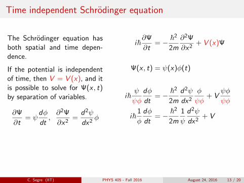
Time independent Schrodinger equation
The Schrodinger equation hasboth spatial and time depen-dence.
If the potential is independentof time, then V = V (x), and itis possible to solve for Ψ(x , t)by separation of variables.
∂Ψ
∂t= ψ
dφ
dt,∂2Ψ
∂x2=
d2ψ
dx2φ
This can be solved only if eachside of the separable equation isa constant, E .
i~∂Ψ
∂t= − ~2
2m
∂2Ψ
∂x2+ V (x)Ψ
Ψ(x , t) = ψ(x)φ(t)
i~ψ
ψφ
dφ
dt= − ~2
2m
d2ψ
dx2
φ
ψφ+ V
ψφ
ψφ
i~1
φ
dφ
dt= − ~2
2m
1
ψ
d2ψ
dx2+ V
We will now proceed to solve each ofthe two ordinary differential equationswhich make up the time-independentSchrodinger equation
C. Segre (IIT) PHYS 405 - Fall 2016 August 24, 2016 13 / 20
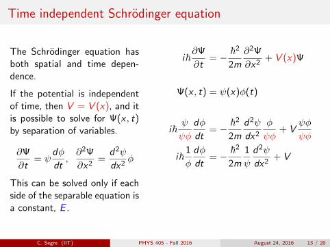
Time independent Schrodinger equation
The Schrodinger equation hasboth spatial and time depen-dence.
If the potential is independentof time, then V = V (x), and itis possible to solve for Ψ(x , t)by separation of variables.
∂Ψ
∂t= ψ
dφ
dt,∂2Ψ
∂x2=
d2ψ
dx2φ
This can be solved only if eachside of the separable equation isa constant, E .
i~∂Ψ
∂t= − ~2
2m
∂2Ψ
∂x2+ V (x)Ψ
Ψ(x , t) = ψ(x)φ(t)
i~ψ
ψφ
dφ
dt= − ~2
2m
d2ψ
dx2
φ
ψφ+ V
ψφ
ψφ
i~1
φ
dφ
dt= − ~2
2m
1
ψ
d2ψ
dx2+ V
We will now proceed to solve each ofthe two ordinary differential equationswhich make up the time-independentSchrodinger equation
C. Segre (IIT) PHYS 405 - Fall 2016 August 24, 2016 13 / 20
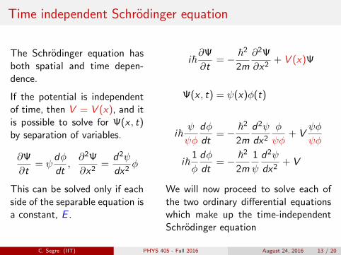
Time independent Schrodinger equation
The Schrodinger equation hasboth spatial and time depen-dence.
If the potential is independentof time, then V = V (x), and itis possible to solve for Ψ(x , t)by separation of variables.
∂Ψ
∂t= ψ
dφ
dt,∂2Ψ
∂x2=
d2ψ
dx2φ
This can be solved only if eachside of the separable equation isa constant, E .
i~∂Ψ
∂t= − ~2
2m
∂2Ψ
∂x2+ V (x)Ψ
Ψ(x , t) = ψ(x)φ(t)
i~ψ
ψφ
dφ
dt= − ~2
2m
d2ψ
dx2
φ
ψφ+ V
ψφ
ψφ
i~1
φ
dφ
dt= − ~2
2m
1
ψ
d2ψ
dx2+ V
We will now proceed to solve each ofthe two ordinary differential equationswhich make up the time-independentSchrodinger equation
C. Segre (IIT) PHYS 405 - Fall 2016 August 24, 2016 13 / 20
Time-dependent equation
First solve the time-dependentportion since the spatial portionwill depend on the details of thepotential energy, V (x).
The solution must be of theform , but the constant can befolded into the spatial solutionψ(x)
The total wavefunction de-pends on t, but the probabilitydensity does not.
Expectation values are also in-dependent of time
i~1
φ
dφ
dt= E
dφ
dt= − iE
~φ
φ = ��Ce−iEt/~
Ψ(x , t) = ψ(x)e−iEt/~
|Ψ(x , t)|2 = ψ∗����e+iEt/~ψ����
e−iEt/~
= ψ∗ψ = |ψ(x)|2
〈Q(x , p)〉 =
∫ψ∗����
e+iEt/~Qψ����e−iEt/~dx
=
∫ψ∗Qψdx
C. Segre (IIT) PHYS 405 - Fall 2016 August 24, 2016 14 / 20
Time-dependent equation
First solve the time-dependentportion since the spatial portionwill depend on the details of thepotential energy, V (x).
The solution must be of theform
, but the constant can befolded into the spatial solutionψ(x)
The total wavefunction de-pends on t, but the probabilitydensity does not.
Expectation values are also in-dependent of time
i~1
φ
dφ
dt= E
dφ
dt= − iE
~φ
φ = Ce−iEt/~
Ψ(x , t) = ψ(x)e−iEt/~
|Ψ(x , t)|2 = ψ∗����e+iEt/~ψ����
e−iEt/~
= ψ∗ψ = |ψ(x)|2
〈Q(x , p)〉 =
∫ψ∗����
e+iEt/~Qψ����e−iEt/~dx
=
∫ψ∗Qψdx
C. Segre (IIT) PHYS 405 - Fall 2016 August 24, 2016 14 / 20
Time-dependent equation
First solve the time-dependentportion since the spatial portionwill depend on the details of thepotential energy, V (x).
The solution must be of theform , but the constant can befolded into the spatial solutionψ(x)
The total wavefunction de-pends on t, but the probabilitydensity does not.
Expectation values are also in-dependent of time
i~1
φ
dφ
dt= E
dφ
dt= − iE
~φ
φ = ��Ce−iEt/~
Ψ(x , t) = ψ(x)e−iEt/~
|Ψ(x , t)|2 = ψ∗����e+iEt/~ψ����
e−iEt/~
= ψ∗ψ = |ψ(x)|2
〈Q(x , p)〉 =
∫ψ∗����
e+iEt/~Qψ����e−iEt/~dx
=
∫ψ∗Qψdx
C. Segre (IIT) PHYS 405 - Fall 2016 August 24, 2016 14 / 20
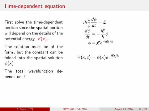
Time-dependent equation
First solve the time-dependentportion since the spatial portionwill depend on the details of thepotential energy, V (x).
The solution must be of theform , but the constant can befolded into the spatial solutionψ(x)
The total wavefunction de-pends on t
, but the probabilitydensity does not.
Expectation values are also in-dependent of time
i~1
φ
dφ
dt= E
dφ
dt= − iE
~φ
φ = ��Ce−iEt/~
Ψ(x , t) = ψ(x)e−iEt/~
|Ψ(x , t)|2 = ψ∗����e+iEt/~ψ����
e−iEt/~
= ψ∗ψ = |ψ(x)|2
〈Q(x , p)〉 =
∫ψ∗����
e+iEt/~Qψ����e−iEt/~dx
=
∫ψ∗Qψdx
C. Segre (IIT) PHYS 405 - Fall 2016 August 24, 2016 14 / 20
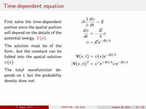
Time-dependent equation
First solve the time-dependentportion since the spatial portionwill depend on the details of thepotential energy, V (x).
The solution must be of theform , but the constant can befolded into the spatial solutionψ(x)
The total wavefunction de-pends on t, but the probabilitydensity does not.
Expectation values are also in-dependent of time
i~1
φ
dφ
dt= E
dφ
dt= − iE
~φ
φ = ��Ce−iEt/~
Ψ(x , t) = ψ(x)e−iEt/~
|Ψ(x , t)|2 = ψ∗e+iEt/~ψe−iEt/~
= ψ∗ψ = |ψ(x)|2
〈Q(x , p)〉 =
∫ψ∗����
e+iEt/~Qψ����e−iEt/~dx
=
∫ψ∗Qψdx
C. Segre (IIT) PHYS 405 - Fall 2016 August 24, 2016 14 / 20
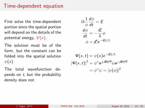
Time-dependent equation
First solve the time-dependentportion since the spatial portionwill depend on the details of thepotential energy, V (x).
The solution must be of theform , but the constant can befolded into the spatial solutionψ(x)
The total wavefunction de-pends on t, but the probabilitydensity does not.
Expectation values are also in-dependent of time
i~1
φ
dφ
dt= E
dφ
dt= − iE
~φ
φ = ��Ce−iEt/~
Ψ(x , t) = ψ(x)e−iEt/~
|Ψ(x , t)|2 = ψ∗����e+iEt/~ψ����
e−iEt/~
= ψ∗ψ = |ψ(x)|2
〈Q(x , p)〉 =
∫ψ∗����
e+iEt/~Qψ����e−iEt/~dx
=
∫ψ∗Qψdx
C. Segre (IIT) PHYS 405 - Fall 2016 August 24, 2016 14 / 20
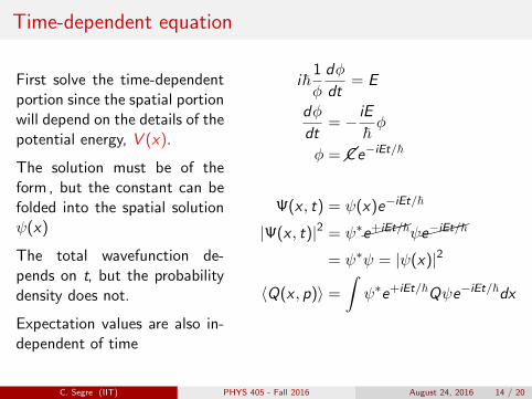
Time-dependent equation
First solve the time-dependentportion since the spatial portionwill depend on the details of thepotential energy, V (x).
The solution must be of theform , but the constant can befolded into the spatial solutionψ(x)
The total wavefunction de-pends on t, but the probabilitydensity does not.
Expectation values are also in-dependent of time
i~1
φ
dφ
dt= E
dφ
dt= − iE
~φ
φ = ��Ce−iEt/~
Ψ(x , t) = ψ(x)e−iEt/~
|Ψ(x , t)|2 = ψ∗����e+iEt/~ψ����
e−iEt/~
= ψ∗ψ = |ψ(x)|2
〈Q(x , p)〉 =
∫ψ∗e+iEt/~Qψe−iEt/~dx
=
∫ψ∗Qψdx
C. Segre (IIT) PHYS 405 - Fall 2016 August 24, 2016 14 / 20
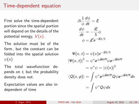
Time-dependent equation
First solve the time-dependentportion since the spatial portionwill depend on the details of thepotential energy, V (x).
The solution must be of theform , but the constant can befolded into the spatial solutionψ(x)
The total wavefunction de-pends on t, but the probabilitydensity does not.
Expectation values are also in-dependent of time
i~1
φ
dφ
dt= E
dφ
dt= − iE
~φ
φ = ��Ce−iEt/~
Ψ(x , t) = ψ(x)e−iEt/~
|Ψ(x , t)|2 = ψ∗����e+iEt/~ψ����
e−iEt/~
= ψ∗ψ = |ψ(x)|2
〈Q(x , p)〉 =
∫ψ∗����
e+iEt/~Qψ����e−iEt/~dx
=
∫ψ∗Qψdx
C. Segre (IIT) PHYS 405 - Fall 2016 August 24, 2016 14 / 20
Properties of stationary states
Stationary states have a definite en-ergy E .
The left side is simply thequantum operator corresponding tothe classical Hamiltonian
H(x , p) =p2
2m+ V (x)
the Schrodinger equation
the expectation value of the energy
the variance of the energy
− ~2
2m
d2
dx2ψ + Vψ = Eψ
H = − ~2
2m
d2
dx2+ V (x)
Hψ = Eψ
〈H〉 =
∫ψ∗Hψdx
= E
∫ψ∗ψdx = E
σ2H =
⟨H2⟩−⟨H⟩2
= E 2 − E 2 = 0
C. Segre (IIT) PHYS 405 - Fall 2016 August 24, 2016 15 / 20
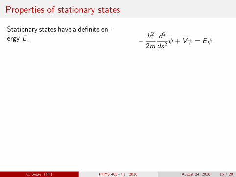
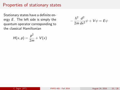
Properties of stationary states
Stationary states have a definite en-ergy E . The left side is simply thequantum operator corresponding tothe classical Hamiltonian
H(x , p) =p2
2m+ V (x)
the Schrodinger equation
the expectation value of the energy
the variance of the energy
− ~2
2m
d2
dx2ψ + Vψ = Eψ
H = − ~2
2m
d2
dx2+ V (x)
Hψ = Eψ
〈H〉 =
∫ψ∗Hψdx
= E
∫ψ∗ψdx = E
σ2H =
⟨H2⟩−⟨H⟩2
= E 2 − E 2 = 0
C. Segre (IIT) PHYS 405 - Fall 2016 August 24, 2016 15 / 20
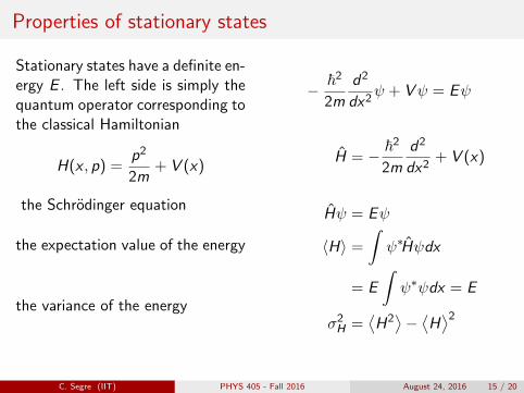
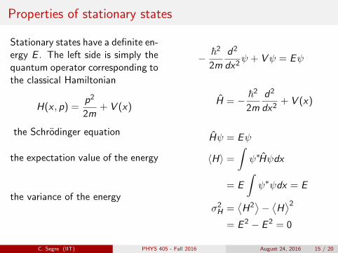
Constructing the time-dependent solution
Each spatial solutions, the station-ary states, will have a specific en-ergy and there are an infinite num-ber of such solutions.
Thus, a full time-dependent solu-tion can be obtained by a linearcombination of time-independentwave functions.
Ψ1(x , t) = ψ1(x)e−iE1t/~
Ψ2(x , t) = ψ2(x)e−iE2t/~
...
Ψn(x , t) = ψn(x)e−iEnt/~
Ψ(x , t) =∞∑n=1
cnψne−iEnt/~
The general solution does not have time-independent expectation values,nor does it have zero variance for the expectation value of the energy
We generally leave the time-dependent portion as an implicit part of thesolution.
C. Segre (IIT) PHYS 405 - Fall 2016 August 24, 2016 16 / 20
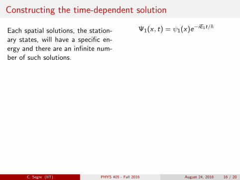
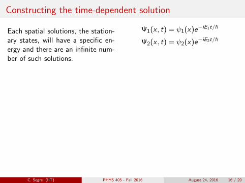
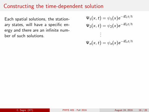
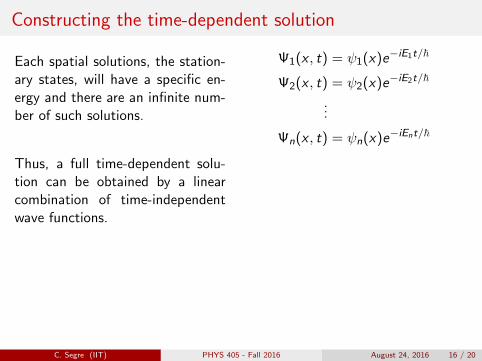
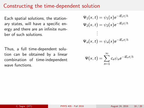
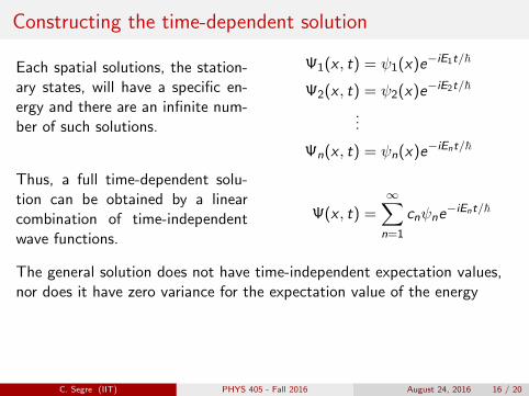
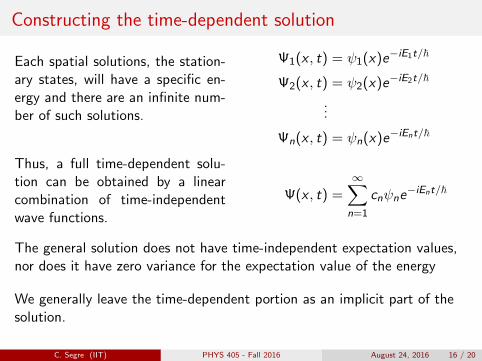
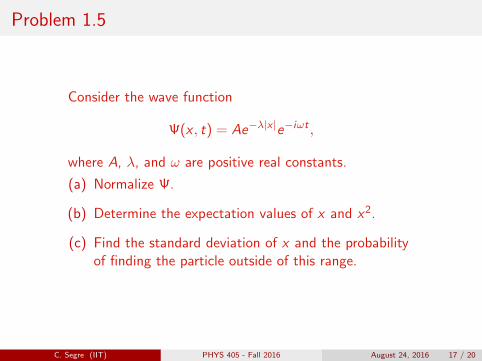
Problem 1.5
Consider the wave function
Ψ(x , t) = Ae−λ|x |e−iωt ,
where A, λ, and ω are positive real constants.
(a) Normalize Ψ.
(b) Determine the expectation values of x and x2.
(c) Find the standard deviation of x and the probabilityof finding the particle outside of this range.
C. Segre (IIT) PHYS 405 - Fall 2016 August 24, 2016 17 / 20

Problem 1.5 - part (a)
The normalization integral is
1 =
∫ψ∗ψ dx = A2
∫ ∞−∞
e−λ|x |���e iωte−λ|x |���e−iωt dx = A2
∫ ∞−∞
e−2λ|x | dx
= A2
(∫ 0
−∞e+2λx dx
+
∫ ∞0
e−2λx dx
)break this into two integrals
= A2
(1
2λe2λx
∣∣∣0−∞
− 1
2λe−2λx
∣∣∣∞0
)= A2
(1
2λ+
1
2λ
)=
A2
λ
A =√λ
So the normalized wave function is
Ψ(x , t) =√λe−λ|x |e−iωt
C. Segre (IIT) PHYS 405 - Fall 2016 August 24, 2016 18 / 20
Problem 1.5 - part (a)
The normalization integral is
1 =
∫ψ∗ψ dx
= A2
∫ ∞−∞
e−λ|x |���e iωte−λ|x |���e−iωt dx = A2
∫ ∞−∞
e−2λ|x | dx
= A2
(∫ 0
−∞e+2λx dx
+
∫ ∞0
e−2λx dx
)break this into two integrals
= A2
(1
2λe2λx
∣∣∣0−∞
− 1
2λe−2λx
∣∣∣∞0
)= A2
(1
2λ+
1
2λ
)=
A2
λ
A =√λ
So the normalized wave function is
Ψ(x , t) =√λe−λ|x |e−iωt
C. Segre (IIT) PHYS 405 - Fall 2016 August 24, 2016 18 / 20
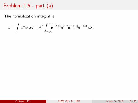
Problem 1.5 - part (a)
The normalization integral is
1 =
∫ψ∗ψ dx = A2
∫ ∞−∞
e−λ|x |e iωte−λ|x |e−iωt dx
= A2
∫ ∞−∞
e−2λ|x | dx
= A2
(∫ 0
−∞e+2λx dx
+
∫ ∞0
e−2λx dx
)break this into two integrals
= A2
(1
2λe2λx
∣∣∣0−∞
− 1
2λe−2λx
∣∣∣∞0
)= A2
(1
2λ+
1
2λ
)=
A2
λ
A =√λ
So the normalized wave function is
Ψ(x , t) =√λe−λ|x |e−iωt
C. Segre (IIT) PHYS 405 - Fall 2016 August 24, 2016 18 / 20
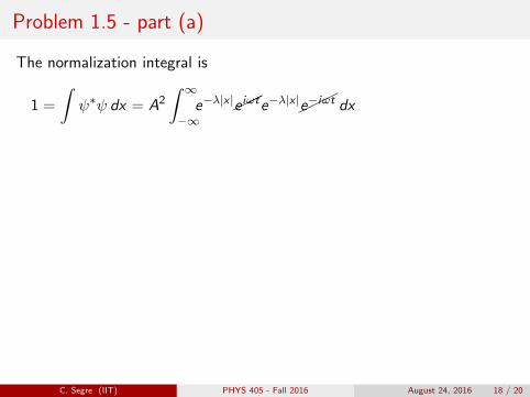
Problem 1.5 - part (a)
The normalization integral is
1 =
∫ψ∗ψ dx = A2
∫ ∞−∞
e−λ|x |���e iωte−λ|x |���e−iωt dx
= A2
∫ ∞−∞
e−2λ|x | dx
= A2
(∫ 0
−∞e+2λx dx
+
∫ ∞0
e−2λx dx
)break this into two integrals
= A2
(1
2λe2λx
∣∣∣0−∞
− 1
2λe−2λx
∣∣∣∞0
)= A2
(1
2λ+
1
2λ
)=
A2
λ
A =√λ
So the normalized wave function is
Ψ(x , t) =√λe−λ|x |e−iωt
C. Segre (IIT) PHYS 405 - Fall 2016 August 24, 2016 18 / 20
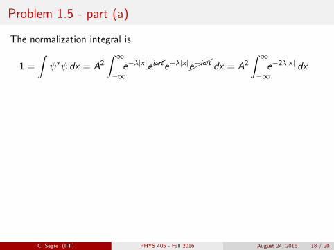
Problem 1.5 - part (a)
The normalization integral is
1 =
∫ψ∗ψ dx = A2
∫ ∞−∞
e−λ|x |���e iωte−λ|x |���e−iωt dx = A2
∫ ∞−∞
e−2λ|x | dx
= A2
(∫ 0
−∞e+2λx dx
+
∫ ∞0
e−2λx dx
)break this into two integrals
= A2
(1
2λe2λx
∣∣∣0−∞
− 1
2λe−2λx
∣∣∣∞0
)= A2
(1
2λ+
1
2λ
)=
A2
λ
A =√λ
So the normalized wave function is
Ψ(x , t) =√λe−λ|x |e−iωt
C. Segre (IIT) PHYS 405 - Fall 2016 August 24, 2016 18 / 20
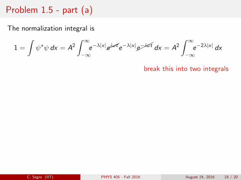
Problem 1.5 - part (a)
The normalization integral is
1 =
∫ψ∗ψ dx = A2
∫ ∞−∞
e−λ|x |���e iωte−λ|x |���e−iωt dx = A2
∫ ∞−∞
e−2λ|x | dx
= A2
(∫ 0
−∞e+2λx dx
+
∫ ∞0
e−2λx dx
)
break this into two integrals
= A2
(1
2λe2λx
∣∣∣0−∞
− 1
2λe−2λx
∣∣∣∞0
)= A2
(1
2λ+
1
2λ
)=
A2
λ
A =√λ
So the normalized wave function is
Ψ(x , t) =√λe−λ|x |e−iωt
C. Segre (IIT) PHYS 405 - Fall 2016 August 24, 2016 18 / 20
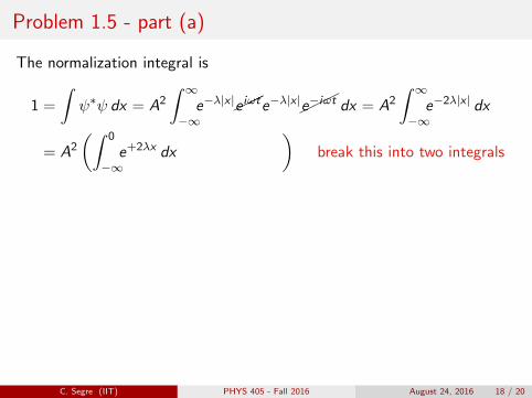
Problem 1.5 - part (a)
The normalization integral is
1 =
∫ψ∗ψ dx = A2
∫ ∞−∞
e−λ|x |���e iωte−λ|x |���e−iωt dx = A2
∫ ∞−∞
e−2λ|x | dx
= A2
(∫ 0
−∞e+2λx dx
+
∫ ∞0
e−2λx dx
)break this into two integrals
= A2
(1
2λe2λx
∣∣∣0−∞
− 1
2λe−2λx
∣∣∣∞0
)= A2
(1
2λ+
1
2λ
)=
A2
λ
A =√λ
So the normalized wave function is
Ψ(x , t) =√λe−λ|x |e−iωt
C. Segre (IIT) PHYS 405 - Fall 2016 August 24, 2016 18 / 20
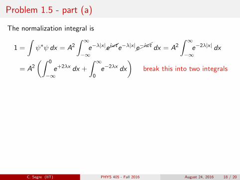
Problem 1.5 - part (a)
The normalization integral is
1 =
∫ψ∗ψ dx = A2
∫ ∞−∞
e−λ|x |���e iωte−λ|x |���e−iωt dx = A2
∫ ∞−∞
e−2λ|x | dx
= A2
(∫ 0
−∞e+2λx dx +
∫ ∞0
e−2λx dx
)break this into two integrals
= A2
(1
2λe2λx
∣∣∣0−∞
− 1
2λe−2λx
∣∣∣∞0
)= A2
(1
2λ+
1
2λ
)=
A2
λ
A =√λ
So the normalized wave function is
Ψ(x , t) =√λe−λ|x |e−iωt
C. Segre (IIT) PHYS 405 - Fall 2016 August 24, 2016 18 / 20
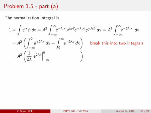
Problem 1.5 - part (a)
The normalization integral is
1 =
∫ψ∗ψ dx = A2
∫ ∞−∞
e−λ|x |���e iωte−λ|x |���e−iωt dx = A2
∫ ∞−∞
e−2λ|x | dx
= A2
(∫ 0
−∞e+2λx dx +
∫ ∞0
e−2λx dx
)break this into two integrals
= A2
(1
2λe2λx
∣∣∣0−∞
− 1
2λe−2λx
∣∣∣∞0
)
= A2
(1
2λ+
1
2λ
)=
A2
λ
A =√λ
So the normalized wave function is
Ψ(x , t) =√λe−λ|x |e−iωt
C. Segre (IIT) PHYS 405 - Fall 2016 August 24, 2016 18 / 20
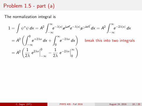
Problem 1.5 - part (a)
The normalization integral is
1 =
∫ψ∗ψ dx = A2
∫ ∞−∞
e−λ|x |���e iωte−λ|x |���e−iωt dx = A2
∫ ∞−∞
e−2λ|x | dx
= A2
(∫ 0
−∞e+2λx dx +
∫ ∞0
e−2λx dx
)break this into two integrals
= A2
(1
2λe2λx
∣∣∣0−∞− 1
2λe−2λx
∣∣∣∞0
)
= A2
(1
2λ+
1
2λ
)=
A2
λ
A =√λ
So the normalized wave function is
Ψ(x , t) =√λe−λ|x |e−iωt
C. Segre (IIT) PHYS 405 - Fall 2016 August 24, 2016 18 / 20
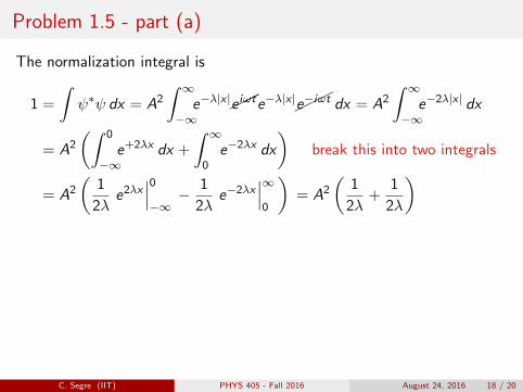
Problem 1.5 - part (a)
The normalization integral is
1 =
∫ψ∗ψ dx = A2
∫ ∞−∞
e−λ|x |���e iωte−λ|x |���e−iωt dx = A2
∫ ∞−∞
e−2λ|x | dx
= A2
(∫ 0
−∞e+2λx dx +
∫ ∞0
e−2λx dx
)break this into two integrals
= A2
(1
2λe2λx
∣∣∣0−∞− 1
2λe−2λx
∣∣∣∞0
)= A2
(1
2λ+
1
2λ
)
=A2
λ
A =√λ
So the normalized wave function is
Ψ(x , t) =√λe−λ|x |e−iωt
C. Segre (IIT) PHYS 405 - Fall 2016 August 24, 2016 18 / 20
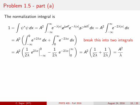
Problem 1.5 - part (a)
The normalization integral is
1 =
∫ψ∗ψ dx = A2
∫ ∞−∞
e−λ|x |���e iωte−λ|x |���e−iωt dx = A2
∫ ∞−∞
e−2λ|x | dx
= A2
(∫ 0
−∞e+2λx dx +
∫ ∞0
e−2λx dx
)break this into two integrals
= A2
(1
2λe2λx
∣∣∣0−∞− 1
2λe−2λx
∣∣∣∞0
)= A2
(1
2λ+
1
2λ
)=
A2
λ
A =√λ
So the normalized wave function is
Ψ(x , t) =√λe−λ|x |e−iωt
C. Segre (IIT) PHYS 405 - Fall 2016 August 24, 2016 18 / 20
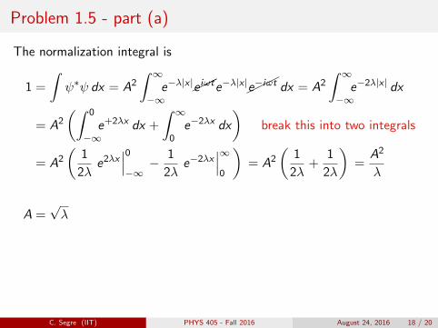
Problem 1.5 - part (a)
The normalization integral is
1 =
∫ψ∗ψ dx = A2
∫ ∞−∞
e−λ|x |���e iωte−λ|x |���e−iωt dx = A2
∫ ∞−∞
e−2λ|x | dx
= A2
(∫ 0
−∞e+2λx dx +
∫ ∞0
e−2λx dx
)break this into two integrals
= A2
(1
2λe2λx
∣∣∣0−∞− 1
2λe−2λx
∣∣∣∞0
)= A2
(1
2λ+
1
2λ
)=
A2
λ
A =√λ
So the normalized wave function is
Ψ(x , t) =√λe−λ|x |e−iωt
C. Segre (IIT) PHYS 405 - Fall 2016 August 24, 2016 18 / 20
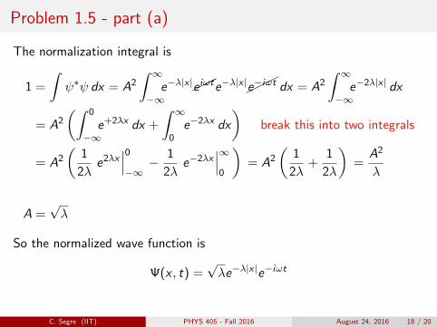
Problem 1.5 - part (a)
The normalization integral is
1 =
∫ψ∗ψ dx = A2
∫ ∞−∞
e−λ|x |���e iωte−λ|x |���e−iωt dx = A2
∫ ∞−∞
e−2λ|x | dx
= A2
(∫ 0
−∞e+2λx dx +
∫ ∞0
e−2λx dx
)break this into two integrals
= A2
(1
2λe2λx
∣∣∣0−∞− 1
2λe−2λx
∣∣∣∞0
)= A2
(1
2λ+
1
2λ
)=
A2
λ
A =√λ
So the normalized wave function is
Ψ(x , t) =√λe−λ|x |e−iωt
C. Segre (IIT) PHYS 405 - Fall 2016 August 24, 2016 18 / 20
Problem 1.5 - part (b)
The expectation value of x is
〈x〉 = λ
∫ ∞−∞
xe−2λ|x | dx
= 0
this vanishes due to an odd integrand. The expectation value of x2 is⟨x2⟩
= λ
(∫ 0
−∞x2e+2λx dx +
∫ ∞0
x2e−2λx dx
)= 2λ
∫ ∞0
x2e−2λx dx
this can be solved applying integration by parts twice, first using
u = x2, du = 2x dx , dv = e−2λxdx , v = − 1
2λe−2λx
⟨x2⟩
= 2λ
(−��
����x2e−2λx
2λ
∣∣∣∣∞0
+1
λ
∫ ∞0
xe−2λx dx
)= +2
∫ ∞0
x e−2λx dx
and with u = x , du = dx for the second
⟨x2⟩
= 2
(−��
���xe−2λx
2λ
∣∣∣∣∞0
+1
2λ
∫ ∞0
e−2λx dx
)= +
1
λ
∫ ∞0
e−2λx dx =1
2λ2
C. Segre (IIT) PHYS 405 - Fall 2016 August 24, 2016 19 / 20
Problem 1.5 - part (b)
The expectation value of x is
〈x〉 = λ
∫ ∞−∞
xe−2λ|x | dx
= 0
this vanishes due to an odd integrand.
The expectation value of x2 is⟨x2⟩
= λ
(∫ 0
−∞x2e+2λx dx +
∫ ∞0
x2e−2λx dx
)= 2λ
∫ ∞0
x2e−2λx dx
this can be solved applying integration by parts twice, first using
u = x2, du = 2x dx , dv = e−2λxdx , v = − 1
2λe−2λx
⟨x2⟩
= 2λ
(−��
����x2e−2λx
2λ
∣∣∣∣∞0
+1
λ
∫ ∞0
xe−2λx dx
)= +2
∫ ∞0
x e−2λx dx
and with u = x , du = dx for the second
⟨x2⟩
= 2
(−��
���xe−2λx
2λ
∣∣∣∣∞0
+1
2λ
∫ ∞0
e−2λx dx
)= +
1
λ
∫ ∞0
e−2λx dx =1
2λ2
C. Segre (IIT) PHYS 405 - Fall 2016 August 24, 2016 19 / 20
Problem 1.5 - part (b)
The expectation value of x is
〈x〉 = λ
∫ ∞−∞
xe−2λ|x | dx = 0
this vanishes due to an odd integrand.
The expectation value of x2 is⟨x2⟩
= λ
(∫ 0
−∞x2e+2λx dx +
∫ ∞0
x2e−2λx dx
)= 2λ
∫ ∞0
x2e−2λx dx
this can be solved applying integration by parts twice, first using
u = x2, du = 2x dx , dv = e−2λxdx , v = − 1
2λe−2λx
⟨x2⟩
= 2λ
(−��
����x2e−2λx
2λ
∣∣∣∣∞0
+1
λ
∫ ∞0
xe−2λx dx
)= +2
∫ ∞0
x e−2λx dx
and with u = x , du = dx for the second
⟨x2⟩
= 2
(−��
���xe−2λx
2λ
∣∣∣∣∞0
+1
2λ
∫ ∞0
e−2λx dx
)= +
1
λ
∫ ∞0
e−2λx dx =1
2λ2
C. Segre (IIT) PHYS 405 - Fall 2016 August 24, 2016 19 / 20
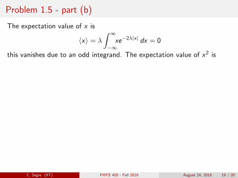
Problem 1.5 - part (b)
The expectation value of x is
〈x〉 = λ
∫ ∞−∞
xe−2λ|x | dx = 0
this vanishes due to an odd integrand. The expectation value of x2 is
⟨x2⟩
= λ
(∫ 0
−∞x2e+2λx dx +
∫ ∞0
x2e−2λx dx
)= 2λ
∫ ∞0
x2e−2λx dx
this can be solved applying integration by parts twice, first using
u = x2, du = 2x dx , dv = e−2λxdx , v = − 1
2λe−2λx
⟨x2⟩
= 2λ
(−��
����x2e−2λx
2λ
∣∣∣∣∞0
+1
λ
∫ ∞0
xe−2λx dx
)= +2
∫ ∞0
x e−2λx dx
and with u = x , du = dx for the second
⟨x2⟩
= 2
(−��
���xe−2λx
2λ
∣∣∣∣∞0
+1
2λ
∫ ∞0
e−2λx dx
)= +
1
λ
∫ ∞0
e−2λx dx =1
2λ2
C. Segre (IIT) PHYS 405 - Fall 2016 August 24, 2016 19 / 20
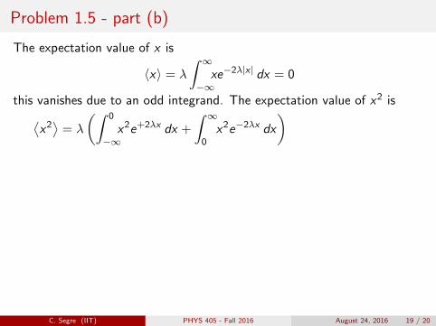
Problem 1.5 - part (b)
The expectation value of x is
〈x〉 = λ
∫ ∞−∞
xe−2λ|x | dx = 0
this vanishes due to an odd integrand. The expectation value of x2 is⟨x2⟩
= λ
(∫ 0
−∞x2e+2λx dx +
∫ ∞0
x2e−2λx dx
)
= 2λ
∫ ∞0
x2e−2λx dx
this can be solved applying integration by parts twice, first using
u = x2, du = 2x dx , dv = e−2λxdx , v = − 1
2λe−2λx
⟨x2⟩
= 2λ
(−��
����x2e−2λx
2λ
∣∣∣∣∞0
+1
λ
∫ ∞0
xe−2λx dx
)= +2
∫ ∞0
x e−2λx dx
and with u = x , du = dx for the second
⟨x2⟩
= 2
(−��
���xe−2λx
2λ
∣∣∣∣∞0
+1
2λ
∫ ∞0
e−2λx dx
)= +
1
λ
∫ ∞0
e−2λx dx =1
2λ2
C. Segre (IIT) PHYS 405 - Fall 2016 August 24, 2016 19 / 20
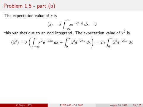
Problem 1.5 - part (b)
The expectation value of x is
〈x〉 = λ
∫ ∞−∞
xe−2λ|x | dx = 0
this vanishes due to an odd integrand. The expectation value of x2 is⟨x2⟩
= λ
(∫ 0
−∞x2e+2λx dx +
∫ ∞0
x2e−2λx dx
)= 2λ
∫ ∞0
x2e−2λx dx
this can be solved applying integration by parts twice, first using
u = x2, du = 2x dx , dv = e−2λxdx , v = − 1
2λe−2λx
⟨x2⟩
= 2λ
(−��
����x2e−2λx
2λ
∣∣∣∣∞0
+1
λ
∫ ∞0
xe−2λx dx
)= +2
∫ ∞0
x e−2λx dx
and with u = x , du = dx for the second
⟨x2⟩
= 2
(−��
���xe−2λx
2λ
∣∣∣∣∞0
+1
2λ
∫ ∞0
e−2λx dx
)= +
1
λ
∫ ∞0
e−2λx dx =1
2λ2
C. Segre (IIT) PHYS 405 - Fall 2016 August 24, 2016 19 / 20
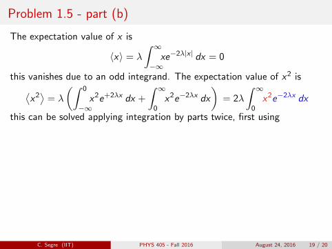
Problem 1.5 - part (b)
The expectation value of x is
〈x〉 = λ
∫ ∞−∞
xe−2λ|x | dx = 0
this vanishes due to an odd integrand. The expectation value of x2 is⟨x2⟩
= λ
(∫ 0
−∞x2e+2λx dx +
∫ ∞0
x2e−2λx dx
)= 2λ
∫ ∞0
x2e−2λx dx
this can be solved applying integration by parts twice, first using
u = x2, du = 2x dx , dv = e−2λxdx , v = − 1
2λe−2λx
⟨x2⟩
= 2λ
(−��
����x2e−2λx
2λ
∣∣∣∣∞0
+1
λ
∫ ∞0
xe−2λx dx
)= +2
∫ ∞0
x e−2λx dx
and with u = x , du = dx for the second
⟨x2⟩
= 2
(−��
���xe−2λx
2λ
∣∣∣∣∞0
+1
2λ
∫ ∞0
e−2λx dx
)= +
1
λ
∫ ∞0
e−2λx dx =1
2λ2
C. Segre (IIT) PHYS 405 - Fall 2016 August 24, 2016 19 / 20
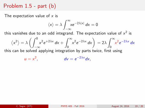
Problem 1.5 - part (b)
The expectation value of x is
〈x〉 = λ
∫ ∞−∞
xe−2λ|x | dx = 0
this vanishes due to an odd integrand. The expectation value of x2 is⟨x2⟩
= λ
(∫ 0
−∞x2e+2λx dx +
∫ ∞0
x2e−2λx dx
)= 2λ
∫ ∞0
x2e−2λx dx
this can be solved applying integration by parts twice, first using
u = x2,
du = 2x dx ,
dv = e−2λxdx ,
v = − 1
2λe−2λx
⟨x2⟩
= 2λ
(−��
����x2e−2λx
2λ
∣∣∣∣∞0
+1
λ
∫ ∞0
xe−2λx dx
)= +2
∫ ∞0
x e−2λx dx
and with u = x , du = dx for the second
⟨x2⟩
= 2
(−��
���xe−2λx
2λ
∣∣∣∣∞0
+1
2λ
∫ ∞0
e−2λx dx
)= +
1
λ
∫ ∞0
e−2λx dx =1
2λ2
C. Segre (IIT) PHYS 405 - Fall 2016 August 24, 2016 19 / 20
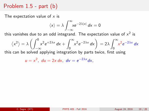
Problem 1.5 - part (b)
The expectation value of x is
〈x〉 = λ
∫ ∞−∞
xe−2λ|x | dx = 0
this vanishes due to an odd integrand. The expectation value of x2 is⟨x2⟩
= λ
(∫ 0
−∞x2e+2λx dx +
∫ ∞0
x2e−2λx dx
)= 2λ
∫ ∞0
x2e−2λx dx
this can be solved applying integration by parts twice, first using
u = x2, du = 2x dx , dv = e−2λxdx ,
v = − 1
2λe−2λx
⟨x2⟩
= 2λ
(−��
����x2e−2λx
2λ
∣∣∣∣∞0
+1
λ
∫ ∞0
xe−2λx dx
)= +2
∫ ∞0
x e−2λx dx
and with u = x , du = dx for the second
⟨x2⟩
= 2
(−��
���xe−2λx
2λ
∣∣∣∣∞0
+1
2λ
∫ ∞0
e−2λx dx
)= +
1
λ
∫ ∞0
e−2λx dx =1
2λ2
C. Segre (IIT) PHYS 405 - Fall 2016 August 24, 2016 19 / 20
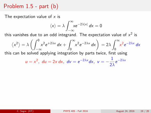
Problem 1.5 - part (b)
The expectation value of x is
〈x〉 = λ
∫ ∞−∞
xe−2λ|x | dx = 0
this vanishes due to an odd integrand. The expectation value of x2 is⟨x2⟩
= λ
(∫ 0
−∞x2e+2λx dx +
∫ ∞0
x2e−2λx dx
)= 2λ
∫ ∞0
x2e−2λx dx
this can be solved applying integration by parts twice, first using
u = x2, du = 2x dx , dv = e−2λxdx , v = − 1
2λe−2λx
⟨x2⟩
= 2λ
(−��
����x2e−2λx
2λ
∣∣∣∣∞0
+1
λ
∫ ∞0
xe−2λx dx
)= +2
∫ ∞0
x e−2λx dx
and with u = x , du = dx for the second
⟨x2⟩
= 2
(−��
���xe−2λx
2λ
∣∣∣∣∞0
+1
2λ
∫ ∞0
e−2λx dx
)= +
1
λ
∫ ∞0
e−2λx dx =1
2λ2
C. Segre (IIT) PHYS 405 - Fall 2016 August 24, 2016 19 / 20
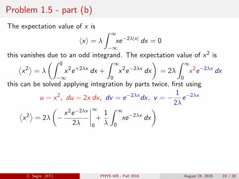
Problem 1.5 - part (b)
The expectation value of x is
〈x〉 = λ
∫ ∞−∞
xe−2λ|x | dx = 0
this vanishes due to an odd integrand. The expectation value of x2 is⟨x2⟩
= λ
(∫ 0
−∞x2e+2λx dx +
∫ ∞0
x2e−2λx dx
)= 2λ
∫ ∞0
x2e−2λx dx
this can be solved applying integration by parts twice, first using
u = x2, du = 2x dx , dv = e−2λxdx , v = − 1
2λe−2λx
⟨x2⟩
= 2λ
(− x2e−2λx
2λ
∣∣∣∣∞0
+1
λ
∫ ∞0
xe−2λx dx
)
= +2
∫ ∞0
x e−2λx dx
and with u = x , du = dx for the second
⟨x2⟩
= 2
(−�
����xe−2λx
2λ
∣∣∣∣∞0
+1
2λ
∫ ∞0
e−2λx dx
)= +
1
λ
∫ ∞0
e−2λx dx =1
2λ2
C. Segre (IIT) PHYS 405 - Fall 2016 August 24, 2016 19 / 20
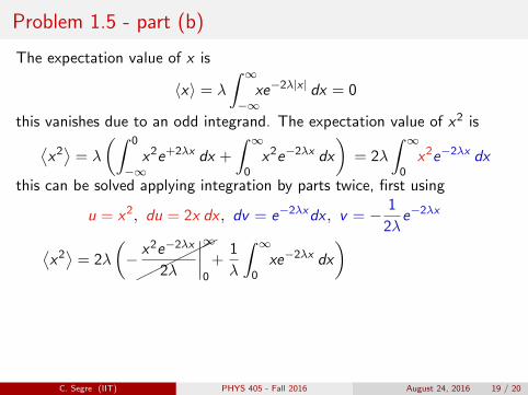
Problem 1.5 - part (b)
The expectation value of x is
〈x〉 = λ
∫ ∞−∞
xe−2λ|x | dx = 0
this vanishes due to an odd integrand. The expectation value of x2 is⟨x2⟩
= λ
(∫ 0
−∞x2e+2λx dx +
∫ ∞0
x2e−2λx dx
)= 2λ
∫ ∞0
x2e−2λx dx
this can be solved applying integration by parts twice, first using
u = x2, du = 2x dx , dv = e−2λxdx , v = − 1
2λe−2λx
⟨x2⟩
= 2λ
(−��
����x2e−2λx
2λ
∣∣∣∣∞0
+1
λ
∫ ∞0
xe−2λx dx
)
= +2
∫ ∞0
x e−2λx dx
and with u = x , du = dx for the second
⟨x2⟩
= 2
(−��
���xe−2λx
2λ
∣∣∣∣∞0
+1
2λ
∫ ∞0
e−2λx dx
)= +
1
λ
∫ ∞0
e−2λx dx =1
2λ2
C. Segre (IIT) PHYS 405 - Fall 2016 August 24, 2016 19 / 20
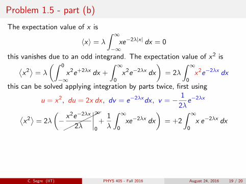
Problem 1.5 - part (b)
The expectation value of x is
〈x〉 = λ
∫ ∞−∞
xe−2λ|x | dx = 0
this vanishes due to an odd integrand. The expectation value of x2 is⟨x2⟩
= λ
(∫ 0
−∞x2e+2λx dx +
∫ ∞0
x2e−2λx dx
)= 2λ
∫ ∞0
x2e−2λx dx
this can be solved applying integration by parts twice, first using
u = x2, du = 2x dx , dv = e−2λxdx , v = − 1
2λe−2λx
⟨x2⟩
= 2λ
(−��
����x2e−2λx
2λ
∣∣∣∣∞0
+1
λ
∫ ∞0
xe−2λx dx
)= +2
∫ ∞0
x e−2λx dx
and with u = x , du = dx for the second
⟨x2⟩
= 2
(−��
���xe−2λx
2λ
∣∣∣∣∞0
+1
2λ
∫ ∞0
e−2λx dx
)= +
1
λ
∫ ∞0
e−2λx dx =1
2λ2
C. Segre (IIT) PHYS 405 - Fall 2016 August 24, 2016 19 / 20

Problem 1.5 - part (b)
The expectation value of x is
〈x〉 = λ
∫ ∞−∞
xe−2λ|x | dx = 0
this vanishes due to an odd integrand. The expectation value of x2 is⟨x2⟩
= λ
(∫ 0
−∞x2e+2λx dx +
∫ ∞0
x2e−2λx dx
)= 2λ
∫ ∞0
x2e−2λx dx
this can be solved applying integration by parts twice, first using
u = x2, du = 2x dx , dv = e−2λxdx , v = − 1
2λe−2λx
⟨x2⟩
= 2λ
(−��
����x2e−2λx
2λ
∣∣∣∣∞0
+1
λ
∫ ∞0
xe−2λx dx
)= +2
∫ ∞0
x e−2λx dx
and with u = x , du = dx for the second
⟨x2⟩
= 2
(−��
���xe−2λx
2λ
∣∣∣∣∞0
+1
2λ
∫ ∞0
e−2λx dx
)= +
1
λ
∫ ∞0
e−2λx dx =1
2λ2
C. Segre (IIT) PHYS 405 - Fall 2016 August 24, 2016 19 / 20
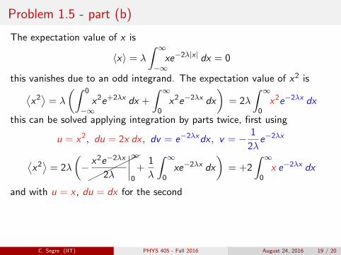
Problem 1.5 - part (b)
The expectation value of x is
〈x〉 = λ
∫ ∞−∞
xe−2λ|x | dx = 0
this vanishes due to an odd integrand. The expectation value of x2 is⟨x2⟩
= λ
(∫ 0
−∞x2e+2λx dx +
∫ ∞0
x2e−2λx dx
)= 2λ
∫ ∞0
x2e−2λx dx
this can be solved applying integration by parts twice, first using
u = x2, du = 2x dx , dv = e−2λxdx , v = − 1
2λe−2λx
⟨x2⟩
= 2λ
(−��
����x2e−2λx
2λ
∣∣∣∣∞0
+1
λ
∫ ∞0
xe−2λx dx
)= +2
∫ ∞0
x e−2λx dx
and with u = x , du = dx for the second
⟨x2⟩
= 2
(−��
���xe−2λx
2λ
∣∣∣∣∞0
+1
2λ
∫ ∞0
e−2λx dx
)= +
1
λ
∫ ∞0
e−2λx dx =1
2λ2
C. Segre (IIT) PHYS 405 - Fall 2016 August 24, 2016 19 / 20
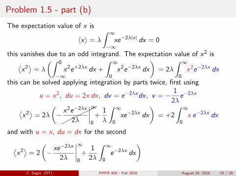
Problem 1.5 - part (b)
The expectation value of x is
〈x〉 = λ
∫ ∞−∞
xe−2λ|x | dx = 0
this vanishes due to an odd integrand. The expectation value of x2 is⟨x2⟩
= λ
(∫ 0
−∞x2e+2λx dx +
∫ ∞0
x2e−2λx dx
)= 2λ
∫ ∞0
x2e−2λx dx
this can be solved applying integration by parts twice, first using
u = x2, du = 2x dx , dv = e−2λxdx , v = − 1
2λe−2λx
⟨x2⟩
= 2λ
(−��
����x2e−2λx
2λ
∣∣∣∣∞0
+1
λ
∫ ∞0
xe−2λx dx
)= +2
∫ ∞0
x e−2λx dx
and with u = x , du = dx for the second
⟨x2⟩
= 2
(− xe−2λx
2λ
∣∣∣∣∞0
+1
2λ
∫ ∞0
e−2λx dx
)
= +1
λ
∫ ∞0
e−2λx dx =1
2λ2
C. Segre (IIT) PHYS 405 - Fall 2016 August 24, 2016 19 / 20

Problem 1.5 - part (b)
The expectation value of x is
〈x〉 = λ
∫ ∞−∞
xe−2λ|x | dx = 0
this vanishes due to an odd integrand. The expectation value of x2 is⟨x2⟩
= λ
(∫ 0
−∞x2e+2λx dx +
∫ ∞0
x2e−2λx dx
)= 2λ
∫ ∞0
x2e−2λx dx
this can be solved applying integration by parts twice, first using
u = x2, du = 2x dx , dv = e−2λxdx , v = − 1
2λe−2λx
⟨x2⟩
= 2λ
(−��
����x2e−2λx
2λ
∣∣∣∣∞0
+1
λ
∫ ∞0
xe−2λx dx
)= +2
∫ ∞0
x e−2λx dx
and with u = x , du = dx for the second
⟨x2⟩
= 2
(−��
���xe−2λx
2λ
∣∣∣∣∞0
+1
2λ
∫ ∞0
e−2λx dx
)
= +1
λ
∫ ∞0
e−2λx dx =1
2λ2
C. Segre (IIT) PHYS 405 - Fall 2016 August 24, 2016 19 / 20
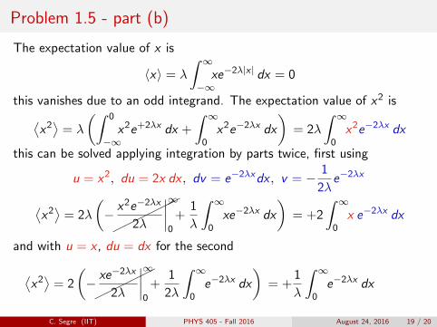
Problem 1.5 - part (b)
The expectation value of x is
〈x〉 = λ
∫ ∞−∞
xe−2λ|x | dx = 0
this vanishes due to an odd integrand. The expectation value of x2 is⟨x2⟩
= λ
(∫ 0
−∞x2e+2λx dx +
∫ ∞0
x2e−2λx dx
)= 2λ
∫ ∞0
x2e−2λx dx
this can be solved applying integration by parts twice, first using
u = x2, du = 2x dx , dv = e−2λxdx , v = − 1
2λe−2λx
⟨x2⟩
= 2λ
(−��
����x2e−2λx
2λ
∣∣∣∣∞0
+1
λ
∫ ∞0
xe−2λx dx
)= +2
∫ ∞0
x e−2λx dx
and with u = x , du = dx for the second
⟨x2⟩
= 2
(−��
���xe−2λx
2λ
∣∣∣∣∞0
+1
2λ
∫ ∞0
e−2λx dx
)= +
1
λ
∫ ∞0
e−2λx dx
=1
2λ2
C. Segre (IIT) PHYS 405 - Fall 2016 August 24, 2016 19 / 20
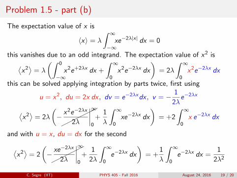
Problem 1.5 - part (b)
The expectation value of x is
〈x〉 = λ
∫ ∞−∞
xe−2λ|x | dx = 0
this vanishes due to an odd integrand. The expectation value of x2 is⟨x2⟩
= λ
(∫ 0
−∞x2e+2λx dx +
∫ ∞0
x2e−2λx dx
)= 2λ
∫ ∞0
x2e−2λx dx
this can be solved applying integration by parts twice, first using
u = x2, du = 2x dx , dv = e−2λxdx , v = − 1
2λe−2λx
⟨x2⟩
= 2λ
(−��
����x2e−2λx
2λ
∣∣∣∣∞0
+1
λ
∫ ∞0
xe−2λx dx
)= +2
∫ ∞0
x e−2λx dx
and with u = x , du = dx for the second
⟨x2⟩
= 2
(−��
���xe−2λx
2λ
∣∣∣∣∞0
+1
2λ
∫ ∞0
e−2λx dx
)= +
1
λ
∫ ∞0
e−2λx dx =1
2λ2
C. Segre (IIT) PHYS 405 - Fall 2016 August 24, 2016 19 / 20

Problem 1.5 - part (c)
The variance is now given by
σ2 =⟨x2⟩− 〈x〉2 =
1
2λ2− 0 =
1
2λ2
σ =1√2λ
λ
-2λ -σ 0 +σ +2λ
|Ψ|2
x
and the probability that the particle is outside the interval −σ < x < σ is
Pout = λ
∫ −σ−∞
e2λx dx + λ
∫ ∞σ
e−2λx dx = 2λ
∫ ∞σ
e−2λx dx
= 2λ
(−e−2λx
2λ
)∣∣∣∣∞σ
= e−2λσ
= e−2λ/√
2λ = e−√
2 = 0.2431
C. Segre (IIT) PHYS 405 - Fall 2016 August 24, 2016 20 / 20
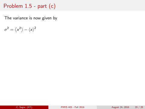
Problem 1.5 - part (c)
The variance is now given by
σ2 =⟨x2⟩− 〈x〉2
=1
2λ2− 0 =
1
2λ2
σ =1√2λ
λ
-2λ -σ 0 +σ +2λ
|Ψ|2
x
and the probability that the particle is outside the interval −σ < x < σ is
Pout = λ
∫ −σ−∞
e2λx dx + λ
∫ ∞σ
e−2λx dx = 2λ
∫ ∞σ
e−2λx dx
= 2λ
(−e−2λx
2λ
)∣∣∣∣∞σ
= e−2λσ
= e−2λ/√
2λ = e−√
2 = 0.2431
C. Segre (IIT) PHYS 405 - Fall 2016 August 24, 2016 20 / 20
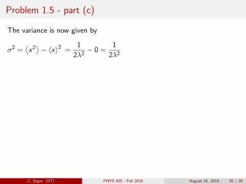
Problem 1.5 - part (c)
The variance is now given by
σ2 =⟨x2⟩− 〈x〉2 =
1
2λ2− 0 =
1
2λ2
σ =1√2λ
λ
-2λ -σ 0 +σ +2λ
|Ψ|2
x
and the probability that the particle is outside the interval −σ < x < σ is
Pout = λ
∫ −σ−∞
e2λx dx + λ
∫ ∞σ
e−2λx dx = 2λ
∫ ∞σ
e−2λx dx
= 2λ
(−e−2λx
2λ
)∣∣∣∣∞σ
= e−2λσ
= e−2λ/√
2λ = e−√
2 = 0.2431
C. Segre (IIT) PHYS 405 - Fall 2016 August 24, 2016 20 / 20
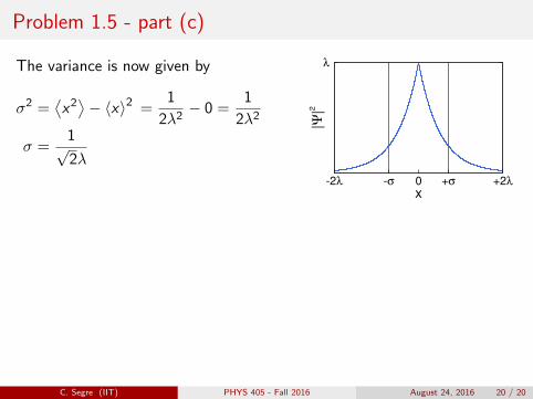
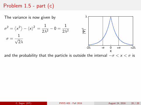
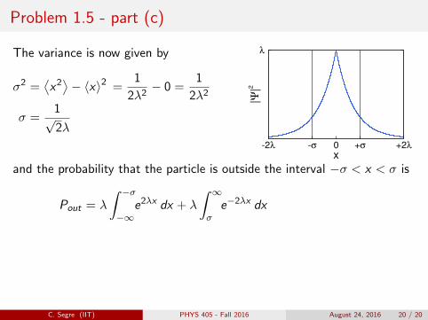
Problem 1.5 - part (c)
The variance is now given by
σ2 =⟨x2⟩− 〈x〉2 =
1
2λ2− 0 =
1
2λ2
σ =1√2λ
λ
-2λ -σ 0 +σ +2λ
|Ψ|2
x
and the probability that the particle is outside the interval −σ < x < σ is
Pout = λ
∫ −σ−∞
e2λx dx + λ
∫ ∞σ
e−2λx dx
= 2λ
∫ ∞σ
e−2λx dx
= 2λ
(−e−2λx
2λ
)∣∣∣∣∞σ
= e−2λσ
= e−2λ/√
2λ = e−√
2 = 0.2431
C. Segre (IIT) PHYS 405 - Fall 2016 August 24, 2016 20 / 20
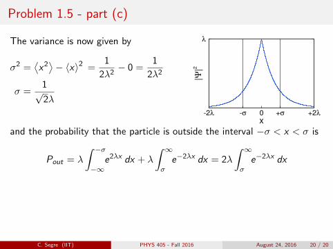
Problem 1.5 - part (c)
The variance is now given by
σ2 =⟨x2⟩− 〈x〉2 =
1
2λ2− 0 =
1
2λ2
σ =1√2λ
λ
-2λ -σ 0 +σ +2λ
|Ψ|2
x
and the probability that the particle is outside the interval −σ < x < σ is
Pout = λ
∫ −σ−∞
e2λx dx + λ
∫ ∞σ
e−2λx dx = 2λ
∫ ∞σ
e−2λx dx
= 2λ
(−e−2λx
2λ
)∣∣∣∣∞σ
= e−2λσ
= e−2λ/√
2λ = e−√
2 = 0.2431
C. Segre (IIT) PHYS 405 - Fall 2016 August 24, 2016 20 / 20
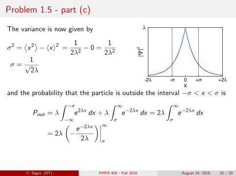
Problem 1.5 - part (c)
The variance is now given by
σ2 =⟨x2⟩− 〈x〉2 =
1
2λ2− 0 =
1
2λ2
σ =1√2λ
λ
-2λ -σ 0 +σ +2λ
|Ψ|2
x
and the probability that the particle is outside the interval −σ < x < σ is
Pout = λ
∫ −σ−∞
e2λx dx + λ
∫ ∞σ
e−2λx dx = 2λ
∫ ∞σ
e−2λx dx
= 2λ
(−e−2λx
2λ
)∣∣∣∣∞σ
= e−2λσ
= e−2λ/√
2λ = e−√
2 = 0.2431
C. Segre (IIT) PHYS 405 - Fall 2016 August 24, 2016 20 / 20
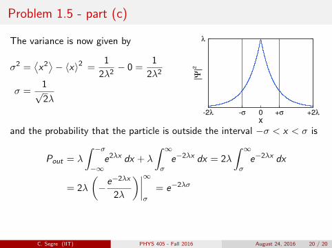
Problem 1.5 - part (c)
The variance is now given by
σ2 =⟨x2⟩− 〈x〉2 =
1
2λ2− 0 =
1
2λ2
σ =1√2λ
λ
-2λ -σ 0 +σ +2λ
|Ψ|2
x
and the probability that the particle is outside the interval −σ < x < σ is
Pout = λ
∫ −σ−∞
e2λx dx + λ
∫ ∞σ
e−2λx dx = 2λ
∫ ∞σ
e−2λx dx
= 2λ
(−e−2λx
2λ
)∣∣∣∣∞σ
= e−2λσ
= e−2λ/√
2λ = e−√
2 = 0.2431
C. Segre (IIT) PHYS 405 - Fall 2016 August 24, 2016 20 / 20
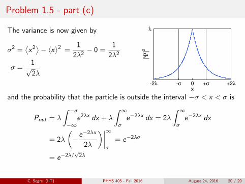
Problem 1.5 - part (c)
The variance is now given by
σ2 =⟨x2⟩− 〈x〉2 =
1
2λ2− 0 =
1
2λ2
σ =1√2λ
λ
-2λ -σ 0 +σ +2λ
|Ψ|2
x
and the probability that the particle is outside the interval −σ < x < σ is
Pout = λ
∫ −σ−∞
e2λx dx + λ
∫ ∞σ
e−2λx dx = 2λ
∫ ∞σ
e−2λx dx
= 2λ
(−e−2λx
2λ
)∣∣∣∣∞σ
= e−2λσ
= e−2λ/√
2λ
= e−√
2 = 0.2431
C. Segre (IIT) PHYS 405 - Fall 2016 August 24, 2016 20 / 20
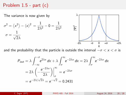
Problem 1.5 - part (c)
The variance is now given by
σ2 =⟨x2⟩− 〈x〉2 =
1
2λ2− 0 =
1
2λ2
σ =1√2λ
λ
-2λ -σ 0 +σ +2λ
|Ψ|2
x
and the probability that the particle is outside the interval −σ < x < σ is
Pout = λ
∫ −σ−∞
e2λx dx + λ
∫ ∞σ
e−2λx dx = 2λ
∫ ∞σ
e−2λx dx
= 2λ
(−e−2λx
2λ
)∣∣∣∣∞σ
= e−2λσ
= e−2λ/√
2λ = e−√
2 = 0.2431
C. Segre (IIT) PHYS 405 - Fall 2016 August 24, 2016 20 / 20


