Federal Reserve Bank of Dallas Globalization and Monetary Policy Institute
Working Paper No. 139 http://www.dallasfed.org/assets/documents/institute/wpapers/2013/0139.pdf
Trade Barriers and the Relative Price Tradables*
Michael Sposi
Federal Reserve Bank of Dallas
February 2013
Abstract In this paper I quantitatively address the role of trade barriers in explaining why prices of services relative to tradables are positively correlated with levels of development across countries. I argue that trade barriers play a crucial role in shaping the cross-country pattern of specialization across many heterogenous tradable goods. The pattern of specialization feeds into cross-country productivity differences in the tradables sector and is reflected in the relative price of services. I show that the existing pattern of specialization implies that the tradables-sector productivity gap between rich and poor countries is more than 80 percent larger than it would be under free trade. In turn, removing trade barriers would eliminate 64 percent of the disparity in the relative price of services between rich and poor countries, without systematically altering the cross-country pattern of the absolute price of tradables. JEL codes: F1, O4
* Michael Sposi, Research Department, Federal Reserve Bank of Dallas, 2200 N. Pearl Street, Dallas, TX 75201. 214-922-5881. [email protected]. I thank B. Ravikumar for his continual guidance and Raymond Riezman for his many suggestions. Special thanks also go to Mario Crucini and Hakan Yilmazkuday for sharing their micro-level estimates of distribution margins. This paper also benefited greatly from comments made by Elias Dinopoulos, Alex Monge-Naranjo, Sergio Rebelo, Ina Simonovska, Gustavo Ventura, Jing Zhang, and audiences at the Dallas Fed, St. Louis Fed, University of Iowa and the Fall 2012 Midwest Macroeconomics Meetings. Valerie Grossman provided excellent research assistance. All errors are my own. The views in this paper are those of the author and do not necessarily reflect the views of the Federal Reserve Bank of Dallas or the Federal Reserve System.

1 Introduction
In this paper I investigate the role that trade barriers play in explaining why prices of services
relative to tradables are positively correlated with levels of development across countries.
My main message is that trade barriers are crucial in shaping the cross-country pattern of
specialization across many heterogenous tradable goods. The pattern of specialization is
key in determining cross-country productivity differences in the tradables sector, and these
productivity differences are reflected in the relative price of services. I show that the existing
pattern of specialization implies that the tradables-sector productivity gap between rich and
poor countries is more than 80 percent larger than it would be if there were no barriers to
trade. In turn, removing trade barriers would eliminate 64 percent of the disparity in the
relative price of services between rich and poor countries. In particular, moving to free trade
does not systematically alter the cross-country pattern in the price of tradables, but it does
result in a large reduction in the gap in the price of services between rich and poor countries.
I construct aggregate prices for 103 countries for the year 2005 using detailed disaggregate
price data from the 2005 International Comparison Program, World Bank Development
Data Group (ICP from now on). I investigate country-specific PPPs at the retail level for
101 “Basic Headings” categories. I classify the Basic Heading categories into two groups:
goods and services. Broadly speaking, goods correspond to merchandise, while services are
intangible.
The ICP data are collected at the retail level which means that the observed prices
include a distribution margin. Thus, within “goods” I distinguish between retail goods and
tradable goods: retail goods are the products that result from combining tradable goods
with a distribution margin from the local dock (if the good is imported) or from the factory
gate (if the good is purchased domestically) to the final consumer. As a result, within each
country, the price of retail goods is different from the price of purely tradable goods. For
each country I construct two prices from Basic Headings data: one for services and one
for retail goods. The 2005 Benchmark study of the Penn World Tables, which is based on
ICP data, provides comparable prices across countries for a category called “Machinery and
equipment”. I take the price of Machinery and equipment to be my benchmark measurement
for the price of purely tradable goods for two reasons. First, Machinery and equipment are
highly traded and have a substantially smaller distribution margin than consumption goods
(Burstein, Neves, and Rebelo, 2004). Second, I prefer to use a parameter-free measurement
of the price of tradables as my benchmark. In section 4.2 I compare this proxy of the price of
tradables to parametric alternatives that rely on stripping away the distribution margin from
retail goods prices. By appealing to independent estimates of distribution margins in the
2
literature I show that the parametric constructions also lead to aggregate prices of tradables
that are uncorrelated with development.
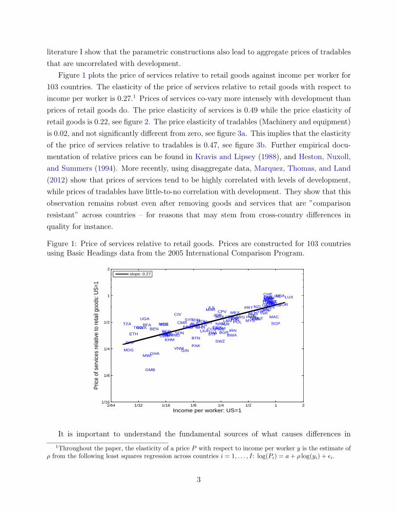
Figure 1 plots the price of services relative to retail goods against income per worker for
103 countries. The elasticity of the price of services relative to retail goods with respect to
income per worker is 0.27.1 Prices of services co-vary more intensely with development than
prices of retail goods do. The price elasticity of services is 0.49 while the price elasticity of
retail goods is 0.22, see figure 2. The price elasticity of tradables (Machinery and equipment)
is 0.02, and not significantly different from zero, see figure 3a. This implies that the elasticity
of the price of services relative to tradables is 0.47, see figure 3b. Further empirical docu-
mentation of relative prices can be found in Kravis and Lipsey (1988), and Heston, Nuxoll,
and Summers (1994). More recently, using disaggregate data, Marquez, Thomas, and Land
(2012) show that prices of services tend to be highly correlated with levels of development,
while prices of tradables have little-to-no correlation with development. They show that this
observation remains robust even after removing goods and services that are ”comparison
resistant” across countries – for reasons that may stem from cross-country differences in
quality for instance.
Figure 1: Price of services relative to retail goods. Prices are constructed for 103 countriesusing Basic Headings data from the 2005 International Comparison Program.
1/64 1/32 1/16 1/8 1/4 1/2 1 21/16
1/8
1/4
1/2
1
2
Income per worker: US=1
Pric
e of
ser
vice
s re
lativ
e to
reta
il go
ods:
US
=1
ALB
ARG
AUSAUTBEL
BENBFA
BGD BGRBOL
BRA
BTNBWA
CAF
CAN
CHE
CHL
CHN
CIV
CMR
COL
COM
CPV CYP
DNK
ECUEGY
ESP
ETH
FIN
FJI
FRAGBRGER
GHAGIN
GMB
GRCHKG
HUNIDN
IND
IRL
IRN
ISL
ISR
ITA
JORJPN
KENKHM
KORLBN
LKA
LUX
MAC
MAR
MDG
MDV
MEX
MLI
MLT
MNG
MOZ
MRT
MUS
MWI
MYSNAM
NLDNORNZL OMN
PAK
PANPERPHL
POL
PRT
PRYROMRWA
SAU
SDN
SEN SGP
STP
SWE
SWZ
SYR
TGOTHA
TTOTUNTURTZA
UGAURY
USA
VEN
VNM
ZAF
ZMB
slope: 0.27
It is important to understand the fundamental sources of what causes differences in
1Throughout the paper, the elasticity of a price P with respect to income per worker y is the estimate ofρ from the following least squares regression across countries i = 1, . . . , I: log(Pi) = a + ρ log(yi) + ϵi.
3

Figure 2: Prices of services and retail goods. Prices are constructed for 103 countries usingBasic Headings data from the 2005 International Comparison Program.
(a) Price of services.
1/64 1/32 1/16 1/8 1/4 1/2 1 21/16
1/8
1/4
1/2
1
2
Income per worker: US=1
Price
of
se
rvic
es:
US
=1
ALB
ARG
AUSAUTBEL
BENBFA
BGD
BGR
BOL
BRA
BTN
BWA
CAF
CAN
CHE
CHL
CHN
CIV
CMRCOL
COM
CPV
CYP
DNK
ECU
EGY
ESP
ETH
FIN
FJI
FRAGBRGER
GHA
GIN
GMB
GRC
HKG
HUN
IDN
IND
IRL
IRN
ISL
ISR
ITA
JOR
JPN
KEN
KHM
KOR
LBN
LKA
LUX
MACMAR
MDG
MDV
MEX
MLI
MLT
MNG
MOZ
MRT
MUS
MWI
MYS
NAM
NLD
NOR
NZL
OMN
PAK
PANPER
PHL
POL
PRT
PRY
ROM
RWA
SAU
SDN
SEN
SGP
STP
SWE
SWZSYRTGO
THA
TTO
TUN
TUR
TZA
UGA
URY
USA
VEN
VNM
ZAF
ZMB
slope: 0.49
(b) Price of retail goods.
1/64 1/32 1/16 1/8 1/4 1/2 1 21/16
1/8
1/4
1/2
1
2
Income per worker: US=1
Price
of
reta
il g
oo
ds:
US
=1
ALB
ARG
AUSAUTBEL
BENBFA
BGD
BGR
BOL
BRA
BTN
BWA
CAF
CANCHE
CHL
CHNCIVCMR
COLCOM
CPV
CYP
DNK
ECU
EGY
ESP
ETH
FIN
FJI
FRAGBRGER
GHA
GINGMB
GRC
HKGHUN
IDNIND
IRL
IRN
ISL
ISR
ITA
JOR
JPN
KEN
KHM
KOR
LBN
LKA
LUX
MAC
MAR
MDG
MDV MEXMLI
MLT
MNG
MOZMRT MUSMWIMYS
NAM
NLD
NOR
NZL
OMN
PAK
PANPER
PHL
POL
PRT
PRY
ROM
RWA
SAUSDNSEN
SGP
STP
SWE
SWZ
SYR
TGOTHA
TTO
TUN
TUR
TZA
UGA
URY
USA
VEN
VNM
ZAFZMB
slope: 0.22
Figure 3: Price of tradables. I use the category “Machinery and equipment” from the 2005ICP as a stand in for tradables.
(a) Price of tradables.
1/64 1/32 1/16 1/8 1/4 1/2 1 21/16
1/8
1/4
1/2
1
2
Income per worker: US=1
Price
of
tra
da
ble
s:
US
=1
ALB ARGAUSAUTBEL
BEN
BFA BGD BGR
BOL BRABTN
BWA
CAF CANCHE
CHLCHNCIV
CMR COL
COM CPVCYP DNK
ECUEGY
ESPETHFIN
FJIFRAGBRGER
GHAGIN
GMB
GRC
HKGHUNIDN
IND
IRL
IRN
ISLISRITA
JOR
JPN
KEN
KHM
KOR
LBN
LKALUX
MAC
MAR
MDG
MDV
MEXMLI MLTMNGMOZMRT MUS
MWI
MYSNAM
NLD
NORNZL
OMN
PAK PAN
PERPHL
POLPRTPRY
ROMRWA
SAU
SDNSENSGP
STP
SWESWZ
SYRTGO
THA TTO
TUN
TUR
TZA
UGAURY
USA
VEN
VNM ZAF
ZMB
slope: 0.02
(b) Price of services relative to tradables.
1/64 1/32 1/16 1/8 1/4 1/2 1 21/16
1/8
1/4
1/2
1
2
Income per worker: US=1
Price
of
se
rvic
es r
ela
tive
to
tra
da
ble
s:
US
=1
ALB
ARG
AUSAUTBEL
BEN
BFA
BGD
BGR
BOL
BRA
BTN
BWA
CAF
CAN
CHE
CHL
CHN
CIV
CMRCOL
COM
CPV
CYP
DNK
ECU
EGY
ESP
ETH
FIN
FJI
FRAGBR
GER
GHA
GIN
GMB
GRCHKG
HUN
IDNIND
IRL
IRN
ISL
ISR
ITA
JOR
JPN
KEN
KHM
KORLBN
LKA
LUX
MAC
MAR
MDG
MDV MEX
MLI
MLT
MNG
MOZ
MRT
MUS
MWI
MYSNAM
NLD NOR
NZL
OMN
PAK
PAN
PER
PHL
POL
PRT
PRY
ROM
RWA
SAU
SDN
SEN
SGP
STP
SWE
SWZ
SYRTGO THA
TTOTUN
TUR
TZA
UGA
URY
USA
VEN
VNM
ZAF
ZMB
slope: 0.47
4

relative prices across countries for at least two reasons. First, relative prices lie at the heart
of understanding real exchange rates (see for instance Burstein, Eichenbaum, and Rebelo,
2005). Second, relative prices play a crucial role in understanding income differences across
countries (Restuccia and Urrutia, 2001; Eaton and Kortum, 2002; Hsieh and Klenow, 2007).
An early explanation as to why relative prices co-vary positively with development is due
to Balassa (1964) and Samuelson (1964), the celebrated Balassa-Samuelson hypothesis. The
theory implies that larger cross-country productivity differences in tradables than in nontrad-
ables result in larger cross-country differences in the price of nontradables than in the price
of tradables. The intuition is as follows. Free trade and no arbitrage force the price of trad-
ables to be equal across countries. Tradables-sector productivity is higher in rich countries
than in poor countries resulting in higher wages in rich countries, and therefore, higher pro-
duction costs. Mobility of homogeneous labor across sectors leads to higher production costs
in rich countries’ nontradables sector. This, coupled with small cross-country productivity
differences in nontradables, results in a higher price of nontradables in rich countries than
in poor countries. In particular, in each country, the relative price of nontradables is equal
to the inverse of its relative productivity. Herrendorf and Valentinyi (2012) argue that the
Balassa-Samuelson effect holds in a large cross section of countries: measured cross-country
productivity differences are larger in tradables than in nontradables.
Bergin, Glick, and Taylor (2006) argue that the cross-country productivity gap is higher
in tradables than in nontradables because more productive firms drive out less productive
firms, and more productive firms tend to produce tradable goods. Buera, Kaboski, and Shin
(2011) argue that financial frictions result in a misallocation of productive resources across
sectors resulting in larger cross-country productivity differences in goods than in services.
I argue that existing trade barriers result in a misallocation of the production of tradable
goods and thus magnify the cross-country productivity gap in tradables. To this end, my
paper encompasses the Balassa-Samuelson argument by providing a mechanism for which
productivity differences in the tradables sector endogenously arise. However, my paper does
not rely on the free trade assumption. In fact, I interact my model with data on bilateral
trade in order to measure trade barriers, and the model in turn produces relative prices that
are inline with the data in spite of, and more importantly as a result of, the fact that the
calibrated trade barriers are nontrivial.2
A related strand of literature focusses exclusively on cross-country variation in the prices
2Waugh (2010) shows that that, in order to be simultaneously consistent with aggregate prices of tradablegoods and the pattern of bilateral trade within a gravity framework, poor countries must face systematicallylarger barriers to export than rich countries. He then shows the implications that this particular pattern oftrade barriers has for aggregate TFP and cross-country income differences.
5

of retail goods. Simonovska (2010) focuses on the positive correlation between prices of
tradables (at the retail level) and levels of development. Using evidence from a particular
apparel exporter, she shows that price discrimination across destinations is quantitatively
important. Giri (2012) shows that incorporating distribution margins into a Ricardian model
of trade with trade barriers can help explain the cross-sectional pattern of prices of retail
goods across countries. Crucini and Yilmazkuday (2009) study retail price dispersion across
international cities. They develop a two-sector, multi-city, general equilibrium model with
a large number of goods and good-specific distribution margins. They use their model to
estimate distribution margins for each good and quantify the importance of both trade costs
and distribution costs on deviations from the law of one price.
I construct a multi-country model of trade with a continuum tradable goods. Each
country has technologies for producing each tradable good, a composite good, nontradable
services, and retail goods. Production of all tradables and services requires capital, labor,
and intermediate inputs. Intermediate inputs consist of services and the composite good.
Each country’s level of efficiency for each tradable good is a random draw from a Frechet
distribution. Countries differ in their average efficiency across tradable goods and also face
asymmetric bilateral trade barriers. Countries also differ in their services productivity. Each
country purchases each tradable good from its least cost supplier, and all tradable goods
are aggregated to form the composite good. Retail goods are constructed by applying a
distribution margin, in the form of services, to the composite good. Finally, retail goods and
services are used for final consumption. In equilibrium, each country produces only a subset
of the tradable goods. Therefore, measured productivity in the tradables sector depends on
the subset of goods produced, and the subset depends on the pattern of trade barriers.
I apply the model to a set of 103 countries for the year 2005. I quantitatively discipline
the parameters of the model to be consistent with the observed pattern of bilateral trade
and cross-country relative levels of development. Novel to the model is the feature that
productivity in tradables depends crucially on the trade barriers. The calibration implies
that poor countries face larger trade barriers than rich countries do. The resulting pattern
of specialization leads to cross-country productivity differences in tradables that are twice
as large as cross-country productivity differences in services.
The calibrated model reproduces the positive correlation between the prices of services
and levels of development: the price elasticity of services (with respect to income per worker)
is 0.59 in the model and is 0.49 in the data. The model replicates the distribution of the
price of tradables almost perfectly: the price elasticity of tradables is 0.01 in the model and
is 0.02 in the data. In the model, the price of retail goods is a geometric average of the
price of services and the price of tradables, with the weight on the price of services equal to
6
the distribution margin. Thus, the model slightly over-states the difference in the price of
retail goods between rich and poor countries: the price elasticity of retail goods is 0.30 in
the model and is 0.22 in the data.
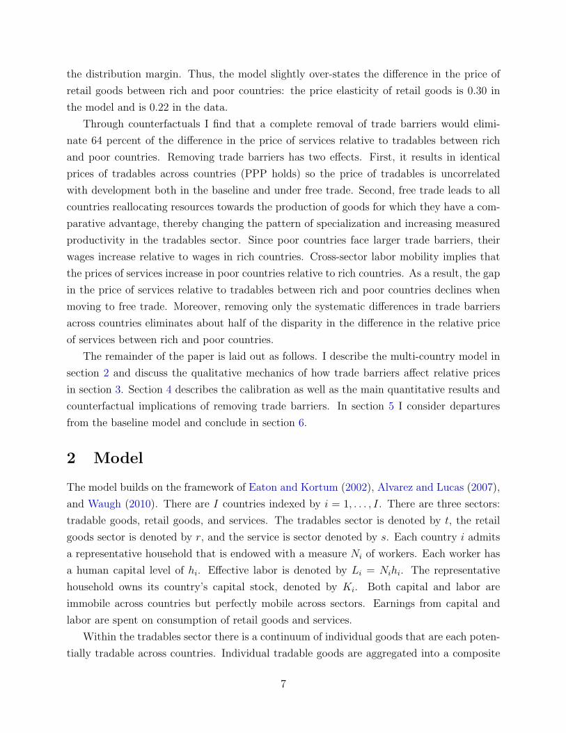
Through counterfactuals I find that a complete removal of trade barriers would elimi-
nate 64 percent of the difference in the price of services relative to tradables between rich
and poor countries. Removing trade barriers has two effects. First, it results in identical
prices of tradables across countries (PPP holds) so the price of tradables is uncorrelated
with development both in the baseline and under free trade. Second, free trade leads to all
countries reallocating resources towards the production of goods for which they have a com-
parative advantage, thereby changing the pattern of specialization and increasing measured
productivity in the tradables sector. Since poor countries face larger trade barriers, their
wages increase relative to wages in rich countries. Cross-sector labor mobility implies that
the prices of services increase in poor countries relative to rich countries. As a result, the gap
in the price of services relative to tradables between rich and poor countries declines when
moving to free trade. Moreover, removing only the systematic differences in trade barriers
across countries eliminates about half of the disparity in the difference in the relative price
of services between rich and poor countries.
The remainder of the paper is laid out as follows. I describe the multi-country model in
section 2 and discuss the qualitative mechanics of how trade barriers affect relative prices
in section 3. Section 4 describes the calibration as well as the main quantitative results and
counterfactual implications of removing trade barriers. In section 5 I consider departures
from the baseline model and conclude in section 6.
2 Model
The model builds on the framework of Eaton and Kortum (2002), Alvarez and Lucas (2007),
and Waugh (2010). There are I countries indexed by i = 1, . . . , I. There are three sectors:
tradable goods, retail goods, and services. The tradables sector is denoted by t, the retail
goods sector is denoted by r, and the service is sector denoted by s. Each country i admits
a representative household that is endowed with a measure Ni of workers. Each worker has
a human capital level of hi. Effective labor is denoted by Li = Nihi. The representative
household owns its country’s capital stock, denoted by Ki. Both capital and labor are
immobile across countries but perfectly mobile across sectors. Earnings from capital and
labor are spent on consumption of retail goods and services.
Within the tradables sector there is a continuum of individual goods that are each poten-
tially tradable across countries. Individual tradable goods are aggregated into a composite
7
good. Each individual tradable good is produced using capital, labor, the composite good,
and services. Services are produced using capital, labor, the composite good, and services as
well. Services are combined with the composite good to construct retail goods. Neither retail
goods nor services are tradable. From now on, where it is understood, country subscripts
are omitted.
I choose world GDP to be the numeraire of the economy, i.e.,∑
i wiLi + riKi = 1, where
wi and ri denote the rental rates for labor and capital respectively in country i. Hence, all
units are expressed in terms of world output.
2.1 Technologies
There is a continuum of individual tradable goods indexed by x ∈ [0, 1], and each individual
good is potentially tradable.
Composite intermediate good All individual tradable goods along the continuum
are aggregated into a composite intermediate good T according to
T =
(∫qt(x)
η−1η dx
) ηη−1
.
where qt(x) denotes the quantity of good x.
Individual tradable goods Each country has access to technologies for producing
each individual tradable good as follows
ti(x) = zi(x)−θ(Kti(x)αLti(x)1−α
)νt(Sti(x)σtTti(x)1−σt
)1−νt.
For each factor used in production, the subscript denotes the sector that uses the factor, and
the argument in the parentheses denotes the index of the good along the continuum. For
example, Kti(x), Lti(x), Sti(x), and Tti(x) respectively denote the amounts of capital, labor,
services, and composite good that country i uses to produce tradable good x. The parameter
νt ∈ [0, 1] determines the share of value added in gross production, σt ∈ [0, 1] determines the
share if services in intermediate inputs, while α ∈ [0, 1] determines capital’s share in value
added.
As in Alvarez and Lucas (2007), zi(x) represents country i’s cost of producing good x,
which is modeled as an independent random draw from an exponential distribution with
parameter λi > 0 in country i. This implies that zi(x)−θ, country i’s level of efficiency in
producing good x, has a Frechet distribution. The expected value of zi(x)−θ is λθi , so average
8

efficiency across the continuum of goods is λθi .
3 If λi > λj, then on average, country i is
more efficient than country j. The parameter θ > 0 governs the coefficient of variation in
efficiency across the continuum. A larger θ implies more variation in efficiency levels, and
hence, more room more specialization.
Since the index of the good x is irrelevant, from now on I follow Alvarez and Lucas (2007)
and identify each individual good x by its vector of cost draws: z = (z1(x), z2(x), . . . zI(x)).
I denote country i’s density for cost draws by φi(z).
Services Services are nontradable and are produced using capital and labor in addition
to two intermediate inputs: services and the composite good.
Si = Asi
(Kα
siL1−αsi
)νs(Sσs
si T 1−σssi
)1−νs.
The term Asi denotes country i’s productivity in the services sector.
Retail goods Retail goods are constructed by combining the composite good together
with domestic services.
Ri = Sσrri T 1−σr
ri .
This technology makes explicit the idea that a domestic service margin is applied to trad-
able goods (the composite good) after trade has taken place. The parameter σr ∈ [0, 1]
corresponds to the distribution margin.
2.2 Preferences
The representative household derives utility from consuming retail goods and services as
follows:
Ci = Cσcsi (Cri − Nicr)
1−σc .
The terms Cs and Cr denote aggregate consumption of services and retail goods respectively.
The term cr denotes a subsistence level (per worker) for consumption of retail goods and is
constant across countries.
2.3 International trade
Country i purchases each individual tradable good from its least cost supplier. The purchase
price depends on the unit cost of the producer, as well as trade barriers.
3In equilibrium, each country produces only a subset of these goods and imports the rest. Therefore,average measured productivity is endogenous because it depends on the set of goods produced.
9

Barriers to trade are denoted by τij, where τij > 1 is the amount of goods that country
j must export in order for one unit to arrive in country i. As a normalization I assume that
there are no barriers to ship goods domestically; that is, τii = 1 for all i. I also assume that
the triangle inequality holds: τijτjl ≥ τil.
2.4 Equilibrium
I focus on a competitive equilibrium. Informally, a competitive equilibrium is a set of prices
and allocations that satisfy the following conditions: 1) The representative household max-
imizes utility, taking prices as given 2) firms maximize profits, taking prices as given, 3)
domestic goods and factor markets clear and 4) trade is balanced in each country. In the
remainder of this section I describe each condition from country i’s point of view.
2.4.1 Household optimization
At the beginning of the time period, the capital stock is rented to domestic firms in each
sector at the competitive rental rate ri and labor is supplied domestically at the wage rate
wi. At the end of the period, factor income is spent on consumption of services and retail
goods which have respective prices Psi and Pri. Therefore the representative household faces
the following budget constraint.
PsiCsi + PriCri = wiLi + riKi.
Utility maximization implies that the representative household optimally allocates ex-
penditures as follows:
PsiCsi = σc(wiLi + riKi − PriNicr)
PriCri = (1 − σc)(wiLi + riKi − PriNicr) + PriNicr.
I restrict the parameter cr such that the representative household in each country has enough
income to cover the subsistence requirement, i.e., wiLi + riKi > PriNicr for all i.
I define an optimal price for discretionary consumption, Pci, such that: PciCi = PsiCsi +
Pri(Cri − Nicr). I show in appendix C that
Pci = BcPσcsi P 1−σc
ri , (1)
where Bc = (σc)−σc (1 − σc)
σc−1.
10

2.4.2 Firm optimization
Denote the price for an individual tradable good z that was produced in country j and
purchased by country i by ptij(z). Then, ptij(z) = ptjj(z)τij, where ptjj(z) is the marginal
cost of producing good z in country j. Since each country purchases each individual good
from its least cost supplier, the actual price in country i of good z is pti(z) = minj=1,...,I
[ptjj(z)τij].
The price of the composite good is
Pti =
(∫pti(z)1−ηφ(z)dz
) 11−η
,
where φ(z) is the joint density of cost draws across countries.
I explain how to derive the prices for each country in appendix C. Given the assumption
on the country-specific densities, φi, the model implies that
Pti = γBtuti(λi
πii
)θ, (2)
where uti =(rαi w1−α
i
)νt(P σt
si P 1−σtti
)1−νtis the unit cost for a factor bundle faced by pro-
ducers of tradables in country i. The term Bt = (ανt)−ανt((1 − α)νt)
(α−1)νt(σtνt)−σtνt((1 −
σt)νt)(σt−1)νt is constant across countries. Finally, the term γ = Γ (1 + θ(1 − η))
11−η is also
constant across countries, where Γ(·) is the Gamma function. I restrict parameters such that
γ > 0. Note that the price in country i is the unit cost of inputs in country i, divided by
country i’s average productivity, multiplied by technological parameters that are constant
across countries.4
The price of services is simply the unit cost of inputs, divided by productivity, scaled by
technological parameters:
Psi = Bsusi
Asi
.
The term usi =(rαi w1−α
i
)νs(P σs
si P 1−σsti
)1−νsis the cost of a factor bundle faced by produc-
ers of services in country i and Bs = (ανs)−ανs((1−α)νs)
(α−1)νs(σsνs)−σsνs((1−σs)νs)
(σs−1)νs
is constant across countries.
Finally, producers of retail goods in country i apply a distribution margin to the com-
posite good (the basket of tradables) by using domestic services. The result is that the price
of retail goods takes the following form.
Pri = BrPσrsi P 1−σr
ti ,
where Br = (σr)−σr(1 − σr)
σr−1 and σr is the distribution margin.
4Average productivity in tradables is (λi/πii)θ. This differs from average efficiency across the entirecontinuum of goods λθ
i since, in equilibrium, country i specializes in a subset of goods for which it iscomparatively “good” at producing. The measure of such goods is captured by πii.
11
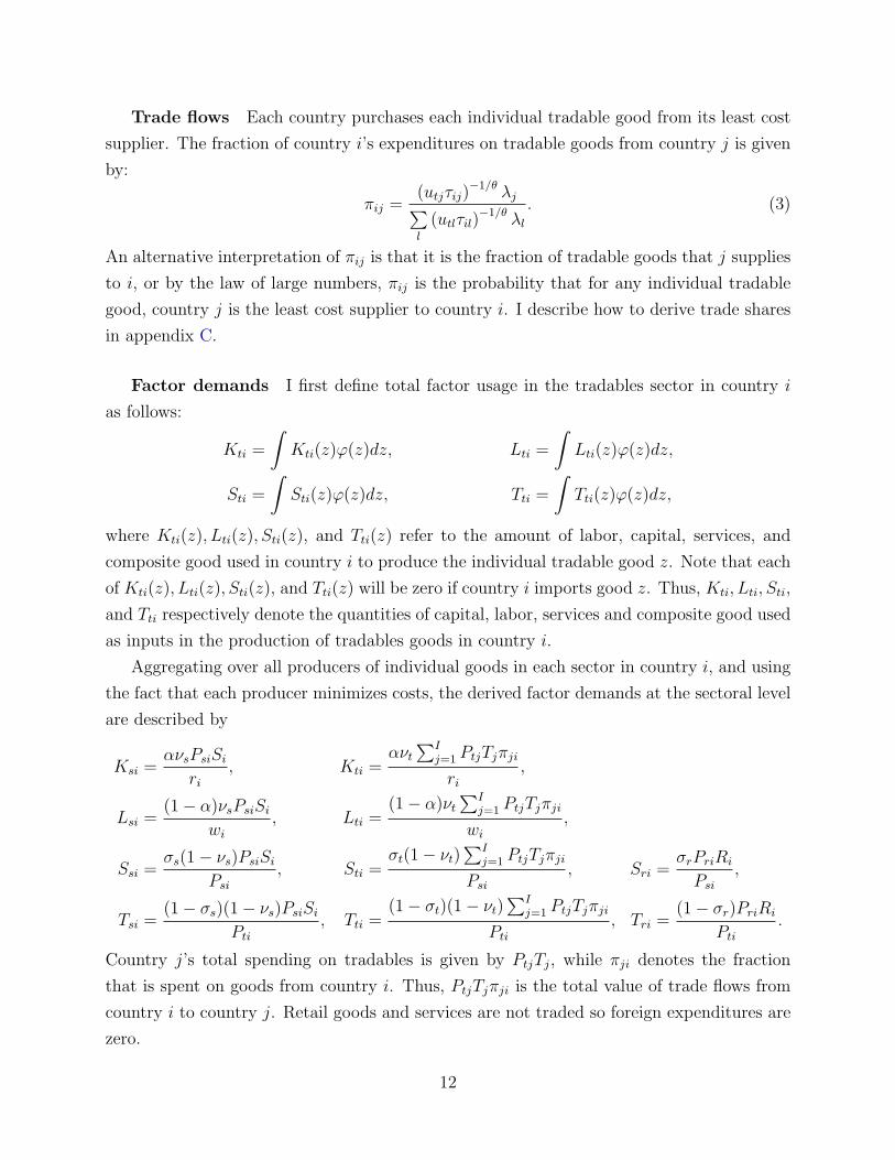
Trade flows Each country purchases each individual tradable good from its least cost
supplier. The fraction of country i’s expenditures on tradable goods from country j is given
by:
πij =(utjτij)
−1/θ λj∑l
(utlτil)−1/θ λl
. (3)
An alternative interpretation of πij is that it is the fraction of tradable goods that j supplies
to i, or by the law of large numbers, πij is the probability that for any individual tradable
good, country j is the least cost supplier to country i. I describe how to derive trade shares
in appendix C.
Factor demands I first define total factor usage in the tradables sector in country i
as follows:
Kti =
∫Kti(z)φ(z)dz, Lti =
∫Lti(z)φ(z)dz,
Sti =
∫Sti(z)φ(z)dz, Tti =
∫Tti(z)φ(z)dz,
where Kti(z), Lti(z), Sti(z), and Tti(z) refer to the amount of labor, capital, services, and
composite good used in country i to produce the individual tradable good z. Note that each
of Kti(z), Lti(z), Sti(z), and Tti(z) will be zero if country i imports good z. Thus, Kti, Lti, Sti,
and Tti respectively denote the quantities of capital, labor, services and composite good used
as inputs in the production of tradables goods in country i.
Aggregating over all producers of individual goods in each sector in country i, and using
the fact that each producer minimizes costs, the derived factor demands at the sectoral level
are described by
Ksi =ανsPsiSi
ri
, Kti =ανt
∑Ij=1 PtjTjπji
ri
,
Lsi =(1 − α)νsPsiSi
wi
, Lti =(1 − α)νt
∑Ij=1 PtjTjπji
wi
,
Ssi =σs(1 − νs)PsiSi
Psi
, Sti =σt(1 − νt)
∑Ij=1 PtjTjπji
Psi
, Sri =σrPriRi
Psi
,
Tsi =(1 − σs)(1 − νs)PsiSi
Pti
, Tti =(1 − σt)(1 − νt)
∑Ij=1 PtjTjπji
Pti
, Tri =(1 − σr)PriRi
Pti
.
Country j’s total spending on tradables is given by PtjTj, while πji denotes the fraction
that is spent on goods from country i. Thus, PtjTjπji is the total value of trade flows from
country i to country j. Retail goods and services are not traded so foreign expenditures are
zero.
12

2.4.3 Market clearing
The market clearing conditions for the raw factors of production (capital and labor) are:
Ksi + Kti = Ki and Lsi + Lti = Li.
The left-hand side of each of the previous equations is simply the factor usage by each sector,
while the right-hand side is the factor availability.
The remaining country-specific resource constraints require that produced goods be equal
to their uses.
Sri + Ssi + Sti + Csi = Si,
Tri + Tsi + Tti = Ti,
Cri = Ri
That is, the use of services as an intermediate in production plus final consumption of services
must equal the amount of services available. Similar for tradables and retail goods.
2.4.4 Trade balance
To close the model I impose balanced trade country by country.
PtiTi
∑j =i
πij =∑j =i
PtjTjπji,
where the left-hand side denotes country i’s imports, and the right-hand side denotes country
i’s exports.
This completes the description of a competitive equilibrium in the model. Next I discuss
some important equilibrium implications of the theoretical model.
3 Qualitative implications for relative prices
I first discuss how relative prices are determined qualitatively and expose how the trade
mechanism affects relative prices. Recall that the price of retail goods is Pri = BrPσrsi P 1−σr
ti .
Therefore, the price of services relative to retail goods is a simple transformation of the price
of services relative to tradables: Psi
Pri=(
1Br
)(Psi
Pti
)1−σr
. Since the term Br is constant across
countries, Ps/Pr is isomorphic to Ps/Pt as long as σr < 1. Thus, understanding the price of
services relative to tradables is equivalent to understanding the price of services relative to
retail goods with one key distinction; the price of services relative to retail goods includes the
term 1− σr in the exponent. This term accounts for the distribution margin in retail goods.
13

In particular, if there are no services required in distribute tradable goods to consumers, i.e.,
σr = 0 then this exponent is unity and the two relative prices are identical up to a constant
of proportionality. A larger σr implies a larger share of services in the production of retail
goods, thus the absolute price of retail goods will more closely resemble the absolute price
of services.
I show in appendix C that the price of services relative to tradables is
Psi
Pti
= Ψ ×
[(λi/πii)
θ] νs
νt
Asi
1
1−σs(1−νs)+σt(1−νt)νs/νt
, (4)
where Ψ is a collection of terms that are constant across countries. Thus, the price of services
relative to retail goods is
Psi
Pri
=
(Ψ1−σr
Br
)[(λi/πii)
θ] νs
νt
Asi
1−σr
1−σs(1−νs)+σt(1−νt)νs/νt
. (5)
In order to interpret equations (4) and (5), note that they boil down to country i’s pro-
ductivity in tradables divided by country i’s productivity in services (the second term in
each expression). To see this recall that country i’s average efficiency across all individual
tradable goods is λθi . However, country i specializes in only a subset of the tradable goods.
Therefore, its average measured productivity is its average efficiency, λθi , corrected by the
share of goods that it actually produces, i.e., its home trade share, πii. The numerator is thus
average measured productivity in tradables: (λi/πii)θ. In the denominator is the productiv-
ity in services Asi. The remaining terms are common across countries and do not contribute
to the cross-country variation. Thus, the model produces the classic Balassa-Samuelson ef-
fect endogenously: the price of nontradables (services), relative to tradables, is equal to the
measured productivity in tradables, relative to the measured productivity in nontradables
(services), corrected by the relevant input-output coefficients. The terms in the exponent
adjust for the input-output structure since there is feed through across sectors: The price of
services enters the price of tradables, and the price of tradables enters the price of services,
since they are both used as intermediate inputs in production.
Novel to the model is that the average productivity in tradables depends on the endoge-
nous term πii, country i’s home trade share. The home trade share in country i reveals the
set of goods that country i specializes in producing. The more specialized a country is, the
smaller its home trade share is, and the higher its measured productivity in tradables will be.
The degree of specialization depends on average efficiency, as well as the pattern of bilateral
trade barriers.
14
4 Quantification
In this section I discuss the methodology for calibrating the model parameters. Then I
discuss the implications of the calibrated model for explaining the distribution of prices across
countries and assess the importance of trade barriers in generating the observed pattern of
prices.
4.1 Data and calibration
I calibrate the model using data for a set of 103 countries for the year 2005 (see table D.2
in appendix D for the complete list of countries). This set includes both developed and
developing countries and accounts for about 90 percent of the world GDP as computed from
version 6.3 of the Penn World Tables (see Heston, Summers, and Aten, 2009, PWT63).
4.1.1 Data
With respect to the trade and production data used, the tradables sector corresponds to
four-digit ISIC revision 2 categories 15⋆⋆–37⋆⋆. Trade data is reported at the four-digit SITC
revision 2 level. I use a correspondence between production data (ISIC) and trade data
(SITC) created by Affendy, Sim Yee, and Satoru (2010). The source for trade data is UN
Comtrade, and I obtain production data from two sources: INDSTAT 4, 2010 (a databases
maintained by UNIDO), and the World Bank’s World Bank Development Indicators (for
countries where data is not available through INDSTAT). The service sector accounts for
the remainder of GDP that is not accounted for by value added in tradables. In the model
there is a sector called retail goods. In terms of classification, I do not distinguish retail goods
from tradables and there is no additional value added at the retail level. The interpretation
is that retail goods are simply the tradable goods made available to final consumers by using
domestic distribution services; some portion of the tradable goods are imported, and the
remaining portion is purchased domestically.5
Construction of prices using ICP data I construct prices for services and retail
goods using detailed Basic Headings data from the 2005 International Comparison Program,
World Bank Development Data Group. The data I use is at the retail level for which there is
no one-to-one link with ISIC categories, so I take a stand on which categories are closest to
5An example is a computer. Think of each component of a computer (processor, memory, disk, keypad,etc.) as an individual tradable good. Each country purchases each component from their least cost supplier.Once each component is purchased (some maybe imported, some purchased domestically) they are bundledinto a composite good (a computer). Then the computer is sold to consumers by the domestic service sector(retail).
15

goods, and which are closest to services. There are 129 categories at the Basic Heading level,
53 of which I classify as retail goods, 48 as services, and the remaining 28 are unclassified (for
example, the category “Change in inventories and valuables” is left unclassified) see table
D.1 in appendix A for the complete list. The exact methodology I use to aggregate the Basic
Headings prices into sectoral aggregate prices is in explained in appendix A.
4.1.2 Common parameters
I begin by describing the parameters which are common across countries and given in table 1.
Following Alvarez and Lucas (2007), I set η equal to 2. This parameter is not quantitatively
important for the question addressed in this paper, however, it must satisfy 1+θ(1−η) > 0.
Capital’s share α is set at 1/3 as in Gollin (2002). This parameter is set so that labor’s
share in GDP is 2/3.
The parameters νs and νt, respectively, control the value added in services and tradable
goods production. I compute both parameters by taking the average of the ratio of value
added output to total output. For tradable goods I employ the manufacturing data from
the INDSTAT 4, 2010 database, and for services I employ input-output tables for OECD
countries.
The parameter σr corresponds to the distribution margin for retail goods.6 Berger, Faust,
Rogers, and Steverson (2012) argue that distribution margins in the US are on average be-
tween 0.50 and 0.70. Crucini and Yilmazkuday (2009) use micro data to construct estimates
of distribution margins across a large number of retail items and cities. For a subset of their
items that most closely correspond to my definition of retail goods, the median estimate
of distribution margins is 0.42. They also state that the aggregate distribution margin, as
measured from U.S. National Income and Product Accounts is 0.5, the same value that is
used in Burstein, Neves, and Rebelo (2003). Since I aggregate all goods into one sector in
my model, I set σr at 0.50, in line with the above evidence. At the end of the paper I check
the sensitivity of the model’s predictions over a range of values for the distribution margin.
The parameters σs and σt control the share of services (relative to tradables) as an input
in intermediate uses. In particular, 1 − σt corresponds to the share of manufactures in
total intermediate spending by producers of tradables. Using input-output tables for OECD
countries I compute σt = 0.17. Finally, σs corresponds to the share of spending on services
(including local distribution) in total intermediate spending by producers of services. I
calculate σs = 0.70 from input-output tables for OECD countries.
6Specifically, distribution includes retail and wholesale trade, and local transport and storage, markups,and value-added taxes.
16

Next I discuss the calibration of preference parameters: σc and cr. σc is the share of
services in the representative household’s discretionary expenditures, while cr is the per-
worker subsistence level of retail goods consumption.7 In my sample of 103 countries, the
richest countries spend about 60 percent of their income on services. Since subsistence
plays no role when income is high, I set σs = 0.60. The poorest countries in my sample
spend about 20 percent of their total income on services. Thus, I set the value cr such
that the poorest countries spend 20 percent of their income on services. I introduce non-
homothetic preferences to allow for the possibility that differences in relative prices are driven
by differences in relative demand. However, it turns out that demand-side forces contribute
next to nothing to the distribution of relative prices. If instead I set cr = 0 then all countries
spend 60 percent of their income on services, while all of the implications for prices are
essentially unaltered.
The parameter θ controls the dispersion in efficiency levels. I follow Alvarez and Lucas
(2007) and set this parameter at 0.15. This value lies in the middle of the estimates in Eaton
and Kortum (2002). My results hold up to other values including θ = 0.24, the preferred
estimate in Simonovska and Waugh (2010).
Table 1: Common parameters
Parameter Description Valueα K’s share in GDP 0.33νt K and L’s share in production of tradables 0.31νs K and L’s share in production of services 0.56σr service’s share in retail goods production (distribution margin) 0.50σs service’s share in intermediate component of services production 0.70σt service’s share in intermediate component of tradables production 0.17σc share of services in final discretionary expenditures 0.60cr subsistence level for consumption of retail goods per worker 0.08θ variation in efficiency levels 0.15η elasticity of substitution in aggregator 2
Note: The subsistence level cr implies that countries in the bottom decile of the income dis-tribution allocate 20 percent of their total consumption expenditures to services.
4.1.3 Country-specific parameters
I take the labor force N from PWT63. To construct measures of human capital h, I follow
Hall and Jones (1999) and Caselli (2005) by converting data on years of schooling from
7Discretionary expenditures refer to the representative household’s expenditures in excess of spending onsubsistence.
17
Barro and Lee (2010) into measures of human capital using Mincer returns. Effective labor
is then L = Nh, see appendix A for details. I construct capital stocks Ki using the perpetual
inventory method using investment data from PWT63, see appendix A for details.
The remaining parameters include the bilateral trade barriers τij, the average efficiency
parameters in the tradable sector, λi, and the productivity levels in the service sector, Asi.
My strategy is to choose these parameters to be consistent with the pattern of bilateral trade
and relative levels of development across countries.
Bilateral trade barriers From equation (3), the fraction of tradable goods that coun-
try i purchases from country j, relative to the fraction that i purchases domestically, is given
by
πij
πii
=
(utj
uti
)−1/θ (λj
λi
)(τij)
−1/θ. (6)
Since trade barriers are unobservable, I specify a parsimonious functional form that links
trade barriers to observable data as follows
log τij = exj + γdist,kdistij,k + γbrdrbrdrij + γlanglangij + εij. (7)
Here, exj is an exporter fixed effect dummy.8 The variable distij,k is a dummy taking a value
of one if two countries i and j are in the k’th distance interval. The six intervals, in miles, are
[0,375); [375,750); [750,1500); [1500,3000); [3000,6000); and [6000,maximum). (The distance
between two countries is measured in miles using the great circle method.) The variable
brdr is a dummy for common border and lang is a dummy for common language. I assume
that the residual, ε, is orthogonal to the previous variables and captures other factors which
affect trade barriers. Each of these data, except for trade flows, are taken from the Gravity
Data set available at http://www.cepii.fr. At the end of the paper I consider alternative
approaches to estimating τij. In particular, in one alternative specification I estimate trade
barriers using measurements of bilateral transport costs and tariffs.
Taking logs on both sides of (6) and substituting in the parsimonious specification (7), I
obtain an estimable equation:
log
(πij
πii
)= log
(u−1/θtj λj
)︸ ︷︷ ︸
Fj
− log(u−1/θti λi
)︸ ︷︷ ︸
Fi
−1
θ(exj + γdist,kdistij + γbrdrbrdrij + γlanglangij + εij) . (8)
8Waugh (2010) shows that a including a country-specific export effect for trade barriers is required in orderto simultaneously be consistent with the prices of tradables across countries as well as the pattern of bilateraltrade. In particular, I alternatively employed a specification with a importer fixed effect instead, and foundthat the model produced prices of tradables that were strongly negatively correlated with development, inaddition to counterfactual prices of services across countries.
18

To compute the empirical counterpart to πij, I follow Bernard, Eaton, Jensen, and Kortum
(2003), see appendix A. I estimate the coefficients for the parsimonious specification for trade
barriers and recover the fixed effects Fi (country i’s state of technology) as country specific
fixed effects using Ordinary Least Squares. Observations for which the recorded trade flows
are zero are omitted from the regression. The bilateral trade barrier for such observations is
set to the maximum estimated barrier in the sample. There are 9,194 bilateral combinations
with positive trade flows out of I2 − I = 10, 506 bilateral relationships.
The calibrated trade barriers τij imply that poor countries face larger costs to export
than rich countries do. Figure B.1a in appendix B plots the export-weighted trade barrier
for each country i against income per worker. This is the result of poor countries facing larger
exporter-specific component of trade costs. Countries in the bottom decile of the income
distribution face an average exporter-specific component of 4.64, while countries in the top
decile face an average exporter-specific component of 3.25, see figure B.1b in appendix B.
Hummels (2001), Djankov, Freund, and Pham (2006), and Li and Wilson (2009) provide
empirical evidence that it is more costly for poor countries to export goods than it is for rich
countries.
Productivity in tradables and services In order to identify average efficiency in
tradables, λθi , and productivity in services, Asi, I utilize information contained in the state of
technology Fi from the regression of equation (8), in addition to data on income per worker.
I normalize λUS = AUS = 1.
I define income per worker, at PPP, as yi = (wiLi+riKi)/(NiPci), where Ni is the number
of workers in country i and Pci is the optimal price for discretionary consumption given by
equation (1). In appendix C I derive an expression for income per worker, yi. The derived
relationship implies that income per worker in country i, relative to the US, is given by the
following expression:
yi
yUS
=
((λii/πii)
θ
(λUS/πUSUS)θ
) 1νt
[
(λii/πii)θ
(λUS/πUSUS)θ
] νsνt
Asi
AsUS
− σt(1−νt)/νt+σr+σc(1−σr)
1−σs(1−νs)+σt(1−νt)νs/νt
×(
ki
kUS
)α(hi
hUS
)1−α
. (9)
Recall that πii is country i’s home trade share, ki = Ki/Ni is country i’s stock of capital
per worker, and hi is the average human capital of each worker in country i, each of which
I have data for. I also have data for income per worker, Thus, there are only two unknowns
in equation (9): λi and Asi.
19

Next, note that Fi = log(u−1/θti λi). I obtain estimates of Fi from the regression equa-
tion (8). Therefore, the task will be to separate λi from u−1/θti . To achieve this, recall
that the unit cost of a factor bundle for producers of tradables in country i is uti =(ri
wi
)ανt(
wi
Pti
)νt(
Psi
Pti
)σt(1−νt)
Pti (§). Substituting equation (4) in for Psi
Ptiin (§), and mak-
ing the whole expression relative to the US, I obtain
exp(Fi)
exp(FUS)=
(ri/wi
rUS/wUS
)−ανtθ(
wi/Pti
wUS/PtUS
)− νtθ
[
(λii/πii)θ
(λUS/πUSUS)θ
] νsνt
Asi
AsUS
−σt(1−νt)
θΩ
×(
Pti
PtUS
)− 1θ(
λi
λUS
), (10)
where Ω in the exponent of the third term on the right-hand side of equation (10) is a
collection of constants: Ω = 1 − σs(1 − νs) + σt(1 − νt)νs/νt.
The left-hand side of equation (10) is the estimated state of technology in country i,
relative to the US. The right-hand side of equation (10) consists of 5 terms. The first term,ri
wi, is equal to α
1−αLi
Ki, an object for which I have data on. The second term consists of
wi and Pti. For wi I use GDP per-effective worker at domestic prices from PWT63. For
Pti, I construct trade-based estimates of the price of tradables using the estimated states of
technology and trade barriers from the gravity regression as in Eaton and Kortum (2001)
as follows: Pti = γBt
(∑j exp(Fj)τ
−1/θij
)−θ
, where Fj and τij are the estimates from the
gravity regression.9 For the third term on the right-hand side of equation (10) I plug in
data on πii, while λi and Asi are unknown. The fourth term depends on the ratio of the
price of tradables in country i relative to the US. I use the trade-based estimates Pti =
γBt
(∑j exp(Fj)τ
−1/θij
)−θ
. Finally, the fifth (last) term consists of the unknown average
efficiency in country i relative to the US. Thus, for each country i there are two unknowns
in equation (10): λi and Asi.
Equations (9) and (10) provide two independent equations in to two unknowns, λi and Asi,
for each country i. I recover these parameters by simultaneously solving the two nonlinear
equations.
The calibrated average efficiency levels λθi are substantially larger in rich countries than
in poor countries, see figure B.2a in appendix B. On average, countries in the top decile of the
income distribution have an average efficiency level that is 2.61 times larger than countries
in the bottom decile. The calibrated productivity levels Asi are only slightly larger in rich
9In appendix C I show that Pti = γBt
(∑j (ujτij)
−1/θλj
)−θ
, and the gravity regression implies that
exp(Fj) = u−1/θj λj . Thus, Pti = γBt
(∑j exp(Fj)τ
−1/θij
)−θ
.
20

countries than in poor countries, see figure B.2b in appendix B. On average, countries in the
top decile of the income distribution have a productivity level that is only 1.64 times larger
than that of countries in the bottom decile of the income distribution.
4.1.4 Model fit
I used data on the pattern of bilateral trade and cross-country income differences to calibrate
productivity levels and trade barriers. The model matches the pattern of bilateral trade well:
the regression from equation (8) produces an R2 of 0.80. Income per worker in the model is
very close to the data, the correlation between the model and the data is 0.99, see figure B.4
in appendix B.
Next I assess the model’s ability to explain the prices in the data, and then measure
the contribution of trade barriers in accounting for the systematic patterns in prices across
countries. At the end of the paper I discuss the implications of using alternative specifications
for calibrating the trade barriers, as well as the model’s sensitivity to various values of the
distribution margin.
4.2 Quantitative results
This section discusses the quantitative implications for relative prices and assesses the quan-
titative role of trade barriers in explaining the pattern of relative prices across countries. I
will report elasticities of prices with respect to income per worker, and from now on I omit
the term “with respect to income per worker”.
Neither the trade data nor the production data include domestic service margins that are
applied after trade takes place. Since the parameters of the model are disciplined by trade
and production data, the prices of tradables that are generated by the model correspond
to prices at the local dock (if imported) or at the factory gate (if purchased domestically),
i.e., they do not include a distribution margin. Consider the benchmark ICP category called
“Machinery and equipment”. This category contains the smallest distribution margin among
all tradable goods (Burstein, Neves, and Rebelo, 2004). Therefore, the price of Machinery
and equipment is a reasonable proxy for the price of pure tradables. In the data, the price
elasticity of tradables is 0.02, and the model produces a corresponding price elasticity of
0.01, see figure 4. That is, even in the presence of large and asymmetric trade barriers, the
prices of tradables do not vary systematically with development. This does not imply that
each individual tradable good’s price is uncorrelated with development. In fact, the prices
for each individual good along the continuum are indeed different, however, the price of the
composite tradable good is uncorrelated with development. Mutreja, Ravikumar, Riezman,
21
and Sposi (2012) discuss aggregate price equalization in the presence of trade barriers for
the case of capital goods prices.
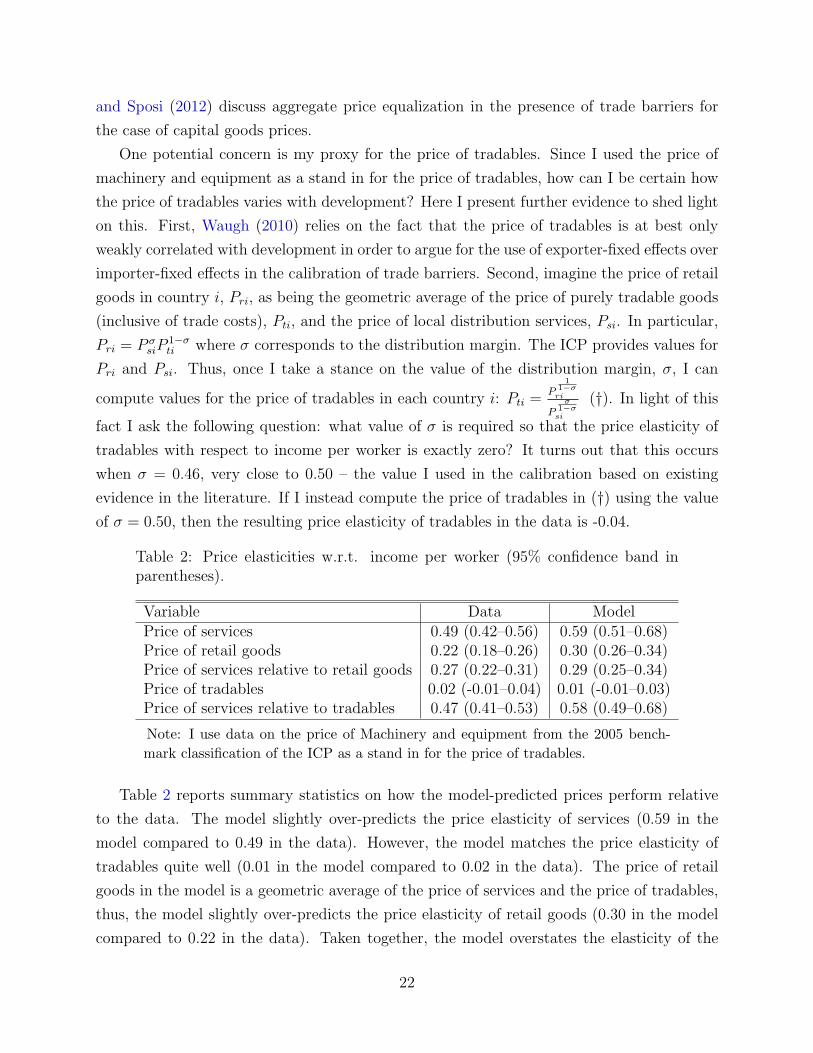
One potential concern is my proxy for the price of tradables. Since I used the price of
machinery and equipment as a stand in for the price of tradables, how can I be certain how
the price of tradables varies with development? Here I present further evidence to shed light
on this. First, Waugh (2010) relies on the fact that the price of tradables is at best only
weakly correlated with development in order to argue for the use of exporter-fixed effects over
importer-fixed effects in the calibration of trade barriers. Second, imagine the price of retail
goods in country i, Pri, as being the geometric average of the price of purely tradable goods
(inclusive of trade costs), Pti, and the price of local distribution services, Psi. In particular,
Pri = P σsiP
1−σti where σ corresponds to the distribution margin. The ICP provides values for
Pri and Psi. Thus, once I take a stance on the value of the distribution margin, σ, I can
compute values for the price of tradables in each country i: Pti =P
11−σ
ri
Pσ
1−σsi
(†). In light of this
fact I ask the following question: what value of σ is required so that the price elasticity of
tradables with respect to income per worker is exactly zero? It turns out that this occurs
when σ = 0.46, very close to 0.50 – the value I used in the calibration based on existing
evidence in the literature. If I instead compute the price of tradables in (†) using the value
of σ = 0.50, then the resulting price elasticity of tradables in the data is -0.04.
Table 2: Price elasticities w.r.t. income per worker (95% confidence band inparentheses).
Variable Data ModelPrice of services 0.49 (0.42–0.56) 0.59 (0.51–0.68)Price of retail goods 0.22 (0.18–0.26) 0.30 (0.26–0.34)Price of services relative to retail goods 0.27 (0.22–0.31) 0.29 (0.25–0.34)Price of tradables 0.02 (-0.01–0.04) 0.01 (-0.01–0.03)Price of services relative to tradables 0.47 (0.41–0.53) 0.58 (0.49–0.68)
Note: I use data on the price of Machinery and equipment from the 2005 bench-mark classification of the ICP as a stand in for the price of tradables.
Table 2 reports summary statistics on how the model-predicted prices perform relative
to the data. The model slightly over-predicts the price elasticity of services (0.59 in the
model compared to 0.49 in the data). However, the model matches the price elasticity of
tradables quite well (0.01 in the model compared to 0.02 in the data). The price of retail
goods in the model is a geometric average of the price of services and the price of tradables,
thus, the model slightly over-predicts the price elasticity of retail goods (0.30 in the model
compared to 0.22 in the data). Taken together, the model overstates the elasticity of the
22

Figure 4: Price of tradables: data and model. I use data on the price of Machinery andequipment from the 2005 benchmark classification of the ICP as a stand in for the price oftradables.
(a) Price of tradables (data).
1/64 1/32 1/16 1/8 1/4 1/2 1 21/4
1/2
1
2
Income per worker: US=1
Price
of
tra
da
ble
s:
US
=1
ALBARG
AUSAUTBEL
BEN
BFA BGD BGR
BOL BRABTN
BWA
CAF CAN
CHECHL
CHN
CIVCMR COL
COM CPV
CYP DNK
ECU
EGY
ESPETH
FIN
FJI
FRAGBRGER
GHA
GIN
GMB
GRC
HKG
HUNIDN
IND
IRL
IRN
ISL
ISRITA
JOR
JPN
KEN
KHM
KOR
LBN
LKA
LUXMAC
MAR
MDG
MDV
MEXMLI MLTMNGMOZ
MRTMUS
MWI
MYS
NAMNLD
NORNZL
OMN
PAKPAN
PER
PHLPOL
PRTPRY
ROMRWA
SAU
SDNSENSGP
STP
SWESWZ
SYR
TGOTHA
TTO
TUN
TUR
TZA
UGAURY
USA
VEN
VNM ZAF
ZMB
slope: 0.02
(b) Price of tradables (model).
1/64 1/32 1/16 1/8 1/4 1/2 1 21/4
1/2
1
2
Income per worker: US=1
Price
of
tra
da
ble
s:
US
=1
ALB
ARG
AUSAUTBEL
BEN
BFA
BGDBGR
BOLBRA
BTN
BWACAF
CANCHE
CHLCHN
CIV
CMR
COLCOM CPVCYP DNK
ECUEGY ESPETH FINFJI FRAGBRGER
GHAGINGMB
GRC
HKGHUN
IDN
IND IRL
IRN
ISLISRITA
JOR JPNKENKHM KOR
LBNLKALUXMAC
MAR
MDG
MDV MEXMLIMLTMNG
MOZ
MRT MUSMWIMYS
NAM
NLDNOR
NZL
OMN
PAK
PAN
PER
PHL
POLPRT
PRY
ROM
RWA
SAU
SDN
SEN
SGP
STP SWE
SWZ
SYR
TGO
THA
TTOTUN
TURTZA
UGA
URY
USA
VEN
VNM ZAF
ZMB
slope:0.01
price of services relative to tradables (0.58 in the model compared to 0.47 in the data), but
replicates the elasticity of the price of services relative to retail goods (0.29 in the model
compared to 0.27 in the data).
Figure 5a plots the model-predicted price of services relative to retail goods against the
corresponding relative price in the data. The countries line up well with the 45-degree
line, indicating that the model captures the systematic differences in relative prices across
countries. Figure 5b plots the model-predicted price of services relative to tradables against
the corresponding relative price in the data. Again, the data are grouped around the 45-
degree line. Figure 6 shows a similar picture for both the absolute price of services as well
as the absolute price of retail goods.
Figure B.3 in appendix B plots average productivity in the tradables sector, (λi/πii)θ,
against income per worker. Average productivity in the tradables sector differs by a factor
of 3.20 between countries in the top decile of the income distribution and countries in the
bottom decile. Productivity in the services sector, Asi, differs by a factor of 1.64 (see table
D.2 in appendix D for a complete list of productivity levels across countries). Together
the calibrated model implies that the productivity gap in tradables between rich and poor
23

Figure 5: Relative price of services: model vs data.
(a) Price of services relative to retail goods.
1/4 1/2 1
1/4
1/2
1
ALB
ARG
AUS
AUT
BEL
BENBFA
BGD
BGR
BOL
BRA
BTN
BWA
CAF
CAN
CHE
CHL
CHNCIV
CMRCOL
COMCPV
CYP
DNK
ECU
EGY
ESP
ETH
FIN
FJI
FRAGBRGER
GHA
GIN
GMB
GRC
HKG
HUN
IDNIND
IRL
IRN
ISLISR ITA
JOR
JPN
KEN
KHM
KOR
LBN
LKA
LUX
MAC
MAR
MDG
MDV
MEX
MLI
MLT
MNG
MOZ
MRT
MUS
MWI
MYS
NAMNLD
NOR
NZL
OMN
PAK
PANPER
PHL
POLPRT
PRY
ROM
RWA
SAU
SDN
SEN
SGP
STP
SWE
SWZ
SYR
TGO
THA
TTO
TUN
TUR
TZA
UGA
URY
USA
VEN
VNM
ZAF
ZMB
Price of services relative to retail goods (data): US=1
Price
of
se
rvic
es r
ela
tive
to
re
tail
go
od
s (
mo
de
l):
US
=1
45o
(b) Price of services relative to tradables.
1/16 1/8 1/4 1/2 1 2
1/16
1/8
1/4
1/2
1
2
ALB
ARG
AUS
AUT
BEL
BENBFA
BGD
BGR
BOL
BRA
BTN
BWA
CAF
CAN
CHE
CHL
CHNCIV
CMRCOL
COMCPV
CYP
DNK
ECU
EGY
ESP
ETH
FIN
FJI
FRAGBRGER
GHA
GIN
GMB
GRC
HKG
HUN
IDNIND
IRL
IRN
ISL
ISR ITA
JOR
JPN
KEN
KHM
KOR
LBN
LKA
LUX
MAC
MAR
MDG
MDV
MEX
MLI
MLT
MNG
MOZ
MRT
MUS
MWI
MYS
NAMNLD
NOR
NZL
OMN
PAK
PANPER
PHL
POL
PRT
PRY
ROM
RWA
SAU
SDN
SEN
SGP
STP
SWE
SWZ
SYR
TGO
THA
TTO
TUN
TUR
TZA
UGA
URY
USA
VEN
VNM
ZAF
ZMB
Price of services relative to tradables (data): US=1
Price
of
se
rvic
es r
ela
tive
to
tra
da
ble
s (
mo
de
l):
US
=1
45o
Figure 6: Prices of services and retail goods: model vs data.
(a) Price of services.
1/16 1/8 1/4 1/2 1 2
1/16
1/8
1/4
1/2
1
2
ALB
ARG
AUS
AUT
BEL
BEN
BFA
BGD
BGR
BOL
BRA
BTN
BWA
CAF
CAN
CHE
CHL
CHN CIVCMR
COL
COMCPV
CYP
DNK
ECU
EGY
ESP
ETH
FIN
FJI
FRAGBRGER
GHA
GIN
GMB
GRC
HKG
HUN
IDN
IND
IRL
IRN
ISL
ISR ITA
JOR
JPN
KEN
KHM
KOR
LBN
LKA
LUX
MAC
MAR
MDG
MDV
MEX
MLI
MLT
MNG
MOZ
MRT
MUS
MWI
MYS
NAM
NLD
NORNZL
OMN
PAK
PANPER
PHL
POL
PRT
PRY
ROM
RWA
SAU
SDN
SEN
SGP
STP
SWE
SWZ
SYR
TGOTHA
TTO
TUN
TUR
TZA
UGA
URY
USA
VEN
VNM
ZAF
ZMB
Price of services (data): US=1
Price
of
se
rvic
es (
mo
de
l):
US
=1
45o
(b) Price of retail goods.
1/4 1/2 1
1/4
1/2
1
ALBARG
AUSAUT
BEL
BEN
BFA
BGD
BGR
BOL
BRA
BTN
BWA
CAF
CAN
CHE
CHL
CHNCIV
CMR
COL
COM
CPV
CYP
DNK
ECU
EGY
ESP
ETH
FIN
FJI
FRAGBRGER
GHA
GIN
GMB
GRC
HKG
HUN
IDN
IND
IRL
IRN
ISL
ISR ITA
JOR
JPN
KEN
KHM
KOR
LBN
LKA
LUX
MAC
MAR
MDG
MDV
MEX
MLI
MLT
MNG
MOZ
MRT
MUS
MWI
MYSNAM
NLD
NORNZL
OMN
PAK
PAN
PER
PHL
POL
PRT
PRY
ROM
RWA
SAU
SDNSEN
SGP
STP
SWE
SWZ
SYR
TGOTHATTO
TUN
TUR
TZA
UGA
URY
USA
VEN
VNM
ZAF
ZMB
Price of retail goods (data): US=1
Price
of
reta
il g
oo
ds (
mo
de
l):
US
=1
45o
24

countries is about twice as large as the productivity gap in services. What’s more is that
measured productivity in the tradables sector in country i depends on the pattern of spe-
cialization through the home trade share πii. Therefore, any policy that alters the set of
goods that a country produces will imply a different average productivity measurement in
the tradables sector.
Labor is more costly in rich countries due to higher productivity in both sectors. Since
there are smaller cross-country productivity differences in the services sector than in the trad-
ables sector, prices of services are higher in rich countries. Crucini, Telmer, and Zachariadis
(2005) argue that this matters primarily to the extent that the share of nontradable inputs
(capital, labor, and services) is sufficiently large. If the share of nontradable inputs in the
production of services was small, then most of the cross-country variation in the price of
services would be due to variation in the price of tradables, which is approximately equal
across countries. In the model, the share of nontradable inputs in the production of services
is indeed large: νs + σs(1 − νs) = 0.87.
A subtle but important implication of my results is that the nontradable input margin
in the production of tradables matters quantitatively only if it occurs after trade has taken
place. If the nontradable margin is applied to tradables after trade occurs (distribution
services in the destination country), then countries where the price of nontradables is high
will systematically face a higher price of retail goods; this effect is discussed in Giri (2012). On
the other hand, if the nontradable margin is applied to production before trade takes place,
i.e., in the producer’s country, then that country’s trading partners will alter their import
shares, and the systematic effect on the composite price of tradables across countries will be
negligible. In the model, the nontradable input margin before trade is νt +σt(1− νt) ∼= 0.43,
while the share of nontradable inputs after trade is σr = 0.50; both numbers are similar in
magnitude. However, there is no systematic variation in the composite price of tradables
across countries, while there is substantial systematic variation in the price of retail goods.
The model slightly over-predicts the price elasticity of services. At least part of the
over-prediction for the price of services can be explained. Consider how I classified goods
as either retail goods or services. The Basic Heading category called “Maintenance and
repair of the dwelling” contains both goods (materials for repair) and services (services for
repair), but I classified this category as services since I can not disaggregate it any further.
There are a few other Basic Headings categories that pose the same issue. Since retail goods
have a lower price elasticity than services, the price elasticity of services that I measured in
the data is likely a lower bound for the true price elasticity of services. It is not possible
to completely avoid this issue so I experimented with other reasonable classifications and I
found that the measured cross-country distributions of prices are practically identical across
25
various classifications.
This measurement issue likely does not explain all of the gap between the model-predicted
price elasticity of services and that in the data. One can also think of other distortions that
affect the prices of domestic goods differently in rich versus poor countries. My focus is
on the quantitative role of trade barriers. As such, with only productivity differences and
asymmetric trade barriers, the model is able to capture a bulk of the systematic variation
in the price data.
My calibration did not use price data to impose any quantitative discipline on the model,
only production and trade data. Thus, the prices generated by the model are a function of
the observed trade and production data. Therefore, I am in a position to ask how relative
prices would look under different distributions of trade barriers, and hence, different patterns
of trade and specialization. This is what I do next.
4.3 Counterfactuals
In the remainder of this section I quantify the importance of trade barriers on relative prices
by examining the implications of changing the pattern of bilateral trade barriers.
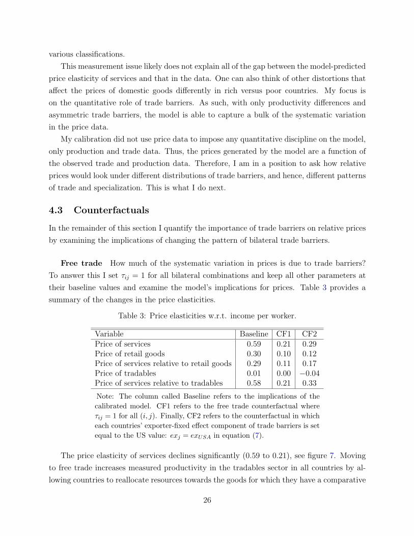
Free trade How much of the systematic variation in prices is due to trade barriers?
To answer this I set τij = 1 for all bilateral combinations and keep all other parameters at
their baseline values and examine the model’s implications for prices. Table 3 provides a
summary of the changes in the price elasticities.
Table 3: Price elasticities w.r.t. income per worker.
Variable Baseline CF1 CF2Price of services 0.59 0.21 0.29Price of retail goods 0.30 0.10 0.12Price of services relative to retail goods 0.29 0.11 0.17Price of tradables 0.01 0.00 −0.04Price of services relative to tradables 0.58 0.21 0.33
Note: The column called Baseline refers to the implications of thecalibrated model. CF1 refers to the free trade counterfactual whereτij = 1 for all (i, j). Finally, CF2 refers to the counterfactual in whicheach countries’ exporter-fixed effect component of trade barriers is setequal to the US value: exj = exUSA in equation (7).
The price elasticity of services declines significantly (0.59 to 0.21), see figure 7. Moving
to free trade increases measured productivity in the tradables sector in all countries by al-
lowing countries to reallocate resources towards the goods for which they have a comparative
26

Figure 7: Price of services: baseline and free trade.
(a) Price of services (baseline).
1/64 1/32 1/16 1/8 1/4 1/2 1 2
1/64
1/32
1/16
1/8
1/4
1/2
1
2
4
8
16
Income per worker: US=1
Price
of
se
rvic
es:
US
=1
ALBARG
AUSAUT
BEL
BEN
BFA
BGD
BGR
BOL
BRA
BTN
BWA
CAF
CAN
CHE
CHL
CHNCIVCMRCOL
COMCPV
CYP
DNK
ECU
EGY
ESP
ETH
FIN
FJI
FRAGBRGER
GHA
GIN
GMB
GRC
HKG
HUN
IDNIND
IRL
IRN
ISLISRITA
JOR
JPN
KENKHM
KOR
LBN
LKA
LUX
MAC
MAR
MDG
MDV
MEX
MLI
MLT
MNGMOZ
MRT
MUS
MWI
MYS
NAM
NLD
NORNZL
OMN
PAK
PANPER
PHL
POLPRT
PRY
ROM
RWA
SAU
SDN
SEN
SGP
STP
SWE
SWZ
SYR
TGO THA
TTO
TUN
TUR
TZA
UGA
URY
USA
VEN
VNM
ZAF
ZMB
slope:0.59
(b) Price of services (free trade).
1/64 1/32 1/16 1/8 1/4 1/2 1 2
1/64
1/32
1/16
1/8
1/4
1/2
1
2
4
8
16
Income per worker: US=1
Price
of
se
rvic
es:
US
=1
ALB
ARG
AUSAUT
BEL
BENBFA
BGD
BGRBOLBRA
BTN
BWA
CAF
CAN
CHE
CHL
CHN
CIVCMR
COL
COM CPV
CYP
DNK
ECU
EGY
ESP
ETH
FINFJI
FRAGBRGER
GHA
GIN
GMB
GRC
HKG
HUN
IDN
IND
IRL
IRN
ISL
ISR
ITAJOR JPN
KENKHM
KOR
LBN
LKA
LUX
MAC
MARMDG
MDV
MEXMLI
MLT
MNGMOZ
MRT MUS
MWI MYS
NAM
NLD
NORNZL
OMN
PAK
PANPER
PHL
POL
PRT
PRY
ROM
RWA SAUSDN
SENSGPSTP
SWE
SWZSYR
TGO
THA
TTO
TUNTUR
TZAUGA
URY
USA
VEN
VNM
ZAF
ZMB
slope:0.21
advantage. This increases the wage rate, and thus increases the price of services. Since poor
countries face larger trade barriers than rich countries do, prices of services increase more
in poor countries than in rich countries. In the free trade counterfactual the 90-10 ratio for
average productivity in tradables is 1.81, while in the baseline model the 90-10 ratio is 3.20,
a magnification of about 80 percent.
PPP holds in the tradables sector since the law of one price applies good by good. Thus,
the price of tradables is equalized across countries and the price elasticity barely changes
(0.01 to 0.00), see figure 8. Notice that although the price elasticity of tradables is essentially
the same in baseline specification and in the free trade counterfactual, in the case of free
trade, tradables prices are identical across countries whereas in the baseline specification,
prices differ across countries but the variation is not systematically related to development.
That is, existing trade barriers do not generate systematic differences in the aggregate price
of tradables across countries. Taken together, the elasticity of the price of services relative
to tradables decreases from 0.58 to 0.21, a reduction of 64 percent.
The change in the price elasticity of retail goods is a weighted average of the change
in the price elasticity of services and the change in the price elasticity of tradables (∆ρr =
σr∆ρs + (1− σr)∆ρt, where ρ is the elasticity). The price elasticity of retail goods decreases
from 0.30 to 0.10.
27

Figure 8: Price of tradables: baseline and free trade.
(a) Price of tradables (baseline).
1/64 1/32 1/16 1/8 1/4 1/2 1 21/4
1/2
1
2
Income per worker: US=1
Price
of
tra
da
ble
s:
US
=1
ALB
ARG
AUSAUTBEL
BEN
BFA
BGDBGR
BOLBRA
BTN
BWACAF
CANCHE
CHLCHN
CIV
CMR
COLCOM CPVCYP DNK
ECUEGY ESPETH FINFJI FRAGBRGER
GHAGINGMB
GRC
HKGHUN
IDN
IND IRL
IRN
ISLISRITA
JOR JPNKENKHM KOR
LBNLKALUXMAC
MAR
MDG
MDV MEXMLIMLTMNG
MOZ
MRT MUSMWIMYS
NAM
NLDNOR
NZL
OMN
PAK
PAN
PER
PHL
POLPRT
PRY
ROM
RWA
SAU
SDN
SEN
SGP
STP SWE
SWZ
SYR
TGO
THA
TTOTUN
TURTZA
UGA
URY
USA
VEN
VNM ZAF
ZMB
slope:0.01
(b) Price of tradables (free trade).
1/64 1/32 1/16 1/8 1/4 1/2 1 21/4
1/2
1
2
Income per worker: US=1
Price
of
tra
da
ble
s:
US
=1
ALB ARG AUSAUTBELBENBFA BGD BGRBOL BRABTN BWACAF CANCHECHLCHNCIVCMR COLCOM CPV CYP DNKECUEGY ESPETH FINFJI FRAGBRGERGHA GINGMB GRCHKGHUNIDNIND IRLIRN ISLISRITAJOR JPNKENKHM KORLBNLKA LUXMACMARMDG MDV MEXMLI MLTMNGMOZMRT MUSMWI MYSNAM NLD NORNZL OMNPAK PANPERPHL POL PRTPRY ROMRWA SAUSDNSEN SGPSTP SWESWZSYRTGO THA TTOTUNTURTZA UGA URY USAVENVNM ZAFZMB
slope:0.00
A complete removal of trade barriers is not meant to be practical: distance cannot be
changed, and there is always going to be a cost associated with geography. However, this
exercise is meant to speak to the role that the mere presence of trade barriers plays in
explaining differences in relative prices. According to the specification that I use to estimate
trade barriers, all of the asymmetry in trade barriers is governed by the exporter-specific
component exj. This suggests that some impediments to trade are indeed specific to each
country and are likely the result of policy or infrastructure, and therefore can potentially
be removed. Next I discuss the implications of removing cross-country differences in the
exporter-specific component only.
Removal of exporter-specific component of trade barriers Recall the parsimo-
nious specification for trade costs given by (7): log τij = γexexj + γdis,kdisij,k + γbrdbrdij +
γlanglangij +εij. The purpose of this exercise is to quantify the importance of the asymmetric
component of the trade barrier that is generated by the exporter-specific fixed effect. The
fact that the exporter-specific fixed effect varies systematically with levels of development
suggests that some component of trade barriers is due to factors other than geography. It is
therefore important to quantify the importance of this channel as it can likely be manipu-
lated by policy. Next I ask, how would relative prices look if the asymmetric component of
28
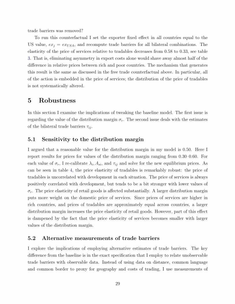
trade barriers was removed?
To run this counterfactual I set the exporter fixed effect in all countries equal to the
US value, exj = exUSA, and recompute trade barriers for all bilateral combinations. The
elasticity of the price of services relative to tradables decreases from 0.58 to 0.33, see table
3. That is, eliminating asymmetry in export costs alone would shave away almost half of the
difference in relative prices between rich and poor countries. The mechanism that generates
this result is the same as discussed in the free trade counterfactual above. In particular, all
of the action is embedded in the price of services; the distribution of the price of tradables
is not systematically altered.
5 Robustness
In this section I examine the implications of tweaking the baseline model. The first issue is
regarding the value of the distribution margin σr. The second issue deals with the estimates
of the bilateral trade barriers τij.
5.1 Sensitivity to the distribution margin
I argued that a reasonable value for the distribution margin in my model is 0.50. Here I
report results for prices for values of the distribution margin ranging from 0.30–0.60. For
each value of σr, I re-calibrate λi, Asi, and τij and solve for the new equilibrium prices. As
can be seen in table 4, the price elasticity of tradables is remarkably robust: the price of
tradables is uncorrelated with development in each situation. The price of services is always
positively correlated with development, but tends to be a bit stronger with lower values of
σr. The price elasticity of retail goods is affected substantially. A larger distribution margin
puts more weight on the domestic price of services. Since prices of services are higher in
rich countries, and prices of tradables are approximately equal across countries, a larger
distribution margin increases the price elasticity of retail goods. However, part of this effect
is dampened by the fact that the price elasticity of services becomes smaller with larger
values of the distribution margin.
5.2 Alternative measurements of trade barriers
I explore the implications of employing alternative estimates of trade barriers. The key
difference from the baseline is in the exact specification that I employ to relate unobservable
trade barriers with observable data. Instead of using data on distance, common language
and common border to proxy for geography and costs of trading, I use measurements of
29

Table 4: Price elasticities w.r.t. income per worker: Re-calibrated modelwith different distribution margin, σr.
Variable data σr = 0.30 σr = 0.40 σr = 0.50 σr = 0.60Price of services 0.49 0.64 0.62 0.59 0.57Price of retail goods 0.22 0.20 0.25 0.30 0.34Price of tradables 0.02 0.01 0.01 0.01 0.01
Note: σr = 0.50 corresponds to the baseline.
transport costs and tariffs. I employ the following specification:
log
(πij
πii
)= F asym
j − F asymi − 1
θβ log(1 + trfi + tcij)︸ ︷︷ ︸
log τasymij
.
I measure transport costs from country j to country i, tcij, by dividing the trade flows in
manufactured goods (from j to i) reported at c.i.f. by the value reported at f.o.b., both
of which come from the Direction of Trade Statistics maintained by the IMF. That is,
tcij =Xcif
ij
Xfobij
− 1. I measure tariffs using applied tariff rate measurements for manufactured
goods for each country i, trfi, from the World Development Indicators database at the World
Bank.10,11 This specification clearly leads to different estimates of the trade barriers, but also
different estimates productivity through the fixed effects Fi.
The implications for prices in this specification are given in table 5. The price elasticity of
services is 0.67, higher than the baseline model (0.59), as well as the data (0.49). Moreover,
the price elasticity of tradables is −0.08, which is further from the data (0.02) compared to
the predictions of the baseline model (0.01). However, the general pattern is a qualitatively
consistent description of the data: a high elasticity of the price of services, and a low (closer
to zero) elasticity of the price of tradables.
In the baseline specification, estimating the matrix of trade barriers requires I + 8 co-
efficients: I country-specific exporter fixed effects, 6 effects from distance intervals, 1 for
common language, and 1 for common border. In this alternative specification estimating
the trade barrier matrix requires only 1 parameter: the parameter on the sum of tariffs
and transport costs. Not surprisingly, the baseline specification out-performs the alternative
specification, mainly because there are more degrees of freedom in matching the trade data.
10The tariff variable for each country i is an average across four different tariff measurements for manufac-tured goods: 1) simple mean, most favored nation, 2) weighted mean, most favored nation, 3) simple mean,all nations, and 4) weighted mean, all nations. Using any one of these tariff measurements individuallyproduces similar results.
11If I simply use the tariff and transport cost data directly to compute trade barriers (i.e, τasymij =
1 + trfi + tcij (i.e., impose β = 1) then the resulting trade barriers will be far to small to reconcile theobserved volume of trade across countries – my estimate of β is 2.04.
30

Table 5: Price elasticities w.r.t. income per worker:Re-calibrated model with alternative estimates fortrade barriers.
Variable Data Baseline AlternativePrice of services 0.49 0.59 0.67Price of retail goods 0.22 0.30 0.29Price of tradables 0.02 0.01 −0.08
Note: The column called Baseline refers to the calibra-tion in which log τij = exj +γdist,kdistij,k +γbrdrbrdrij +γlanglangij + εij . The column called Alternative usesthe following specification for trade barriers: log τij =β log(1 + trfi + tcij).
In turn, the model’s ability to translate the pattern of trade into country-specific prices
speaks to the strength of the model: the closer the calibrated model gets to the trade data,
the closer the model also gets to the price data.
6 Conclusion
I argue that trade barriers are a quantitatively important component in explaining the cross-
country distribution of the relative price of services. The price of services relative to tradables
is determined by the inverse of relative productivity between these two sectors. Trade barriers
help determine the pattern of specialization across multiple, heterogeneous, tradable goods,
which in turn determines measured productivity in the tradables sector.
To formalize this argument I construct a multi-country model of trade with many tradable
goods. Each country’s level of efficiency for each good is a random draw from a country-
specific distribution. Countries differ in their average efficiency across the entire basket of
goods and also face asymmetric bilateral trade barriers. The subset of goods that each
country produces is a function of both average efficiency and trade barriers. Measured
productivity in the tradables sector in turn depends on the set of goods produced.
I calibrate the model to match the observed pattern of bilateral trade as well a cross-
country relative levels of development. The calibration implies three important features: 1)
there are small cross-country productivity differences in services, 2) there are large cross-
country productivity differences in average efficiency in tradables, and 3) poor countries face
larger trade barriers than rich countries do. Larger barriers in poor countries magnify the
disparity in tradables-sector productivity between rich and poor countries, which translates
into large cross-country differences in relative prices. To this end, the model quantitatively
31

replicates the observed distributions of prices: systematically higher prices of services in rich
countries than in poor countries, and the apparent similarity in prices of tradables across
countries. Removing trade barriers eliminates 64 percent of the relative price disparity
between rich and poor countries: the disparity of the price of services between rich and poor
countries shrinks while the disparity of the price of tradables between rich and poor countries
is unchanged.
32

References
Affendy, Arip M, Lau Sim Yee, and Madono Satoru. 2010. “Commodity-industry Classifi-
cation Proxy: A Correspondence Table Between SITC Revision 2 and ISIC Revision 3.”
MPRA Paper 27626, University Library of Munich, Germany.
Alvarez, Fernando and Robert E. Lucas. 2007. “General Equilibrium Analysis of the Eaton-
Kortum Model of International Trade.” Journal of Monetary Economics 54 (6):1726–1768.
Balassa, Bela. 1964. “The Purchasing-Power Parity Doctrine: A Reappraisal.” Journal of
Political Economy 72 (6):584–596.
Barro, Robert J. and Jong-Wha Lee. 2010. “A New Data Set of Educational Attainment in
the World, 19502010.” Working Paper 15902, National Bureau of Economic Research.
Berger, David, Jon Faust, John H. Rogers, and Kai Steverson. 2012. “Border Prices and
Retail Prices.” Journal of International Economics 88 (1):62–73.
Bergin, Paul R., Reuven Glick, and Alan M. Taylor. 2006. “Productivity, Tradability, and
the Long-run Price Puzzle.” Journal of Monetary Economics 53 (8):2041–2066.
Bernard, Andrew B, Jonathan Eaton, J Bradford Jensen, and Samuel Kortum. 2003. “Plants
and Productivity in International Trade.” American Economic Review 93 (4):1268–1290.
Buera, Francisco J., Joseph P. Kaboski, and Yongseok Shin. 2011. “Finance and Develop-
ment: A Tale of Two Sectors.” American Economic Review 101 (5):1964–2002.
Burstein, Ariel, Martin Eichenbaum, and Sergio Rebelo. 2005. “Large Devaluations and the
Real Exchange Rate.” Journal of Political Economy 113 (4):742–784.
Burstein, Ariel, Joao C. Neves, and Sergio Rebelo. 2004. “Investment Prices and Exchange
Rates: Some Basic Facts.” NBER Working Papers 10238, National Bureau of Economic
Research, Inc.
Burstein, Ariel T., Joao C. Neves, and Sergio Rebelo. 2003. “Distribution Costs and Real
Exchange Rate Dynamics During Exchange-Rate-Based Stabilizations.” Journal of Mon-
etary Economics 50 (6):1189–1214.
Caselli, Francesco. 2005. “Accounting for Cross-Country Income Differences.” In Handbook of
Economic Growth, edited by Philippe Aghion and Steven Durlauf, Handbook of Economic
Growth, chap. 9. Elsevier, 679–741.
33

Crucini, Mario J., Chris I. Telmer, and Marios Zachariadis. 2005. “Understanding European
Real Exchange Rates.” American Economic Review 95 (3):724–738.
Crucini, Mario J. and Hakan Yilmazkuday. 2009. “A Model of International Cities: Impli-
cations for Real Exchange Rates.” Working Paper 14834, National Bureau of Economic
Research.
Djankov, Simeon, Caroline Freund, and Cong S. Pham. 2006. “Trading on time.” Policy
Research Working Paper Series 3909, The World Bank.
Eaton, Jonathan and Samuel Kortum. 2001. “Trade in Capital Goods.” European Economic
Review 45:1195–1235.
———. 2002. “Technology, Geography, and Trade.” Econometrica 70 (5):1741–1779.
Giri, Rahul. 2012. “Local Costs of Distribution, International Trade Costs and Micro Evi-
dence on the Law of One Price.” Journal of International Economics 86 (1):82–100.
Gollin, Douglas. 2002. “Getting Income Shares Right.” Journal of Political Economy
110 (2):458–474.
Hall, Robert E. and Charles I. Jones. 1999. “Why Do Some Countries Produce So Much
More Output per Worker than Others?” Quarterly Journal of Economics 114 (1):83–116.
Herrendorf, Berthold and Akos Valentinyi. 2012. “Which Sectors Make Poor Countries So
Unproductive?” Journal of the European Economic Association 10 (2):323–341.
Heston, Alan, Daniel A. Nuxoll, and Robert Summers. 1994. “The Differential-Productivity
Hypothesis and Purchasing-Power Parities: Some New Evidence.” Review of Inernational
Economics 2 (3):227–243.
Heston, Alan, Robert Summers, and Bettina Aten. 2009. “Penn World Table Version 6.3.”
Center for International Comparisons of Production, Income and Prices at the University
of Pennsylvania.
Hsieh, Chang-Tai and Peter J. Klenow. 2007. “Relative Prices and Relative Prosperity.”
American Economic Review 97 (3):562–585.
Hummels, David. 2001. “Time as a Trade Barrier.” GTAP Working Papers 1152, Center
for Global Trade Analysis, Department of Agricultural Economics, Purdue University.
34

Kravis, Irving B. and Robert E. Lipsey. 1988. “National Price Levels and the Prices of Trad-
ables and Nontradables.” American Economic Review: Papers and Proceedings 78 (2):474–
478.
Li, Yue and S. Wilson. 2009. “Time as a Determinant of Comparative Advantage.” Policy
Research Working Paper 5128, World Bank, Devlopement Research Group, Trade and
Integration Team.
Marquez, Jaime, Charles Thomas, and Corinne Land. 2012. “International Relative Price
Levels: A Look Under the Hood.” International Finance Discussion Papers 1055, Board
of Governors of the Federal Reserve System (U.S.).
Mutreja, Piyusha, B. Ravikumar, Raymond Riezman, and Michael Sposi. 2012. “Price
Equalization Does Not Imply Free Trade.” Globalization and Monetary Policy Institute
Working Paper 129, Federal Reserve Bank of Dallas.
Restuccia, Diego and Carlos Urrutia. 2001. “Relative Prices and Investment Rates.” Journal
of Monetary Economics 47 (1):93–121.
Samuelson, Paul A. 1964. “Theoretical Notes on Trade Problems.” Review of Economics
and Statistics 46 (2):145–154.
Simonovska, Ina. 2010. “Income Differences and Prices of Tradables.” NBER Working
Papers 16233, National Bureau of Economic Research, Inc.
Simonovska, Ina and Michael E. Waugh. 2010. “The Elasticity of Trade: Estimates &
Evidence.” CAGE Online Working Paper Series 13, Competitive Advantage in the Global
Economy (CAGE).
UNIDO. 2010. International Yearbook of Industrial Statistics 2010. Edward Elgar Publishing.
Waugh, Michael E. 2010. “International Trade and Income Differences.” American Economic
Review 100 (5):2093–2124.
35

A Data
This section describes my data sources as well as how I map the model to the data.
Categories I identify tradables with categories 15**-37** according to the four-digit
ISIC revision 3 classification (see http://unstats.un.org/unsd/cr/registry/regcst.asp?cl=2).
I interpret retail goods as the same inherent goods as tradables, the difference being that
retail goods are the transformation of tradable goods from the dock to the final consumer.
Prices and expenditures I use detailed retail data collected by the ICP at the Basic
Headings level for the year 2005. I classify each Basic Headings category as either services or
goods by using my own correspondence given in table D.1 in appendix D (recall that retail
goods are the same as tradable goods; retail goods just include a distribution margin). Some
categories are labeled as N/A as they do not pertain to any particular type of good, i.e.,
the category called “Gross operating surplus”. The ICP records prices and expenditures in
local currency for a common basket of goods across countries at the retail level. I construct
country-specific prices for retail goods and services for each country as follows. Let B denote
a basket of Basic Heading categories, either retail goods or services. Each element b ∈ B is
a Basic Heading category. The ICP provides data on expenditures in local currency on each
category b, which I convert into 2005 US dollars using the nominal exchange rate. I denote
country i’s total expenditures in US dollars as EXP dombi . Similarly, the ICP provides prices
in local currency for each category b. For each country i I convert the price of each category b
into US dollars using the exchange rate and denote this price as PPPbi. I construct country
i’s expenditures in international dollars for each category b as EXP intbi =
EXP dombi
PPPbi. I compute
the aggregate PPP price in country i for the entire basket B by dividing expenditures in US
dollars by expenditures in international dollars: Pbi =∑
b∈B EXP dombi∑
b∈B EXP intbi
.
Human Capital I use data on years of schooling from Barro and Lee (2010) to con-
struct human capital measures. I take average years of schooling for the population age 25
and up and convert into measures of human capital using h = exp(ϕ(s)), where ϕ is piecewise
linear in average years of schooling s. This method is identical to the one used by Hall and
Jones (1999) and Caselli (2005).
National Accounts Real income per worker is taken directly from PWT63 as the
variable rgdpwok. The size of the workforce is constructed using PWT63 data as follows:
number of workers equals 1000*pop*rgdpl/rgdpwok. I use the perpetual inventory method
36

to construct aggregate stocks of capital:
Kt+1 = It + (1 − δ)Kt,
where It is aggregate investment in PPP and δ is the depreciation rate. It computed from
PWT63 as rgdpl*pop*ki. The initial capital stock K0 is computed as I0/(g + δ), where
I0 is the value of the investment series in the first year it is available, and g is the average
geometric growth rate for the investment series between the first year with available data
and 1975 (for some countries the first year with available data is after 1975, In which case,
the geometric growth rate for first 5 years with available data is calculated). Following the
literature, δ is set to 0.06.
Production Data on tradables production is taken from INDSTAT4, a database main-
tained by UNIDO at the four-digit ISIC revision 3 level. I compute gross production as the
sum of gross output over all tradable categories.
Trade barriers Trade barriers are assumed to be a function of distance, common
language, and shared border; each of which are taken from Centre D’Etudes Prospectives Et
D’Informations Internationales (http://www.cepii.fr/welcome.htm).
Trade Flows Data on bilateral trade flows are obtained from UN Comtrade for the
year 2005 (http://comtrade.un.org/). All trade flow data is at the four-digit SITC revision
2 level, and then aggregated into total trade flows. In order to link trade data to production
data I employ the correspondence provided by Affendy, Sim Yee, and Satoru (2010) which
links ISIC revision 3 to SITC revision 2 at the 4 digit level.
Construction of Trade Shares The empirical counterpart to the model variable πij
is constructed following Bernard, Eaton, Jensen, and Kortum (2003) (recall that this is the
fraction of country i’s spending on tradables that was purchased from country j). I divide
the value of country i’s imports of tradables from country j, by i’s gross production of
tradables minus i’s total exports of tradables (to the rest of the world) plus i’s total imports
of tradables (from only countries in my sample) to arrive at the bilateral trade share.
B Additional figures
This appendix provides additional figures that are referenced in the main body of the text.
37
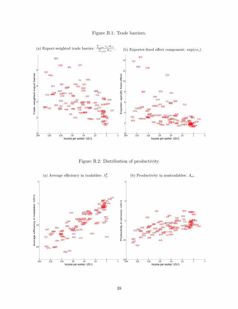
Figure B.1: Trade barriers.
(a) Export-weighted trade barrier:∑
j =i τjiXji∑j =i Xji
.
1/64 1/32 1/16 1/8 1/4 1/2 1 20
2
4
6
8
ALB
ARG
AUS
AUT
BEL
BEN
BFA
BGD
BGR
BOL
BRA
BTN
BWA
CAF
CAN
CHE
CHL
CHN
CIV
CMR
COL
COM
CPV
CYPDNK
ECU
EGY
ESP
ETH
FIN
FJI
FRAGBR
GER
GHA GIN
GMB
GRC
HKG
HUN
IDN
IND
IRL
IRN
ISL
ISR
ITA
JOR
JPN
KEN
KHM
KOR
LBN
LKA
LUX
MAC
MARMDG
MDV
MEX
MLI
MLTMNGMOZ
MRT
MUS
MWIMYSNAM
NLDNOR
NZL
OMN
PAK
PAN
PER
PHLPOL
PRTPRYROM
RWA
SAU
SDN
SEN
SGP
STP
SWE
SWZ
SYR
TGO
THA
TTO
TUN
TUR
TZA
UGAURY
USAVEN
VNM ZAF
ZMB
Income per worker: US=1
Tra
de
−w
eig
hte
d e
xp
ort
ba
rrie
r
(b) Exporter-fixed effect component: exp(exi).
1/64 1/32 1/16 1/8 1/4 1/2 1 20
2
4
6
8
10
12
14
ALB
ARGAUSAUT
BEL
BEN
BFA
BGD BGR
BOL
BRA
BTN
BWA
CAF
CANCHECHL
CHN
CIV
CMR
COL
COM
CPV
CYP
DNK
ECU
EGY
ESP
ETH
FIN
FJI
FRAGBRGER
GHA
GIN
GMB
GRC
HKG
HUN
IDNIND IRL
IRNISL
ISR
ITA
JOR
JPN
KENKHM
KOR
LBNLKA
LUXMACMAR
MDG
MDV
MEX
MLI MLTMNG
MOZ
MRT
MUSMWI
MYS
NAM
NLD
NORNZL
OMN
PAK PAN
PER
PHLPOL
PRT
PRY
ROM
RWA
SAU
SDN
SEN
SGP
STP
SWE
SWZ
SYR
TGO
THA
TTO
TUN
TUR
TZA
UGA
URY
USA
VEN
VNM ZAF
ZMB
Income per worker: US=1
Exp
ort
er−
sp
ecific
fix
ed
eff
ect
Figure B.2: Distribution of productivity.
(a) Average efficiency in tradables: λθi .
1/64 1/32 1/16 1/8 1/4 1/2 1 2
1/4
1/2
1
2
ALB
ARG
AUS
AUT
BEL
BEN
BFA
BGD
BGR
BOL
BRA
BTN
BWA
CAF
CANCHE
CHL
CHN
CIVCMR
COL
COM
CPV
CYPDNK
ECU
EGY
ESP
ETH
FIN
FJI
FRAGBR
GER
GHA
GIN
GMB
GRC
HKG
HUN
IDNIND
IRL
IRN
ISL
ISRITA
JOR
JPN
KENKHM
KORLBN
LKA
LUX
MAC
MAR
MDG
MDV
MEX
MLI
MLT
MNG
MOZ
MRT
MUS
MWI
MYS
NAM
NLD
NOR
NZL
OMN
PAK
PAN
PER
PHL
POLPRT
PRY
ROM
RWA
SAU
SDN
SEN
SGP
STP
SWE
SWZ
SYR
TGO
THA
TTO
TUN
TUR
TZA
UGA
URY
USA
VEN
VNM
ZAF
ZMB
Income per worker: US=1
Avera
ge e
ffic
iency in tra
dable
s: U
S=
1
(b) Productivity in nontradables: Asi.
1/64 1/32 1/16 1/8 1/4 1/2 1 21/4
1/2
1
2
4
ALB
ARG
AUSAUT
BEL
BENBFA
BGDBGR
BOL
BRA
BTN
BWA
CAF
CANCHE
CHL
CHNCIV
CMRCOL
COM
CPV
CYP DNK
ECU
EGY
ESP
ETH
FIN
FJI
FRAGBR
GER
GHA
GIN
GMB
GRC
HKG
HUN
IDNIND
IRL
IRN
ISLISR
ITA
JORJPN
KEN
KHM KORLBN
LKALUX
MAC
MAR
MDG
MDV
MEXMLI MLT
MNG
MOZ
MRT
MUS
MWI
MYS
NAM
NLD
NOR
NZL
OMN
PAK
PANPER
PHLPOL
PRT
PRY
ROM
RWA
SAU
SDN
SEN
SGP
STP
SWE
SWZ
SYR
TGO
THATTO
TUN
TUR
TZA
UGA
URYUSA
VENVNM
ZAF
ZMB
Income per worker: US=1
Pro
ductivity in s
erv
ices: U
S=
1
38

Figure B.3: Average productivity in tradables:(
λi
πii
)θ
.
1/64 1/32 1/16 1/8 1/4 1/2 1 2
1/4
1/2
1
2
ALBARG
AUS
AUT
BEL
BEN
BFA
BGD
BGR
BOL
BRA
BTN
BWA
CAF
CAN
CHE
CHL
CHNCIVCMR
COL
COM
CPV
CYP
DNK
ECU
EGY
ESP
ETH
FIN
FJI
FRAGBRGER
GHA
GIN
GMB
GRC
HKGHUN
IDNIND
IRL
IRN
ISL
ISR
ITA
JOR
JPN
KENKHM
KOR
LBN
LKA
LUX
MAC
MAR
MDG
MDV
MEX
MLI
MLT
MNG
MOZ
MRT
MUS
MWI
MYSNAM
NLD
NOR
NZL
OMN
PAK
PANPER
PHL
POL
PRT
PRY
ROM
RWA
SAU
SDN
SEN
SGP
STP
SWE
SWZ
SYR
TGO
THA
TTO
TUN
TUR
TZA
UGA
URY
USA
VEN
VNM
ZAF
ZMB
Income per worker: US=1
Ave
rage
pro
duct
ivity
in tr
adab
les
US
=1
Figure B.4: Income per worker: model vs data. The only margin of error for income perworker between the model and the data comes from the difference in home trade shares, πii,between the model and the data – I did not directly target home trade shares.
1/64 1/32 1/16 1/8 1/4 1/2 1
1/64
1/32
1/16
1/8
1/4
1/2
1
ALB
ARG
AUSAUTBEL
BENBFA
BGD
BGR
BOL
BRA
BTN
BWA
CAF
CANCHE
CHL
CHN
CIVCMR
COL
COM
CPV
CYP
DNK
ECU
EGY
ESP
ETH
FIN
FJI
FRAGBRGER
GHA
GIN
GMB
GRC
HKG
HUN
IDNIND
IRL
IRN
ISLISR
ITA
JOR
JPN
KENKHM
KOR
LBN
LKA
LUX
MAC
MAR
MDG
MDV
MEX
MLI
MLT
MNG
MOZMRT
MUS
MWI
MYS
NAM
NLD
NOR
NZLOMN
PAK
PAN
PER
PHL
POL
PRT
PRY
ROM
RWA
SAU
SDN
SEN
SGP
STP
SWE
SWZ
SYR
TGO
THA
TTO
TUNTUR
TZA
UGA
URY
USA
VEN
VNM
ZAF
ZMB
Income per worker (data): US=1
Inco
me
per w
orke
r (m
odel
): U
S=1
45o
39
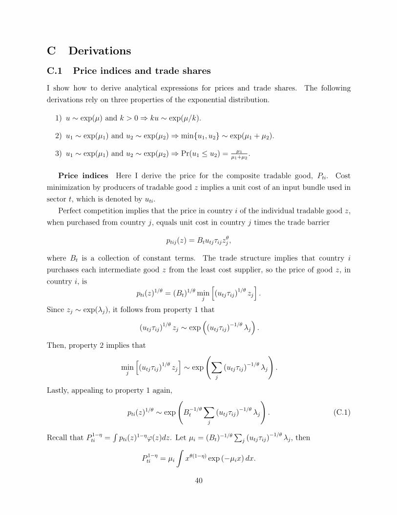
C Derivations
C.1 Price indices and trade shares
I show how to derive analytical expressions for prices and trade shares. The following
derivations rely on three properties of the exponential distribution.
1) u ∼ exp(µ) and k > 0 ⇒ ku ∼ exp(µ/k).
2) u1 ∼ exp(µ1) and u2 ∼ exp(µ2) ⇒ minu1, u2 ∼ exp(µ1 + µ2).
3) u1 ∼ exp(µ1) and u2 ∼ exp(µ2) ⇒ Pr(u1 ≤ u2) = µ1
µ1+µ2.
Price indices Here I derive the price for the composite tradable good, Pti. Cost
minimization by producers of tradable good z implies a unit cost of an input bundle used in
sector t, which is denoted by uti.
Perfect competition implies that the price in country i of the individual tradable good z,
when purchased from country j, equals unit cost in country j times the trade barrier
ptij(z) = Btutjτijzθj ,
where Bt is a collection of constant terms. The trade structure implies that country i
purchases each intermediate good z from the least cost supplier, so the price of good z, in
country i, is
pti(z)1/θ = (Bt)1/θ min
j
[(utjτij)
1/θ zj
].
Since zj ∼ exp(λj), it follows from property 1 that
(utjτij)1/θ zj ∼ exp
((utjτij)
−1/θ λj
).
Then, property 2 implies that
minj
[(utjτij)
1/θ zj
]∼ exp
(∑j
(utjτij)−1/θ λj
).
Lastly, appealing to property 1 again,
pti(z)1/θ ∼ exp
(B
−1/θt
∑j
(utjτij)−1/θ λj
). (C.1)
Recall that P 1−ηti =
∫pti(z)1−ηφ(z)dz. Let µi = (Bt)
−1/θ∑
j (utjτij)−1/θ λj, then
P 1−ηti = µi
∫xθ(1−η) exp (−µix) dx.
40
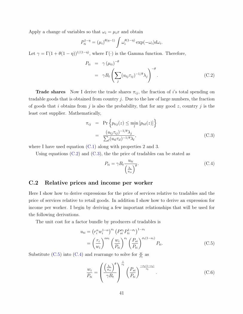
Apply a change of variables so that ωi = µix and obtain
P 1−ηti = (µi)
θ(η−1)
∫ω
θ(1−η)i exp(−ωi)dωi.
Let γ = Γ(1 + θ(1 − η))1/(1−η), where Γ(·) is the Gamma function. Therefore,
Pti = γ (µti)−θ
= γBt
(∑j
(utjτij)−1/θλj
)−θ
. (C.2)
Trade shares Now I derive the trade shares πij, the fraction of i’s total spending on
tradable goods that is obtained from country j. Due to the law of large numbers, the fraction
of goods that i obtains from j is also the probability, that for any good z, country j is the
least cost supplier. Mathematically,
πij = Pr
ptij(z) ≤ minl
[ptil(z)]
=(utjτij)
−1/θλj∑l(utlτil)−1/θλl
, (C.3)
where I have used equation (C.1) along with properties 2 and 3.
Using equations (C.2) and (C.3), the the price of tradables can be stated as
Pti = γBtuti(λi
πii
)θ. (C.4)
C.2 Relative prices and income per worker
Here I show how to derive expressions for the price of services relative to tradables and the
price of services relative to retail goods. In addition I show how to derive an expression for
income per worker. I begin by deriving a few important relationships that will be used for
the following derivations.
The unit cost for a factor bundle by producers of tradables is
uti =(rαi w1−α
i
)νt(P σt
si P 1−σtti
)1−νt
=
(ri
wi
)ανt(
wi
Pti
)νt(
Psi
Pti
)σt(1−νt)
Pti. (C.5)
Substitute (C.5) into (C.4) and rearrange to solve for wPt
as
wi
Pti
=
(
λi
πii
)θ
γBt
1νt (
Psi
Pti
)−σt(1−νt)νt
. (C.6)
41
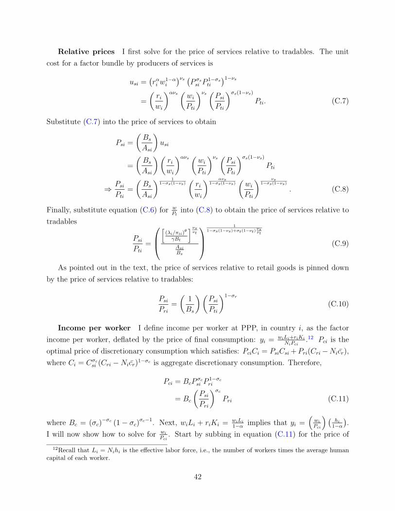
Relative prices I first solve for the price of services relative to tradables. The unit
cost for a factor bundle by producers of services is
usi =(rαi w1−α
i
)νs(P σs
si P 1−σsti
)1−νs
=
(ri
wi
)ανs(
wi
Pti
)νs(
Psi
Pti
)σs(1−νs)
Pti. (C.7)
Substitute (C.7) into the price of services to obtain
Psi =
(Bs
Asi
)usi
=
(Bs
Asi
)(ri
wi
)ανs(
wi
Pti
)νs(
Psi
Pti
)σs(1−νs)
Pti
⇒ Psi
Pti
=
(Bs
Asi
) 11−σs(1−νs)
(ri
wi
) ανs1−σs(1−νs)
(wi
Pti
) νs1−σs(1−νs)
. (C.8)
Finally, substitute equation (C.6) for wPt
into (C.8) to obtain the price of services relative to
tradables
Psi
Pti
=
[
(λi/πii)θ
γBt
] νsνt
Asi
Bs
1
1−σs(1−νs)+σt(1−νt)νsνt
(C.9)
As pointed out in the text, the price of services relative to retail goods is pinned down
by the price of services relative to tradables:
Psi
Pri
=
(1
Bs
)(Psi
Pti
)1−σr
(C.10)
Income per worker I define income per worker at PPP, in country i, as the factor
income per worker, deflated by the price of final consumption: yi = wiLi+riKi
NiPci.12 Pci is the
optimal price of discretionary consumption which satisfies: PciCi = PsiCsi + Pri(Cri −Nicr),
where Ci = Cσcsi (Cri − Nicr)
1−σc is aggregate discretionary consumption. Therefore,
Pci = BcPσcsi P 1−σc
ri
= Bc
(Psi
Pri
)σc
Pri (C.11)
where Bc = (σc)−σc (1 − σc)
σc−1. Next, wiLi + riKi = wiLi
1−αimplies that yi =
(wi
Pci
) (hi
1−α
).
I will now show how to solve for wi
Pci. Start by subbing in equation (C.11) for the price of
12Recall that Li = Nihi is the effective labor force, i.e., the number of workers times the average humancapital of each worker.
42
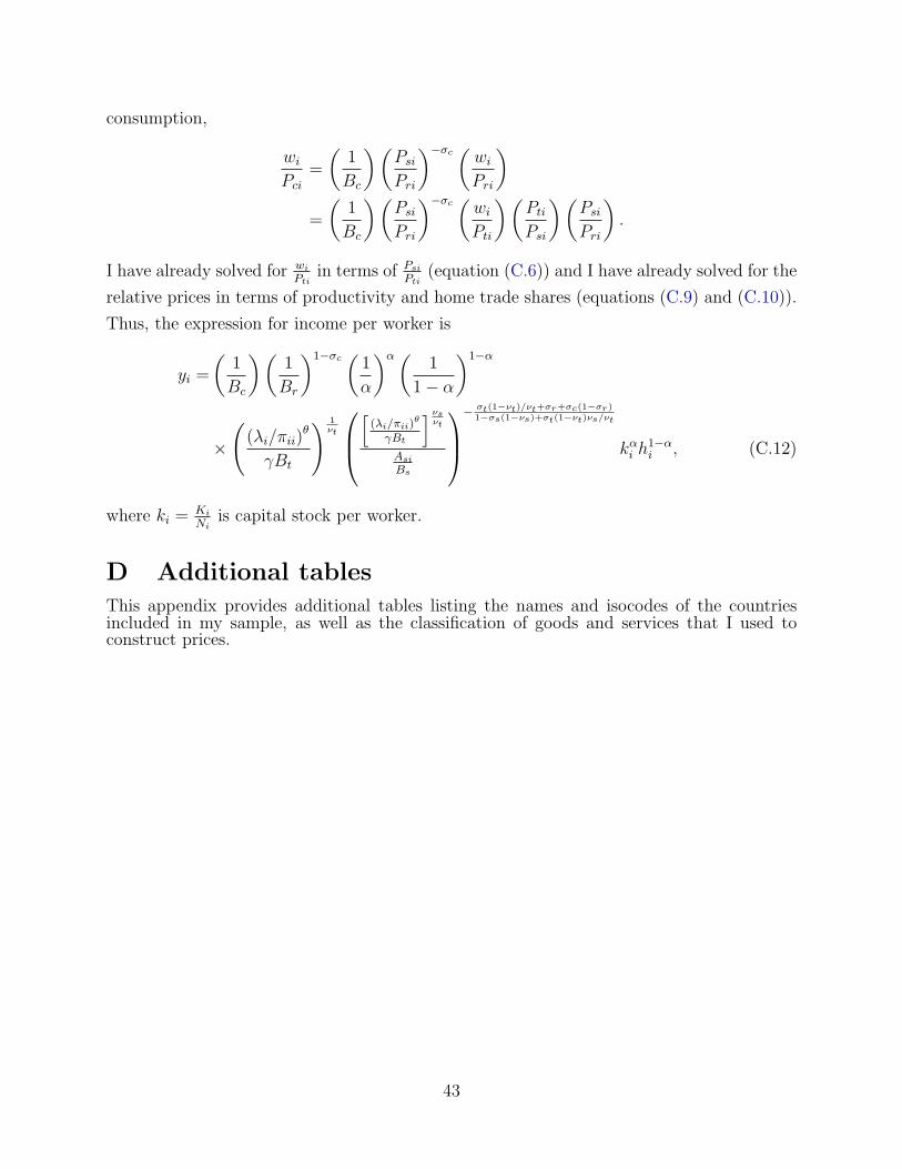
consumption,
wi
Pci
=
(1
Bc
)(Psi
Pri
)−σc(
wi
Pri
)=
(1
Bc
)(Psi
Pri
)−σc(
wi
Pti
)(Pti
Psi
)(Psi
Pri
).
I have already solved for wi
Ptiin terms of Psi
Pti(equation (C.6)) and I have already solved for the
relative prices in terms of productivity and home trade shares (equations (C.9) and (C.10)).
Thus, the expression for income per worker is
yi =
(1
Bc
)(1
Br
)1−σc(
1
α
)α(1
1 − α
)1−α
×
((λi/πii)
θ
γBt
) 1νt
[
(λi/πii)θ
γBt
] νsνt
Asi
Bs
− σt(1−νt)/νt+σr+σc(1−σr)
1−σs(1−νs)+σt(1−νt)νs/νt
kαi h1−α
i , (C.12)
where ki = Ki
Niis capital stock per worker.
D Additional tablesThis appendix provides additional tables listing the names and isocodes of the countriesincluded in my sample, as well as the classification of goods and services that I used toconstruct prices.
43
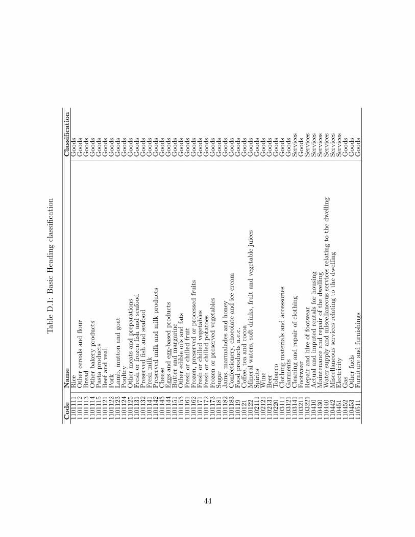
Tab
leD
.1:
Bas
icH
eadin
gcl
assi
fica
tion
Code
Nam
eC
lass
ifica
tion
1101
111
Ric
eG
oods
1101
112
Oth
erce
real
san
dflo
urG
oods
1101
113
Bre
adG
oods
1101
114
Oth
erba
kery
prod
ucts
Goo
ds11
0111
5Pas
tapr
oduc
tsG
oods
1101
121
Bee
fan
dve
alG
oods
1101
122
Por
kG
oods
1101
123
Lam
b,m
utto
nan
dgo
atG
oods
1101
124
Pou
ltry
Goo
ds11
0112
5O
ther
mea
tsan
dpr
epar
atio
nsG
oods
1101
131
Fres
hor
froz
enfis
han
dse
afoo
dG
oods
1101
132
Pre
serv
edfis
han
dse
afoo
dG
oods
1101
141
Fres
hm
ilkG
oods
1101
142
Pre
serv
edm
ilkan
dm
ilkpr
oduc
tsG
oods
1101
143
Che
ese
Goo
ds11
0114
4E
ggs
and
egg-
base
dpr
oduc
tsG
oods
1101
151
But
ter
and
mar
gari
neG
oods
1101
153
Oth
ered
ible
oils
and
fats
Goo
ds11
0116
1Fr
esh
orch
illed
frui
tG
oods
1101
162
Froz
en,pr
eser
ved
orpr
oces
sed
frui
tsG
oods
1101
171
Fres
hor
chill
edve
geta
bles
Goo
ds11
0117
2Fr
esh
orch
illed
pota
toes
Goo
ds11
0117
3Fr
ozen
orpr
eser
ved
vege
tabl
esG
oods
1101
181
Suga
rG
oods
1101
182
Jam
s,m
arm
alad
esan
dho
ney
Goo
ds11
0118
3C
onfe
ctio
nery
,ch
ocol
ate
and
ice
crea
mG
oods
1101
19Fo
odpr
oduc
tsn.
e.c.
Goo
ds11
0121
Coff
ee,te
aan
dco
coa
Goo
ds11
0122
Min
eral
wat
ers,
soft
drin
ks,fr
uit
and
vege
tabl
eju
ices
Goo
ds11
0211
1Sp
irit
sG
oods
1102
121
Win
eG
oods
1102
131
Bee
rG
oods
1102
20Tob
acco
Goo
ds11
0311
1C
loth
ing
mat
eria
lsan
dac
cess
orie
sG
oods
1103
121
Gar
men
tsG
oods
1103
141
Cle
anin
gan
dre
pair
ofcl
othi
ngSe
rvic
es11
0321
1Fo
otw
ear
Goo
ds11
0322
1R
epai
ran
dhi
reof
foot
wea
rSe
rvic
es11
0410
Act
ualan
dim
pute
dre
ntal
sfo
rho
usin
gSe
rvic
es11
0430
Mai
nten
ance
and
repa
irof
the
dwel
ling
Serv
ices
1104
40W
ater
supp
lyan
dm
isce
llane
ous
serv
ices
rela
ting
toth
edw
ellin
gSe
rvic
es11
0442
Mis
cella
neou
sse
rvic
esre
lati
ngto
the
dwel
ling
Serv
ices
1104
51E
lect
rici
tySe
rvic
es11
0452
Gas
Goo
ds11
0453
Oth
erfu
els
Goo
ds11
0511
Furn
itur
ean
dfu
rnis
hing
sG
oods
44

Tab
leD
.1–
Con
tinu
ed
Code
Nam
eC
lass
ifica
tion
1105
12C
arpe
tsan
dot
her
floor
cove
ring
sG
oods
1105
13R
epai
rof
furn
itur
e,fu
rnis
hing
san
dflo
orco
veri
ngs
Serv
ices
1105
20H
ouse
hold
text
iles
Goo
ds11
0531
Maj
orho
useh
old
appl
ianc
esw
heth
erel
ectr
icor
not
Goo
ds11
0532
Smal
lel
ectr
icho
useh
old
appl
ianc
esG
oods
1105
33R
epai
rof
hous
ehol
dap
plia
nces
Serv
ices
1105
40G
lass
war
e,ta
blew
are
and
hous
ehol
dut
ensi
lsG
oods
1105
51M
ajor
tool
san
deq
uipm
ent
Goo
ds11
0552
Smal
lto
ols
and
mis
cella
neou
sac
cess
orie
sG
oods
1105
61N
on-d
urab
leho
useh
old
good
sG
oods
1105
621
Dom
esti
cse
rvic
esSe
rvic
es11
0562
2H
ouse
hold
serv
ices
Serv
ices
1106
11P
harm
aceu
tica
lpr
oduc
tsG
oods
1106
12O
ther
med
ical
prod
ucts
Goo
ds11
0613
The
rape
utic
alap
plia
nces
and
equi
pmen
tG
oods
1106
21M
edic
alSe
rvic
esSe
rvic
es11
0622
Den
talse
rvic
esSe
rvic
es11
0623
Par
amed
ical
serv
ices
Serv
ices
1106
30H
ospi
talse
rvic
esSe
rvic
es11
0711
Mot
orca
rsG
oods
1107
12M
otor
cycl
esG
oods
1107
13B
icyc
les
Goo
ds11
0722
Fuel
san
dlu
bric
ants
for
pers
onal
tran
spor
teq
uipm
ent
Goo
ds11
0723
Mai
nten
ance
and
repa
irof
pers
onal
tran
spor
teq
uipm
ent
Serv
ices
1107
24O
ther
serv
ices
inre
spec
tof
pers
onal
tran
spor
teq
uipm
ent
Serv
ices
1107
31Pas
seng
ertr
ansp
ort
byra
ilway
Serv
ices
1107
32Pas
seng
ertr
ansp
ort
byro
adSe
rvic
es11
0733
Pas
seng
ertr
ansp
ort
byai
rSe
rvic
es11
0734
Pas
seng
ertr
ansp
ort
byse
aan
din
land
wat
erw
aySe
rvic
es11
0735
Com
bine
dpa
ssen
ger
tran
spor
tSe
rvic
es11
0736
Oth
erpu
rcha
sed
tran
spor
tse
rvic
esSe
rvic
es11
0810
Pos
talse
rvic
esSe
rvic
es11
0820
Tel
epho
nean
dte
lefa
xeq
uipm
ent
Goo
ds11
0830
Tel
epho
nean
dte
lefa
xse
rvic
esSe
rvic
es11
0911
Aud
io-v
isua
l,ph
otog
raph
ican
din
form
atio
npr
oces
sing
equi
pmen
tG
oods
1109
14R
ecor
ding
med
iaG
oods
1109
15R
epai
rof
audi
o-vi
sual
,ph
otog
raph
ican
din
form
atio
npr
oces
sing
equi
pmen
tSe
rvic
es11
0921
Maj
ordu
rabl
esfo
rou
tdoo
ran
din
door
recr
eati
onG
oods
1109
31O
ther
recr
eati
onal
item
san
deq
uipm
ent
Goo
ds11
0933
Gar
dens
and
pets
Serv
ices
1109
35V
eter
inar
yan
dot
her
serv
ices
for
pets
Serv
ices
1109
41R
ecre
atio
nalan
dsp
orti
ngse
rvic
esSe
rvic
es11
0942
Cul
tura
lse
rvic
esSe
rvic
es11
0943
Gam
esof
chan
ceG
oods
1109
50N
ewsp
aper
s,bo
oks
and
stat
ione
ryG
oods
1109
60Pac
kage
holid
ays
Serv
ices
1110
00E
duca
tion
Serv
ices
45

Tab
leD
.1–
Con
tinu
ed
Code
Nam
eC
lass
ifica
tion
1111
10C
ater
ing
serv
ices
Serv
ices
1111
20A
ccom
mod
atio
nse
rvic
esSe
rvic
es11
1211
Hai
rdre
ssin
gsa
lons
and
pers
onal
groo
min
ges
tabl
ishm
ents
Serv
ices
1112
12A
pplia
nces
,ar
ticl
esan
dpr
oduc
tsfo
rpe
rson
alca
reG
oods
1112
20P
rost
itut
ion
Serv
ices
1112
31Je
wel
ery,
cloc
ksan
dw
atch
esG
oods
1112
32O
ther
pers
onal
effec
tsG
oods
1112
40So
cial
prot
ecti
onSe
rvic
es11
1250
Insu
ranc
eSe
rvic
es11
1261
FIS
IMSe
rvic
es11
1262
Oth
erfin
anci
alse
rvic
esn.
e.c
Serv
ices
1112
70O
ther
serv
ices
n.e.
c.Se
rvic
es11
1300
Net
purc
hase
sab
road
N/A
1302
21C
ompe
nsat
ion
ofem
ploy
ees
N/A
1302
22In
term
edia
teco
nsum
ptio
nN
/A13
0223
Gro
ssop
erat
ing
surp
lus
N/A
1302
24N
etta
xes
onpr
oduc
tion
N/A
1302
25R
ecei
pts
from
sale
sN
/A13
0421
Com
pens
atio
nof
empl
oyee
sN
/A13
0422
Inte
rmed
iate
cons
umpt
ion
N/A
1304
23G
ross
oper
atin
gsu
rplu
sN
/A13
0424
Net
taxe
son
prod
ucti
onN
/A13
0425
Rec
eipt
sfr
omsa
les
N/A
1401
11C
ompe
nsat
ion
ofem
ploy
ees
N/A
1401
12In
term
edia
teco
nsum
ptio
nN
/A14
0113
Gro
ssop
erat
ing
surp
lus
N/A
1401
14N
etta
xes
onpr
oduc
tion
N/A
1401
15R
ecei
pts
from
sale
sN
/A15
0110
Met
alpr
oduc
tsan
deq
uipm
ent
Goo
ds15
0120
Tra
nspo
rteq
uipm
ent
Goo
ds15
0210
Res
iden
tial
build
ings
Serv
ices
1502
20N
on-r
esid
enti
albu
ildin
gsSe
rvic
es15
0230
Civ
ilen
gine
erin
gw
orks
Serv
ices
1503
00O
ther
prod
ucts
Serv
ices
1600
00C
hang
ein
inve
ntor
ies
and
valu
able
sN
/A18
0000
Bal
ance
ofex
port
san
dim
port
sN
/A
46

Table D.2: List of countries and productivities (US = 1)
Isocode Country(
λi/πii
λUS/πUS US
)θAsi
As US
ALB Albania 0.44 0.50ARG Argentina 0.48 0.99AUS Australia 1.02 0.86AUT Austria 1.19 0.91BEL Belgium 1.02 1.02BEN Benin 0.45 0.59BFA Burkina Faso 0.40 0.55BGD Bangladesh 0.35 0.80BGR Bulgaria 0.58 0.75BOL Bolivia 0.44 0.68BRA Brazil 0.72 0.80BTN Bhutan 0.34 0.61BWA Botswana 0.77 0.71CAF Central African Republic 0.42 0.47CAN Canada 1.17 0.91CHE Switzerland 1.34 0.85CHL Chile 0.71 1.05CHN China Version 1 0.48 0.79CIV Cote d‘Ivoire 0.53 0.87CMR Cameroon 0.55 0.75COL Colombia 0.59 0.83COM Comoros 0.40 0.65CPV Cape Verde 0.52 0.93CYP Cyprus 0.89 0.81DNK Denmark 1.23 0.84ECU Ecuador 0.58 0.67EGY Egypt 0.51 1.19ESP Spain 0.97 0.95ETH Ethiopia 0.24 0.70FIN Finland 1.22 0.80FJI Fiji 0.60 0.59FRA France 1.14 0.96GBR United Kingdom 1.10 0.98GER Germany 1.02 0.87GHA Ghana 0.32 0.63GIN Guinea 0.23 1.40GMB Gambia, The 0.27 0.78GRC Greece 0.91 0.93HKG Hong Kong 0.76 1.25HUN Hungary 0.84 0.74IDN Indonesia 0.43 0.87IND India 0.43 0.94IRL Ireland 1.37 0.87IRN Iran 0.59 0.99ISL Iceland 1.08 0.84ISR Israel 0.95 0.79ITA Italy 1.08 0.95JOR Jordan 0.56 0.82JPN Japan 1.07 0.75KEN Kenya 0.37 0.67KHM Cambodia 0.36 0.83KOR Korea, Republic of 0.86 0.85LBN Lebanon 0.73 0.80LKA Sri Lanka 0.42 0.90LUX Luxembourg 1.41 0.82MAC Macao 0.82 1.35MAR Morocco 0.57 0.92MDG Madagascar 0.27 0.52MDV Maldives 0.49 0.66MEX Mexico 0.70 0.76MLI Mali 0.40 0.81MLT Malta 0.85 0.81MNG Mongolia 0.29 0.60MOZ Mozambique 0.37 1.12
47

Table D.2 – Continued
Isocode Country(
λi/πii
λUS/πUS US
)θAsi
As US
MRT Mauritania 0.33 0.69MUS Mauritius 0.56 1.40MWI Malawi 0.27 0.68MYS Malaysia 0.67 1.17NAM Namibia 0.70 0.75NLD Netherlands 0.90 1.01NOR Norway 1.21 0.86NZL New Zealand 1.00 0.74OMN Oman 0.81 1.35PAK Pakistan 0.47 0.97PAN Panama 0.58 0.67PER Peru 0.59 0.63PHL Philippines 0.39 0.74POL Poland 0.75 0.78PRT Portugal 0.85 0.83PRY Paraguay 0.43 0.72ROM Romania 0.63 0.61RWA Rwanda 0.37 0.73SAU Saudi Arabia 0.89 1.36SDN Sudan 0.47 0.65SEN Senegal 0.39 0.77SGP Singapore 0.89 1.01STP Sao Tome and Principe 0.33 1.13SWE Sweden 1.21 0.79SWZ Swaziland 0.60 0.90SYR Syria 0.72 0.70TGO Togo 0.36 0.41THA Thailand 0.49 0.86TTO Trinidad &Tobago 0.77 0.96TUN Tunisia 0.62 1.10TUR Turkey 0.78 0.78TZA Tanzania 0.35 0.45UGA Uganda 0.40 0.70URY Uruguay 0.64 0.92USA United States 1.00 1.00VEN Venezuela 0.73 0.90VNM Vietnam 0.37 0.88ZAF South Africa 0.74 1.02ZMB Zambia 0.42 0.54
48


