Topic 3: Transport Phenomena 2nd Edition R. Byron Bird, Warren E. Stewart, Edwin N. Lightfoot; Chapter 2 pg. 40‐74 Chapter 2: Shell Momentum Balances and Velocity Distributions in Laminar Flow Introduction:
In this chapter show how to obtain the viscosity profiles for laminar flows in simple
systems. We use the definition of viscosity, the expressions for the molecular and convective
momentum fluxes, and the concept of a momentum balance. To obtain interest as quantities
such as the maximum velocity, the average velocity, or the shear stress at a surface. The methods
and problems in this chapter apply only to steady flow with Laminar flow. By steady we mean
that the pressure, density, and velocity components at each point in the stream do not change with
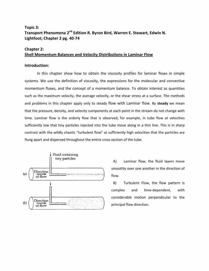
time. Laminar flow is the orderly flow that is observed, for example, in tube flow at velocities
sufficiently low that tiny particles injected into the tube move along in a thin line. This is in sharp
contrast with the wildly chaotic "turbulent flow" at sufficiently high velocities that the particles are
flung apart and dispersed throughout the entire cross section of the tube.
A) Laminar flow, the fluid layers move
smoothly over one another in the direction of
flow.
B) Turbulent Flow, the flow pattern is
complex and time‐dependent, with
considerable motion perpendicular to the
principal flow direction.

2. 1 SHELL MOMENTUM BALANCES AND BOUNDARY CONDITIONS Momentum balance for steady flow:
0
• This statement has a relation with the law of conservation of momentum. In the momentum
balance we need the expressions for the convective momentum fluxes given in Table 1.7‐1 and
the molecular momentum fluxes given in Table 1.2‐1. Is important that the molecular
momentum flux includes both the pressure and the viscous contributions.
• The momentum balance is applied only to systems in which there is just one velocity
component in this chapter, but it can be applied to system in which has more than one velocity
component, which depends on only one spatial variable, also the flow must be rectilinear.
The steps for setting up and solving viscous problems are:
1. Identify the nonvanishing velocity component and the spatial variable on which it depends.
2. Apply the momentum balance over a thin shell perpendicular to the relevant spatial
variable.
3. Find the limit when the thickness of the shell approach zero and make use of the definition
of the first derivative to obtain the corresponding differential equation for the momentum
flux.
4. Then integrate this equation to get the momentum‐flux distribution.
5. Insert Newton's law of viscosity and obtain a differential equation for the velocity.
6. Integrate this equation to get the velocity distribution.
7. Use the velocity distribution to get other quantities, such as the maximum velocity, average
velocity, or force on solid surfaces.
• These steps mentioned some integration, several constants of integration appear, and these
are evaluated by using boundary conditions that is statements about the velocity or stress
at the boundaries of the system. The most commonly used boundary conditions are as
follows:
A. At solid‐fluid interfaces the fluid velocity equals the velocity with which the solid
surface is moving. This statement is applied to both the tangential and the normal
component of the velocity vector. The equality of the tangential components is referred
to as the "no‐slip condition”.
B. At liquid‐liquid interfacial plane of constant x, the tangential velocity components Vy
and Vz are continuous through the interface (the "no‐slip condition") as are also the
molecular stress‐tensor components p + �xx, �xy and �xz.
C. At a liquid‐gas interfacial plane of constant x, the stress‐tensor components �xy and �xz
are taken to be zero, provided that the gas‐side velocity gradient is not too large. This is
logical, since the viscosities of gases are much less than those of liquids.
• In all of these boundary conditions it is supposed that there is no material passing through
the interface that is, there is no adsorption, absorption, dissolution, evaporation, melting, or
chemical reaction at the surface between the two phases.
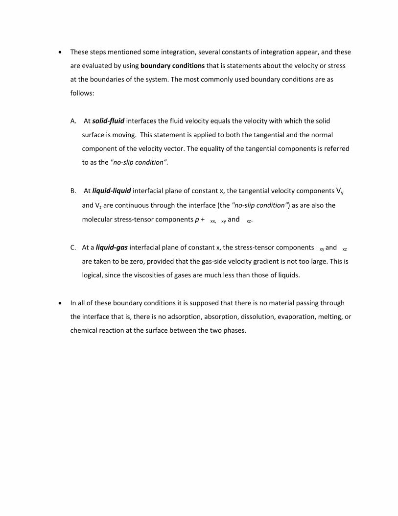
2.2 FLOW OF A FALLING FILM
• This example show a flow of a liquid an inclined flat plate of length L and width W, as shown
in the Figure. We consider the viscosity and density of the fluid to be constant. A complete
description of the liquid flow is difficult because of the disturbances at the edges of the
system (z = 0, z = L, y = 0, y = W).
• A description can often be obtained by neglecting such disturbances, particularly if W and L
are large compared to the film thickness δ.
• For small flow rates we expect that the viscous forces will prevent continued acceleration of
the liquid down the wall, so that V, will become independent of z in a short distance down
the plate.
• As a result it seems reasonable to postulate that Vz = Vz(x), Vx, = 0 and Vy = 0 and further that
p = p(x). The nonvanishing components of � are then �xz = �zx, = ‐μ (dVz/dx).
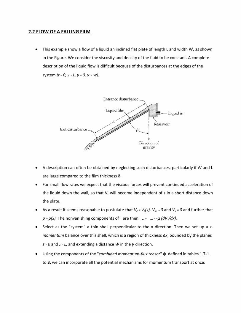
• Select as the "system" a thin shell perpendicular to the x direction. Then we set up a z‐
momentum balance over this shell, which is a region of thickness Δx, bounded by the planes
z = 0 and z = L, and extending a distance W in the y direction.
• Using the components of the "combined momentum‐flux tensor" φ defined in tables 1.7‐1 to 3, we can incorporate all the potential mechanisms for momentum transport at once:

• Using the quantities φxz and φzz we account for the z‐momentum transport by all mechanisms, convective and molecular.
• The "in" and "out" directions in the direction of the positive x‐ and z‐axes (in this problem these happen to coincide with the directions of z‐momentum transport). When these terms are substituted into the z‐momentum balance, we get:
LW(φxz�x ‐ φxz�x+Δx) + W Δx(φzz�z=0 ‐ φzz�z=L) + (LWΔX)(ρgcosβ) = 0
In this figure Δx is the thickness over which a z‐momentum balance is made. Arrows show
the momentum fluxes related with the surfaces of the shell. Since Vx and Vy are both zero,
ρVyVz and ρVyVz are zero. Vy does not depend on y and z, �yz = 0 and �zz = 0. Also the dashed‐
underlined fluxes do not need to be considered. Both p and ρVzVz are the same at z = 0 and z
= L, and as a result do not appear in the balance of z‐momentum.
Rate of z‐momentum in across surface at z=0 (W Δx)φzz /z=0
Rate of z‐momentum out across surface at z=L (W Δx)φzz /z=L
Rate of z‐momentum in across surface at x (LW)( φxz) /x
Rate of z‐momentum out across surface x + Δx (LW)( φxz) /x+Δx
Gravity force acting on fluid in the z direction (LW Δx)(ρgcosβ)
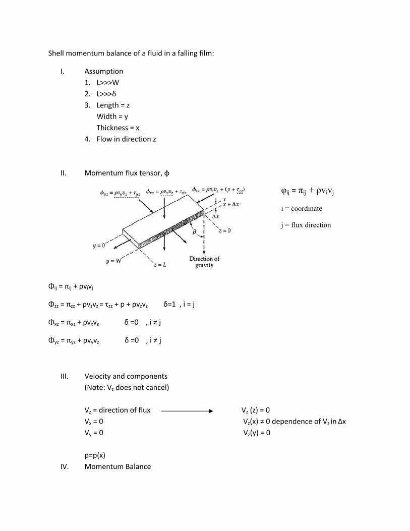
Shell momentum balance of a fluid in a falling film:
I. Assumption 1. L>>>W 2. L>>>δ 3. Length = z
Width = y Thickness = x
4. Flow in direction z
II. Momentum flux tensor, φ
Φij = πij + ρvivj
Φzz = πzz + ρvzvz = τzz + p + ρvzvz δ=1 , i = j
Φxz = πxz + ρvxvz δ =0 , i ≠ j
Φyz = πyz + ρvyvz δ =0 , i ≠ j
III. Velocity and components (Note: Vz does not cancel) Vz = direction of flux Vz (z) = 0 Vx = 0 Vz(x) ≠ 0 dependence of Vz in Δx Vy = 0 Vz(y) = 0 p=p(x)
IV. Momentum Balance
φij = πij + ρvivj
i = coordinate
j = flux direction
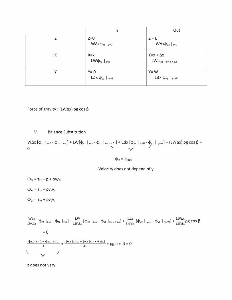
In Out
Z Z=0 WΔxφzz |z=0
Z = L WΔxφzz |z=L
X X=x LWφxz |x=x
X=x + Δx LWφxz |x= x + Δx
Y Y= 0
L x φyz | y=0
Y= W L x φyz | y=W
Force of gravity : (LWΔx) ρg cos β
V. Balance Substitution
WΔx [φzz |z=0 ‐ φzz |z=L] + LW[φxz |x=x ‐ φxz |x= x + Δx] + L x [φyz | y=0 ‐ φyz | y=W] + (LWΔx) ρg cos β = 0
φin = φout
Velocity does not depend of y
Φzz = τzz + p + ρvzvz
Φxz = τxz + ρvxvz
Φyz = τyz + ρvyvz
WΔ [φzz |z=0 ‐ φzz |z=L] +
LW [φxz |x=x ‐ φxz |x= x + Δx] +
L [φyz | y=0 ‐ φyz | y=W] +
LWΔ ρg cos β
= 0
φ | φ | L +
φ | φ | Δ + ρg cos β = 0
z does not vary
lim∆ φ | φ | Δ
= ‐ ρg cos β
ρg cos β
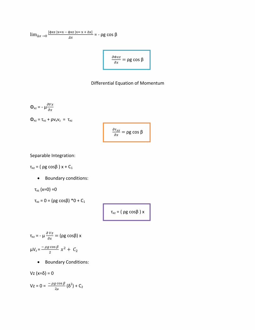
Differential Equation of Momentum
Φxz = ‐ µ
Φxz = τxz + ρvxvz = τxz
ρg cos β
Separable Integration:
τxz = ( ρg cosβ ) x + C1
• Boundary conditions:
τxz (x=0) =0
τxz = 0 = (ρg cosβ) *0 + C1
τxz = ( ρg cosβ ) x
τxz = ‐ µ (ρg cosβ) x
µVz =
• Boundary Conditions:
Vz (x=δ) = 0
Vz = 0 =
µ (δ2) + C2
C2 =
µ (δ2)
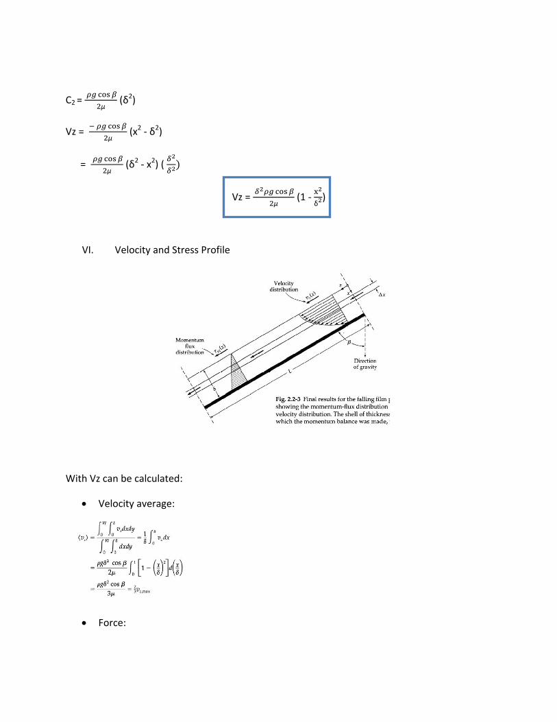
Vz =
µ (x2 ‐ δ2)
=
µ (δ2 ‐ x2) (
Vz =
µ (1 ‐
δ)
VI. Velocity and Stress Profile
With Vz can be calculated:
• Velocity average:
• Force:

• Thickness:
• Mass rate:
• Maximum Velocity:
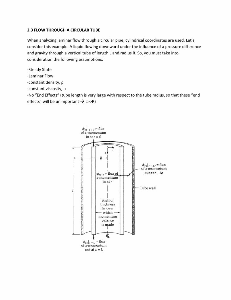
2.3 FLOW THROUGH A CIRCULAR TUBE
When analyzing laminar flow through a circular pipe, cylindrical coordinates are used. Let’s consider this example. A liquid flowing downward under the influence of a pressure difference and gravity through a vertical tube of length L and radius R. So, you must take into consideration the following assumptions:
‐Steady State ‐Laminar Flow ‐constant density, ρ ‐constant viscosity, µ ‐No “End Effects” (tube length is very large with respect to the tube radius, so that these “end effects” will be unimportant L>>R)

Postulates: (Look at the coordinate system in the diagram)
• Vz= Vz(r)
• Vr=0
• Vθ=0
• Vz(z)=0
• Vz(θ)=0
• Vz(r) 0
• p=p(z)
From these terms when you go to Table B.1/Appendix B on your BSL book (pg. 844) the nonvanishing components of are τrz and τzr, because of the postulates shown above.
When making a momentum balance, you first need to look at where the momentum is generated when the fluid is flowing downward. Momentum is generated in z and r directions as seen in the coordinate system below and we can put this coordinate system in half of our cylinder to analyze it.
The quantities of and account for the momentum transport by all possible mechanisms, convective and molecular. As for the values of those momentums, and you’re not sure how to evaluate them, Table 1.2‐1 (pg. 17), Table 1.7‐1(pg. 35) and equation 1.7‐2 (pg.36) can help. Remember you will eventually need these values when making shell balances. Therefore if we have,

Then,
Ok, so back to our momentum balance. We select our system as a cylindrial shell of thickness ∆ and length L. We evaluate the momentum in and out of this shell and we can then list the contributions:
Directions In Out
R r=r 2 | ∆ 2 | ∆
Z z=0 2 ∆ | z=L 2 ∆ |
Θ No rate of momentum in this
direction No rate of momentum in this
direction
Gravity force acting in z direction on cylindrical shell 2 ∆
* Note that those “in” and “out” are in the positive direction of the r and z‐axes.
We now make our momentum balance based on equation 2.1‐1 (pg. 41) from your BSL book:
2 | | ∆ 2 ∆ | | 2 ∆ 0
We then divide this equation by 2 ∆ to get:
| | ∆
∆| |
0
The same as,
| ∆ |∆
| |
By taking the limit of the equation on the left side when r 0, we get:
lim| ∆ |
∆| |

And by definition,
lim| ∆ |
∆
Therefore,
| |
Now we evaluate the components and with the values in Appendix B.1 :
2
(*Remember: Vr=0)
By substituting these values in and :
2
We now have the following simplifications:
1) Because we have Vz=Vz(r), the term will be the same at both ends of the tube. | |
2) Because we have Vz=Vz(r), the term 2 will be the same at both ends of the
tube.
2 | 2 |
So now our equations turns into:
0
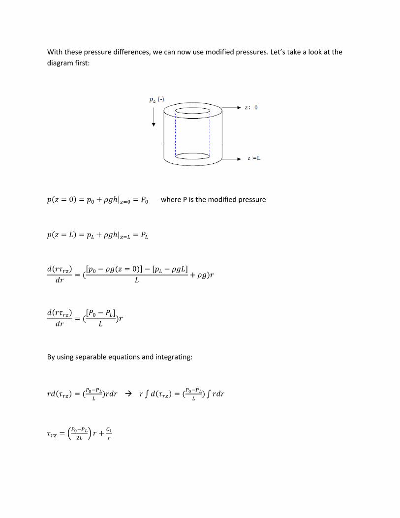
With these pressure differences, we can now use modified pressures. Let’s take a look at the diagram first:
0 | where P is the modified pressure
|
0
By using separable equations and integrating:

To look for the value of constant C1, we use certain boundary conditions to simplify our problem. Let’s look at the following diagram, where we can watch the velocity profile:
Boundary Condition 1:
• When r=0, =0
Therefore, C1=0 and by substituting with Newton’s Law of Viscosity (obtained from Apendix
B.2) we obtain:
2
Integrating this first order differential equation we obtain:
4
This new constant C2 is evaluated from the boundary condition
B.C. 2: at r=R, vz = 0
Then, from this C2 is found to be: 4⁄ . Hence, the velocity distribution is:
4 1
We see that the velocity distribution for laminar, incompressible flow of a Newtonian fluid in a long tube is parabolic.
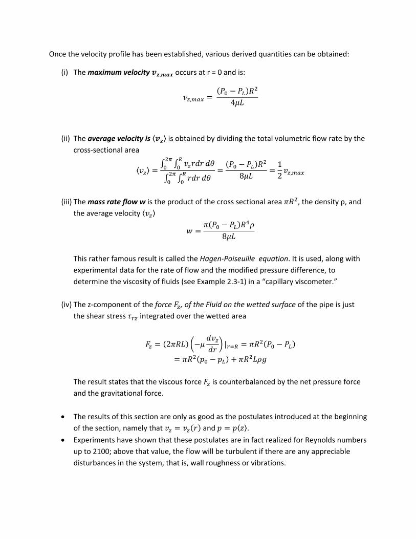
Once the velocity profile has been established, various derived quantities can be obtained:
(i) The maximum velocity , occurs at r = 0 and is:
, 4
(ii) The average velocity is is obtained by dividing the total volumetric flow rate by the cross‐sectional area
812 ,
(iii) The mass rate flow w is the product of the cross sectional area , the density ρ, and
the average velocity
8
This rather famous result is called the Hagen‐Poiseuille equation. It is used, along with experimental data for the rate of flow and the modified pressure difference, to determine the viscosity of fluids (see Example 2.3‐1) in a “capillary viscometer.”
(iv) The z‐component of the force , of the Fluid on the wetted surface of the pipe is just the shear stress integrated over the wetted area
2 |
The result states that the viscous force is counterbalanced by the net pressure force and the gravitational force.
• The results of this section are only as good as the postulates introduced at the beginning of the section, namely that and .
• Experiments have shown that these postulates are in fact realized for Reynolds numbers up to 2100; above that value, the flow will be turbulent if there are any appreciable disturbances in the system, that is, wall roughness or vibrations.
• For circular tubes the Reynolds number is defined by ⁄ , where D=2R is the tube diameter.
We now summarize all the assumptions that were made in obtaining the Hagen‐Poiseuille equation.
(a) The flow is laminar (Re < 2100) (b) Density is constant (“incompressible flow”) (c) The flow is “steady” (i.e. does not change with time) (d) The fluid is Newtonian (e) End effects are neglected. Actually an “entrance length,” after the tube entrance of
the order of Le=0.035D Re, is needed for the buildup of the parabolic profiles. If the section of the pipe of interest includes the entrance region, a correction must be applied. The fractional correction in the pressure difference or mass rate of flow never exceeds Le/L if L>Le.
(f) The fluid behaves as a continuum, this assumption is valid, except for very dilute gases or very narrow capillary tubes, in which the molecular mean free path is comparable to the tube diameter (the “slip flow region”) or much greater than the tube diameter (the “Kundsen flow” or “free molecule flow” regime).
(g) There is no slip at the wall, so that B.C. 2 is valid; this is an excellent assumption fot pure fluids under the conditions assumed in (f).
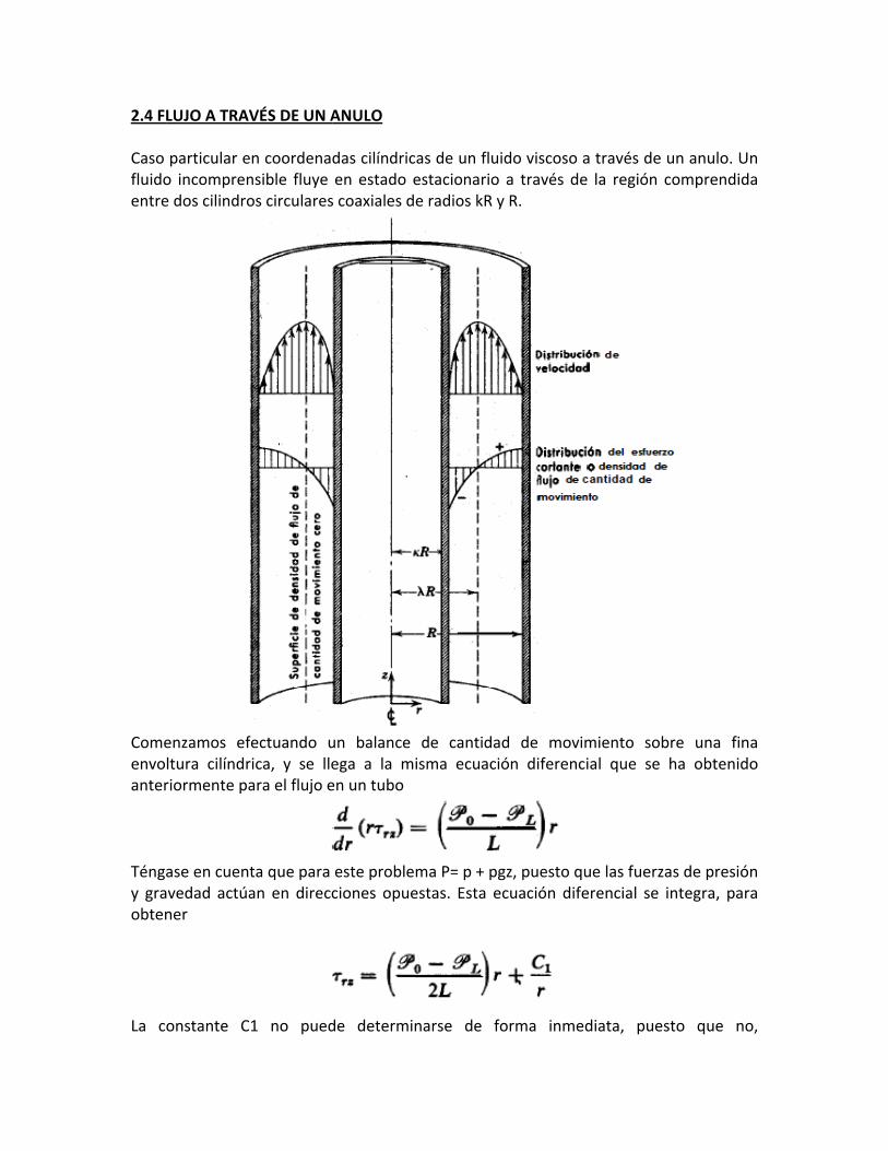
2.4 F Caso fluidoentre
Comeenvoanter
Téngay graobten
La c
LUJO A TRAV
particular eo incomprene dos cilindro
enzamos efltura cilíndrriormente pa
ase en cuenavedad actúaner
onstante C
VÉS DE UN A
en coordenansible fluye os circulares
fectuando urica, y se lleara el flujo e
ta que para an en direcc
1 no pued
ANULO
das cilíndricen estado es coaxiales d
un balance ega a la men un tubo
este probleciones opue
de determin
as de un fluestacionarioe radios kR y
de cantidaisma ecuaci
ma P= p + pgestas. Esta e
narse de f
ido viscoso o a través dey R.
ad de moviión diferenc
gz, puesto qecuación dif
forma inme
a través de e la región
imiento sobcial que se
que las fuerzerencial se
ediata, pues
un anulo. Ucomprendid
bre una finha obtenid
as de presióintegra, par
sto que no
n da
na do
ón ra
o,

dispoen niexistir=λR,
Tenieque l
Nótehabe
la ecuecuac
Integ
Ahorasiguie
Substecuac
Se re
onemos de inguna de lair un máximo, para el cu
endo esto ena ecuación a
se que λ esr substituido
uación anterción diferen
grando con r
a pueden eventes condic
tituyendo esciones simul
suelve y se e
nformación as dos supero de la curvaual la densid
n cuenta, puanterior se t
todavía uno C1 por λ es
rior la ley decial:
especto a r:
valuarse las dciones límite
CL 1:
CL 2:
stas condicioltáneas
encuentra
acerca de larficies r=kR oa de velociddad de flujo
uede substitransforma e
a constantes que conoc
e la viscosida
dos constane:
p
p
ones límites
a densidad do r=R. Lo mad en un cieo de cantid
tuirse C1 poen
e de integracemos el sign
ad de Newto
tes de integ
ara r=kR
para r=R
en la ecuaci
de flujo, de ás que podeerto plano (had de movi
or
ción desconnificado físic
on
ración λ y C2
vz
vz
ón anterior
cantidad deemos decir hasta ahora imiento ha
ocida. La úno de λ. Subs
se
2, utilizando
z=0
z=0
se obtienen
e movimientes que ha ddesconocidode ser cero
, con l
nica razón dstituyendo e
e obtiene est
o las dos
n estas dos
to de o) o.
lo
de en
ta
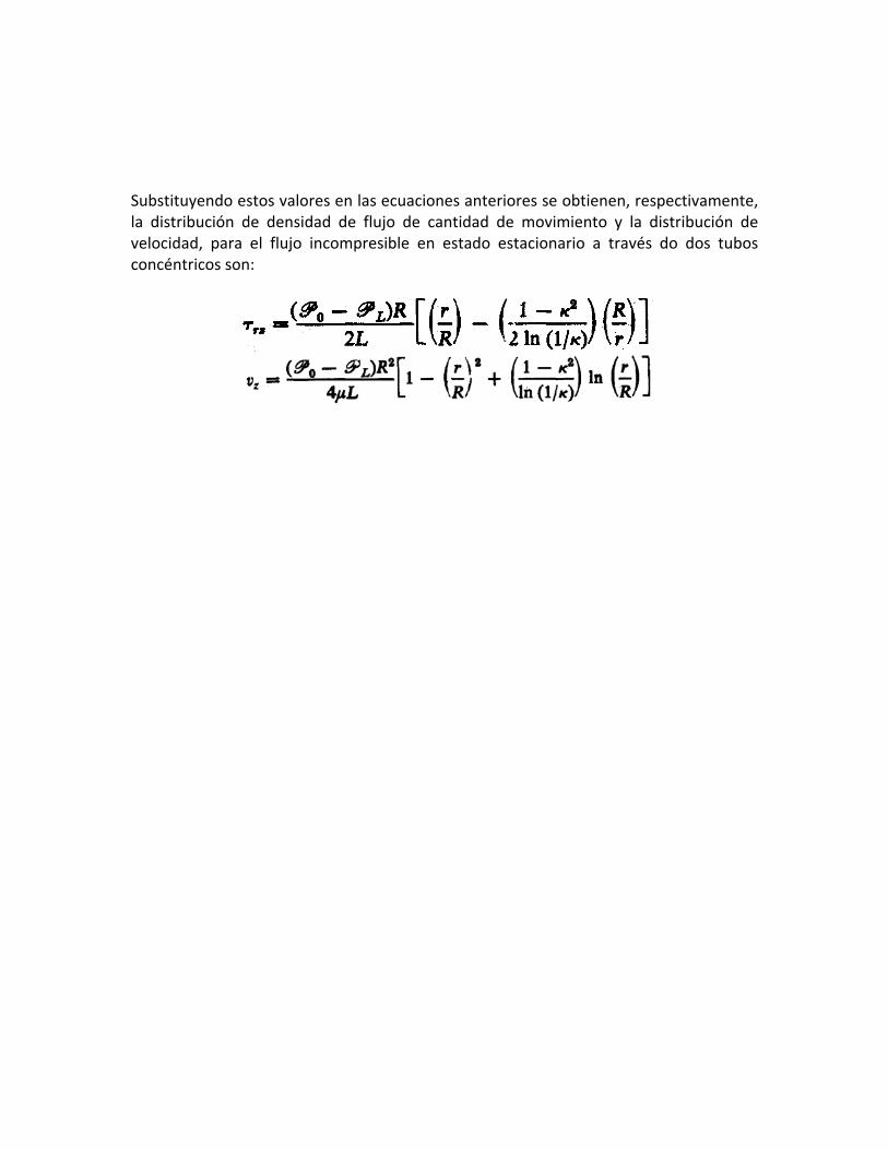
Substla disvelocconcé
tituyendo esstribución dcidad, para éntricos son
stos valores de densidad el flujo inco:
en las ecuade flujo deompresible
ciones antere cantidad den estado
riores se obtde movimieestacionario
tienen, respento y la diso a través d
pectivamentestribución ddo dos tubo
e, de os
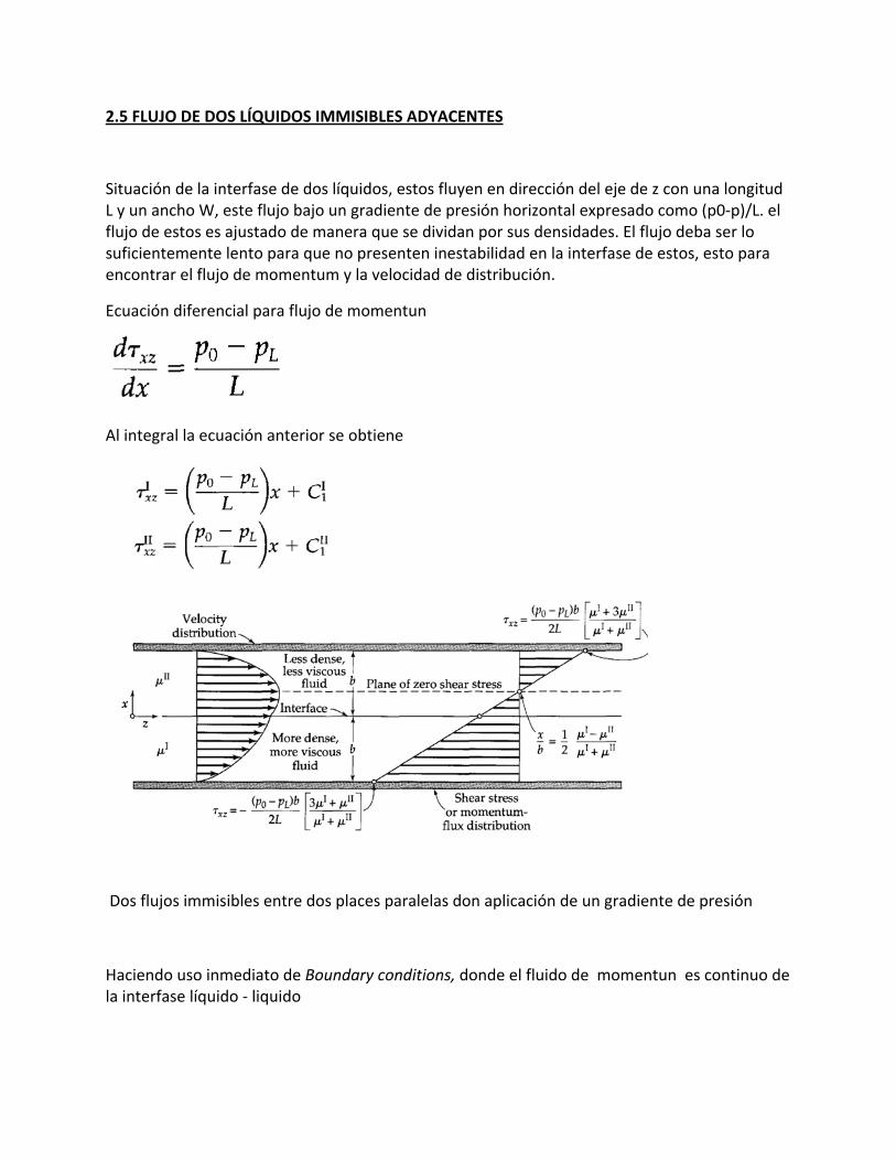
2.5 FLUJO DE DOS LÍQUIDOS IMMISIBLES ADYACENTES
Situación de la interfase de dos líquidos, estos fluyen en dirección del eje de z con una longitud L y un ancho W, este flujo bajo un gradiente de presión horizontal expresado como (p0‐p)/L. el flujo de estos es ajustado de manera que se dividan por sus densidades. El flujo deba ser lo suficientemente lento para que no presenten inestabilidad en la interfase de estos, esto para encontrar el flujo de momentum y la velocidad de distribución.
Ecuación diferencial para flujo de momentun
Al integral la ecuación anterior se obtiene
Dos flujos immisibles entre dos places paralelas don aplicación de un gradiente de presión
Haciendo uso inmediato de Boundary conditions, donde el fluido de momentun es continuo de la interfase líquido ‐ liquido

B.C. 1: at x = 0, =
Las y serán la constantes de la integra, estas igual a
La sustituir la leu de viscosidad de newton’s, en Fig. 2.5‐2 y 2.5‐3 obtenemos
Estas se pueden entegrar para obtener
Las tres constantes de integracion se pueden determinar siguiendo No‐slip B.C. B.C. 2: atx = 0, vIz = VII
z
B.C. 3: atx = ‐b, v = 0 B.C. 4: atx = +b, v = 0
Cuando estas tres condiciones son aplicadas, conseguimos tres ecuaciones simultáneas para las constantes de la integración:
De estas tres ecuaciones conseguimos

Los resultados del flujo de momentun y perfil de velocidad son
Si ambas viscosidades son iguales, después de la distribución de la velocidad es parabólica
La velocidad media en cada capa puede ser obtenida y resultaría
Las distribuciones de la velocidad dadas arriba, se podría obtener la velocidad máxima, la velocidad en la interfase, el plano cero del estrés cortante, y la fricción en las paredes.
Anteriormente se han solucionado problemas de flujos viscosos. Se han tratado solo componentes rectilíneos con un componente de velocidad. El flujo alrededor de una esfera aplica dos componentes nonvanishing de la velocidad, vr y vø no se puede explicar convenientemente por las técnicas explicadas al principio de este capítulo. Una breve discusión del flujo alrededor de una esfera se determina aquí debido a la importancia del flujo alrededor de objetos. En el capítulo 4 se demuestra cómo obtener las distribuciones de la velocidad y de presión. Aquí se muestra los resultados y como pueden ser utilizados para ciertas derivaciones posteriormente. Aquí como en el capítulo 4, se trabaja con el arrastre del flujo. (este en un flujo lento)
Consideramos aquí el flujo de un líquido incompresible sobre una esfera sólida del radio R y del
diámetro D según las indicaciones de fig. 2.6‐1. El líquido, con la densidad p y la viscosidad

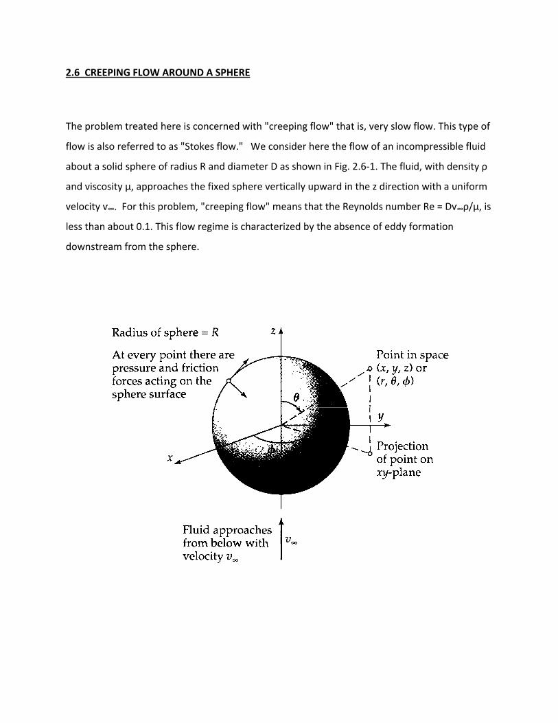
2.6 CREEPING FLOW AROUND A SPHERE
The problem treated here is concerned with "creeping flow" that is, very slow flow. This type of
flow is also referred to as "Stokes flow." We consider here the flow of an incompressible fluid
about a solid sphere of radius R and diameter D as shown in Fig. 2.6‐1. The fluid, with density ρ
and viscosity μ, approaches the fixed sphere vertically upward in the z direction with a uniform
velocity ѵ∞. For this problem, "creeping flow" means that the Reynolds number Re = Dѵ∞ρ/μ, is
less than about 0.1. This flow regime is characterized by the absence of eddy formation
downstream from the sphere.
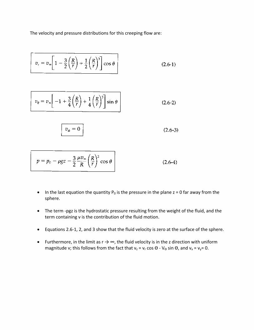
The velocity and pressure distributions for this creeping flow are:
• In the last equation the quantity P0 is the pressure in the plane z = 0 far away from the sphere.
• The term ‐pgz is the hydrostatic pressure resulting from the weight of the fluid, and the term containing v is the contribution of the fluid motion.
• Equations 2.6‐1, 2, and 3 show that the fluid velocity is zero at the surface of the sphere.
• Furthermore, in the limit as r → ∞, the fluid velocity is in the z direction with uniform magnitude v; this follows from the fact that vz = vr cos Ѳ ‐ VѲ sin Ѳ, and vx = vy= 0.
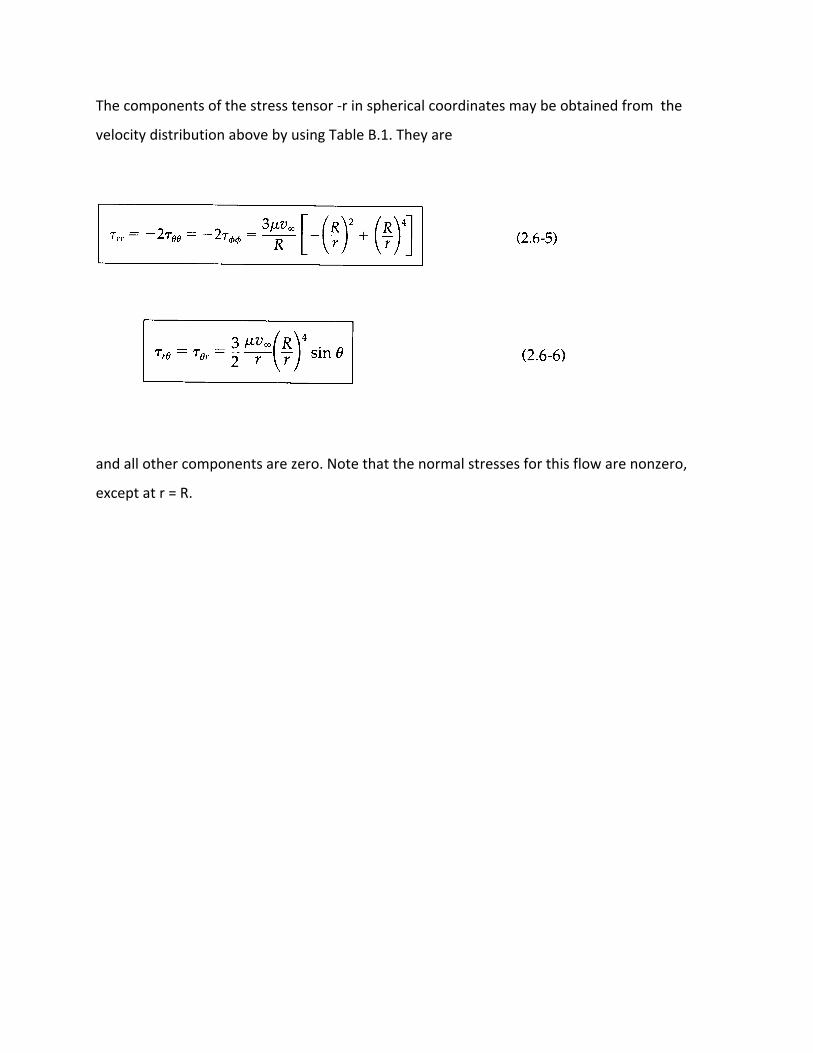
The components of the stress tensor ‐r in spherical coordinates may be obtained from the
velocity distribution above by using Table B.1. They are
and all other components are zero. Note that the normal stresses for this flow are nonzero,
except at r = R.
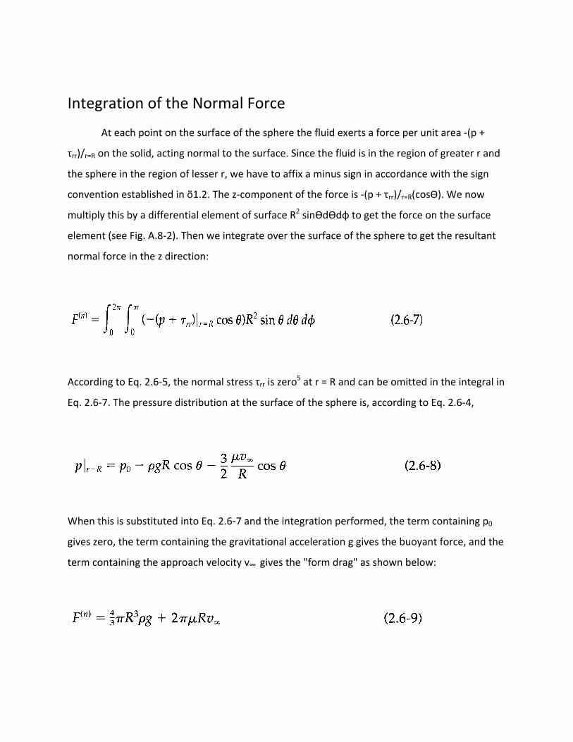
Integration of the Normal Force
At each point on the surface of the sphere the fluid exerts a force per unit area ‐(p +
τrr)/r=R on the solid, acting normal to the surface. Since the fluid is in the region of greater r and
the sphere in the region of lesser r, we have to affix a minus sign in accordance with the sign
convention established in õ1.2. The z‐component of the force is ‐(p + τrr)/r=R(cosѲ). We now
multiply this by a differential element of surface R2 sinѲdѲdφ to get the force on the surface
element (see Fig. A.8‐2). Then we integrate over the surface of the sphere to get the resultant
normal force in the z direction:
According to Eq. 2.6‐5, the normal stress τrr is zero5 at r = R and can be omitted in the integral in
Eq. 2.6‐7. The pressure distribution at the surface of the sphere is, according to Eq. 2.6‐4,
When this is substituted into Eq. 2.6‐7 and the integration performed, the term containing p0
gives zero, the term containing the gravitational acceleration g gives the buoyant force, and the
term containing the approach velocity v∞ gives the "form drag" as shown below:
The buoyant force is the mass of displaced fluid (4/3 πR3ρ) times the gravitational acceleration
(g).
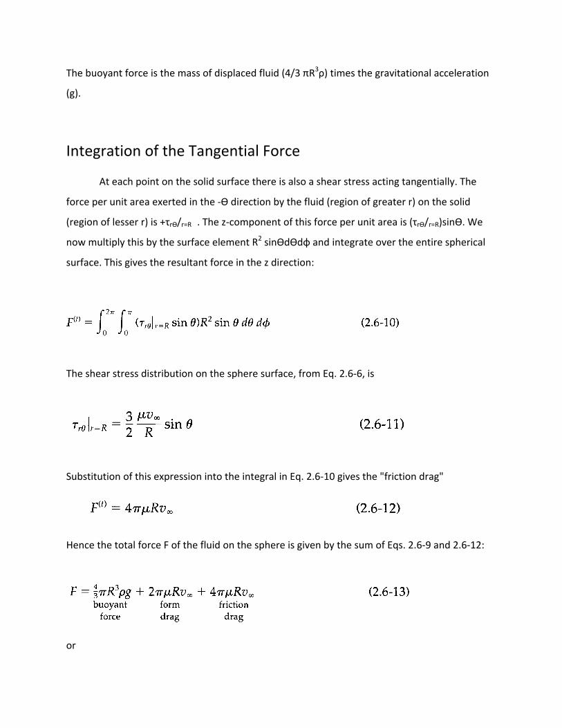
Integration of the Tangential Force
At each point on the solid surface there is also a shear stress acting tangentially. The
force per unit area exerted in the ‐Ѳ direction by the fluid (region of greater r) on the solid
(region of lesser r) is +τrѲ/r=R�. The z‐component of this force per unit area is (τrѲ/r=R)sinѲ. We
now multiply this by the surface element R2 sinѲdѲdφ and integrate over the entire spherical
surface. This gives the resultant force in the z direction:
The shear stress distribution on the sphere surface, from Eq. 2.6‐6, is
Substitution of this expression into the integral in Eq. 2.6‐10 gives the "friction drag"
Hence the total force F of the fluid on the sphere is given by the sum of Eqs. 2.6‐9 and 2.6‐12:
or
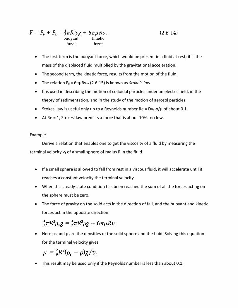
• The first term is the buoyant force, which would be present in a fluid at rest; it is the
mass of the displaced fluid multiplied by the gravitational acceleration.
• The second term, the kinetic force, results from the motion of the fluid.
• The relation Fk = 6πμRѵ∞ (2.6‐15) is known as Stoke’s law.
• It is used in describing the motion of colloidal particles under an electric field, in the
theory of sedimentation, and in the study of the motion of aerosol particles.
• Stokes' law is useful only up to a Reynolds number Re = Dv∞ρ/μ of about 0.1.
• At Re = 1, Stokes' law predicts a force that is about 10%.too low.
Example
Derive a relation that enables one to get the viscosity of a fluid by measuring the
terminal velocity ѵt of a small sphere of radius R in the fluid.
• If a small sphere is allowed to fall from rest in a viscous fluid, it will accelerate until it
reaches a constant velocity the terminal velocity.
• When this steady‐state condition has been reached the sum of all the forces acting on
the sphere must be zero.
• The force of gravity on the solid acts in the direction of fall, and the buoyant and kinetic
forces act in the opposite direction:
• Here ps and p are the densities of the solid sphere and the fluid. Solving this equation
for the terminal velocity gives
• This result may be used only if the Reynolds number is less than about 0.1.


