TwoTwo--scale Tone Management for scale Tone Management for Photographic LookPhotographic Look

Soonmin Bae, Sylvain Paris, and Frédo Durand

MIT CSAIL

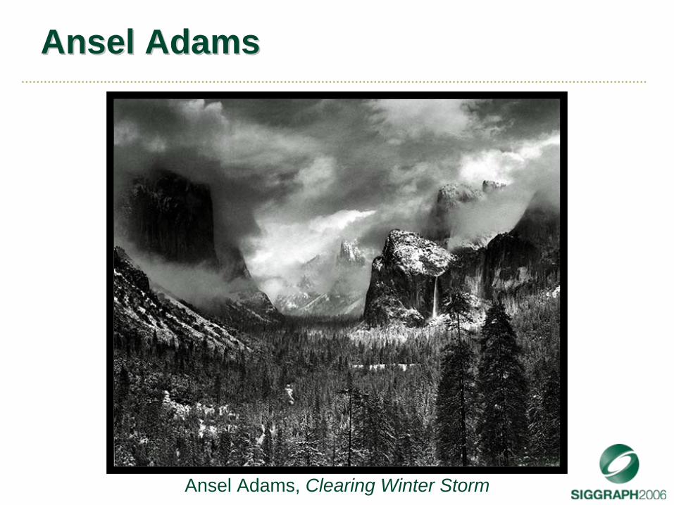
AnselAnsel AdamsAdams

Ansel Adams, Clearing Winter Storm

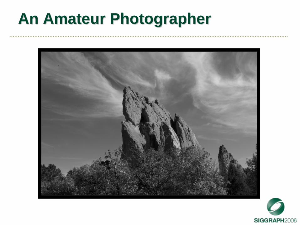
An Amateur PhotographerAn Amateur Photographer

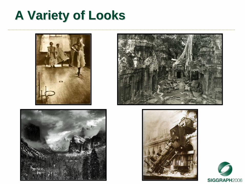
A Variety of LooksA Variety of Looks

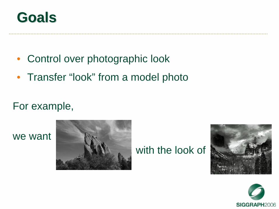
GoalsGoals

• Control over photographic look

• Transfer “look” from a model photo

For example,

we wantwith the look of

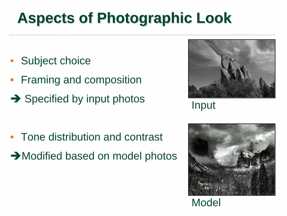
Aspects of Photographic LookAspects of Photographic Look

• Subject choice

• Framing and composition

Specified by input photos

• Tone distribution and contrast

Modified based on model photos

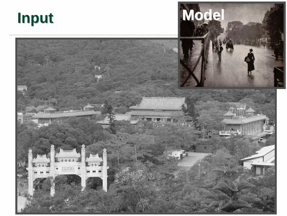
Input

Model

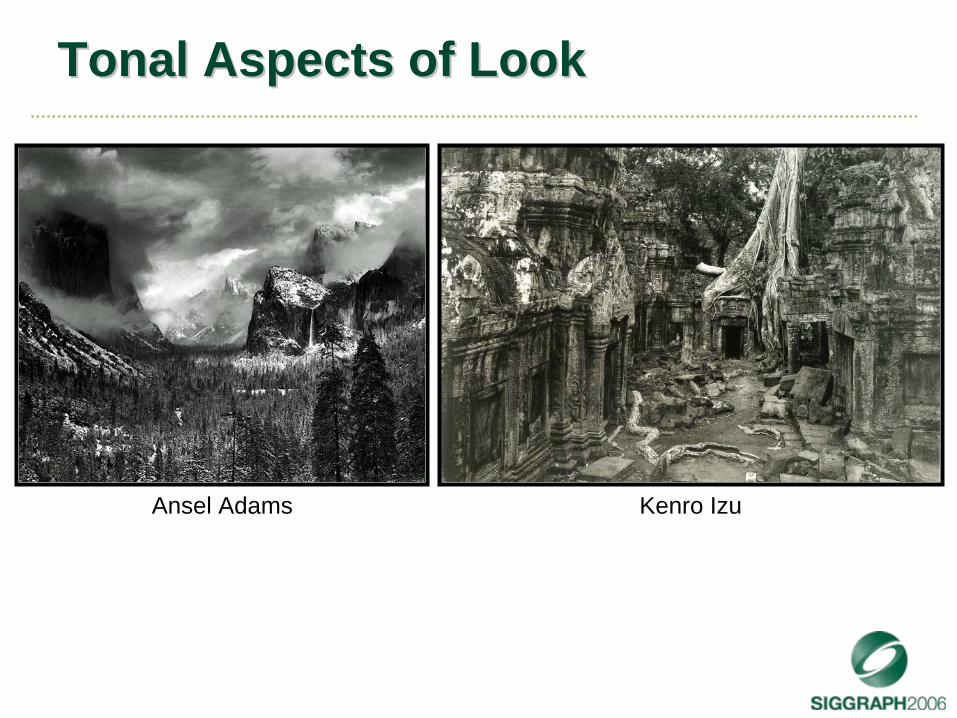
Tonal Aspects of LookTonal Aspects of Look

Ansel Adams Kenro Izu

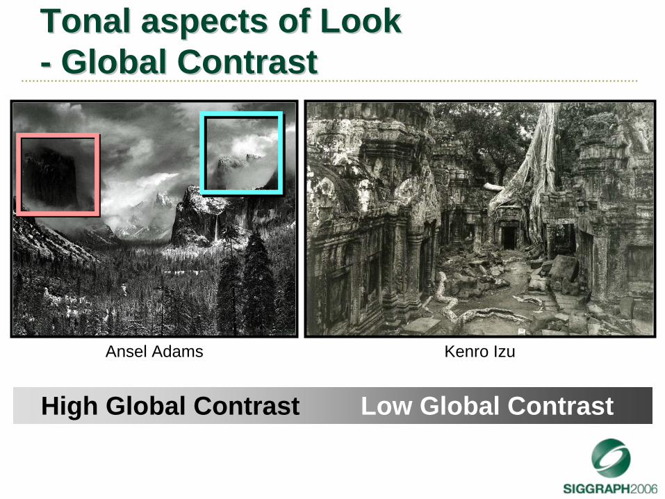
Tonal aspects of LookTonal aspects of Look -- Global ContrastGlobal Contrast

Ansel Adams Kenro Izu

High Global Contrast Low Global Contrast

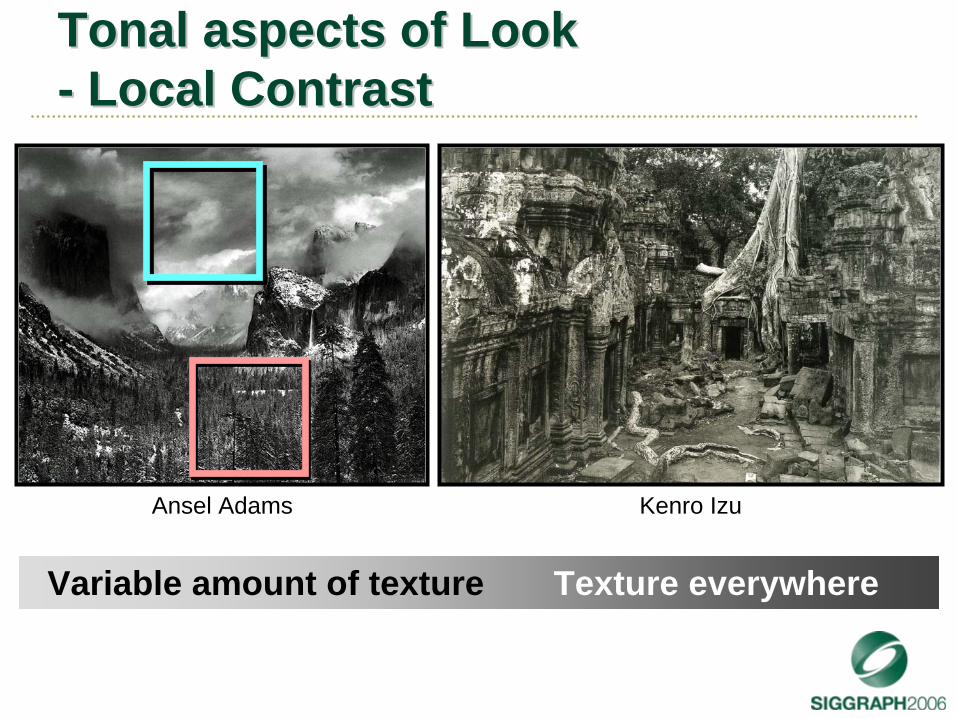
Tonal aspects of Look Tonal aspects of Look -- Local ContrastLocal Contrast

Variable amount of texture Texture everywhere

Ansel Adams Kenro Izu

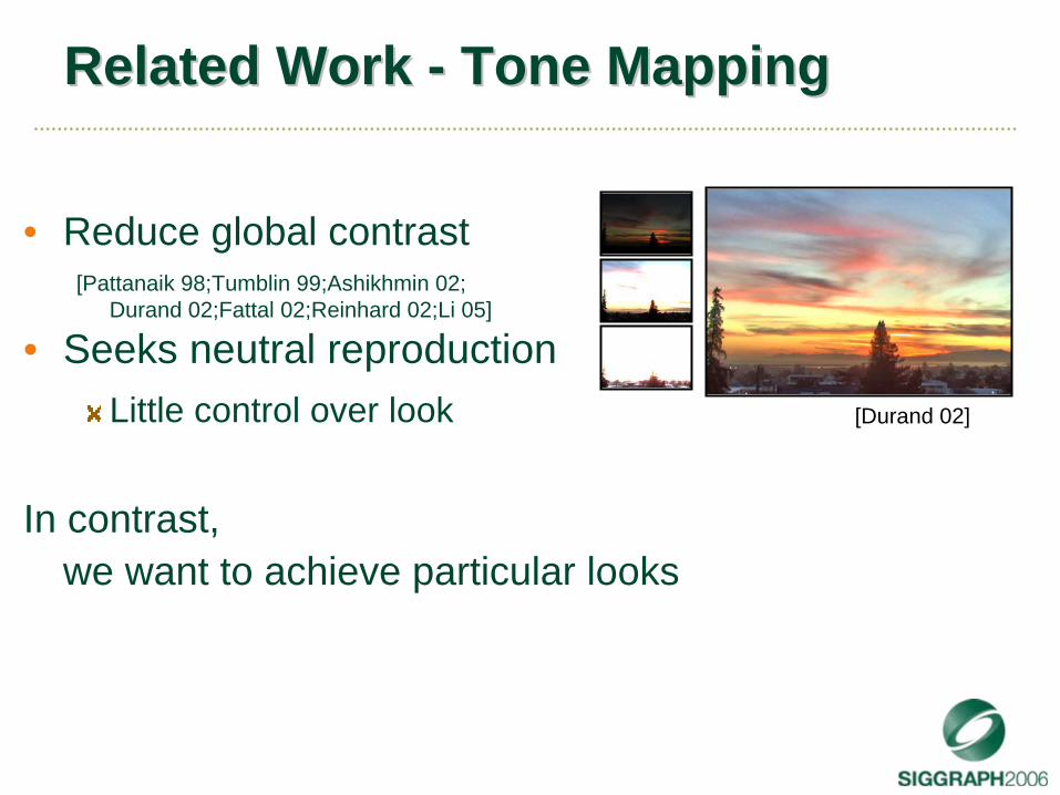
Related Work Related Work -- Tone MappingTone Mapping

• Reduce global contrast[Pattanaik 98;Tumblin 99;Ashikhmin 02;

Durand 02;Fattal 02;Reinhard 02;Li 05]

• Seeks neutral reproductionLittle control over look

In contrast, we want to achieve particular looks

[Durand 02]

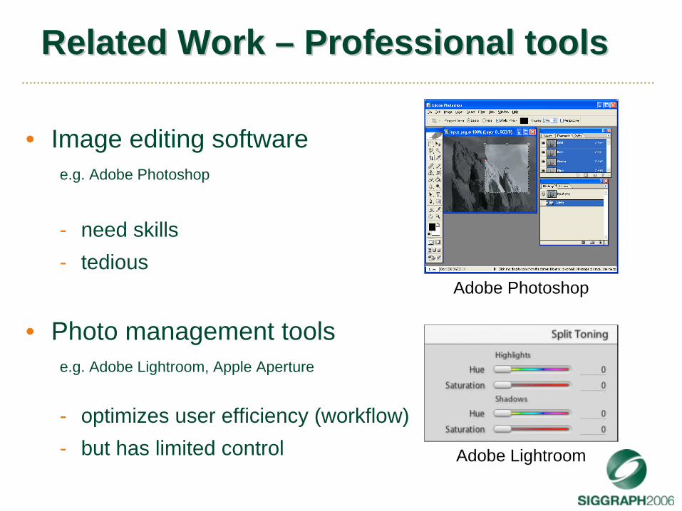
Related Work Related Work –– Professional toolsProfessional tools

• Image editing softwaree.g. Adobe Photoshop

- need skills - tedious

• Photo management toolse.g. Adobe Lightroom, Apple Aperture

- optimizes user efficiency (workflow)- but has limited control Adobe Lightroom

Adobe Photoshop

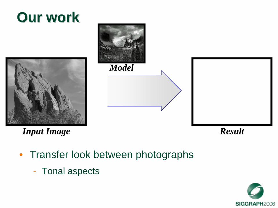
Our workOur work

Input Image Result

Model

• Transfer look between photographs- Tonal aspects

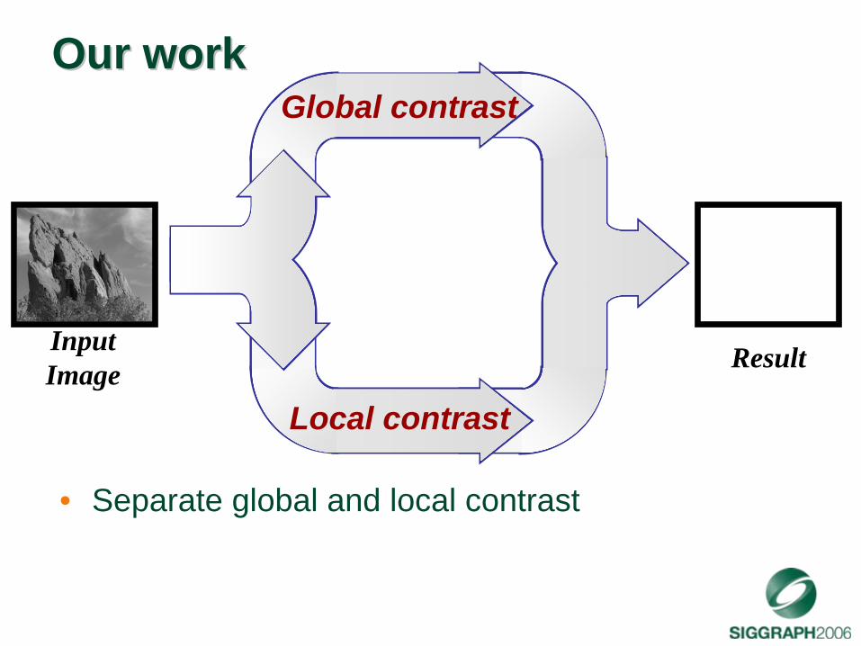
Our workOur work

Local contrast

Global contrast

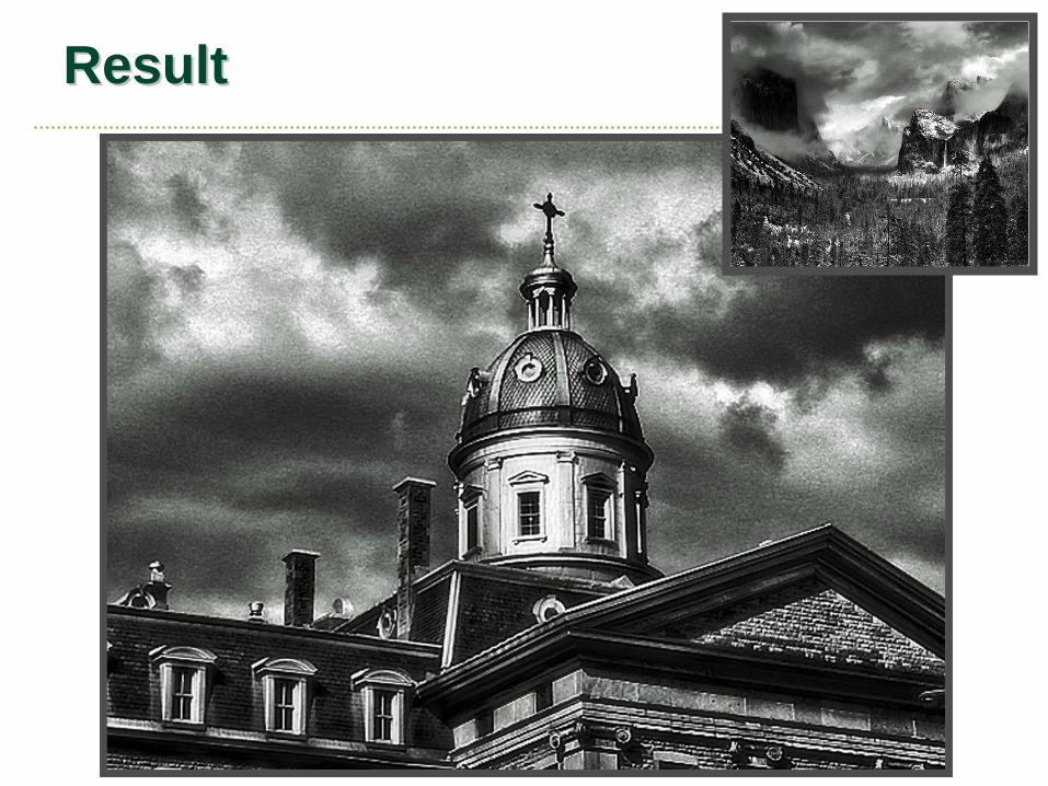
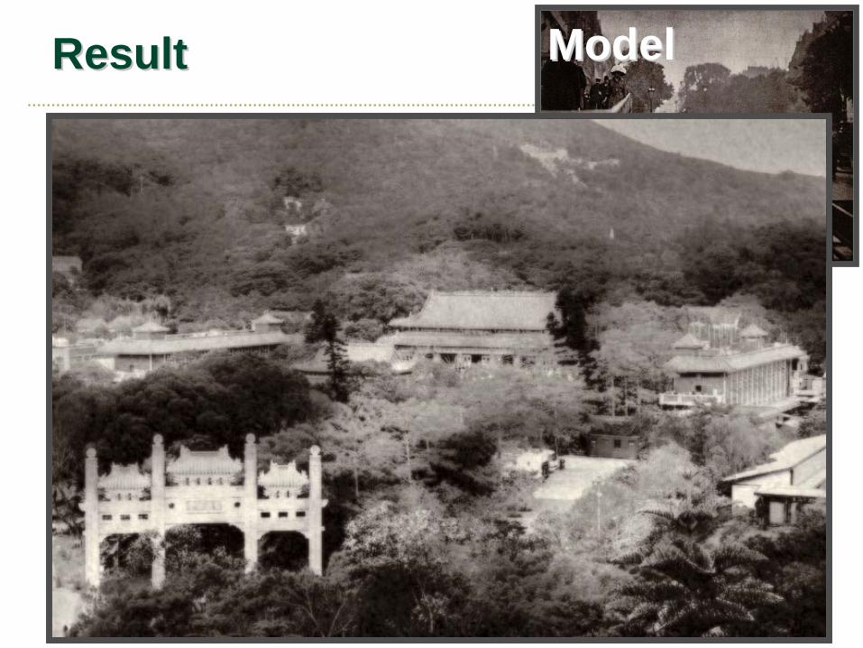
Result

• Separate global and local contrast

Input Image

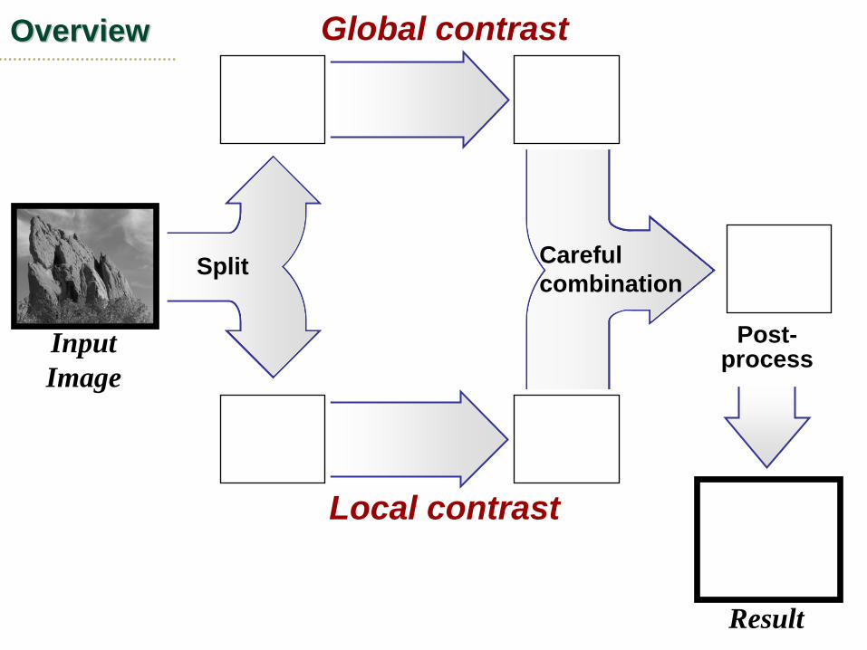
Split

Local contrast

Global contrast

Input Image

Result

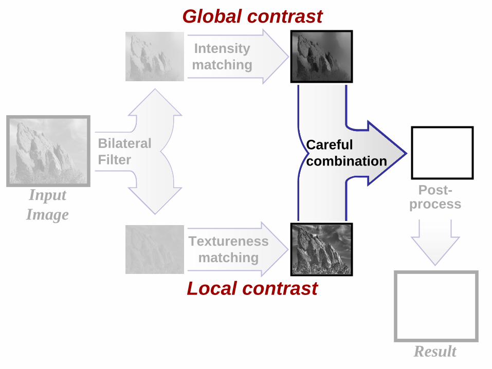
Careful combination

Post- process

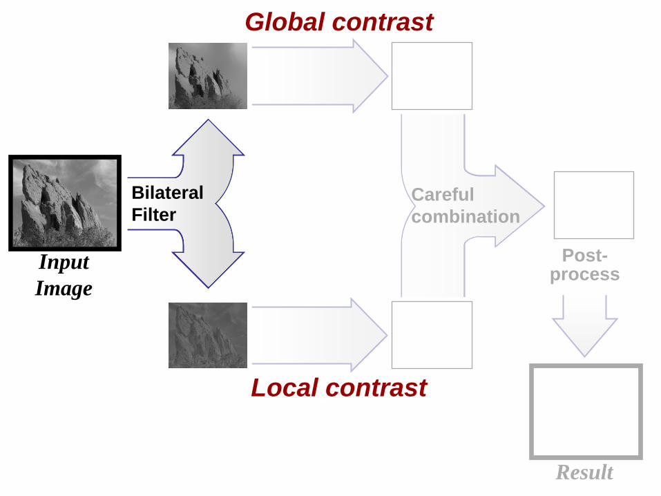
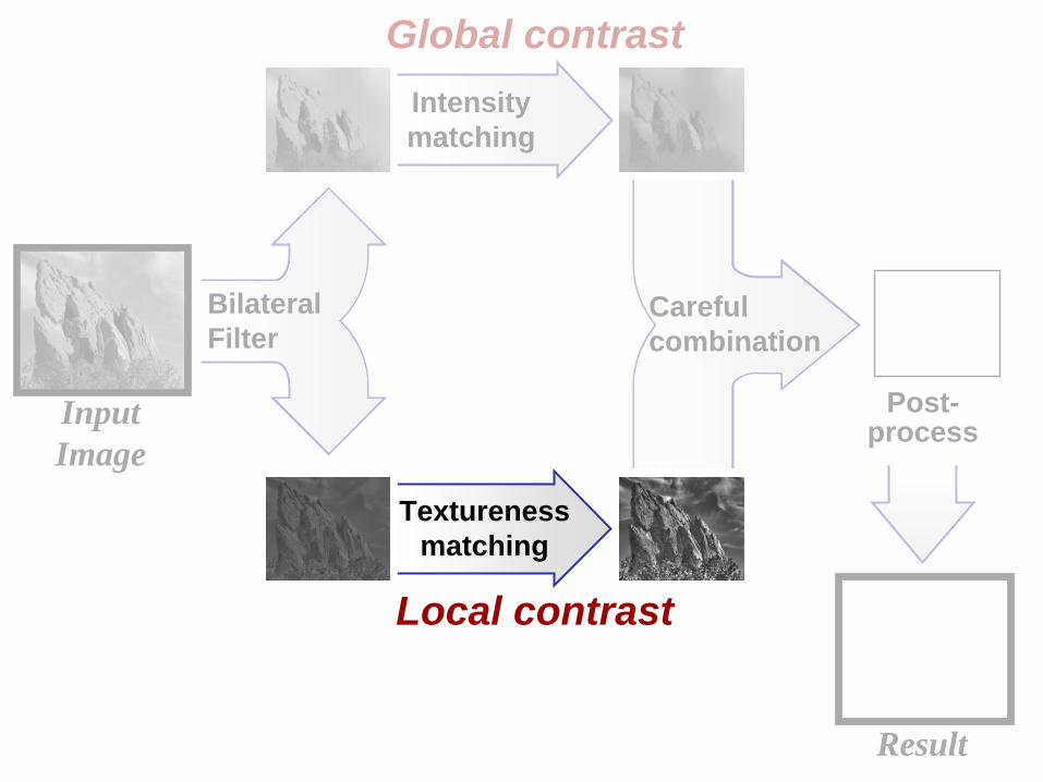
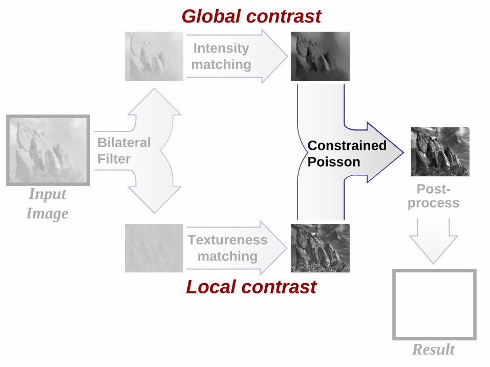
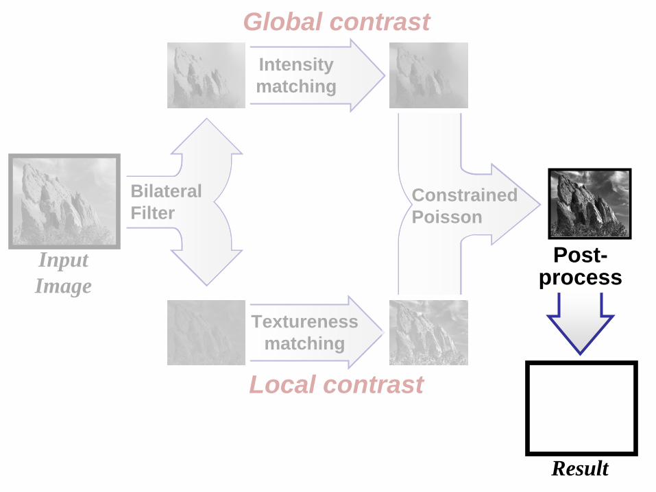
OverviewOverview

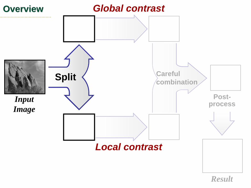
Split

Global contrast

Input Image

Result

Careful combination

Post- process

OverviewOverview

Local contrast

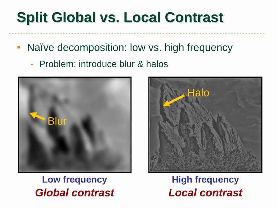
Split Global vs. Local ContrastSplit Global vs. Local Contrast

• Naïve decomposition: low vs. high frequency- Problem: introduce blur & halos

Low frequency High frequency

Halo

Blur

Global contrast Local contrast

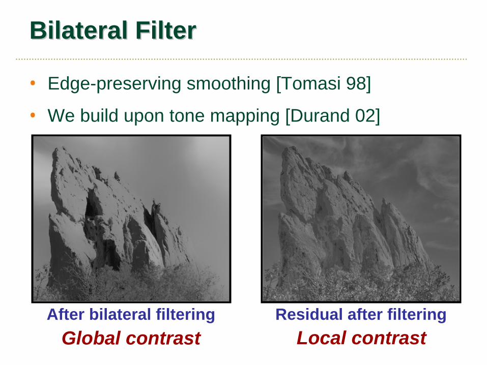
Bilateral FilterBilateral Filter

• Edge-preserving smoothing [Tomasi 98]

• We build upon tone mapping [Durand 02]

After bilateral filtering Residual after filteringGlobal contrast Local contrast

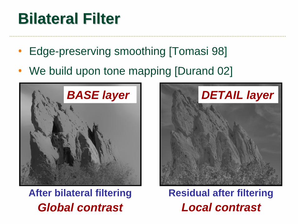
Bilateral FilterBilateral Filter

• Edge-preserving smoothing [Tomasi 98]

• We build upon tone mapping [Durand 02]

After bilateral filtering Residual after filtering

BASE layer DETAIL layer

Global contrast Local contrast

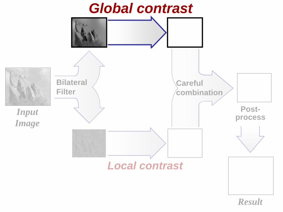
Global contrast

Input Image

Result

Careful combination

Post- process

Bilateral Filter

Local contrast

Local contrast

Global contrast

Input Image

Result

Careful combination

Post- process

Bilateral Filter

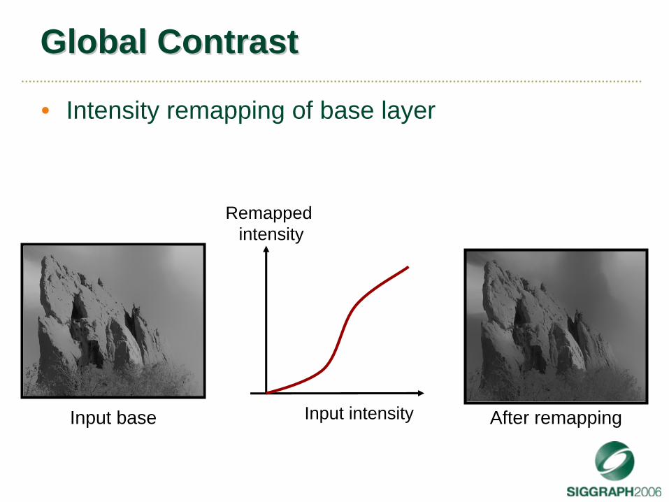
Global ContrastGlobal Contrast

• Intensity remapping of base layer

Input base After remappingInput intensity

Remapped intensity

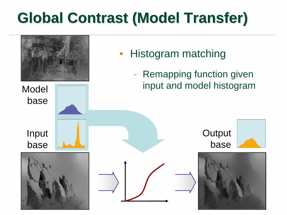
Global Contrast (Model Transfer)Global Contrast (Model Transfer)

• Histogram matching

- Remapping function given input and model histogramModel

base

Input base

Output base

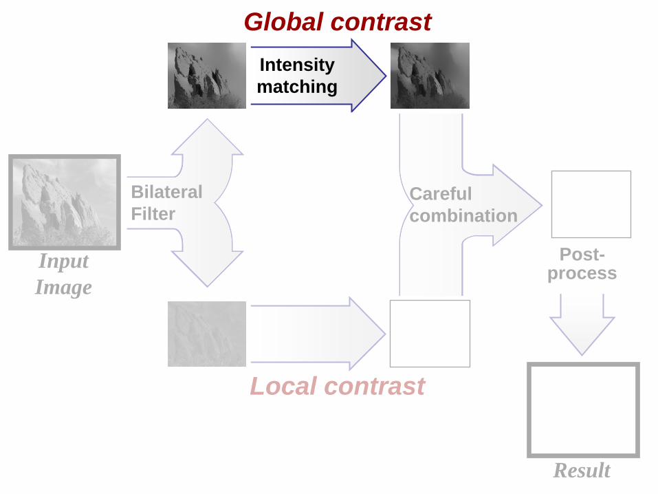
Local contrast

Global contrast

Input Image

Result

Careful combination

Post- process

Bilateral Filter

Intensity matching

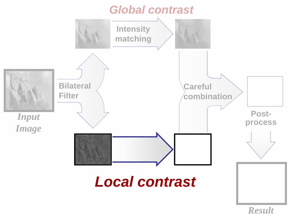
Local contrast

Global contrast

Input Image

Result

Careful combination

Post- process

Bilateral Filter

Intensity matching

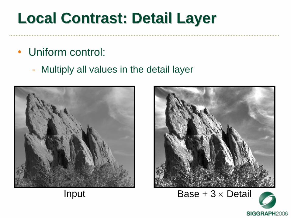
Local Contrast: Detail LayerLocal Contrast: Detail Layer

• Uniform control:- Multiply all values in the detail layer

Input Base + 3 ×

Detail

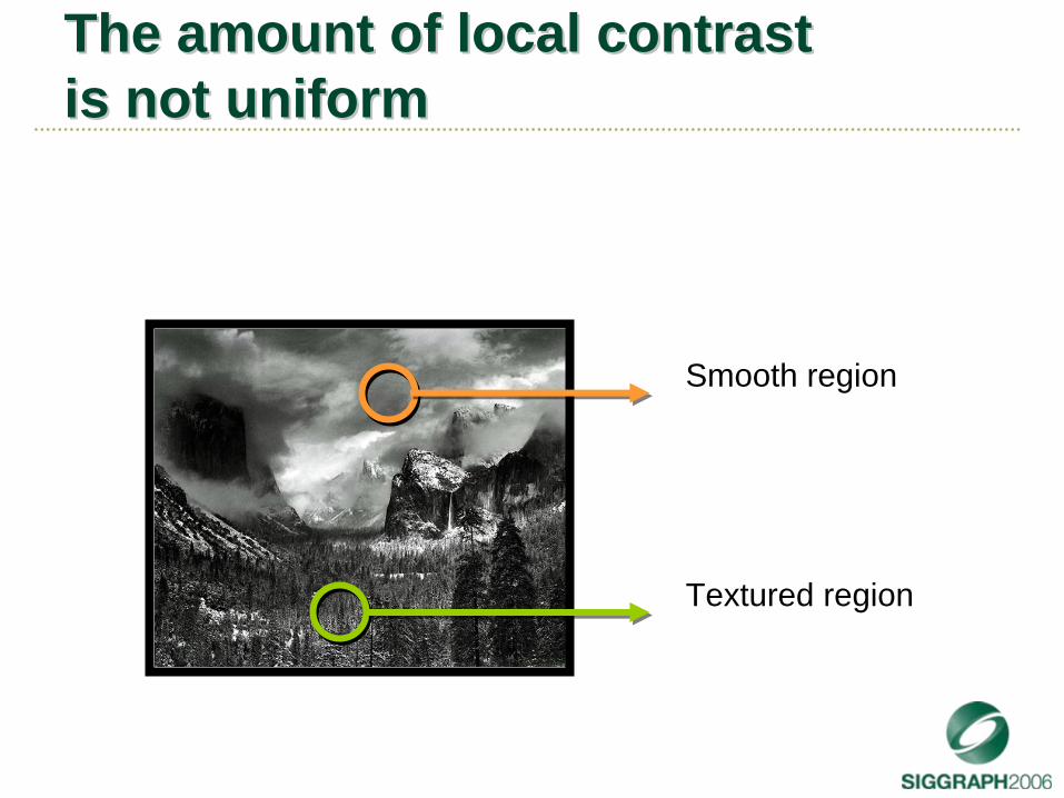
The amount of local contrast The amount of local contrast is not uniformis not uniform

Smooth region

Textured region

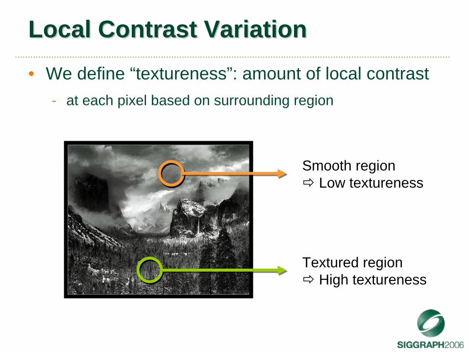
Local Contrast VariationLocal Contrast Variation

• We define “textureness”: amount of local contrast- at each pixel based on surrounding region

Smooth regionLow textureness

Textured regionHigh textureness

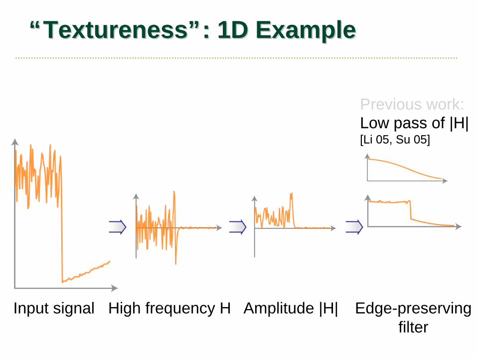
Input signal

““TexturenessTextureness””: 1D Example: 1D Example

High frequency H Amplitude |H| Edge-preserving filter

Previous work: Low pass of |H|[Li 05, Su 05]Low pass of |H|[Li 05, Su 05]

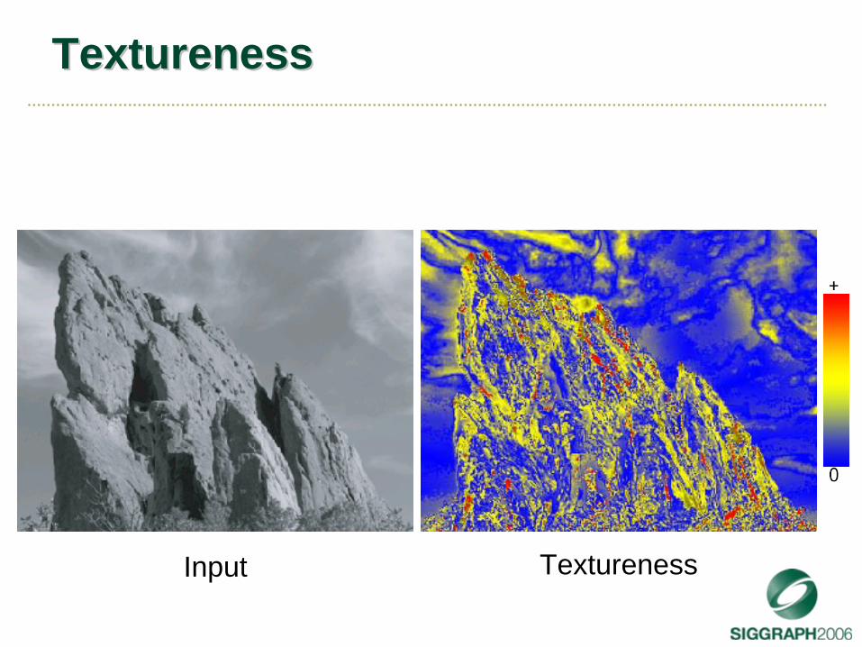
TexturenessTextureness

Input Textureness

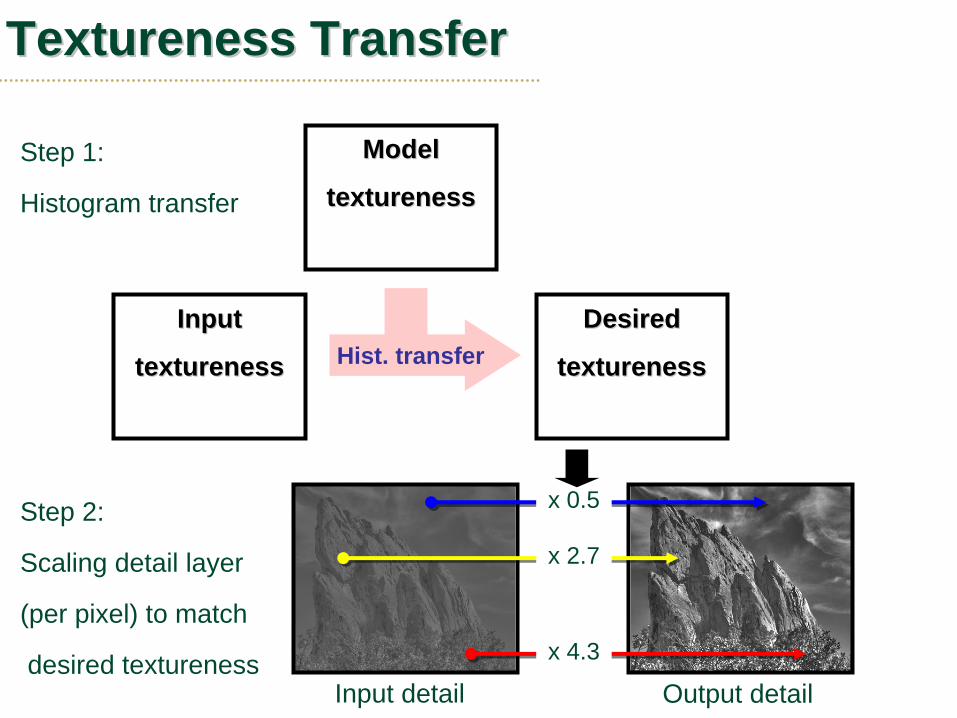
TexturenessTextureness TransferTransfer

Step 1:

Histogram transfer

Hist. transferInput Input

texturenesstextureness

Desired Desired

texturenesstextureness

Model Model

texturenesstextureness

x 0.5

x 2.7

x 4.3

Input detail Output detail

Step 2:

Scaling detail layer

(per pixel) to match

desired textureness

Local contrast

Global contrast

Input Image

Result

Careful combination

Post- process

Bilateral Filter

Intensity matching

Textureness matching

Local contrast

Global contrast

Input Image

Result

Careful combination

Post- process

Bilateral Filter

Intensity matching

Textureness matching

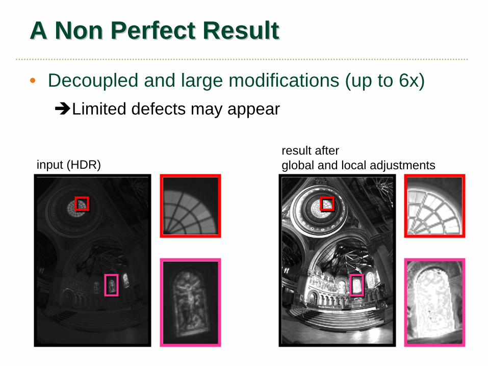
A Non Perfect ResultA Non Perfect Result

• Decoupled and large modifications (up to 6x)Limited defects may appear

input (HDR)result after global and local adjustments

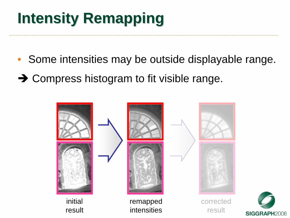
Intensity RemappingIntensity Remapping

• Some intensities may be outside displayable range.

Compress histogram to fit visible range.

corrected result

remapped intensities

initial result

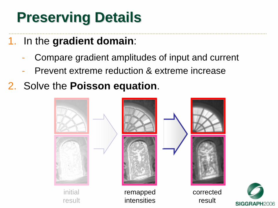
Preserving DetailsPreserving Details1. In the gradient domain:

- Compare gradient amplitudes of input and current- Prevent extreme reduction & extreme increase

2. Solve the Poisson equation.

corrected result

remapped intensities

initial result

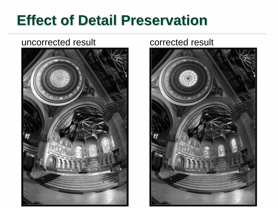
Effect of Detail PreservationEffect of Detail Preservationuncorrected result corrected result

Local contrast

Global contrast

Input Image

Result

Post- process

Bilateral Filter

Intensity matching

Textureness matching

Constrained Poisson

Local contrast

Global contrast

Input Image

Result

Bilateral Filter

Intensity matching

Textureness matching

Constrained Poisson

Post- process

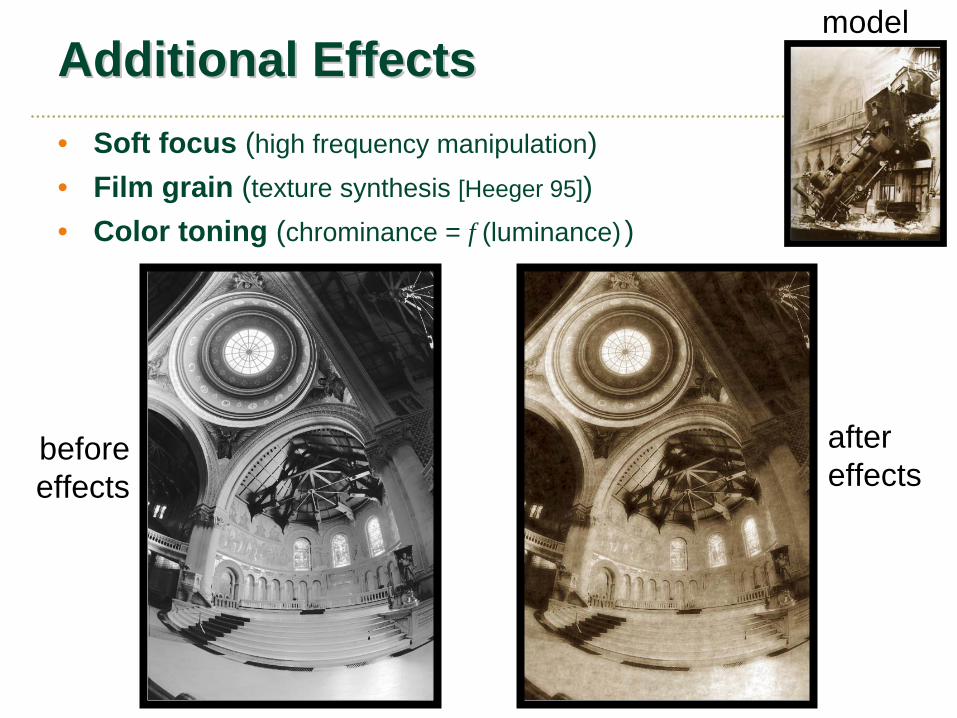
Additional EffectsAdditional Effects• Soft focus (high frequency manipulation)• Film grain (texture synthesis [Heeger 95])• Color toning (chrominance = f (luminance) )

before effects

after effects

model

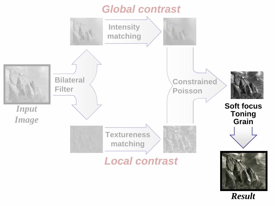
Intensity matching

Bilateral Filter

Local contrast

Global contrast

Input Image

Result

Textureness matching

Constrained Poisson

Soft focusToningGrain

Intensity matching

Bilateral Filter

Local contrast

Global contrast

Input Image

Result

Textureness matching

Constrained Poisson

Soft focusToningGrain

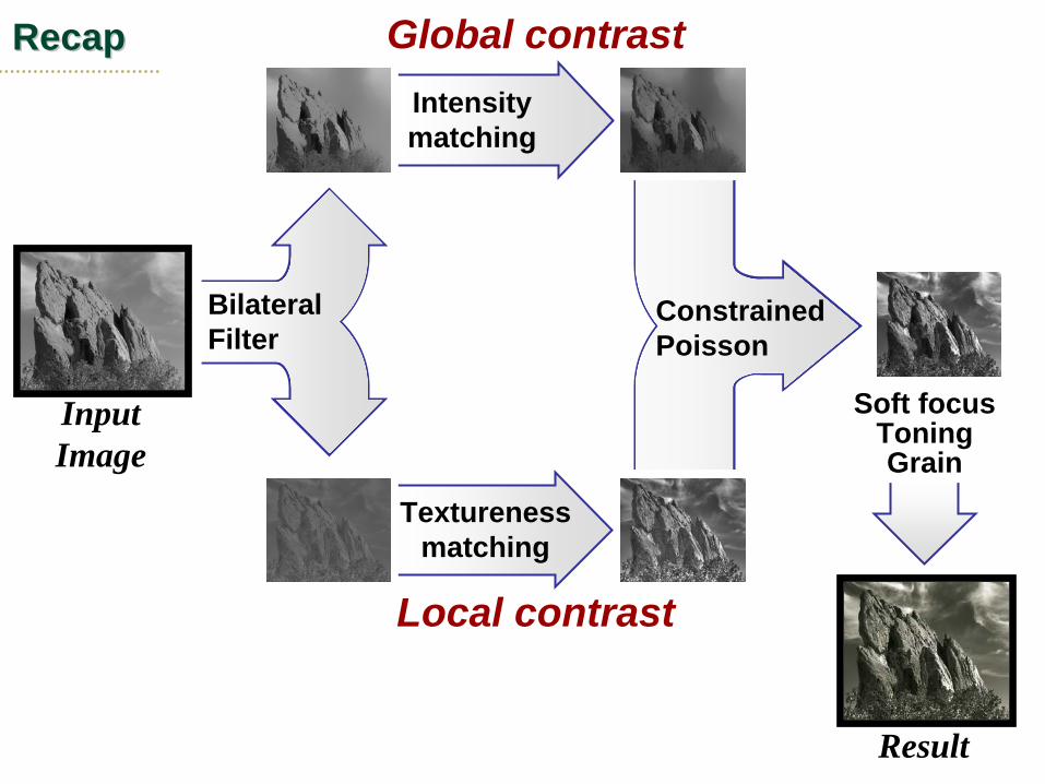
RecapRecap

ResultsResults

User provides input and model photographs.

Our system automatically produces the result.

Running times:- 6 seconds for 1 MPixel or less- 23 seconds for 4 MPixels

multi-grid Poisson solver and fast bilateral filter [Paris 06]

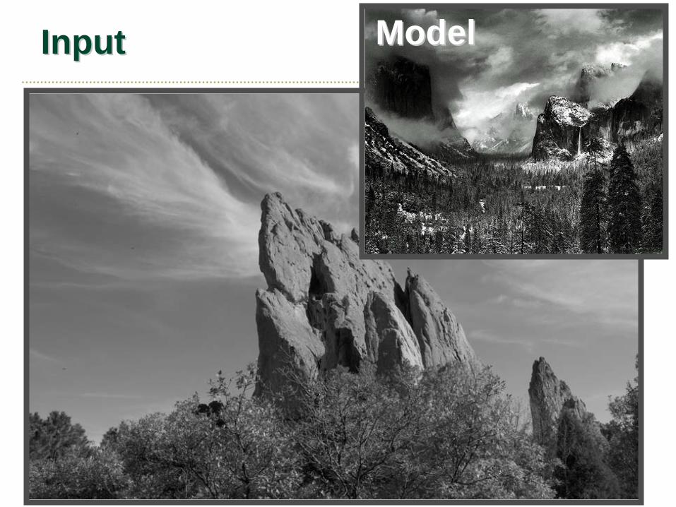
InputInput ModelModel

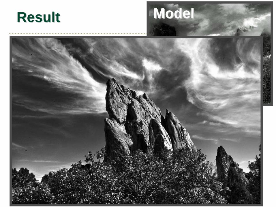
ResultResult ModelModel

InputInput

ResultResult

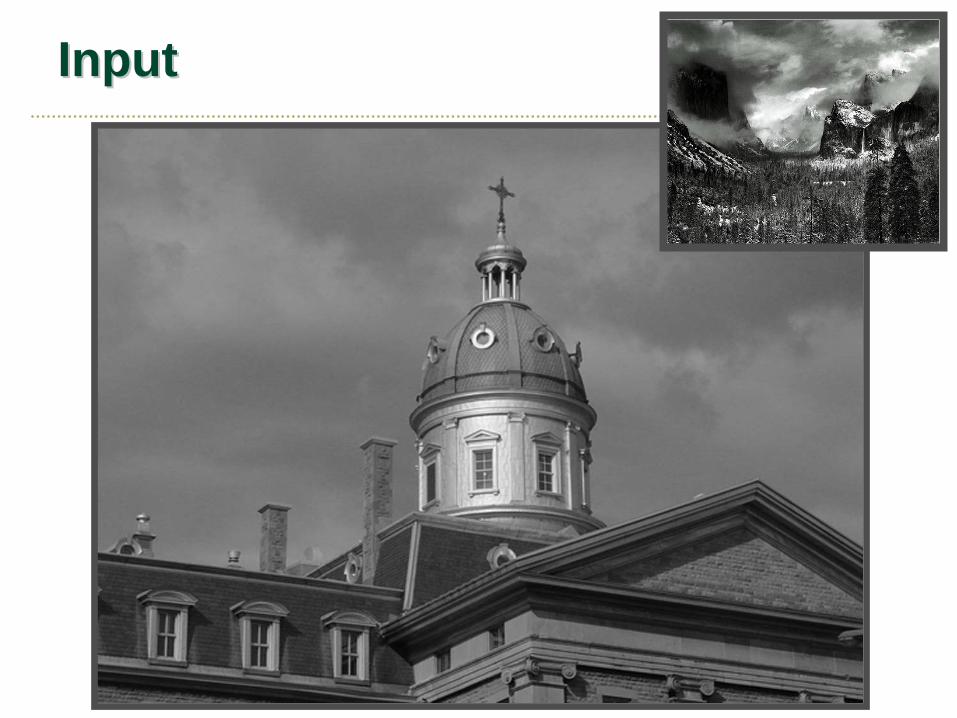
InputInput ModelModel

ResultResult ModelModel

InputInput

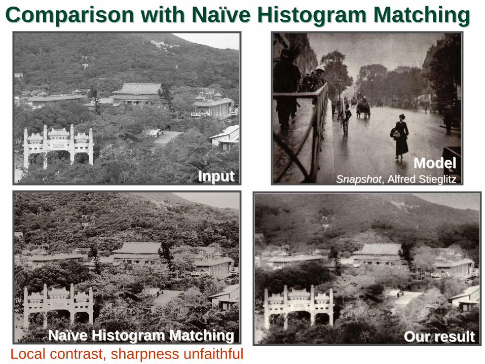
Our resultOur resultNaNaïïve Histogram Matchingve Histogram Matching

ModelModelSnapshotSnapshot, Alfred Stieglitz, Alfred Stieglitz

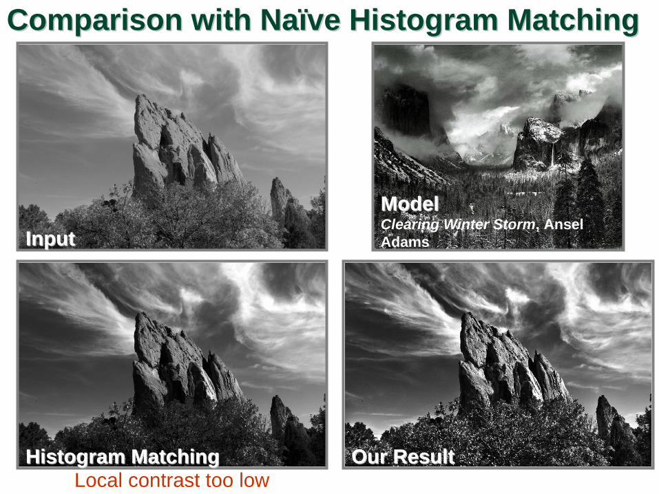
Comparison with NaComparison with Naïïve Histogram Matchingve Histogram Matching

Local contrast, sharpness unfaithful

InputInput

Our ResultOur Result

ModelModelClearing Winter Storm, Ansel Adams

Histogram MatchingHistogram Matching

Comparison with NaComparison with Naïïve Histogram Matchingve Histogram Matching

Local contrast too low

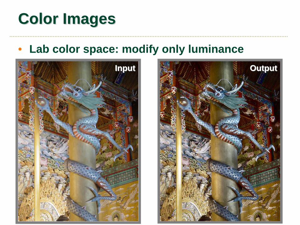
Color ImagesColor Images

• Lab color space: modify only luminanceInputInput OutputOutput

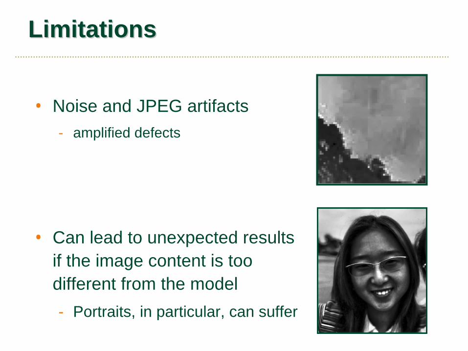
LimitationsLimitations

• Noise and JPEG artifacts - amplified defects

• Can lead to unexpected results if the image content is too different from the model- Portraits, in particular, can suffer

ConclusionsConclusions

• Transfer “look” from a model photo

• Two-scale tone management- Global and local contrast- New edge-preserving textureness- Constrained Poisson reconstruction- Additional effects