
1
Two‐Way Factorial ANOVA with R
This section will illustrate a factorial ANOVA where there are more than two levels
within a variable. The data I will be using in this section are adapted from a dataset called
“ChickWeight” from the R statistical program built-in package. These data provide the
complex analysis that I want to show here, but I have renamed the dataset in order to
better help you understand the types of analyses that we would do in second language
research. I call this dataset “Writing.txt,” and we will pretend that this data describes an
experiment that investigated the role of L1 background and experimental condition on
scores on a writing sample. The file is a .csv file, not an SPSS one.
The dependent variable in this dataset is the score on the writing assessment, which
ranges from 35 to 373 (pretend this is an aggregated score from four separate judges who
each rated the writing samples on a 100-point score). The independent variables are L1
(four L1s: Arabic, Japanese, Russian, and Spanish) and Condition. There were three
conditions that students were asked to write their essays in—“correctAll,” which means
they were told their teachers would correct all of their errors; “correctTarget,” which
means the writers were told only specific targeted errors would be corrected; and
“noCorrect,” in which nothing about correction was mentioned to the students.
First of all, we want to examine the data before running any tests, so Table 1 gives a
numerical summary of the data. The very highest scores within each L1 were obtained in
the condition where no corrections were made, and the lowest scores in the condition
where writers were told everything would be corrected. Standard deviations certainly

2
have a large amount of variation within each L1. The numbers of participants in each
group are unbalanced but there are a large number of them at least.
Table 1 Descriptive Statistics for the Writing Dataset.
Next, graphics will help in visually getting a feel for the multivariate data. Let’s look at
data using both of the graphics plots that I introduced in this chapter. First, the interaction
plot:
library(phia)
wmodel1<-lm(score~L1*condition, data=writing)
writing.mean<-interactionMeans(wmodel1)
plot(writing.mean)
The code above will give us the interaction plot in Figure 1. The top right panel of the
interaction plot quickly shows shows that all of the L1s performed similarly in the
different conditions (lines are mostly parallel), with the Russian and Spanish speakers
performing with the highest scores, and the Arabic speakers with the lowest scores. The

3
bottom left panel shows that there may be an interaction between L1 and condition,
because while in the correctAll condition there was little difference between L1s, in the
correctAll condition there seemed to be great differences between L1s. It also shows in
the main effect panels (top left and bottom right) that Spanish speakers did best overall,
and that that those who were not told anything about correction got the highest overall
scores (noCorrect) and those who were told everything would be corrected (correctAll)
got the most depressed scores.

4
Figure 1 Interaction plot from phia package with Writing dataset.
Next, let’s look at an interaction plot with boxplots for main effects:
library(HH)
interaction2wt(score~L1*condition,data=writing) #this is the basic command,
#although I did alter it a bit for readability

5
Figure 2 Interaction and boxplot from HH package with Writing dataset.
The interaction plots in Figure 2 don’t tell us any more than the ones in Figure 1, but I
like the boxplots because we can see that the data are not normally distributed (there are
outliers, represented by dots outside the maximum lines of the boxplots, and the
distribution is not symmetrical) and variances are certainly not equal for Condition, as the
amount of variation for the correctAll condition is quite low while for the noCorrect it is

6
quite large.
In the first edition of the book I published a barplot for these same data. This is
reproduced now in Figure 3. You can see that a barplot is not nearly as informative as
either of these graphics for this data.
Figure 3 Barplot of Writing dataset.

7
Calling for a two‐way factorial ANOVA In R Commander, open the writing.csv file by going to DATA > IMPORT DATA > FROM
TEXT FILE, CLIPBOARD, OR URL . . . . Enter the name writing for this file, and change the
“Field Separator” to “Commas.” Navigate to the file and open it, verifying that it has 3
columns and 578 rows. We’ll be working with this file from now on, so let’s go ahead
and attach it to our workspace. To get descriptive statistics such as were shown in Table
11.12, you could use the tapply( ) command with the two independent variables of L1
and condition on the response (dependent) variable of score, like this:
attach(Writing)
tapply(score,list(L1,condition),mean) #use sd and function(x) sum(!is.na(x)) instead
of mean to get standard
deviation and counts
Now we will begin to model. We can use either aov( ) or lm( ) commands, it makes no
difference in the end. Using the summary call for aov( ) will result in an ANOVA table,
while the summary for lm( ) will result in parameter estimates and standard errors (what I
call regression output). However, you can easily switch to the other form by using either
summary.lm( ) or summary.aov( ). In order to illustrate a different method than before,
I will be focusing on the regression output, so I will model with lm( ). I will illustrate the
“old statistics” point estimation model first before looking at confidence intervals.

8
An initial full factor ANOVA is called with the following call:
write=lm(score~L1*condition)
Anova(write)
The ANOVA shows that the main effect of first language, the main effect of condition,
and the interaction of L1 and condition are statistical. Remember, however, that when
interactions are statistical we are more interested in what is happening in the interaction
and the main effects are not as important. Thus, we now know that scores are affected by
the combination of both first language and condition, but we still need to know in more
detail how L1 and condition affect scores. This is when we will need to perform
comparisons.
We’ll start by looking at a summary of the model (notice that this is the regression output
summary, because I modeled with lm( ) instead of aov( ).
summary(write)

9
This output is considerably more complex than the ANOVA tables we’ve seen before, so
let’s go through what this output means. In the parameter estimate (regression) version of
the output, the factor levels are compared to the first level of the factor, which will be
whatever comes first alphabetically (unless you have specifically ordered the levels). To
see what the first level is, examine it with the levels command:
levels(L1)
[1] "Arabic" "Japanese" "Russian" "Spanish"
Thus, the row labeled L1[T.Japanese] compares the Arabic group with the Japanese
group because it compares the first level of L1 (Arabic) to the level indicated. The first
level of condition is allCorrect. The Intercept estimate shows that the overall mean score
on the writing sample for Arabic speakers in the allCorrect condition is 48.2 points, and
10
Japanese learners in the allCorrect condition score, on average, 1.7 points above the
Arabic speakers (that is what the Estimate for L1[T.Japanese] shows). The first 3 rows
after the intercept show, then, that no group is statistically different from the Arabic
speakers in the allCorrect condition. The next 2 rows, with “condition” at the beginning,
are comparing the correctTarget and noCorrect condition each with the noCorrect
condition, and both of these comparisons are statistical. The last 6 rows of the output
compare various L1 groups in either the correctTarget condition or the noCorrect
condition with the Arabic speakers in the allCorrect condition (remember, this is the
default level). Thus, the last 6 lines tell us that there is a difference between the Russian
speakers in the correctTarget condition with the Arabic speakers in the allCorrect
condition, and also that all L1 speakers are statistically different in the noCorrect
condition from the Arabic speakers in the allCorrect condition.
At this point, you may be thinking this is really complicated and you really didn’t want
comparisons only with Arabic or only in the allCorrect condition. What can you do to
get the type of post-hoc tests you would find in a commercial statistical program like
SPSS which can compare all levels? The pairwise.t.test( ) command can perform all
possible pairwise comparisons if that is what you would like.
For example, we can look at comparisons only between the L1s and see a p-value for
these comparisons:
pairwise.t.test(score,L1, p.adjust.method="fdr")

11
This shows that overall, Arabic L1 speakers are different from all the other groups; the
Japanese L1 speakers are different from the Spanish L1 speakers, but not the Russian L1
speakers. Lastly, the Russian speakers are not different from the Spanish speakers. We
can also look at the comparisons between conditions:
pairwise.t.test(score,condition, p.adjust.method="fdr")
Here we see very low p-values for all conditions, meaning all conditions are different
from each other. Lastly, we can look at comparisons on the interaction:
pairwise.t.test(score,L1:condition, p.adjust.method="fdr")
This is only the beginning of a very long chart . . .

12
Going down the first column, it’s clear that none of the groups are different from the
Arabic L1 speakers in the correctAll condition (comparing Arabic to Japanese p=.87,
Arabic to Russian p=.69, Arabic Spanish p=.80). That, of course, doesn’t tell us
everything; for example, we don’t know whether the Japanese speakers are different from
the Russian and Spanish speakers in the correctAll condition, but given our graphics in
Figures 1 to 4, we might assume they will be when we check. Looking over the entire
chart we get a full picture of the nature of the interaction: no groups are different from
each other in the correctAll condition; in the correctTarget condition, only the Russian
and Arabic and the Spanish and Arabic speakers differ statistically from each other; in the
noCorrect condition, all groups perform differently from one another.
Here is the analysis of the post-hoc command in R:
pairwise.t.test(score,L1:condition, p.adjust.method="fdr") pairwise.t.test(score, . . . Put in the dependent (response) variable as the
first argument L1:condition The second argument is the variable containing
the levels you want compared; here, I didn’t care about the main effects of L1 or condition, just the interaction between them, so I put the interaction as the second argument
p.adjust.method="fdr" Specifies the method of adjusting p-values for multiple tests; you can choose hochberg, hommel, bonferroni, BH, BY, and none (equal to LSD); I chose fdr because it gives more power while still controlling for type I error
Now that we’ve seen how to look at this comparison by only using p-values, let’s look at
how we could instead examine confidence intervals. Since we only have two variables we

13
do not need to subset the data, as we did in Section 10.5.2 of the book, and can instead go
straight to using the multcomp package and the syntax used there to create a coefficient
matrix that will test all of the comparisons between groups. This syntax will be a little
different from the syntax used in Section 10.5.2 because each variable has more than 2
levels. If you can understand the syntax you can understand how you would need to
change the syntax to fit your own situation with the number of levels in each variable that
you have. I have added a number of annotations in the syntax to help you, but you’ll
understand best if you work through the example and look at each object that you create
after you make it as you go along.
The following syntax creates a contrax matrix for L1 for each level of condition (N.B.
items in red should be replaced with your own data name):
Tip: How do I change this syntax for my own data? The basic idea is that comparisons will be made among the levels of the first variable that you enter (L1 for my writing dataset; since there are four levels of L1, there are 6 comparisons). Then you will need to make matrices that will be of size 6 rows × 4 columns, so you see the number of rows is the number of comparisons among the IV entered first (L1 for my data) and the number of columns is the number of levels in that same IV (L1). But you will need to repeat this matrix 3 times. That is because there are 3 levels of condition. Repeating three times also has to happen in two places: 1) In the width of the matrix K, and in the number of K that need to be created. That is why in the syntax below I had to: 1) Put in 3 sets of 6 rows × 4 column matrices, 2 with only zeros and 1 with the +1s and -1s necessary to call for the correct contrasts, whereas in Section 10.5.2 of the book I only had 2 sets of 2 rows × 2 column matrices and 2) Create 3 sets of K (K1, K2, K3) whereas in Section 10.5.2 I only created 2 (because there were only 2 levels of my IV).

14
library(multcomp)
names(writing)
Tukey=contrMat(table(writing$L1),"Tukey")
K1=cbind(Tukey, matrix(0,nrow=nrow(Tukey), ncol=ncol(Tukey)),
matrix(0,nrow=nrow(Tukey), ncol=ncol(Tukey))) #there are 3 levels of condition, so
#we bind together 3 matrices of 4 columns
#the 4 columns are because there are 4 columns in the Tukey matrix from L1
#the +1 and -1 are in the first matrix of 4 columns, where Tukey is
rownames(K1)=paste(levels(writing$condition)[1], rownames(K1), sep=":")
K2=cbind(matrix(0,nrow=nrow(Tukey),ncol=ncol(Tukey)),Tukey,
matrix(0,nrow=nrow(Tukey), ncol=ncol(Tukey)))
#the +1 and -1 are in the second matrix of 4 columns, where Tukey is
rownames(K2)=paste(levels(writing $condition)[2],rownames(K2),sep=":")
K3=cbind(matrix(0,nrow=nrow(Tukey),ncol=ncol(Tukey)),
matrix(0,nrow=nrow(Tukey),ncol=ncol(Tukey)), Tukey) #a third matrix is needed
#because there are 3 levels of condition
#the +1 and -1 are in the third matrix of 4 columns, where Tukey is
rownames(K3)=paste(levels(writing$condition)[3],rownames(K3),sep=":")
K=rbind(K1, K2,K3)
colnames(K)=c(colnames(Tukey), colnames(Tukey), colnames(Tukey))
#we have 3 matrices of 4 columns each so we have to repeat the column names 3 times
writing$L1C=with(writing, interaction(L1,condition))
cell=lm(score~L1C-1, data=writing)
15
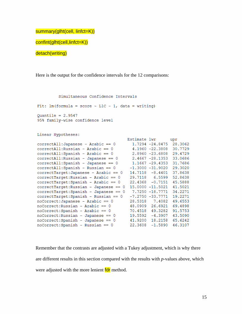
summary(glht(cell, linfct=K))
confint(glht(cell,linfct=K))
detach(writing)
Here is the output for the confidence intervals for the 12 comparisons:
Remember that the contrasts are adjusted with a Tukey adjustment, which is why there
are different results in this section compared with the results with p-values above, which
were adjusted with the more lenient fdr method.

16
Another nice thing to do here is to plot the confidence intervals on a graph:
par(mar=c(4,14,4,2))#adjusts margin parameters to make left margin large enough for
#labels
#default margins are (5,4,4,2) and you might want to set them back to normal after
#printing
plot(glht(cell,linfct=K))
17
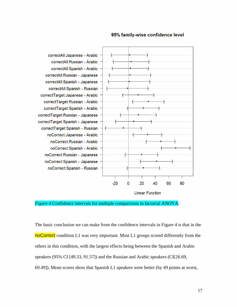
Figure 4 Confidence intervals for multiple comparisons in factorial ANOVA.
The basic conclusion we can make from the confidence intervals in Figure 4 is that in the
noCorrect condition L1 was very important. Most L1 groups scored differently from the
others in this condition, with the largest effects being between the Spanish and Arabic
speakers (95% CI [49.33, 91.57]) and the Russian and Arabic speakers (CI[26.69,
69.49]). Mean scores show that Spanish L1 speakers were better (by 49 points at worst,

18
perhaps 91 points at best) than the Arabic speakers, and that the Russian L1 speakers
were better than the Arabic L1 by 27 points at least, and possibly as much as 69 points.
The confidence intervals were quite wide in all cases, however, and for some
comparisons in the noCorrect condition the CI was very close to zero, such as for the
comparison between Arabic L1 and Japanese L1 speakers, with a mean difference of 28.5
points and CI of [-49.85, -7.5], with mean scores showing the Japanese did better than the
Arabic speakers. In other cases, we could not be sure of any real effect as the CI went
through zero, as for the comparison between Russian L1 and Japanese L1 speakers,
although this confidence interval was not centered around zero and with a more precision
may have shown a weak effect. For the correctTarget and correctAll conditions, L1 was
not very important, as most comparisons (except one) did not show any effect for L1.
Of course, this is not nearly the end of the analysis one could do, and in reporting on the
results I would want to present descriptive statistics of mean scores, estimates of mean
differences between groups, and confidence intervals for a full complement of
comparisons, not just the ones where there was an effect. This is true whether you report
CIs or p-values.
However, it would be the end of my investigation of this dataset. Since I found two-way
interactions with real effects, I would not be interested in looking at the main effects of
just L1 or just Condition. Stop looking at lower-order comparisons if you find effects at
the higher level. In other words, if you find real effects for a two-way comparison, do not
bother to look at main effects (the levels of one variable). If you need to examine main
effects, use techniques for one-way ANOVAs if there are more than two levels, or

19
techniques for t-tests if there are only two levels.
We’ve been able to answer our question about how the levels of the groups differ from
one another, but we have had to perform a large number of post-hoc tests. If we didn’t
really care about the answers to all the questions, we have wasted some power by
performing so many. One way to avoid such a large number of post-hoc tests would be to
have planned out your question in advance and to run a priori planned comparisons.
Robust Methods of Performing Factorial ANOVA in R In this section I will provide explanation of some of Wilcox’s (2005) robust methods for
two-way and three-way ANOVAs. Before using these commands you will need to load
Wilcox’s package, WRS, into R (see Section 8.4.4 in the book for a complete list of what
to install) and then open Wilcox’s WRS package (library(WRS)). Wilcox recommends a
bootstrap-t method when comparing means or trimmed means with a small amount of
trimming (20% is the default), especially when sample sizes are small, while a percentile
bootstrap is better when comparing groups based on other measures of location that are
not means (such as M-estimators or MOM).
The command t2waybt( ) uses trimmed means and a bootstrap-t for a two-way ANOVA,
the command t3waybt( ) uses trimmed means and a bootstrap-t for a three-way ANOVA,
and the command pbad2way( ) uses the percentile bootstrap and M-measures of location
(not means) in a two-way design. For all of these tests, the data need to be stored in a
matrix or list. The WRS command fac2list(x, g) takes the response variable data in x and
20
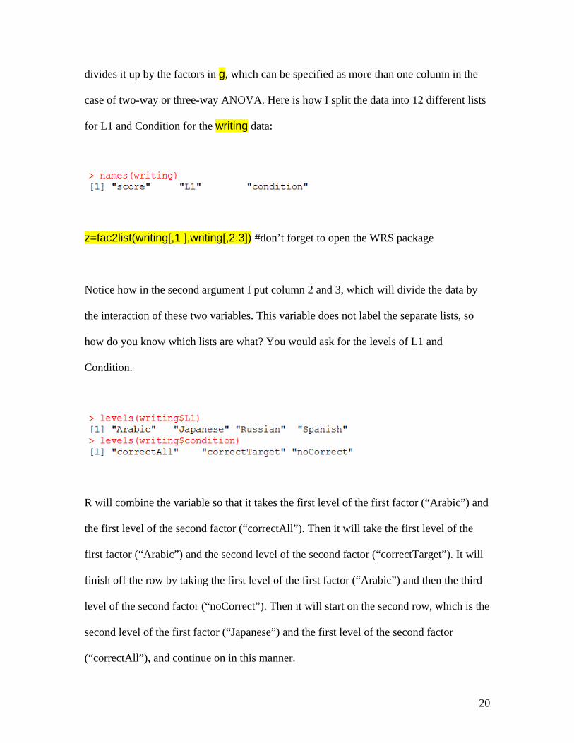
divides it up by the factors in g, which can be specified as more than one column in the
case of two-way or three-way ANOVA. Here is how I split the data into 12 different lists
for L1 and Condition for the writing data:
z=fac2list(writing[,1 ],writing[,2:3]) #don’t forget to open the WRS package
Notice how in the second argument I put column 2 and 3, which will divide the data by
the interaction of these two variables. This variable does not label the separate lists, so
how do you know which lists are what? You would ask for the levels of L1 and
Condition.
R will combine the variable so that it takes the first level of the first factor (“Arabic”) and
the first level of the second factor (“correctAll”). Then it will take the first level of the
first factor (“Arabic”) and the second level of the second factor (“correctTarget”). It will
finish off the row by taking the first level of the first factor (“Arabic”) and then the third
level of the second factor (“noCorrect”). Then it will start on the second row, which is the
second level of the first factor (“Japanese”) and the first level of the second factor
(“correctAll”), and continue on in this manner.

21
If you have your data already in the wide format where each column represents the
response variable divided by your independent variables, there is no need to put it into a
list. Instead, you can tell the command what order to take the columns in by specifying
for grp, like this:
grp<-c(2,3,5,8,4,1,6,7)
where column 2 (as denoted by c(2)) is the data for level 1 of Factors A and B, column 3
is the data for level 1 of Factor A and level 2 of Factor B, etc. (do rows first, columns
second).
Now that the data are in the correct form I can run the t2waybt( ) test. Here is the basic
syntax:
t2waybt(J, K, x, tr=0.2, grp=c(1:p), p=J*K, nboot=599, SEED=T)
where J= the number of levels of the first variable used in whatever you have made that
specifies groups (we made z, where the first variable was Pictures), K= the number of
levels of the second variable, tr is the amount of trimming (default 20%), x is the place
where the data is stored, grp specifies the groups if you need to specify them in an order
different from the way they are listed in x or if they are a subset of x, and where p is
something you can ignore as it works out whether the total number of groups is correct.

22
Leave nboot as it is for now, and SEED is something you should only use if you want to
be able to replicate a particular run of the command with the bootstrap. Now I run the
command with the writing data:
t2way(4,3,z,tr=.2) #the output is skinny so I am going to rearrange it to fit better on my
#page
The output from this test returns the test statistic Q for Factor A (which is L1 here) in the
$Qa line, and the p-value for this test in the $A.p.value line. So the factor of L1 is
statistical, p=.001. So is the factor of Condition, listed as $Qb (p=.001), and also the
interaction between the two is statistical, listed as $Qab (p=.001).
Great! We know we have a statistical interaction but now we need to perform multiple
comparisons to find out which levels are statistically different from one another. In this
case, use the linconb( ) command that uses the bootstrap-t and trimmed means, described
in Section 9.4.8. I will walk you through the steps.

23
w=con2way(4,3)
Create an object, w, that holds the contrasts for a 4 × 3 matrix. Make sure your first number specifies the levels of the first factor of your data in z (from above in this section, it is an object that holds our data and the independent variables)
linconb(z, con=w$conA, tr=.2) This will perform multiple comparisons of all of the interactions between the first variable (L1) with bootstrapping and means trimming of default 20%
The output is long, so I have cut it down to a sample:
The warning tells us the confidence intervals are adjusted to control for having multiple
comparisons (there are 18 in all) but the p-values (not shown) are not. In the part labeled
$n we get the number of participants in each group (not the number in each comparison
though). Which group is it? Remember that Group 1=Arabic_CorrectAll, Group
2=Arabic_CorrectTarget, Group 3=Arabic_noCorrect, Group 4=Japanese_CorrectAll,
and Group 5=Japanese_CorrectTarget, and so on.

24
Then under $psihat we get the difference between the two compared groups, and the
confidence level of that comparison. But what has been compared? For that, we need to
look at the last part of the output labeled $con:
To interpret this we need to understand how contrasts work. I first looked at contrasts in
Section 9.4.7 of the book, and most recently looked at them in Section 10.5.3 when doing
planned comparisons. If you understand how contrasts work, you can see that what was
compared in the first column of these contrasts was all of the Arabic speakers to the
Japanese speakers (because each one of the 3 condition contrasts for Arabic speakers got
a +1, and each one of the 3 condition contrasts for Arabic speakers got a -1). Column 2
describes the contrast between Arabic and Russian speakers, column 3 between Arabic
and Spanish speakers. Can you work the rest out?
Now go back and look at the confidence intervals (I’ve already discussed the results in
previous sections so won’t do so again here except to note that compared with non-
trimmed and non-bootstrapped comparisons in the first section (“Performing a two-way
factorial ANOVA”) of this document, there is a difference in the comparison between

25
Japanese and Russian speakers (the 4th row), which has a CI that does not pass through
zero here, although it is fairly close, whereas in the first section of this document the p-
value was higher than .05).
We should be able to also look at the comparison between all the levels of the two factors
in the w$conAB argument, but I found this to be a strange comparison the way it was set
up. In fact, Wilcox says that the AB comparison is between “all interactions associated
with any two rows and columns” (2011, p. 596), and in the contrasts we find 2 “1”s and 2
“-1”s, so that we are comparing CorrectAll:CorrectTarget::Arabic:Japanese, indeed, it
appears we are comparing two rows and two columns at the same time, but I am not sure
how to interpret this. Below is an example of what these contrasts look like (there are 18
columns but I am only showing 13).
Therefore, I cannot recommend this approach as a way to bootstrapping the comparisons
between the interaction.
26
For a two-way analysis using percentile bootstrapping and M-estimators, the command
pbad2way( ) can be used. The data need to be arranged in exactly the same way as for
the previous command, so we are ready to try this command out:
pbad2way(4,3,z,est=onestep, conall=T, alpha=.05, nboot=2000, grp=NA,
pro.dis=F) #If you needed it, you #could use the grp term as described previously to
specify certain groups
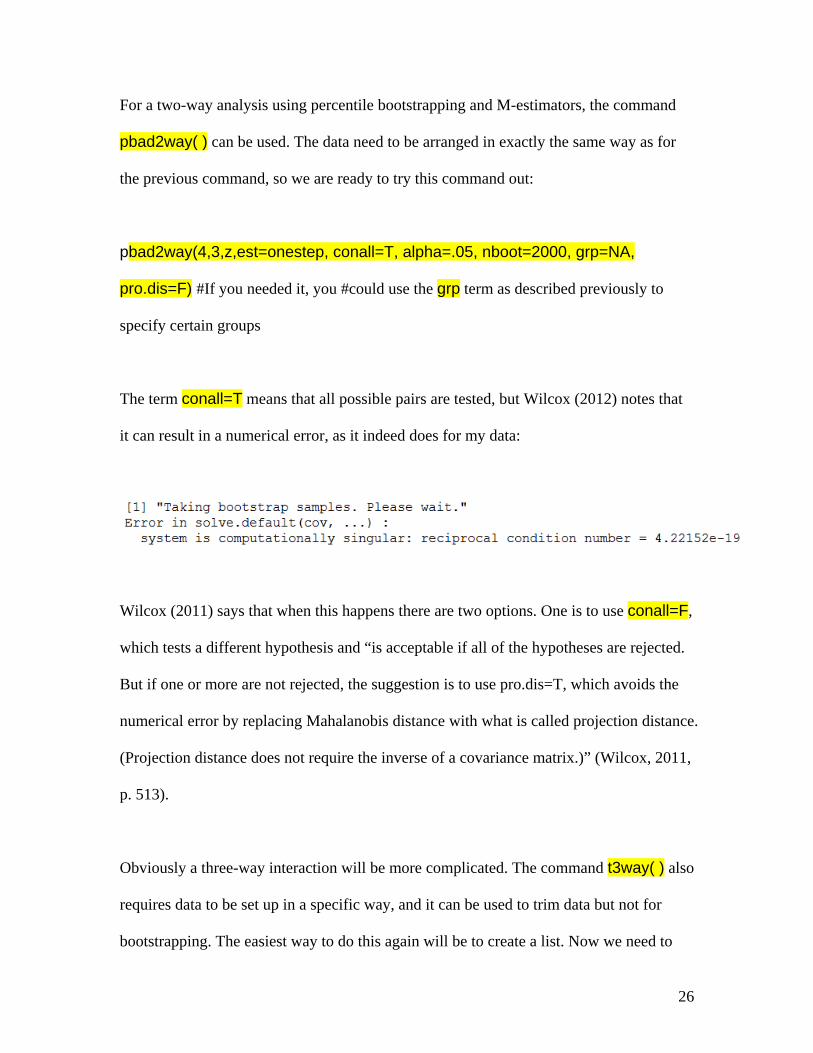
The term conall=T means that all possible pairs are tested, but Wilcox (2012) notes that
it can result in a numerical error, as it indeed does for my data:
Wilcox (2011) says that when this happens there are two options. One is to use conall=F,
which tests a different hypothesis and “is acceptable if all of the hypotheses are rejected.
But if one or more are not rejected, the suggestion is to use pro.dis=T, which avoids the
numerical error by replacing Mahalanobis distance with what is called projection distance.
(Projection distance does not require the inverse of a covariance matrix.)” (Wilcox, 2011,
p. 513).
Obviously a three-way interaction will be more complicated. The command t3way( ) also
requires data to be set up in a specific way, and it can be used to trim data but not for
bootstrapping. The easiest way to do this again will be to create a list. Now we need to

27
arrange the data so that for level 1 of Factor A, we will find the first vector of the list
contains level 1 for Factor B and level 1 for Factor C. The second vector will contain
level 1 for Factor A, level 1 for Factor B, and level 2 for Factor C. See Table 1 (taken
from Wilcox, 2005, p. 286) for more details on how a design of 2×2×4 would be set up:
Table 2 Data arranged for a three-way ANOVA command from Wilcox.
level 1 of
Factor A
Factor C
Factor B x[[1]] x[[2]] x[[3]] x[[4]]
x[[5]] x[[6]] x[[7]] x[[8]]
level 2 of
Factor A
Factor C
Factor B x[[9]] x[[10]] x[[11]] x[[12]]
x[[13]] x[[14]] x[[15]] x[[16]]
Let’s examine the Obarow data now, using a 2×2×2 design (so there will be 8 categories)
with Gender included as Factor C. Using the previous fac2list() command, we should be
able to arrange the data in an object y:

28
To understand the meaning of each contrast number, we’ll need to know how the levels
are arranged:
Now we can tell that group 1=male, no pictures, no music; group 2=male, no pictures,
music; group 3=male, pictures, no music and group 4=male, pictures, music (and just
repeat with female in place of male for groups 5-8). We’re ready to try the trimmed
means ANOVA test, which can especially help with heteroscedasticity, according to
Wilcox (2011).
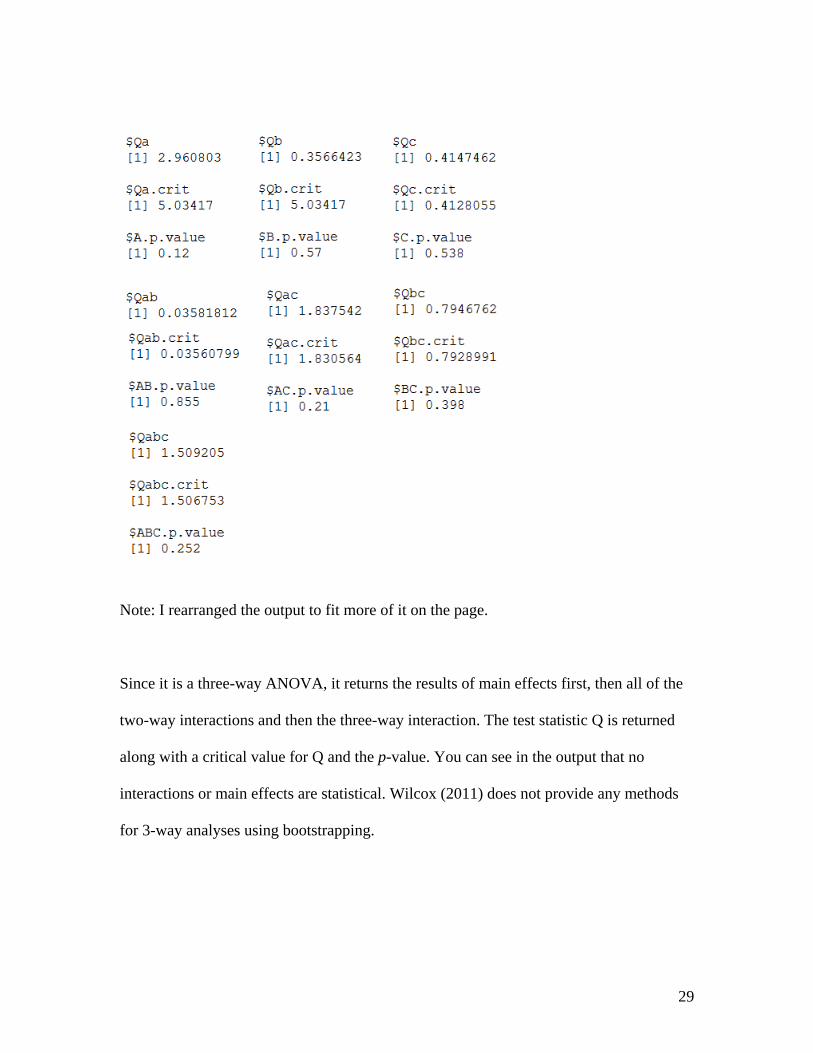
t3way(2,2,2, y, tr=.2) #If you need to, you can specify the grp argument as above
Note that A=Gender, B=Pictures, & C=Music; further, AB=Gender:Pictures,
AC=Gender:Music and BC=Pictures:Music.
29
Note: I rearranged the output to fit more of it on the page.
Since it is a three-way ANOVA, it returns the results of main effects first, then all of the
two-way interactions and then the three-way interaction. The test statistic Q is returned
along with a critical value for Q and the p-value. You can see in the output that no
interactions or main effects are statistical. Wilcox (2011) does not provide any methods
for 3-way analyses using bootstrapping.

30
Bibliography
Wilcox, R. (2005). Introduction to robust estimation and hypothesis testing. San
Francisco: Elsevier.
Wilcox, R. R. (2011). Modern statistics for the social and behavioral sciences: A
practical introduction. New York: Chapman & Hall/CRC Press.
Summary Performing Robust ANOVAs using Wilcox’s (2011) Commands
1 If your data is in the long form, rearrange data using Wilcox’s fac2list( ) command from the WRS package (N.B. items in red should be replaced with your own data name): z=fac2list(writing[,1 ],writing[,c(2,3)]) Specify the response (dependent) variable in the first argument and the independent variables in the second argument. Using the c( ) syntax you can list any columns you need.
2 To calculate a two-way trimmed means bootstrap-t ANOVA, use: t2waybt(J, K, z, tr=0.2, nboot=599) where J=# of levels for Factor A, K=# of levels for Factor B, z=data in correct format
3 To calculate a two-way percentile bootstrapping ANOVA using M-estimators, use: pbad2way(J,K,z,est=onestep, nboot=2000) This command may have problems with the covariance matrix; see text for details of how to fix
4 To calculate a three-way trimmed means ANOVA, use: t3way(J, K, L, z, tr=.2) where L= levels for Factor C


