

Nan Zang
Overview of the paper
Introduction
Classification
Complexity results for Pm | prec, pj = 1 | Cmax
Algorithms for Pk | prec, pj = 1 | Cmax
Future research directions and conclusions

Nan Zang
Scheduling
Scheduling concerns optimal allocation of scarce resources to activities.
For example Class scheduling problems
Courses Classrooms Teachers

Nan Zang
Problem notation (1)
A set of n jobs J = { J1, J2, ……, Jn}
The execution time of the job Jj is p(Jj).
A set of processors P = {P1 , P2, ……}
Schedule Specify which job should be executed by
which processor at what time.
Objective Optimize one or more performance criteria

Nan Zang
Problem Notation (2)
α describes the processor environment Number of processors, speed, …
β provides the job characteristics release time, precedence constraints, preemption,
…
γ represents the objective function to be optimized
The finishing time of the last job (makespan) The total waiting time of the jobs
3-field notation α|β|γ (Graham et al.)

Nan Zang
Job Characteristics
Release time (rj) - earliest time at which job Jj can start processing.
- available job
Preemption (prmp) - jobs can be interrupted during processing.
Precedence constraints (prec) - before certain jobs are allowed to start processing,
one or more jobs first have to be completed. - a ready job

Nan Zang
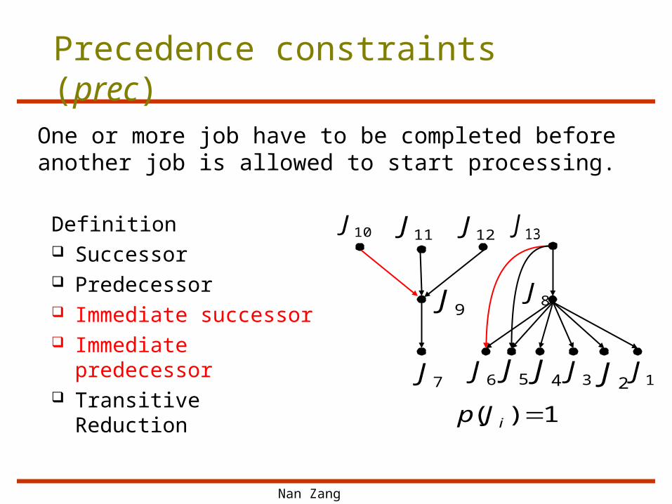
Precedence constraints (prec)
Definition Successor Predecessor Immediate successor Immediate
predecessor Transitive Reduction
Before certain jobs are allowed to start processing, one or more jobs first have to be completed.
10J 11J
9J
12J
7J
8J
6J 5J 4J 3J 2J 1J
1)( iJp
13J
Nan Zang
Precedence constraints (prec)
Definition Successor Predecessor Immediate successor Immediate
predecessor Transitive Reduction
One or more job have to be completed before another job is allowed to start processing.
10J 11J
9J
12J
7J
8J
6J 5J 4J 3J 2J 1J
1)( iJp
13J
Nan Zang
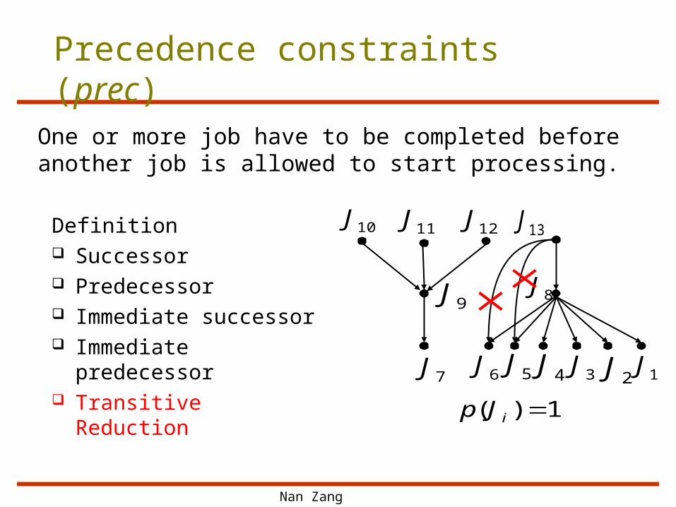
Precedence constraints (prec)
Definition Successor Predecessor Immediate successor Immediate
predecessor Transitive Reduction
One or more job have to be completed before another job is allowed to start processing.
10J 11J
9J
12J
7J
8J
6J 5J 4J 3J 2J 1J
1)( iJp
13J

Nan Zang
Special precedence constraints (1)
In-tree (Out-tree)
In-forest (Out-forest)
Opposing forest
Interval orders
Quasi-interval orders
Over-interval orders
Series-parallel orders
Level orders
Nan Zang
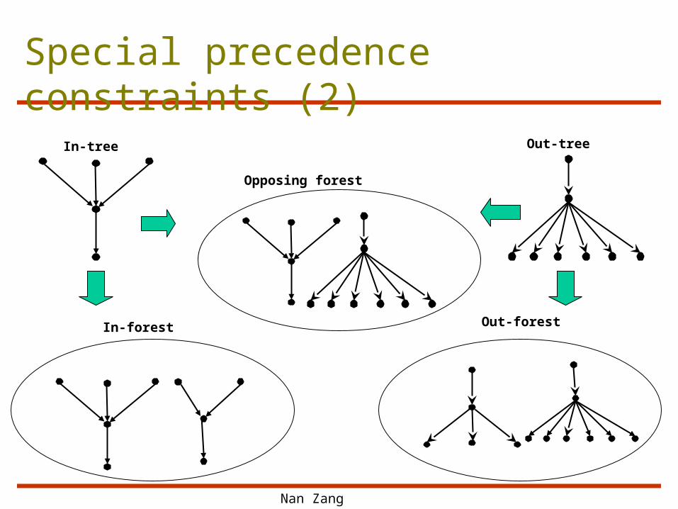
Special precedence constraints (2)
In-forest
Out-treeIn-tree
Out-forest
Opposing forest
Nan Zang
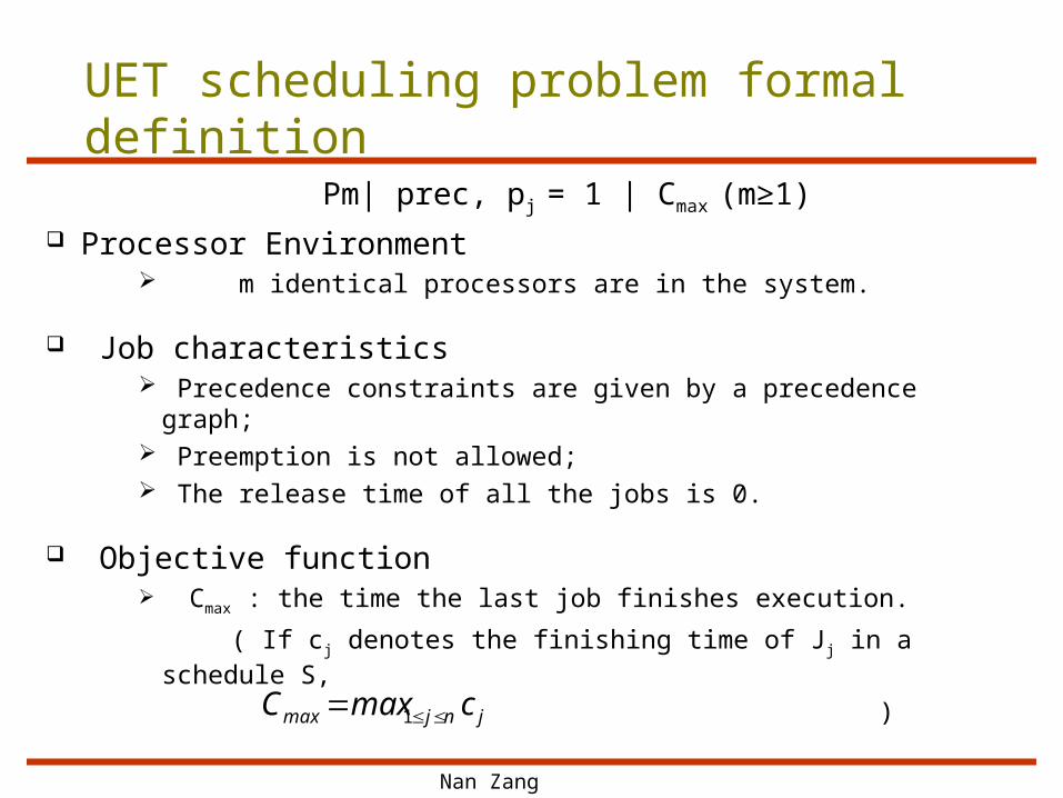
UET scheduling problem formal definition
Pm| prec, pj = 1 | Cmax (m≥1) Processor Environment
m identical processors are in the system.
Job characteristics Precedence constraints are given by a precedence
graph; Preemption is not allowed; The release time of all the jobs is 0.
Objective function Cmax : the time the last job finishes execution.
( If cj denotes the finishing time of Jj in a schedule S,
) jnjmax cmaxC 1

Nan Zang
Gantt Chart
15J14J
10J 11J
9J
12J
7J
8J
6J 5J 4J 3J 2J 1J
1)( iJp
13J
A Gantt chart indicates the time each
job spends in execution, as well as
the processor on which it executes
Time axis
P1
P2
P3 11J10J12J
9J13J
8J 7J
6J
5J
4J
3J
2J
1J
15J
14J
Slot 1 Slot 2
Nan Zang
Overview of the paper
Introduction
Classification
Complexity results for Pm | prec, pj = 1 | Cmax
Algorithms for Pk | prec, pj = 1 | Cmax
Future research directions and conclusions

Nan Zang
Classification
Due to the number of processors
Number of processors is a variable (m) Pm | prec, pj = 1 | Cmax
Number of processors is a constant (k) Pk | prec, pj = 1 | Cmax

Nan Zang
Classification
Due to the number of processors
Number of processors is a variable (m) Pm| prec, pj = 1 | Cmax
Number of processors is a constant (k) Pk| prec, pj = 1 | Cmax
Nan Zang
Pm| prec, pj = 1 | Cmax (1)
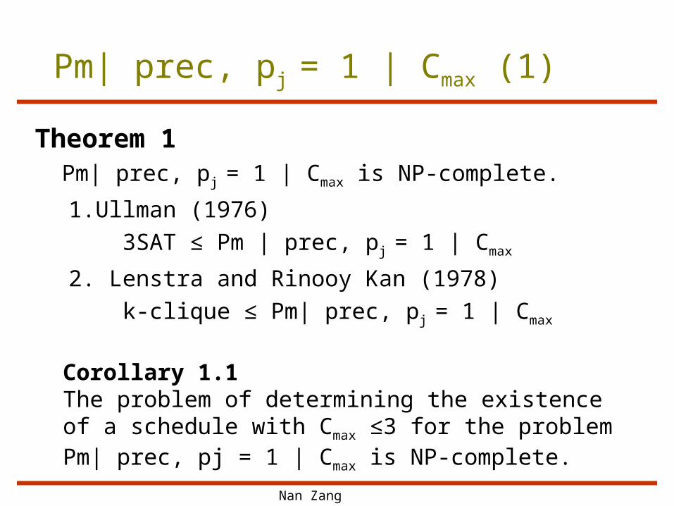
Theorem 1 Pm| prec, pj = 1 | Cmax is NP-complete.
1. Ullman (1976) 3SAT ≤ Pm | prec, pj = 1 | Cmax
2. Lenstra and Rinooy Kan (1978) k-clique ≤ Pm| prec, pj = 1 | Cmax
Corollary 1.1The problem of determining the existence of a schedule with Cmax ≤3 for the problem Pm| prec, pj = 1 | Cmax is NP-complete.

Nan Zang
Pm| prec, pj = 1 | Cmax (2)
Mayr (1985) Theorem 2 Pm | pj =1, SP | Cmax is NP-complete. SP: Series - parallel
Theorem 3 Pm | pj =1, OF | Cmax is NP-complete.
OF: Opposing - forest

Nan Zang
SP and OF
Series-parallel orders Does NOT have a substructure isomorphic to Fig 1. Opposing-forest orders Is a disjoint union of in-tree orders and out-tree orders.
Fig 2: Opposing forest
a
c
b
d
Fig 1

Nan Zang
Conclusion on Pm| prec, pj = 1 | Cmax
3SAT is reducible to the corresponding scheduling problem.
m is a function of the number of clauses in the 3SAT problem.
Results and techniques do not hold for the case Pk | prec, pj = 1 | Cmax

Nan Zang
Classification
Number of processors is a variable (m) Pm | prec, pj = 1 | Cmax
Number of processors is a constant (k) Pk | prec, pj = 1 | Cmax
Nan Zang
Optimal Schedule for Pk | prec, pj = 1 | Cmax
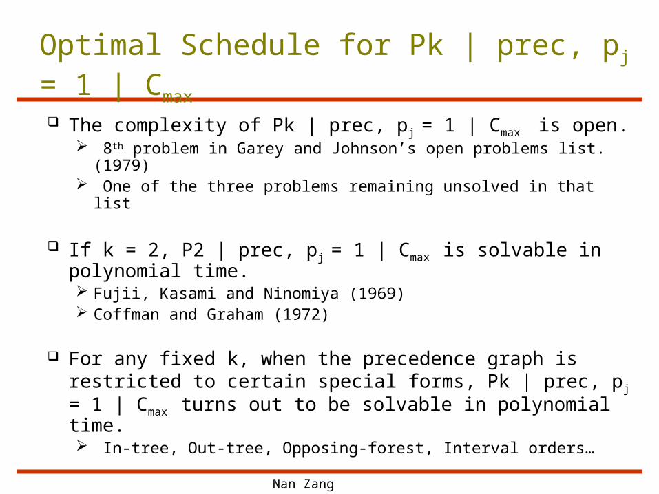
The complexity of Pk | prec, pj = 1 | Cmax is open. 8th problem in Garey and Johnson’s open problems list.
(1979) One of the three problems remaining unsolved in that list
If k = 2, P2 | prec, pj = 1 | Cmax is solvable in polynomial time. Fujii, Kasami and Ninomiya (1969) Coffman and Graham (1972)
For any fixed k, when the precedence graph is restricted to certain special forms, Pk | prec, pj = 1 | Cmax turns out to be solvable in polynomial time. In-tree, Out-tree, Opposing-forest, Interval orders…

Nan Zang
Special precedence constraints In-tree (Out-tree)
In-forest (Out-forest)
Opposing forest
Interval orders
Quasi-interval orders
Over-interval orders
Level orders

Nan Zang
Algorithms for Pk | prec, pj = 1 | Cmax
List scheduling policiesGraham’s list algorithmHLF algorithmMSF algorithmCG algorithm
FKN algorithm (Matching algorithm)
Merge algorithm

Nan Zang
Algorithms for Pk | prec, pj = 1 | Cmax
List scheduling policiesGraham’s list algorithmHLF algorithmMSF algorithmCG algorithm
FKN algorithm (Matching algorithm)
Merge algorithm
Nan Zang
List scheduling policies (1)
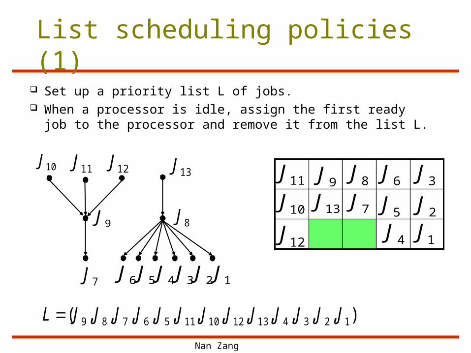
Set up a priority list L of jobs. When a processor is idle, assign the first ready job
to the processor and remove it from the list L.
10J 11J
9J
12J
7J
8J
123456 JJJJJJ
13J
),,,,,,,,,,,,( 12341312101156789 JJJJJJJJJJJJJL
11J
10J
12J
9J
13J8J
7J6J
5J
4J
3J
2J
1J

Nan Zang
Algorithms for Pk | prec, pj = 1 | Cmax
List scheduling policiesGraham’s list algorithmHLF algorithmMSF algorithmCG algorithm
FKN algorithm (Matching algorithm)
Merge algorithm

Nan Zang
Graham’s list algorithm
Graham first analyzed the performance of the simplest list scheduling algorithm.
List scheduling algorithm with an arbitrary job list is called Graham’s list algorithm.
Approximation ratio for Pk | prec, pj = 1 | Cmax
δ = 2-1/k. (Tight!)Approximation ratio is δ if for each input instance, the
makespan produced by the algorithm is at most δ times of the optimal makespan.

Nan Zang
Algorithms for Pk| prec, pj = 1 | Cmax
List scheduling policies
Graham’s list algorithmHLF algorithmMSF algorithmCG algorithm
FKN algorithm (Matching algorithm)
Merge algorithm
Nan Zang
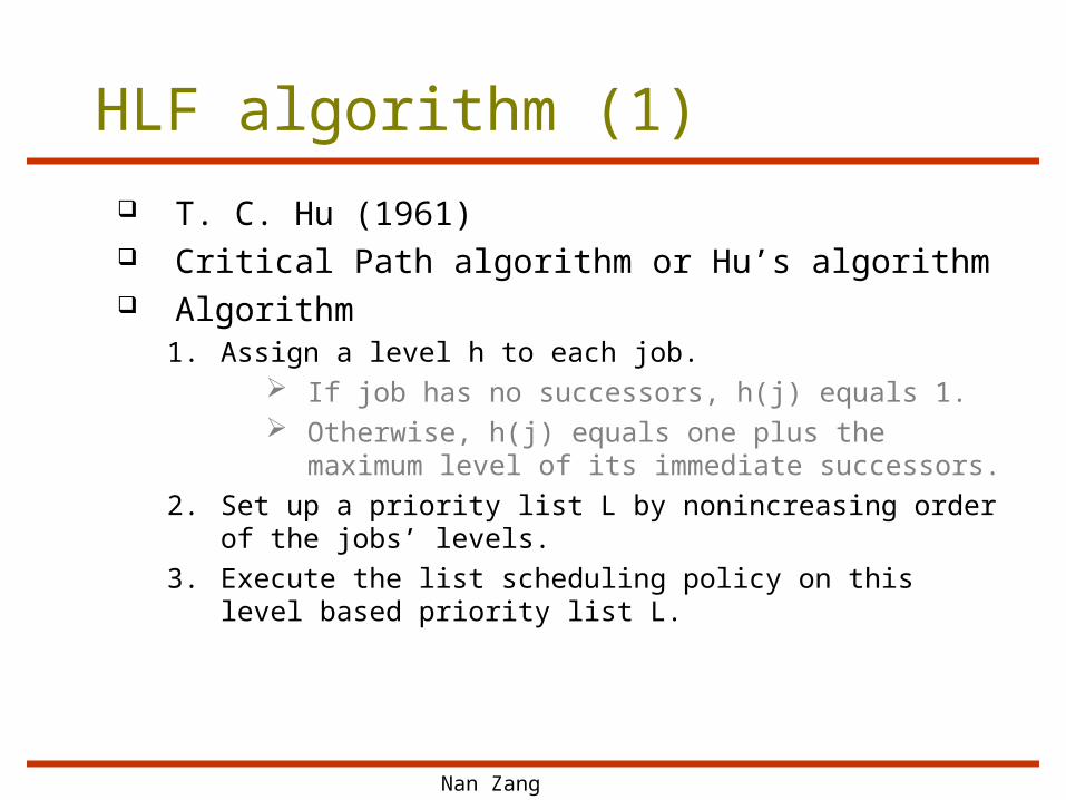
HLF algorithm (1)
T. C. Hu (1961) Critical Path algorithm or Hu’s algorithm Algorithm
1. Assign a level h to each job. If job has no successors, h(j) equals 1. Otherwise, h(j) equals one plus the maximum
level of its immediate successors.2. Set up a priority list L by nonincreasing order of the
jobs’ levels.3. Execute the list scheduling policy on this level
based priority list L.

Nan Zang
HLF algorithm (2)
),,,,,,,,,,,,( 12345678913121110 JJJJJJJJJJJJJL
Level 3 Level 2 Level 1
10J 11J
9J
12J
7J
8J
123456 JJJJJJ
13J
1 1 1 1 1 11
2 2
33 3 310J
11J
12J
13J
9J8J
7J6J
5J
4J
3J
2J
1J
Nan Zang
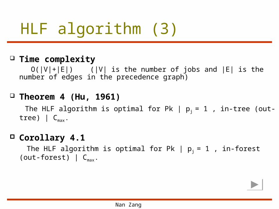
HLF algorithm (3)
Time complexity O(|V|+|E|) (|V| is the number of jobs and |E| is the number of
edges in the precedence graph)
Theorem 4 (Hu, 1961) The HLF algorithm is optimal for Pk | pj = 1 , in-tree (out-tree) | Cmax.
Corollary 4.1 The HLF algorithm is optimal for Pk | pj = 1 , in-forest (out-forest) |
Cmax.
Nan Zang
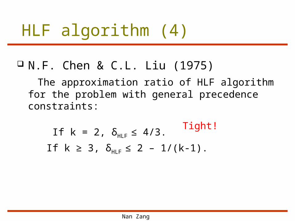
HLF algorithm (4)
N.F. Chen & C.L. Liu (1975) The approximation ratio of HLF algorithm for the
problem with general precedence constraints:
If k = 2, δHLF ≤ 4/3.
If k ≥ 3, δHLF ≤ 2 – 1/(k-1).Tight!

Nan Zang
Algorithms for Pk | prec, pj = 1 | Cmax
List scheduling policies
Graham’s list algorithmHLF algorithmMSF algorithmCG algorithm
FKN algorithm (Matching algorithm)
Merge algorithm

Nan Zang
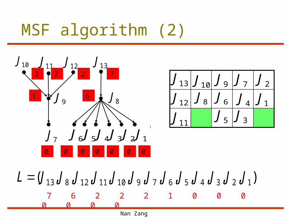
MSF algorithm (1)
Algorithm:Set up a priority list L by nonincreasing order of
the jobs’ successors numbers. (i.e. the job having more successors should have a higher priority in L than the job having fewer successors)
Execute the list scheduling policy based on this priority list L.
Nan Zang
MSF algorithm (2)
),,,,,,,,,,,,( 12345679101112813 JJJJJJJJJJJJJL
10J 11J
9J
12J
7J
8J
123456 JJJJJJ
13J
0 0 0 0 0 00
1 6
72 2 213J
12J
11J
10J
8J9J
6J7J
5J4J
3J
2J
1J
7 6 2 2 2 1 0 0 0 0 0 0 0

Nan Zang
MSF algorithm (3)
Time complexity O(|V|+|E|)
Theorem 5 (Papadimitriou and Yannakakis, 1979)The MSF algorithm is optimal for Pk | pj = 1, interval |
Cmax.
Theorem 6 (Moukrim, 1999)
The MSF algorithm is optimal for Pk | pj = 1, quasi-interval | Cmax.
Nan Zang
Special precedence constraints
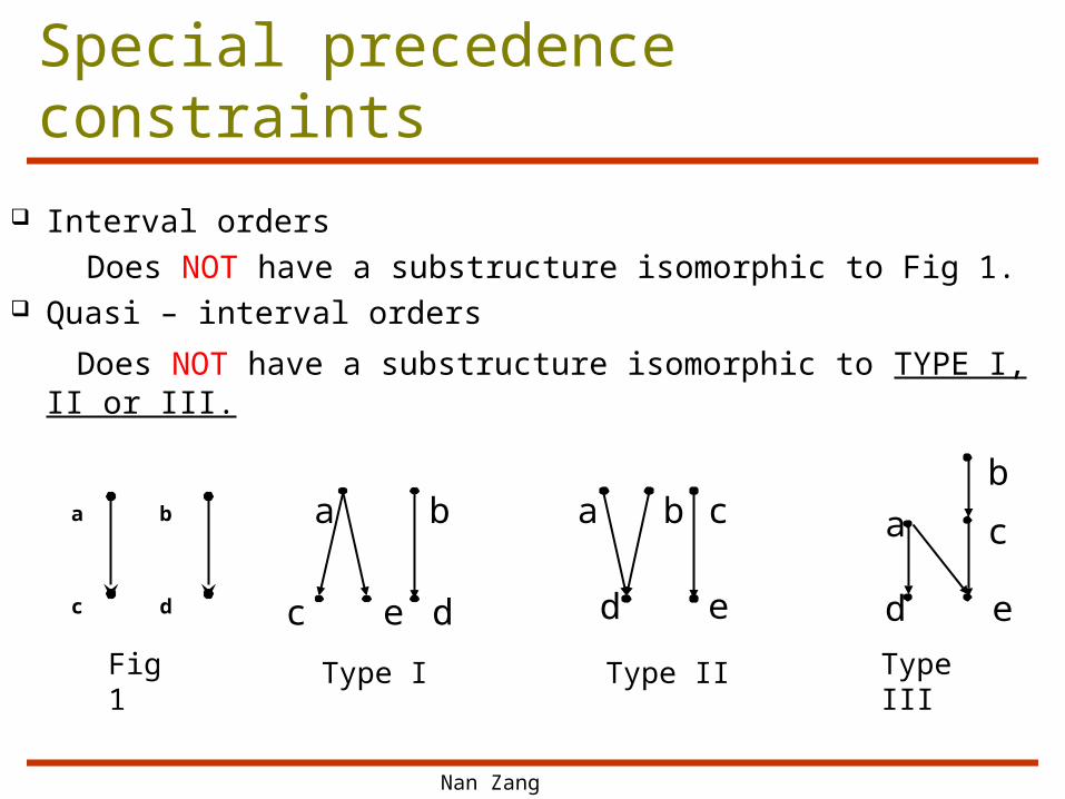
Interval orders Does NOT have a substructure isomorphic to Fig 1. Quasi – interval orders
Does NOT have a substructure isomorphic to TYPE I, II or III.
Type I Type II Type III
e dc
a b
d
ba
e
c
d
b
a
e
ca
c
b
d
Fig 1

Nan Zang
Algorithms for Pk | prec, pj = 1 | Cmax
List scheduling policies
Graham’s list algorithmHLF algorithmMSF algorithmCG algorithm
FKN algorithm (Matching algorithm)
Merge algorithm
Nan Zang
CG algorithm (1)
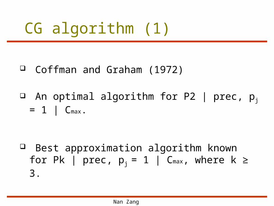
Coffman and Graham (1972)
An optimal algorithm for P2 | prec, pj = 1 | Cmax.
Best approximation algorithm known for Pk | prec, pj = 1 | Cmax, where k ≥ 3.
Nan Zang
Definitions
– Let IS(Jj) denote the immediate successors set of Jj.
– A job is ready to label, if all its immediate successors are labeled and it has not been labeled yet.
– N(Jj) denotes the decreasing sequence of integers formed by ordering of the set { label (Ji) | Ji IS(Jj) }.
– Let label(Jj) be an integer label assigned to Jj.
CG algorithm (2)

Nan Zang
CG algorithm (3)1. Assign a label to each job:
a. Choose an arbitrary task Jk such that IS(Jk) = 0, and define label(Jk) to be 1
b. for i 2 to n do
I. R be the set of jobs that are ready to label.
II. Let J* be the task in R such that N(J*) is lexicographically smaller than N(J) for all J in R
III. Let label(J*) i
end for
2. Construct a list of jobs L = {Jn, Jn-1,…, J2, J1} according to the decreasing order of the labels of the jobs.
3. Execute the list scheduling policy on this priority list L.

Nan Zang
CG algorithm (4)
13J10J 11J
9J
12J
7J
8J
123456 JJJJJJ1 3 4 5 6 72
8 9
1310 11 12
),,,,,,,,,,,,( 76543219810111213 JJJJJJJJJJJJJL
13 12 11 10 9 8 7 6 5 4 3 2 1
)J(IS)J(IS)J(IS
)J(IS)J(IS)J(IS)J(IS
765
4321
}J{)J(IS
}J{)J(IS)J(IS)J(IS
}J{)J(IS
}J,J,J,J,J,J{)J(IS
813
9121110
79
6543218
N(J9)=(1)
N(J8)=(7,6,5,4,3,2)
N(J10)= N(J11)=N(J12)=(8)

Nan Zang
CG algorithm (4)
),,,,,,,,,,,,( 76543219810111213 JJJJJJJJJJJJJL
13J10J 11J
9J
12J
7J
8J
123456 JJJJJJ1 3 4 5 6 72
8 9
1310 11 1213J
12J
11J
10J 9J
1J3J
2J4J
5J
6J
7J
13 12 11 10 9 8 7 6 5 4 3 2 1
8J

Nan Zang
CG algorithm (5)
Time complexity O(|V|+|E|)
Theorem 5 (Coffman and Graham, 1972) The CG algorithm is optimal for P2 | prec, pj = 1| Cmax.
Theorem 6 (Moukrim, 2005) The CG algorithm is optimal for Pk | pj = 1, over-interval |
Cmax.

Nan Zang
Special precedence constraints
Quasi – interval ordersDoes NOT have a substructure isomorphic to TYPE I, II or III.
Over – interval ordersDoes NOT have a substructure isomorphic to TYPE I or II.
Type I Type II Type III
e dc
a b
d
ba
e
c
d
b
a
e
c

Nan Zang
CG algorithm (6)
The performance of CG algorithm when k≥3
Lam and Sethi (1978) δCG ≤ 2 – 2/k
Braschi and Trystram (1994) Cmax(S) ≤ (2 – 2/k) Cmax(S*) – (k – 2 – odd(k))/k (tight!)
Note: S is a CG schedule. S* is an optimal schedule. If k is an odd, odd(k):=1; otherwise, odd(k):=0.

Nan Zang
List Scheduling Policy Conclusions
List scheduling policies
Graham’s list algorithm HLF algorithm MSF algorithm CG algorithm
Property easy to implement extended to the problem Pm | prec, pj = 1|
Cmax
Research directions:
Allow priority lists to depend on the number k of processors.

Nan Zang
Algorithms for Pk | prec, pj = 1 | Cmax
List scheduling policy algorithm
Graham’s list algorithmHLF algorithmMSF algorithmCG algorithm
FKN algorithm (Matching algorithm)
Merge algorithm

Nan Zang
FKN algorithm (1)
Fujii, Kasami and Ninomiya (1969) First optimal algorithm for P2 | prec, pj = 1 | Cmax. Basic Idea
Find a minimum partition of the jobs• There are at most two jobs in each set.• The pair of jobs in the same set can be executed
together. Make a valid schedule according to a particular order
of the partition. (Some clever swap work needed!) The length of the result schedule = value of the min
partition Can be solved by some maximum matching
algorithm.

Nan Zang
FKN algorithm (2) Hard to extend! FKN algorithm cannot be extended to k = 3 directly.
1J2J
3J
4J5J
6J
Minimal partition is {J1, J5, J6} {J4, J2, J3} and |P|=2.
However, The optimal Cmax corresponds partition {J1, J4} {J2,J3,J5} {J6}

Nan Zang
Algorithms for Pk | prec, pj = 1 | Cmax
List scheduling policies
Graham’s list algorithmHLF algorithmMSF algorithmCG algorithm
FKN algorithm (Matching algorithm)
Merge algorithm

Nan Zang
Merge Algorithm (1)
Dolev and Marmuth (1985)
Required input:
An optimal schedule S for a high-graph H(G).
Merge algorithms show how to “ Merge” the known optimal schedule S with the remaining jobs.
Produce an optimal schedule for the whole job set G.

Nan Zang
Merge Algorithm (2)
Definitions height h(G) highest level of the vertices in G.
median μ(G) height of kth highest component +1
high-graph H(G) a subgraph of G, made up of all the components
which are strictly higher than the median. low-graph L(G) remaining subgraph of G, except for H(G)

Nan Zang
Merge Algorithm (3)
C1 C2 C3 C4
H(C1)=5 H(C2)=3 H(C3)=3 H(C4)=2
K=3 3rd highest
μ(G)=4
H(G) L(G)
J3
J2
J10
J4
J5 J6 J7
J1
J9
J12J8
J11
J13
J14
J15
J16

Nan Zang
Merge Algorithm (4)
Idea of the Merge Algorithm If there is an idle period in S, then fill it
with a highest initial vertices in L(G), and remove it from L(G)
Similar to HLF Algorithm

Nan Zang
Merging Algorithm (5)
7J14J11J
10J15J
13J9J
1J 2J 3J 4J 5J
6J
J10
J9
J8
J11
J12
J13
J14
J15
J16
1J 2J 3J 4J 5J
6J8J
12J
16J
7J
S: Optimal schedule for H(G)
L(G)
S’: from merge algorithm

Nan Zang
Merge Algorithm (6)
Theorem 10 (Reduction theorem)
Let G be a precedence graph and S be an optimal schedule for H(G). Then, the Merge algorithm finds an optimal schedule for the whole graph G in time and space O(|V|+|E|).
Corollary 10
If H(G) is empty, then HLF is optimal for G.

Nan Zang
Merge Algorithm (7)
Why Merge algorithm is useful?
1. Find an optimal schedule for a subgraph H(G).
2. H(G) contains fewer than k-1 components.
Precedence Constraints
Time complexity
Level orders O(nk-1)
Opposing forest O(n2k-2logn)
Bounded height O(nh(k-1))
Dolev and Marmuth
How to use it?1. If H(G) is easy to solve.2. If every closed subgraph
of G can be classified into polynomial number of classes.

Nan Zang
Algorithms for Pk | prec, pj = 1 | Cmax
List scheduling policies
Graham’s list algorithmHLF algorithmMSF algorithmCG algorithm
FKN algorithm (Matching algorithm)
Merge algorithm

Nan Zang
Main results known
LIST
Approximation ratio
K=2
K≥3
Intree OFInterval
Quasi-interval
Over-interval
Arbitrary
List 3/2 2-1/k
HLF 4/3 opt 2-1/(k-1)
MSF 4/3 opt opt≥2-1/(k+1)
CG opt opt opt opt opt ≈2-2/k
FKN opt
Merge opt
(Opt: We can get optimal solution in polynomial time. )

Nan Zang
Overview of the paper
Introduction
Classification
Complexity result for Pm | prec, pj = 1 | Cmax
Algorithms for Pk | prec, pj = 1 | Cmax
Future research directions and conclusions

Nan Zang
Future research directions (1)
Finding a new class of orders which can be solved by known algorithms or their generalizations.
over-interval (Moukrim, 2005)
Find an algorithm with a better approximation ratio for the UET scheduling problem.
CG algorithm (1972) Ranade (2003)
special precedence constraints (loosely connected task graphs )
δ = 1.875

Nan Zang
Future research directions (2)
Use the UET multiprocessor scheduling algorithms to solve other related scheduling problems CG algorithm is optimal for P2 | rj, pj = 1| Cmax.
HLF algorithm is optimal for P | rj, pj = 1, outtree| Cmax.
(Huo and Leung, 2005) MSF algorithm is optimal for P | pj = 1, cm=1, quasi-interval| Cmax.
(Moukrim, 2003) CG algorithm is optimal for P2| prmp, pj = 1| Cmax and ∑Cj
(Coffman, Sethuraman and Timkovsky, 2003)
The most challenging research task: Solve the famous open problem Pk |pj = 1| Cmax (k≥3).

Thank You!


