Download - Universal Off-Policy Evaluation

Universal Off-Policy Evaluation
Xuhui Liu
Nanjing University
June 18, 2021
Yash Chandak et al.“Universal Off-Policy Evaluation.” CoRR, 2021.
...
.
...
.
...
.
...
.
...
.
...
.
...
.
...
.
...
.
...
.1/50

Table of Contents
Introduction
Universal Off-Policy Evaluation
High-Confidence Bounds
Experiment Results
Analysis
...
.
...
.
...
.
...
.
...
.
...
.
...
.
...
.
...
.
...
.2/50

Table of Contents
Introduction
Universal Off-Policy Evaluation
High-Confidence Bounds
Experiment Results
Analysis
...
.
...
.
...
.
...
.
...
.
...
.
...
.
...
.
...
.
...
.3/50

Off-Policy Evaluation
Definition: The problem of evaluating a new strategy for behavior, or policy, usingonly observations collected during the execution of another policy.
...
.
...
.
...
.
...
.
...
.
...
.
...
.
...
.
...
.
...
.4/50

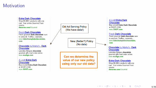
Motivation
Want to evaluate new method without incurring the risk and cost of actuallyimplementing this new method/policy.Existing logs containing huge amounts of historical data based on existing policies.It makes economical sense to, if possible, use these logs.It makes economical sense to, if possible, not risk the loss of testing out a newpotentially bad policy.Online ad placement is a good example.
...
.
...
.
...
.
...
.
...
.
...
.
...
.
...
.
...
.
...
.5/50
Motivation
...
.
...
.
...
.
...
.
...
.
...
.
...
.
...
.
...
.
...
.6/50
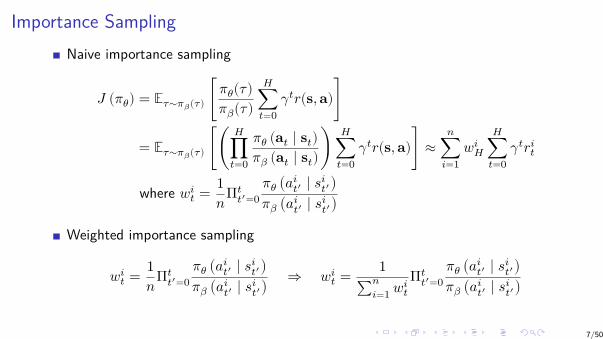
Importance SamplingNaive importance sampling
𝐽 (𝜋𝜃) = 𝔼𝜏∼𝜋𝛽(𝜏) [ 𝜋𝜃(𝜏)𝜋𝛽(𝜏)
𝐻∑𝑡=0
𝛾𝑡𝑟(s, a)]
= 𝔼𝜏∼𝜋𝛽(𝜏) [(𝐻
∏𝑡=0
𝜋𝜃 (a𝑡 ∣ s𝑡)𝜋𝛽 (a𝑡 ∣ s𝑡)
)𝐻
∑𝑡=0
𝛾𝑡𝑟(s, a)] ≈𝑛
∑𝑖=1
𝑤𝑖𝐻
𝐻∑𝑡=0
𝛾𝑡𝑟𝑖𝑡
where 𝑤𝑖𝑡 = 1
𝑛Π𝑡𝑡′=0
𝜋𝜃 (𝑎𝑖𝑡′ ∣ 𝑠𝑖
𝑡′)𝜋𝛽 (𝑎𝑖
𝑡′ ∣ 𝑠𝑖𝑡′)
Weighted importance sampling
𝑤𝑖𝑡 = 1
𝑛Π𝑡𝑡′=0
𝜋𝜃 (𝑎𝑖𝑡′ ∣ 𝑠𝑖
𝑡′)𝜋𝛽 (𝑎𝑖
𝑡′ ∣ 𝑠𝑖𝑡′)
⇒ 𝑤𝑖𝑡 = 1
∑𝑛𝑖=1 𝑤𝑖
𝑡Π𝑡
𝑡′=0𝜋𝜃 (𝑎𝑖
𝑡′ ∣ 𝑠𝑖𝑡′)
𝜋𝛽 (𝑎𝑖𝑡′ ∣ 𝑠𝑖
𝑡′)
...
.
...
.
...
.
...
.
...
.
...
.
...
.
...
.
...
.
...
.7/50

Statistical Quantities
Consider a random variable 𝑋, the cumulative distribution function and probabilitydistribution function of which are 𝐹(𝑥) and 𝑝(𝑥), respectively.
Mean 𝔼[𝑋].Quantile quantile𝛼(𝑋) = 𝐹 −1(𝛼).Value at Risk (VaR) VaR𝛼(𝑋) = quantile𝛼.Conditional Value at Risk (CVaR) CVaR𝛼(𝑋) = 𝔼[𝑋|𝑋 ≤ quantile𝛼(𝑋)].Variance 𝔼[(𝑋 − 𝔼𝑋)2].Entropy 𝐻(𝑋) = ∫ 𝑝(𝑥) log 𝑝(𝑥)𝑑𝑥.
...
.
...
.
...
.
...
.
...
.
...
.
...
.
...
.
...
.
...
.8/50

Illustration
...
.
...
.
...
.
...
.
...
.
...
.
...
.
...
.
...
.
...
.9/50

Limitations
Safety critical applications, e.g., automated healthcare.Risk-prone metrics: Value at risk (VaR) and conditional value at risk(CVaR).
Applications like online recommendations are subject to noisy dataRobust metrics: Median and other quantiles.
Applications involving direct human-machine interaction, such as robotics andautonomous driving.Uncertainty metrics: Variance and entropy.
...
.
...
.
...
.
...
.
...
.
...
.
...
.
...
.
...
.
...
.10/50

How do we develop a universal off-policy method—one that can estimate any desiredperformance metrics and can also provide high-confidence bounds that holdsimultaneously with high probability for those metrics?
...
.
...
.
...
.
...
.
...
.
...
.
...
.
...
.
...
.
...
.11/50

Table of Contents
Introduction
Universal Off-Policy Evaluation
High-Confidence Bounds
Experiment Results
Analysis
...
.
...
.
...
.
...
.
...
.
...
.
...
.
...
.
...
.
...
.12/50
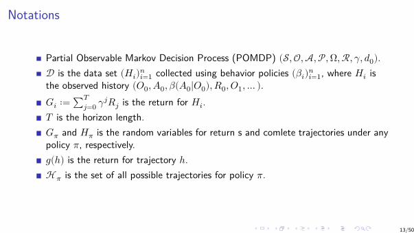
Notations
Partial Observable Markov Decision Process (POMDP) (𝒮, 𝒪, 𝒜, 𝒫, Ω, ℛ, 𝛾, 𝑑0).𝒟 is the data set (𝐻𝑖)𝑛
𝑖=1 collected using behavior policies (𝛽𝑖)𝑛𝑖=1, where 𝐻𝑖 is
the observed history (𝑂0, 𝐴0, 𝛽(𝐴0|𝑂0), 𝑅0, 𝑂1, … ).𝐺𝑖 ∶= ∑𝑇
𝑗=0 𝛾𝑗𝑅𝑗 is the return for 𝐻𝑖.𝑇 is the horizon length.𝐺𝜋 and 𝐻𝜋 is the random variables for return s and comlete trajectories under anypolicy 𝜋, respectively.𝑔(ℎ) is the return for trajectory ℎ.ℋ𝜋 is the set of all possible trajectories for policy 𝜋.
...
.
...
.
...
.
...
.
...
.
...
.
...
.
...
.
...
.
...
.13/50

Assumptions
Assumption 1The set 𝒟 contains independent (not necessarily identically distributed) historiesgenerated using (𝛽𝑖)𝑛
𝑖=1, along with the probability of the actions chosen, such that forsome 𝜖 > 0, (𝛽𝑖(𝑎|𝑜) < 𝜖) ⟹ (𝜋(𝑎|𝑜) = 0), for all 𝑜 ∈ 𝒪, 𝑎 ∈ 𝒜, and 𝑖 ∈ (1, … , 𝑛).
...
.
...
.
...
.
...
.
...
.
...
.
...
.
...
.
...
.
...
.14/50
Method
First estimate its cumulative distribution 𝐹𝜋.Then use it to estimate its parameter 𝜓(𝐹𝜋).
...
.
...
.
...
.
...
.
...
.
...
.
...
.
...
.
...
.
...
.15/50

Method
Represent 𝐹𝜋 with return 𝐺𝜋.
𝐹𝜋(𝜈) = Pr (𝐺𝜋 ≤ 𝜈) = ∑𝑥∈𝒳,𝑥≤𝜈
Pr (𝐺𝜋 = 𝑥) = ∑𝑥∈𝒳,𝑥≤𝜈
( ∑ℎ∈ℋ𝜋
Pr (𝐻𝜋 = ℎ) 𝟙{𝑔(ℎ)=𝑥})
Exchange the order of Sum.
𝐹𝜋(𝜈) = ∑ℎ∈ℋ𝜋
Pr (𝐻𝜋 = ℎ) ∑𝑥∈𝒳,𝑥≤𝜈
𝟙{𝑔(ℎ)=𝑥} = ∑ℎ∈ℋ𝜋
Pr (𝐻𝜋 = ℎ) (𝟙{𝑔(ℎ)≤𝜈})
...
.
...
.
...
.
...
.
...
.
...
.
...
.
...
.
...
.
...
.16/50
Method
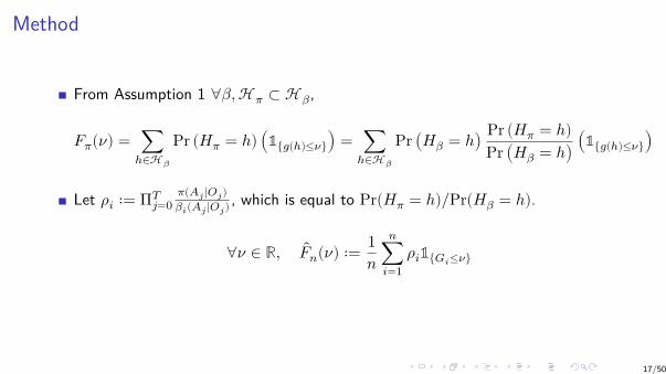
From Assumption 1 ∀𝛽, ℋ𝜋 ⊂ ℋ𝛽,
𝐹𝜋(𝜈) = ∑ℎ∈ℋ𝛽
Pr (𝐻𝜋 = ℎ) (𝟙{𝑔(ℎ)≤𝜈}) = ∑ℎ∈ℋ𝛽
Pr (𝐻𝛽 = ℎ) Pr (𝐻𝜋 = ℎ)Pr (𝐻𝛽 = ℎ) (𝟙{𝑔(ℎ)≤𝜈})
Let 𝜌𝑖 ∶= Π𝑇𝑗=0
𝜋(𝐴𝑗|𝑂𝑗)𝛽𝑖(𝐴𝑗|𝑂𝑗) , which is equal to Pr(𝐻𝜋 = ℎ)/Pr(𝐻𝛽 = ℎ).
∀𝜈 ∈ ℝ, 𝐹𝑛(𝜈) ∶= 1𝑛
𝑛∑𝑖=1
𝜌𝑖𝟙{𝐺𝑖≤𝜈}
...
.
...
.
...
.
...
.
...
.
...
.
...
.
...
.
...
.
...
.17/50

Illustration
...
.
...
.
...
.
...
.
...
.
...
.
...
.
...
.
...
.
...
.18/50

Partial Observable Setting
𝒪, 𝒪: Observation set for the behavior policy and the evaluation policy.If 𝒪 = 𝒪 = 𝒮, it becomes MDP setting.If 𝒪 = 𝒪, as 𝛽(𝑎|𝑜) = 𝛽(𝑎| 𝑜), one can use density estimation on the availabledata, 𝒟, to construct an estimator 𝛽(𝑎|𝑜) of Pr(𝑎| 𝑜) = 𝛽(𝑎| 𝑜).
𝒪 ≠ 𝒪, it is only possible to estimate Pr(𝑎| 𝑜) = ∑𝑥∈𝑜 𝛽(𝑎|𝑥)Pr(𝑥| 𝑜) throughdensity estimation using data 𝒟.
...
.
...
.
...
.
...
.
...
.
...
.
...
.
...
.
...
.
...
.19/50

Probability Distribution and Inverse CDF
Let (𝐺(𝑖))𝑛𝑖=1 be the order statistics for samples (𝐺𝑖)𝑛
𝑖=1 and 𝐺0 ∶= 𝐺min.
Inverse CDF𝐹 −1𝑛 (𝛼) ∶= min {𝑔 ∈ (𝐺(𝑖))
𝑛𝑖=1
∣ 𝐹𝑛(𝑔) ≥ 𝛼}
Probability distributiond 𝐹𝑛 (𝐺(𝑖)) ∶= 𝐹𝑛 (𝐺(𝑖)) − 𝐹𝑛 (𝐺(𝑖−1))
...
.
...
.
...
.
...
.
...
.
...
.
...
.
...
.
...
.
...
.20/50

Estimator
𝜇𝜋 ( 𝐹𝑛) ∶= ∑𝑛𝑖=1 d 𝐹𝑛 (𝐺(𝑖)) 𝐺(𝑖),
𝜎2𝜋 ( 𝐹𝑛) ∶= ∑𝑛
𝑖=1 d 𝐹𝑛 (𝐺(𝑖)) (𝐺(𝑖) − 𝜇𝜋 ( 𝐹𝑛))2 ,𝑄𝛼
𝜋 ( 𝐹𝑛) ∶= 𝐹 −1𝑛 (𝛼),
CVaR𝛼𝜋 ( 𝐹𝑛) ∶= 1
𝛼 ∑𝑛𝑖=1 d 𝐹𝑛 (𝐺(𝑖)) 𝐺(𝑖)𝟙{𝐺(𝑖)≤𝑄𝛼𝜋 ( 𝐹𝑛) } .
• Definition of CVaR:CVaR𝛼
𝜋 (𝐹𝜋) = 𝔼 [𝐺𝜋 ∣ 𝐺𝜋 ≤ 𝐹 −1𝜋 (𝛼)]
...
.
...
.
...
.
...
.
...
.
...
.
...
.
...
.
...
.
...
.21/50

Table of Contents
Introduction
Universal Off-Policy Evaluation
High-Confidence Bounds
Experiment Results
Analysis
...
.
...
.
...
.
...
.
...
.
...
.
...
.
...
.
...
.
...
.22/50
High-Confidence Bounds
1. It’s easy to obtain bounds for a single point.2. It’s hard hard to obtain bounds for a interval.3. CDF is monotonically non-decreasing.
Let (𝜅𝑖)𝐾𝑖=1 be any K “key points at which we obtain confidence interval for
(𝐹𝜋(𝜅𝑖))𝐾𝑖=1.
Generalize to whole interval based on these “key points”.
...
.
...
.
...
.
...
.
...
.
...
.
...
.
...
.
...
.
...
.23/50

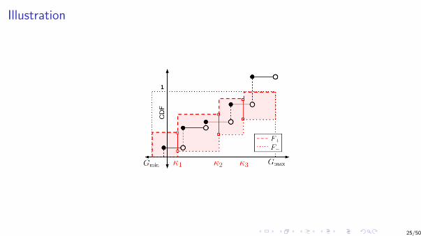
Let CI− (𝜅𝑖, 𝛿𝑖) and CI+ (𝜅𝑖, 𝛿𝑖) be the lower and the upper confidence bounds on𝐹𝜋 (𝜅𝑖), respectively, such that
∀𝑖 ∈ (1, … , 𝐾), Pr (CI− (𝜅𝑖, 𝛿𝑖) ≤ 𝐹𝜋 (𝜅𝑖) ≤ CI+ (𝜅𝑖, 𝛿𝑖)) ≥ 1 − 𝛿𝑖
Based on this constuction, we formulate a lower function 𝐹− and an upper function 𝐹+:
𝐹−(𝜈) ∶= { 1 if 𝜈 > 𝐺maxmax𝜅𝑖≤𝜈 𝐶𝐼− (𝜅𝑖, 𝛿𝑖) otherwise
𝐹+(𝜈) ∶= { 0 if 𝜈 < 𝐺minmin𝜅𝑖≥𝜈 𝐶𝐼+ (𝜅𝑖, 𝛿𝑖) otherwise
...
.
...
.
...
.
...
.
...
.
...
.
...
.
...
.
...
.
...
.24/50
Illustration
...
.
...
.
...
.
...
.
...
.
...
.
...
.
...
.
...
.
...
.25/50

Illustration
...
.
...
.
...
.
...
.
...
.
...
.
...
.
...
.
...
.
...
.26/50

Illustration
...
.
...
.
...
.
...
.
...
.
...
.
...
.
...
.
...
.
...
.27/50

Bootstrap Bounds1
1B. Efron and R. J. Tibshirani. “An introduction to the Bootstrap”. CRC press, 1994..
.
...
..
.
...
.
...
.
...
.
...
.
...
.
...
.
...
.
...
.28/50

Non-stationary
Assumption 3For any 𝜈, ∃𝑤𝜈 ∈ ℝ𝑑, such that, ∀𝑖 ∈ [1, 𝐿 + ℓ], 𝐹 (𝑖)
𝜋 (𝜈) = 𝜙(𝑖)⊤𝑤𝜈.
Estimating 𝐹 (𝑖)𝜋 can now be seen as a time-series forecasting problem.
Wild bootstrap2 provides approximate CIs.
2E. Mammen. “Bootstrap and wild bootstrap for high dimensional linear models.” The Annals ofStatistics, pages 255–285, 1993.
...
.
...
.
...
.
...
.
...
.
...
.
...
.
...
.
...
.
...
.29/50

Table of Contents
Introduction
Universal Off-Policy Evaluation
High-Confidence Bounds
Experiment Results
Analysis
...
.
...
.
...
.
...
.
...
.
...
.
...
.
...
.
...
.
...
.30/50

Setting
A simulated stationary and a non-stationary recommender system domain,where the user’s interest for a finite set of items is represented using thecorresponding item’s reward.Type-1 Diabetes Mellitus Simulator (T1DMS) for the treatment of type-1diabetes.A continuous-state Gridworld with partial observability (which also makes thedomain non-Markovian in the observations), stochastic transitions, and eightdiscrete actions corresponding to up, down, left, right, and the four diagonalmovements.
...
.
...
.
...
.
...
.
...
.
...
.
...
.
...
.
...
.
...
.31/50
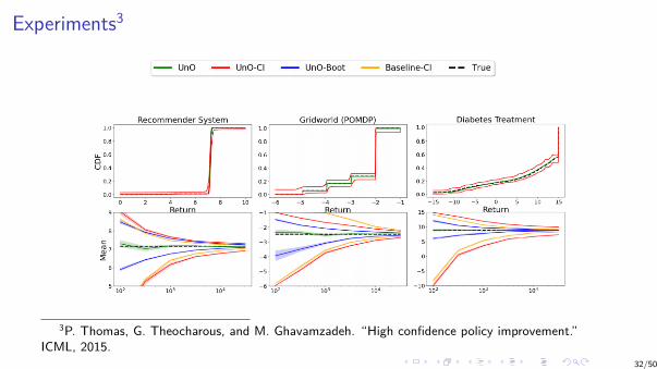
Experiments3
3P. Thomas, G. Theocharous, and M. Ghavamzadeh. “High confidence policy improvement.”ICML, 2015.
...
.
...
.
...
.
...
.
...
.
...
.
...
.
...
.
...
.
...
.32/50

Experiments4
4Y. Chandak, S. Shankar, and P. S. Thomas. “High confidence off-policy (or counterfactual)variance estimation.” AAAI, 2021.
...
.
...
.
...
.
...
.
...
.
...
.
...
.
...
.
...
.
...
.33/50

...
.
...
.
...
.
...
.
...
.
...
.
...
.
...
.
...
.
...
.34/50

Table of Contents
Introduction
Universal Off-Policy Evaluation
High-Confidence Bounds
Experiment Results
Analysis
...
.
...
.
...
.
...
.
...
.
...
.
...
.
...
.
...
.
...
.35/50

Theorem
Estimator∀𝜈 ∈ ℝ, 𝐹𝑛(𝜈) ∶= 1
𝑛𝑛
∑𝑖=1
𝜌𝑖𝟙{𝐺𝑖≤𝜈}
Theoretical guarantee
...
.
...
.
...
.
...
.
...
.
...
.
...
.
...
.
...
.
...
.36/50

Part 1 UnbiasednessRecall that
𝐹𝜋(𝜈) = ∑ℎ∈ℋ𝛽
Pr (𝐻𝜋 = ℎ) (𝟙{𝑔(ℎ)≤𝜈}) = ∑ℎ∈ℋ𝛽
Pr (𝐻𝛽 = ℎ) Pr (𝐻𝜋 = ℎ)Pr (𝐻𝛽 = ℎ) (𝟙{𝑔(ℎ)≤𝜈})
The probability of a trajectory under a policy 𝜋 with partial observations andnon-Markovian structure is
Pr (𝐻𝜋 = ℎ) = Pr (𝑠0) Pr (𝑜0 ∣ 𝑠0) Pr ( 𝑜0 ∣ 𝑜0, 𝑠0) Pr (𝑎0 ∣ 𝑠0, 𝑜0, 𝑜0; 𝜋)
×𝑇 −1∏𝑖=0
(Pr (𝑟𝑖 ∣ ℎ𝑖) Pr (𝑠𝑖+1 ∣ ℎ𝑖) Pr (𝑜𝑖+1 ∣ 𝑠𝑖+1, ℎ𝑖) Pr ( 𝑜𝑖+1 ∣ 𝑠𝑖+1, 𝑜𝑖+1, ℎ𝑖)
× Pr (𝑎𝑖+1 ∣ 𝑠𝑖+1, 𝑜𝑖+1, 𝑜𝑖+1, ℎ𝑖; 𝜋)) Pr (𝑟𝑇 ∣ ℎ𝑇 )
...
.
...
.
...
.
...
.
...
.
...
.
...
.
...
.
...
.
...
.37/50

The ratio can be written as
Pr (𝐻𝜋 = ℎ)Pr (𝐻𝛽 = ℎ) = Pr (𝑎0 ∣ 𝑠0, 𝑜0, 𝑜0; 𝜋)
Pr (𝑎0 ∣ 𝑠0, 𝑜0, 𝑜0; 𝛽)𝑇 −1∏𝑖=0
Pr (𝑎𝑖+1 ∣ 𝑠𝑖+1, 𝑜𝑖+1, 𝑜𝑖+1, ℎ𝑖; 𝜋)Pr (𝑎𝑖+1 ∣ 𝑠𝑖+1, 𝑜𝑖+1, 𝑜𝑖+1, ℎ𝑖; 𝛽)
=𝑇
∏𝑖=0
𝜋 (𝑎𝑖 ∣ 𝑜𝑖)𝛽 (𝑎𝑖 ∣ 𝑜𝑖)
= 𝜌(ℎ)
Then we have𝐹𝜋(𝜈) = ∑
ℎ∈ℋ𝛽
Pr(𝐻𝛽 = ℎ)𝜌(ℎ)(𝟙{𝑔(ℎ)≤𝜈}).
...
.
...
.
...
.
...
.
...
.
...
.
...
.
...
.
...
.
...
.38/50

𝔼𝒟 [ 𝐹𝑛(𝜈)] = 𝔼𝒟 [ 1𝑛
𝑛∑𝑖=1
𝜌𝑖 (𝟙{𝐺𝑖≤𝜈})]
= 1𝑛
𝑛∑𝑖=1
𝔼𝒟 [𝜌𝑖 (𝟙{𝐺𝑖≤𝜈})]
= 1𝑛
𝑛∑𝑖=1
∑ℎ∈ℋ𝛽𝑖
Pr (𝐻𝛽𝑖= ℎ) 𝜌(ℎ) (𝟙{𝑔(ℎ)≤𝜈})
(𝑎)= 1𝑛
𝑛∑𝑖=1
𝐹𝜋(𝜈)
= 𝐹𝜋(𝜈)
...
.
...
.
...
.
...
.
...
.
...
.
...
.
...
.
...
.
...
.39/50

Part 2 Uniform Consistency
First we show pointwise consistency, i.e., for all 𝜈, 𝐹𝑛(𝜈) a.s.⟶ 𝐹𝜋(𝜈).
Then we use this to establish uniform consistency.
...
.
...
.
...
.
...
.
...
.
...
.
...
.
...
.
...
.
...
.40/50
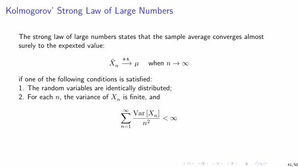
Kolmogorov’ Strong Law of Large Numbers
The strong law of large numbers states that the sample average converges almostsurely to the expexted value:
��𝑛a.s.⟶ 𝜇 when 𝑛 → ∞
if one of the following conditions is satisfied:1. The random variables are identically distributed;2. For each 𝑛, the variance of 𝑋𝑛 is finite, and
∞∑𝑛=1
Var [𝑋𝑛]𝑛2 < ∞
...
.
...
.
...
.
...
.
...
.
...
.
...
.
...
.
...
.
...
.41/50
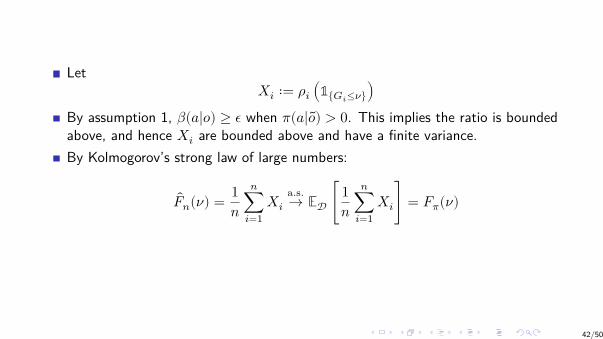
Let𝑋𝑖 ∶= 𝜌𝑖 (𝟙{𝐺𝑖≤𝜈})
By assumption 1, 𝛽(𝑎|𝑜) ≥ 𝜖 when 𝜋(𝑎| 𝑜) > 0. This implies the ratio is boundedabove, and hence 𝑋𝑖 are bounded above and have a finite variance.By Kolmogorov’s strong law of large numbers:
𝐹𝑛(𝜈) = 1𝑛
𝑛∑𝑖=1
𝑋𝑖a.s.→ 𝔼𝒟 [ 1
𝑛𝑛
∑𝑖=1
𝑋𝑖] = 𝐹𝜋(𝜈)
...
.
...
.
...
.
...
.
...
.
...
.
...
.
...
.
...
.
...
.42/50

Some extra notation to tackle discontinuities in CDF 𝐹𝜋
𝐹𝜋 (𝜈−) ∶= Pr (𝐺𝜋 < 𝜈) = 𝐹𝜋(𝜈) − Pr (𝐹𝜋 = 𝜈) , 𝐹𝑛 (𝜈−) ∶= 1𝑛
𝑛∑𝑖=1
𝜌𝑖 (𝟙{𝐺𝑖<𝜈})
Similarly, we have𝐹𝑛 (𝜈−) a.s⟶ 𝐹𝜋 (𝜈−)
...
.
...
.
...
.
...
.
...
.
...
.
...
.
...
.
...
.
...
.43/50

Let 𝜖1 > 0, and let 𝐾 be any value more than 1/𝜖1. Let (𝜅𝑖)𝐾𝑖=0 be 𝐾 key points,
𝐺min = 𝜅0 < 𝜅1 ≤ 𝜅2 … ≤ 𝜅𝐾−1 < 𝜅𝐾 = 𝐺max
which create 𝐾 intervals such that for all 𝑖 ∈ (1, … , 𝐾 − 1),
𝐹𝜋 (𝜅−𝑖 ) ≤ 𝑖
𝐾 ≤ 𝐹𝜋 (𝜅𝑖)
Then by construction, if 𝜅𝑖−1 < 𝜅𝑖,
𝐹𝜋 (𝜅−𝑖 ) − 𝐹𝜋 (𝜅𝑖−1) ≤ 𝑖
𝐾 − 𝑖 − 1𝐾 = 1
𝐾 < 𝜖1.
...
.
...
.
...
.
...
.
...
.
...
.
...
.
...
.
...
.
...
.44/50

For any 𝜈, let 𝜅𝑖−1 and 𝜅𝑖 be such that 𝜅𝑖−1 ≤ 𝜈 < 𝜅𝑖. Then,
𝐹𝑛(𝜈) − 𝐹𝜋(𝜈) ≤ 𝐹𝑛 (𝜅−𝑖 ) − 𝐹𝜋 (𝜅𝑖−1)
≤ 𝐹𝑛 (𝜅−𝑖 ) − 𝐹𝜋 (𝜅−
𝑖 ) + 𝜖1.
Similarly,𝐹𝑛(𝜈) − 𝐹𝜋(𝜈) ≥ 𝐹𝑛 (𝜅𝑖−1) − 𝐹𝜋 (𝜅−
𝑖 )≥ 𝐹𝑛 (𝜅𝑖−1) − 𝐹𝜋 (𝜅𝑖−1) − 𝜖1
...
.
...
.
...
.
...
.
...
.
...
.
...
.
...
.
...
.
...
.45/50

Then, ∀𝜈 ∈ ℝ,
𝐹𝑛 (𝜅𝑖−1) − 𝐹𝜋 (𝜅𝑖−1) − 𝜖1 ≤ 𝐹𝑛(𝜈) − 𝐹𝜋(𝜈) ≤ 𝐹𝑛 (𝜅−𝑖 ) − 𝐹𝜋 (𝜅−
𝑖 ) + 𝜖1,
LetΔ𝑛 ∶= max
𝑖∈(1…𝐾−1){∣ 𝐹𝑛 (𝜅𝑖) − 𝐹𝜋 (𝜅𝑖)∣ , ∣ 𝐹𝑛 (𝜅−
𝑖 ) − 𝐹𝜋 (𝜅−𝑖 )∣}
By the pointwise convergence, we have
Δ𝑛a.s.→ 0
and thus,∣ 𝐹𝑛(𝜈) − 𝐹𝜋(𝜈)∣ ≤ Δ𝑛 + 𝜖1
Finally, since the inequality holds for ∀𝜈 ∈ ℝ and is valid for any 𝜖1 > 0, making𝜖1 → 0 gives the desired result,
sup𝜈∈ℝ
∣ 𝐹𝑛(𝜈) − 𝐹𝜋(𝜈)∣ a.s.⟶ 0
...
.
...
.
...
.
...
.
...
.
...
.
...
.
...
.
...
.
...
.46/50

Variance Reduction
Inspired by weighted importance sampling
∀𝜈 ∈ ℝ, 𝐹𝑛(𝜈) ∶= 1∑𝑛
𝑗=1 𝜌𝑗(
𝑛∑𝑖=1
𝜌𝑖 (𝟙{𝐺𝑖≤𝜈})) .
Under Assumption 1, 𝐹𝑛 may be biased but is a uniformly consistent estimator of𝐹𝜋,
∀𝜈 ∈ ℝ, 𝔼𝒟 [ 𝐹𝑛(𝜈)] ≠ 𝐹𝜋, sup𝜈∈ℝ
∣ 𝐹𝑛(𝜈) − 𝐹𝜋(𝜈)∣ a.s.⟶ 0
...
.
...
.
...
.
...
.
...
.
...
.
...
.
...
.
...
.
...
.47/50

Part 1 Biased: We prove this using a counter-example. Let 𝑛 = 1, so
∀𝜈 ∈ ℝ, 𝔼𝒟 [ 𝐹𝑛(𝜈)] = 𝔼𝒟 ⎡⎢⎣
1∑1
𝑗=1 𝜌𝑗(
1∑𝑖=1
𝜌𝑖𝟙{𝐺𝑖≤𝜈})⎤⎥⎦
= 𝔼𝒟 [𝟙{𝐺1≤𝜈}](𝑎)= ∑
ℎ∈ℋ𝛽1
Pr (𝐻𝛽1= ℎ) (𝟙{𝑔(ℎ)≤𝜈})
= 𝐹𝛽1(𝜈)
≠ 𝐹𝜋(𝜈)
...
.
...
.
...
.
...
.
...
.
...
.
...
.
...
.
...
.
...
.48/50
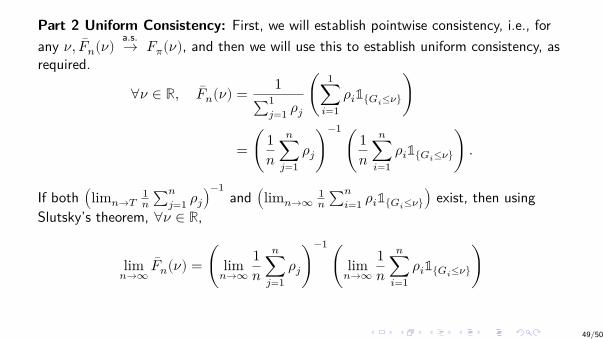
Part 2 Uniform Consistency: First, we will establish pointwise consistency, i.e., forany 𝜈, 𝐹𝑛(𝜈) a.s.→ 𝐹𝜋(𝜈), and then we will use this to establish uniform consistency, asrequired.
∀𝜈 ∈ ℝ, 𝐹𝑛(𝜈) = 1∑1
𝑗=1 𝜌𝑗(
1∑𝑖=1
𝜌𝑖𝟙{𝐺𝑖≤𝜈})
= ( 1𝑛
𝑛∑𝑗=1
𝜌𝑗)−1
( 1𝑛
𝑛∑𝑖=1
𝜌𝑖𝟙{𝐺𝑖≤𝜈}) .
If both (lim𝑛→𝑇1𝑛 ∑𝑛
𝑗=1 𝜌𝑗)−1
and (lim𝑛→∞1𝑛 ∑𝑛
𝑖=1 𝜌𝑖𝟙{𝐺𝑖≤𝜈}) exist, then usingSlutsky’s theorem, ∀𝜈 ∈ ℝ,
lim𝑛→∞
𝐹𝑛(𝜈) = ( lim𝑛→∞
1𝑛
𝑛∑𝑗=1
𝜌𝑗)−1
( lim𝑛→∞
1𝑛
𝑛∑𝑖=1
𝜌𝑖𝟙{𝐺𝑖≤𝜈})
...
.
...
.
...
.
...
.
...
.
...
.
...
.
...
.
...
.
...
.49/50

Notice using Kolmogorov’s strong law of large numbers that the term in the firstparentheses will converge to the expected value of importance ratios, which equals one.Similarly, we know that the term in the second parentheses will converge to 𝐹𝜋(𝜈)almost surely. Therefore,
∀𝜈 ∈ ℝ, 𝐹𝑛(𝜈) a.s.⟶ (1)−1 (𝐹𝜋(𝜈)) = 𝐹𝜋(𝜈)
...
.
...
.
...
.
...
.
...
.
...
.
...
.
...
.
...
.
...
.50/50


