
·\
ANALYSIS OF HYDROLOGIC SYSTEMS
by
Tsung-Ting Chiang, B.S., M.S. # • ,
Thesis submitted to the Graduate Faculty of the
Virginia Polytechnic Institute
in partial fulfillment for the degree of
DOCTOR OF PHILOSOPHY
in
Civil ineering
APPROVED:
./
~JJt, ~ ch1n '1J7CH-~ Dr. R. M. Barker Dr. H. M. Morris
January, 1968
Blacksburg, Virginia
. \

LD 5bSS V850 } 908 C45 G'~

TABLE OF CONTENTS
Page
I. INTRODUCTION .•.•.. · . . . . . . . . . 1
II. REVIEW OF THE LITERATURE. 4
III.
IV.
V.
VII.
LABORATORY EQUIPMENT • • · . . . . • 10
Water Supply • • •• • • • • • • • 10 Rainfall Simulator • • • • ••• • • • 10 Ca tchmen t •• • •• ••••. •••• 12 Outflow Measurement. • • • • • • • • • 14 Measurement of Discharge • • • • • • • • . • • 14 Measurement of Slope • • .• • • • 14
THEORETICAL CONSIDERATtONS • · . . . • 16
Similarity Considerations •.••••••••• 17 Dynamic Analysis . • . . • • • • • • • • • . • 18 Terminology • • • • • • • . • • • • • 20 Theoretical Analysis .•• . • • • 25
RESULT~. • . . . . . . . . . . . . . . • 30 "
• 30 • 36
Delay or Dead Time, Td • • • • •. • •• Response . . • • • •• • • • • • • • Bode Diagrams •••• • • • Time Constant and Damping Coefficient.
• 44 . • 56
Nonlinear Parameter. . • • . • • . Transfer Function • . . • • . Digital-Analog Simulation ••• Application to Natural Basins.
• • • • 59
DISCUSSION • . . . . · . . . CONCLUSION • • . . . . .
• • • '* • • 62
· . . . · . . .
· 65 66
• • 78
• 83
VIII. GLOSSARY ••. . . . . . . . . . . · 85
IX. ACKNOWLEDGHENTS .. · 87
x. BIBLIOGRAPHY • . 88
XI. VITA • • • • • · • 95
ii

XII ..
Page
APPENDICES .. .. 96
A. Computer Program for Separation of the Base Flow from Overland Flow and Pulse Testing . .. • .. .. .. .. .. .. .. .. .. .. .... 97
B. An Example of Frequency Response Results for Pulse Test .. .. .. .. • • .. .. 106
C.. Experimental Data.. .. .. . .. .. .. .. 109
iii

LIST OF FIGURES
Figure Page
3-1. Sketch of Water Supply System . • • • • . • • • 11
3-2. Sketch of Experimental Basin and Measurement Devices . . . . . . . . . . . . . . . . . . .
4-1. Typical Relationship Between Input and Output for Different Input Functions for First Order Systems • • • • • • • • • • • • • • • • • . .
13
21
4-2. Typical Bode Diagram for First Order System. • 23
4-3. Typical Bode Diagram for Second Order System 23
4-4. Frequency Response of Second Order Systems 24
5-1.
5-2.
Relationship Between Dead Time and Rain Intensity for Basin Type I •••••
Relationship Between Dead Time and Rain Intensity for Basin Type III ••••
. . . .
5-3. Relationship Between Dead Time and Basin Slope
32
33
for~asin Types I and II ••••••••• 34
5-4. Relationship Between Dead Time and Basin Slope for Basin Type III . • . • •• ...•••• 35
5-5.
5-6.
5-7.
Response for Basin Type III for R = for Various Slopes ..••••••
Response for Different Durations
1.26 in/hr . . . . . . . . .
Response for Basin Type III for Various Rainfall Intensities at S = 8% ... . .
5-8. Response for Basin Type Varying ,.' • .
5-9. Bode Diagram for Varying Durations, Basin Type I. . . . . . . . . . . . . .
5-10. Relationship Between Maximum Frequency of Gain
38
39
40
41
45
Curve and Input Duration • • • • • • •• 46
5-11. Gain Curves for Different Basin Types . 47
iv

Figure
5-12. Bode Diagram for Input Intensity Varying at S = 6%, Basin Type III • . • • • ••
5-13. Bode Diagram for S = 8%, R = 1.26 in/hr, Basin Type III • . • • • • • • . • • •
5-14. Bode Diagram for S = 6%, R = 1.26, Basin Type I I I. . . • • • • . • . • .
5-15. Bode Diagram for S = 4%, R = 1.26 in/hr, Basin Type III . . . . . . . . . . . .
5-16. Bode-Diagram for S = 2%, R = 1.26 in/hr, Basin Type III . . . . . . . .
5-17. Typical Process Reaction Curve
5-18. Graph for Finding Equivalent Time Constant
• .
Page
48
49
50
51
52
57
from Process Reaction Curve • • • • • • •• 57
5-19. Effect of Varying Time Constant Tc on Outflow for a Second Order System .••••••• 60
5-20. Effect of Varying n on Outflow for a Second Oraer Nonlinear System. • • • • . • • • •• 61
5-21. PACTOLUS Block Diagram for Hydrologic Systems 67
5-22. Comparison of Digital-Analog Simulation Curve and Actual Data for Duration Varying • .• 68
5-23. Comparison of Digital-Analog Simulation Curve and Actual Data for Input Intensity Varying 69
5-24. Comparison of Digital-Analog Simulation and Actual Data by First Order, Linear System for Basin Type I, S = 2% . . . . • .• 70
5-25. Bode Diagram for Natural Basin, Macomb County, Michigan .•.•. 72
5-26. Comparison of the Actual Data with Digital-Ana 1 og Simula ti on Curve . . . • • . • . •• 73
5-27. Comparison of Actual Data with DigitalAnalog Simulation Curve .•.•••.
v
74

Figure Page
5-28. Comparison of Actual Data with Digital-Analog Simulation Curve . . •• •••.• 75
5-29. Rainfall and Surface Runoff Data.
6-1. Comparison of Actual Data and the Calculation by Grace and Eagleson's Similarity Relation
77
for Dead Time • • • • • • • . • • • • . • • • 81
vi

I. INTRODUCTION
Systems analysis, as used in this thesis, is essenti-
ally an empirical method of simplifying the determination
of the physical parameters for a system in order to mathe-
matically formulate the process. Extensive application and
development of systems analysis is occurring in the process
industries, both in analysis and design.
In any system, the output signal and the input signal
may be related by a mathematical formulation, which is
technically known as a transfer function. The transfer
function is the ratio of the Laplace transform of the out-
put function to the Laplace transform of the input function.
If the transfer function of a system is known, the output
may be easily calculated from given or assumed input. There-
fore, finding the transfer function of a system is the maift
problem in analyzing that system. For simple systems, the
transfer function may be derived theoretically by the physi-
cal characteristics of the system, but for complex systems,
or a system whose physical relations are not surely known,
theoretical formulation becomes impossible, and an experi-
mental approach is called for. The use of analog and dig i-
tal computers has made possible the application of systems
analysis to physical systems that only a few years ago were
impossible to analyze.
1

2
Surface water hydrology has been investigated by hy-
draulicians and hydrologists for many years. Many investi-
gations of rainfall input and runoff output from drainage
have been made, but there has not yet been developed a re
liable method of surface runoff prediction over any time
base interval for any drainage basin. The reason is that
hydrologic systems are very complex, even in an artificial
watershed. There are too many physical parameters and the
relations between these parameters are not well enough
known.
The purpose of this study is to apply systems analysis
techniques to hydrology and examine the hydrologic runoff
process in t~rms of fundamental systems analysis. In this
study, the hydrologic system will be simplified. In the
experimental work, only an impervious catchment will be in-
vestigated o The results could be used directly for the de-
sign of urban construction, such as parking lots, airports,
etc. Ideally, through systems analysis, extensions of such
results would apply to natural drainage systems as well as
artificial ones.
The experimental catchments were made of plywood. Pre
cipitation (input) was simulated by spray nozzles. The ar-
rangement of nozzles was studied carefully to provide a
fairly uniform rainfall. The discharge from the watershed,.
the output, was measured by means of a weighing tank and
the output signals were amplified by an oscilloscope to an

3
automatic recorder which provided accurate recording.
Data were analyzed by a pulse testing method o Bode
diagrams were plotted which give information about the
parameters in the transfer function.
The objectives of the present investigation can be
summarized as follows:
1. Investigation of the relationship between rainfall
(input) and runoff (output) for simple rectangular basins.
The equation which describes this relationship will be
determined.
2~ If the equation found from (1) is other than a
first order equation, the damping coefficient and the
natural fre~uency of the system will be investigated.
3. Dead time or delay of the system will be investi
gated, and also the time constant, the gain (amplitude
ratios) and the form of the transfer function lvill be
determined.
4. The synthesis of other flows to provide a check
on the method.
5. Consideration of the methods of similitude scaling
in design.
The letter symbols used in this thesis are defined
where they first appear and are assembled for convenience
of reference in the Glossary.

II. REVIEW OF THE LITERATURE
In 1926, by using the principle of the conservation of
linear momentum, Hinds (24) wrote an equation for spatially
varied flow in a side channel spillway. Since then, a simi-
lar approach has been used as an analytical base for overland
flow or surface runoff by many investigators. Favre (21) used
a similar analysis, but considered the effect of lateral in
flow and friction. Liggett (33) also did an analysis of un
steady flow with lateral inflow. Beij (6) studied the flow I
in a roof gutter. Keulegan (32) derived an equation of
motion~for overland flow in 1944, by using the concept of
the conservation of momentum but considered the effect of
variation in~~epth with time and also the effect of an ini-"
tial flow. Frictional effect terms were included by Keulegan
in his analysis o Izzard (30) did an experimental study of
overland flow by applying Keulegan's equation of motion in
the same year.
In 1932, Sherman (43) introduced his almost universally
accepted concept of the unit hydrograph or unit-graph, which
is defined as a hydrograph of surface runoff resulting from
one-inch of rainfall excess input uniformly distributed
areally over the catchment during a given period of time.
However, the general theoretical basis for the unit hydro-
graph method was completed in 1959 by Dooge (18). This
analysis showed that an ideal linear catchment can be
4

5
represented by the combination of a linear reservoir and a
linear channel. The proposed general equation of the in-
stantaneous unit hydrograph was:
fACt)
U ( 0 ) t) = ~ --..:8;;.....;:..(_t -~T~) --:---- t dA A 0 7r ( l + Ki D)
where u(O, t) = ordinate of the instantaneous unit hydrograph
Vo = volume of runoff
A = area of catchment
(0) = Dirac-delta function I
Kl , K2 ,··· K3 = storage delay time
i(A) = the ratio of local rainfall intensity to
the average rainfall intensity over the
catchment . p t = time elapsed
T= translation time
D = differential operator
?)- is the product of similar terms to be taken.
Dooge also suggested that any catchment suitable for unit
hydrograph analysis can be represented by an equivalent
ideal linear catchment. One year later, Nash (37), using
British catchments, developed a linear model technique, by
which a two-parameter instantaneous unit hydrograph (IUH)
could be solved numerically from surface runoff and rainfall
excess data for a given basin; where the instantaneous unit
hydrograph is defined as the direct surface runoff hydro-
graph at the basin outlet when a unit rainfall excess is
6
instantaneously applied uniformly over the entire basin.
Horton (26), in 1935, derived an equation for runoff
by assuming that flow rate is proportional to the second
power of the depth. This relation could be used to solve
for runoff rate directly in terms of rain intensity, time,
and a constant depending in part upon surface roughness.
He (27) also made some experimental studies. Many experi
ments have been made following Horton's analysis which
generally tried to determine the constants for his equation
for different basin conditio~s. Such experiments were made
by Ree (40), Robertson, Turner, Ree and Crow (41), McCool,
Geinn, Ree and Garton (34), Izzard (31) and Izzard and
Augustine (29)0 The problem is that Hortonfs assumption ~.
does not hoid for every watershed.
Mitchell (35), in 1948, studied 58 Illinois watersheds
and concluded that the delay time for the unit hydrographs
could be predic~ed by the empirical relationship
t = 1.05 AO. 6
where A is area of the catchment and with values between
10 to 1400 square miles. Obviously, no theoretical basis
exists for this formula.
Chow (10), modifying the differential equation for
spatially varied steady flow by adding an acceleration ef-
feet, published a differential equation for overland flow
in terms of discharge, slope, friction losses, momentum and

7
and acceleration. The solution of the equation may be ob-
tained by step methods or by numerical integration. Chow
(11, 12) also presented some methods for hydrolQgic deter-
mination of flows and for design of drainage structures.
The Report of The Committee on Runoff (13) stated that Ita
small watershed is very sensitive to high intensity rainfalls
of short durations and to land usel!; also, it stated that
"overland flow rather than channel flow is a dominating
-factor affecting the peak runoff, whereas a large watershed
has p~Qnounced effects from channel storage to suppress
such sensitivities."
O'Donnell (38) assumed that catchment behavior is
linear. He presented a method, by harmonic analysis, of
finding the lUH of a catchment directly from a set of sur
face runoff and rainfall excess data. lvu (48) presented a
design method for small watersheds in 1963, by'using an
instantaneous hydrograph. Derivation included a dimension-
less hydrograph which was determined by the time to peak
and the storage coefficients. The gamma function was used
to indicate the shape of the hydrograph. Viessman (47)
presented a method for determining the hydrology of small
impervious areas based on the assumption that the impervious
area functions as a linear reservoir.
It is well known that catchment behavior, in reality,
is nonlinear, but only recently have investigations related
8
both to theoretical and empirical analysis been made.
Amorocho (3) and Amorocho and Orlob (5) have carried out
some studies, both theoretical and experimental, using
general nonlinear analysis techniques applied to catchment
problems. Amorocho and Hart (4) presented a general review
of current methodologies in hydrologic research which gives
a clear exposition of systems analysis and synthesis as ap
plied both to linear and nonlinear systems. Crawford and
Linsley (16) developed a noniinear model of watershed be
havior using the digital computer. They tried to use this
model to represent the whole of the land phase of the hy
drologic cycle. More recently, Dawdy and O'Donnell (17)
have presented a mathematical model simulating the hydro
logic cycle. They predicted that the digital computer and
mathematical models should gain wide use in hydrologic simu
lation. Amerman (2) has tried using unit source watershed
(which is referred to as a subdivision of a complex water
shed and is physically homogeneous, i.e. it has same char
acteristics) data to predict runoff from a complex water
shed. Results indicated that it is inadequate. Singh (44)
proposed a nonlinear Instantaneous Unit Hydrograph theory
from dffferent storms over a given drainage basin in terms
of physically significant parameters and a functional para
meter which related to time. Recently, by using the tech
nique of nonlinear least squares procedure, a TVA study (46)

9
presented a program for the digital computer to evaluate the
parameters of a water yield model.
Grace and Eagleson (22) published an analysis of model-
ing of a catchment behavior. The partial differential mo-
mentum and oontinuity equations were used in deriving simi-
larity relations. These criteria govern the experimental
phases of this research.
Allison (1), in 1967, in his HReview of Small Basin
Runoff Prediction Methods," concluded that there is no sim-
pIe, accurate and universally applicable method of predict-
ing storm runoff Q That is why this research was attempted.

III. LABORATORY EQUIPMENT
The experimental phases of this study were performed
in the hydraulics laboratory of the Virginia Polytechnic
Institute. The equipment and apparatus used in this study
included water supply, test basins, rainfall simulator,
weighing tank and recorder, and equipment for measuring the
discharge, slope of the basin, and time.
Water Supply
Water flow to the experiment site is through a closed
pumping system. Water is pumped to a head tank which is
approximately 40 feet above the rainfall simulator pipe
lines, then back down through a six-inch main pipe line with ~
several regulating valves to provide quantity control. The
pumping system is set with an automatic control to provide
a constant head. The rainfall simulator system was con-
nected to the main pipe by means of three-inch pipe, as
shown in Figure 3-1.
Rainfall Simulator
Rainfall was simulated by spray nozzles o Two types of
nozzles were selected to give different rainfall intensi-
ties. Nozzle type 1 produced larger drops and a wetted area
that was approximately square and about eight feet on each
side with fairly uniform distribution. Single nozzle mount-
ing was used for low rainfall intensity, while double
10

.;: ,.Qo..
' .... ~ ..... .-J
Olf) !"'"""i <""'0 :.....;..)
Q
--.-- -- ----- .- ~
1Iead Tank
~ ...... ..... ro
8 ..... '-' -' • ..1
o c.! ~~
it
, r.~'~
~,lt :
'---______ -UII--!II- ToM a Pipe Ltno
From Main Pipe Line era Experiment Site
t
6 II Pumps
r- ,- ---~-
I Experiment Site ,
Sump
Water Level Automatic Control Device
I r==::ss _4-- It e t urn
rro S lllllp
~ ;
~,,----.
~l~ound ! Chullne 1 I
~-t:::.-.. __
I
l _________________ ~ Figure 3-1. Sketoh 0.[ Wuter Supply System.
!-I ~

12
mounting was used for higher intensity. These nozzles pro-
vided adjustable spray direction.
In this study, the nozzles were mounted about two feet
apart on the side of the basin. The direction of the spray
was adjusted to about 50° upward with the horizontal. This
was found to be the best position to provide uniform rain-
fallon the basin.
Nozzle type 2 produced smaller drops and a rectangular
shaped wetted area of about 1 ft by 4 fto To attain fairly
uniform rainfall distribution, 18 nozzles were used which
were mounted on two one-inch pipe lines seven inches apart.
The one-inch pipe lines were fixed on"a frame three feet
apart and were about nine feet above the catchment. The
spray direc~ion was vertically downward. ~.
Three quick-opening valves were used to provide posi-
tive control of rainfall duration, as shown in Figure 3-2.
Catchment
Three rectangular catchments were used. All catchments
were made of plywood with adjustable slope from 0° to 8° in
the longitudinal direction. Type I and type II were plane
basins of 4 ft by 6 ft and 2.66 ft by 4 ft respectively.
Type III was a catchment not only with adjustable longitudi-
nal slope, but also with 3° transverse slope from both sides
to the middle of the basin. All types of basins had an out-
let in the middle of the longitudinal end. Type I and type
III had an outlet of four inches and type II had an outlet
of 2.66 inches.

Type 1 ----.:.:
Kozzle
Qui ck-Opellillf:.-vail ves ~,-----t
lanomeLer Board
] 3
---rl -----
10 1
1'0 l"-lai11 Pipe J,jl1e
Fj,!!llre }-2. Sll:eteh 0(' EXl'crilil('lttaJ Bast!) and ~lcasurel!lent Dpyj(:f's.

14
Outflow Measurement
A weighing tank was used with an oscilloscope and a re-
corder for measuring the outflow. The weighing tank was a
rectangular tank with triangular bottom. It was hung on a
frame by four metal bars and with a valve at the bottom for
releasing water. On each of the bars were two SR-4 strain
gages, one on each side of the bar, cemented on the bar at
the same position to provide a measurement of the tension
stress in the bar caused by the weight of water only. The
eight strain gages were conn~cted in series, then connected
to an 9Scilloscope which was used to amplify the output sig-~
nal to the recorder to provide more accurate recording. AI-
so one extra bar cemented with two strain gages was used as , a temperature reference in order to reduce the effect of
changing temperature at the basin site. All strain gages
were carefully cemented and waterproofed and all wire con-
nections were carefully soldered. The reading from the re-
corder was calibrated before it was used.
Measurement of Discharge
The discharge was obtained from reading an inclined
manometer which was connected to an elbow-metero The elbow-
meter had been previously calibrated by standard weighing
methods o
Measurement of Slope
The slope could be obtained from reading of an indica-
tor, which was carefully calibrated by a cathetometer. The

15
cathetometer consists of a level, a one meter high steel
stand and a base having three small legs. The level rides
on the steel stand and can be moved up and down conveniently.
The stand can be rotated to any horizontal angle. The basin
bed slope was computed from the difference of heights on the
scale read directly by the level.

IVo THEORETICAL CONSIDERATIONS
Under field conditions, a hydrologic system is extremely
complex and is immune to analytical treatment or description.
Even in an experimental treatment it is impossible to get
completely accurate results. In this study, simplifications
were introduced which permitted experimentation o These sim-
plifying conditions and assumptions were:
1. The applied input (rainfall) was uniformly distri-
buted areally over the entire experimental basin, and was of
constant intensity.
2. The flow was two-dimensional and the surface was
impervious, ~.e. there was no infiltration.
3. The slope of the catchment was uniform and the down-
stream end effects and surface tension effects could be ne-
glected.
40 The surface was relatively wide so that hydraulic
radius and depth were approximately equal.
5. Roll wave effects, if any, were neglected.
6. Evaporation was neglected.
7. The momentum correction factor,p, for model and for
prototype was assumed equal. This assumption was made be-
cause the velocity regime was unknOl~ in the disturbed flow
region o
16
17
Similarity Considerations
From a theoretical point of view, the similarity of
model to prototype should be determined from the momentum
and continuity equations, since these two equations govern
two-dimensional overland flow, which is the initial phase
of surface runoff. According to Grace and Eagleson's analy-
sis (22) the similarity criteria are:
Sin3g Cos7~ 1 2"
~ R = ( L m p) r rSin3g Cos 7Q
(4-1) p m
in which ~= (1 - F /R ) P P
(4-2)
Sin Q 2 Cos 9 y L m E ::;
r rS' Q 2 ~. ln Cos 9 " P m
(4-3)
Sin Q COS 3g pr~ and Ur ( L m
= Cos 3Q rS' Q ln
(4-4) p m
Sin Q Cos Q
In addition m m c f = r Sin Q Cos Q
(4-5) P P
L Cos Q Tan Q 1 and t r E (L gP)2" = U = r Cos Q r Tan r m m
(4-6)
where Fp is the prototype infiltration intensity. (In
this study, by assumption 2, F = O. P
So t::; 1)

\
18
R is the rainfall intensity ratio, model to prototype. r
Rp is the rainfall intensity in prototype.
Lr is the ratio of a horizontal reference length
in the model to prototype.
Qm,and Qp are the average basin slopes in model and
prototype, respectively.
Yr is the model to prototype depth ratio.
Ur is the model to prototype velocity ratio.
c f is the ratio of friation coefficients, model to r
prototype o
tr is the time ratio, model to prototype.
Dynamic Analysis
Dynamic systems analysis obtains a mathematical descrip-
tion of a system by analyzing the response of that system to
an applied disturbance or forcing function. The general
types of forcing functions are step, pulse, impulse, ramp,
sinusoidal and random. Here, only four types of generally
used forcing functions will be described.
1. A step function, or step input, is an instantaneous
shift from one level to another. Mathematically, a step in-
put of magnitude A is defined as
x(t) = A U(t) (4-7)
where U(t) is the unit function and is defined as
u(t) t <OJ t>o
19
(4-8)
2. The pulse input is a sudden surge with a return to
the pre-surge intensity level. Mathematically, a pulse in-
put of magnitude A can be expressed as
x(t) = A(U(t) - U(t - t l » (4-9)
where U(t - t l ) is also a unit function which is defined as
[
0, U(t - t l ) = 1, (4-10)
3. The impulse function may be obtained by letting
(t - tl)~O in the pulse function, i.e. the duration being
very sho •
4. Perlodic changes are variations in intensity that
repeat within a fixed period of time. The periodic input
may be represented by any mathematical periodic function
with the restraint that the function is equal to zero when
time t is less than 0. For example:
(4-11)
where A is the amplitude and W is the radian frequency.
Dynamic testing using pulse or step changes is called
transient response analysis, while the use of periodic
changes is called frequency response analysis. The impulse
is different from the pulse in that the duration is not long
20
enough for complete response. The action of a natural water-
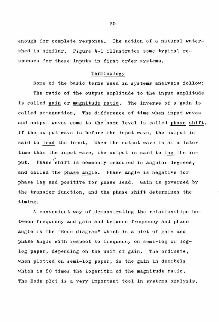
shed is similar. Figure 4-1 illustrates some typical re-
sponses for these inputs in first order systems.
Terminology
Some of the basic terms used in systems analysis follow:
The ratio of the output amplitude to the input amplitude
is called gain or magnitude ratio. The inverse of a gain is
called attenuation. The difference of time when input waves
and output waves come to the same level is called phase shift.
If the~t output wave is before the input wave, the output is
said to lead the input. When the output wave is at a later
time than the input wave, the output is said to ~ the inj,.
put. Phase'shift is commonly measured in angular degrees,
and called the phase angle. Phase angle is negative for
phase lag and positive for phase lead o Gain is governed by
the transfer funct'ion, and the phase shift determines the
timing.
A convenient way of demonstrating the relationships be-
tween frequency and gain and between frequency and phase
angle is the "Bode diagram" which is a plot of gain and
phase angle with respect to frequency on semi-log or log-
log paper, depending on the unit of gain. The ordinate,
when plotted on semi-log paper, is the gain in decibels
which is 20 times the logarithm of the magnitude ratio.
The Bode plot is a very important tool in systems analysis.
.A
1\
c o
21
IInput ---
Unit Forcing
..-___ -In pu t t---...;.. .• _/-i -- -
/'
t
Pulse Forcing
-- ",-Ou t pu t
~-" .............
t
Sinusoidal Function
Figure }i.-l.. Typj cal Helationship Het\\·ecll Input and Outpnt for Different Input Flll1ctj.ons fo}~ First Oruel' Syst81l1S.

22
For a first order system, the Bode diagram has two
straight portions. The two asymptotes meet at the "corner
frequency", which is the frequency corresponding to the
reciprocal of the time constant. The phase angle at the
corner frequency is 45°. The time constant is a parameter
that has the dimension of time. For a first order system,
the time constant is equal to the elapsed time when the
output has completed 63.2 per cent of its response. The
time constant is a parameter1which determines the speed of
the reaotion of a system when a disturbance is applied. A
typical first order system Bode diagram is shown in Figure
4-2. Two types of Bode diagrams for seoond order systems
will be int~oduced here. One is a combination of two first
order systems (a system with two time oonstants and two
corner frequencies or two first order systems in series.)
Another type is a true second order system, as shown in
Figure 4-3. The peak response for the seoond type of sys
tem occurs at the oritical response frequency, or natural
frequency, which is related to the time constant. The
height of the peak depends on the damping ooefficient of
the system. A plot of the template which shows the rela
tionship between natural frequency and the damping coeffi
cients is shown in Figure 4-4.
Dead time, transportation ~ or distanoe-velocity lag
or delay, is a waiting period between input change and the

(I I.>
o II frcqucn
o Q:; ---- ] () • J . __ .~_~~ __ +_.-_-__ <
0.2
g -20 ,,1
-loon 1 5 10 50 100
Freqncuoy· (Cycle per unit ttmc or radjans :;00
ver unit
..... ..... • ...j
rj :..:;
Fi db'
0
0.5--10 o.
o • -20 o.
0°
P -50
-150r--------.. ------------~-------~-~--.-------... --.--1i----.-
1 5 10 50 100
nin for ~n
order 1 ag
500
tjme)
Frequency (Cycle per Hlltt timp- or radtans per unit me)
Figure 1J·-3. Typieal Bode Dingram for Second 01'del' Sy~L(,1l1.

1'1 8.0
r I r---· I
2.0 ~
~::: ~--r-!
~O.251
0.10 t--I I
0.03 L - /-1.=. Damving
.;
= Natural
'; , .;-
...--rJ'j
C)
.1
.2 C> ~ c.c Co)
"d ---0)
,-..{
b.O ::::: -< -150 a.> 00 cj
..c: -180 ~ -200
O. ] 0.5 1.0 5.0 ]0.0 Frequency Ha tio ('\·/'\~n)
Figu re }i-!I.., Fre qu en cy He span sea r S e Call d-Ordc r Sys tems Sho,,-ing Damping Coefficients for Vari ons
Gain CUrY8S and PIHlse AngJ e Curycs"

25
beginning of output change. Dead time, Td , affects the
shape of the phase shift curve. An example phase shift
curve for dead time is shown in Figure 4-3.
The frequency response approach is an easily used
technique. If it can be used in hydrologic systems, then
prediction of runoff for a catchment may be easily calcu-
lated by digital computer when the transfer function of the
catchment is known. The transfer function may be found by
the inputs and the outputs ~f the past events.
Theoretical Analysis
The parameters which affect the response of a drainage
basin, or a natural hydro~gic system, include catchment F
shape, average slope, soil type, surface conditions, rainfall
intensity and duration, and land use. If we neglect the dy-
namic effect of the system and treat a drainage basin as a
reservoir with uncontrolled outflow, the outflow, or the
output (runoff), OR' is a function of the stage in the
reservoir and the hydraulics of the outlet system. (36, 39).
Therefore,
Similarly, the storage can be expressed as
m St = C2E 2
(4-12)
(4-13)
where e1 , C2 , ml , m2 , are constants, and E is a measure of

26
the reservoir surface elevation. In this study E is the
flow depth at the outlet.
Combining equations (4-12) and (4-13) gives
(4-14)
where C3
is constant, and n is defined as a nonlinear para
meter in this study.
Considering the dynamic effects, the storage is also -
a function of the rate of change of runoff. Therefore, II
equation (4-14) may be written as:
(4-15)
by the continuity equation,
(4-16)
where.6.I is the rate of inflow, ~ St is the rate of storage,
~O is the rate of outflow and6QL is the rate of total basin
losses (neglected in this study). Equation (4-16) may be
rewritten, by substituting rainfall excess and runoff in-
stead of the rate of inflow and the rate of outflow respec~
tively, as
(4-17)
Substituting equation (4-15) into equation (4-17) gives
dOR 6(C 4 ar- + C30Rn)/~t = R - OR (4-18)
Equation (4-18) may be written in differential form as

27
(4-19)
where A = C4 and B = C3
, both constant.
Equation (4-19) is the general form of the differential
equation for the hydrologic system, neglecting losses. It
is a nonlinear second order equation. When the system is in
steady state it means all variables are independent of time,
and then the equation_14-19) becomes
(4-20)
An nth-order system may be characterized by an nth~1-
order differential equation
dny;P' dn-ly dY a ---2 + a 1 1 + ••• + a ldt + aoY = X(t) (4-21) ndt n- dtn-
where Y is the output variable and X(t) is the input func-
tion. When n equals 2 the above equation becomes
(4-22)
If the system is linear, then
where Tc = time constant, ~ = damping coefficient and Gk
= gain constant which depends on the ratio of the output
and the input in steady state.

28
If the system is nonlinear, then
where f1(Y), f 2 (Y), and f3(Y) are nonlinear parts of the
function.
Comparing equations (4-19) with (4-22) gives
A = T 2 c '
and equation (4-19) becomes
(4-23)
Equation (4-23) has three unknown parameters, T , P , c :)---
and n. The time constant and the damping coefficient may
be obtained from a Bode plot, but the nonlinear parameter
n needs to be solved by trial and error. With this infor-
mation, the transfer function may be found.
The lag or dead time, is a function of the physical
parameters of a drainage basin which effect timing, such as
basin area, length in the longitudinal direction, slope of
the basin, surface condition, soil types and basin shape.
It also is affected by the rainfall pattern and intensity.
Since the basins used for this study were impervious and
also since a uniform distribution of rainfall was assumed,
surface condition, soil types and'rainfall pattern effects
may be neglected. Thus,

29
T d = f ( L , R , S, A a' 1{ ) (4-24)
where Td is dead time, L is the longitudinal length, S is
the average slope in the longitudinal direction, Aa is
basin projection area and ~ is basin shape factor.
Once the input and output data are obtained, the Bode
diagram may be plotted. From the Bode diagram, the time
constant and damping coefficient (if the system is second
order system) may be determined; then by using analog com-
puter simulation, the nonlinear parameter, n, may be found.
After the transfer function is found and with known dead
time of a catchment, the hydrograph may be easily calculated.

v. RESULTS
In this chapter the scope of this thesis will be out-
lined. Experimental results and methods of analysis will be
shown and briefly discussed.
Delay ~ Dead Time, Td
As mentioned before, delay time is a function of basin .
area, basin longitudinal length, basin shape, longitudinal
average slope and rain- intensity • •
Since the purpose of this thesis is to study the simi-
larity relationships and to try to apply systems analysis
to hydrologic system, the relationship between delay and
rain intensity is an interesting phenomenon.
" Experimental values of delay are listed in Table I.
Plotting delay vs rainfall intensity on log-log paper, a
straight line relationship is found. Figures 5-1 and 5-2
show this relationship. Plotting delay VB longitudinal
average slope, S, also shows a straight line relationship
on log-log paper. Figures 5-3 and 5-4 present this rela-
tionship.
Formulas which represent those relations were derived
by fitting a straight line through the data.* The formulas
so derived are:
*These straight lines were drawn through the data by eye.
30

31
TABLE I. DEAD TIME
Sl°Ee % 8 b 4 2
IR Delay
Basin sec. Td Td Td Td Td Td Td Td TrEe inLhr
I .83 44 43.5 53 51.5 60 61.5 87 86 43 50 63 85
34 40.5 '46.5 63 34 41 47 65
1.26 35 34.5 40 40.5 47 46.8 64 35
14 -, 15.5 18 25 6.26 14 -13.5 16 15.5 17 17.4 26.5 25.6
13 '15 17.5 26 13 15.5 17.0 25
~ 31 36 42 62 1.27 30 30 37 36.8 42 42.8 60 62
30 36 44 62 29 38 43 64
II I
J- 11.5 14 17 25 6.26 12.512 1 14 14.3 16 16.3 24 24.3 11.5 • 15 16 24
13 14 16 24
.83 36 42 49 48.5 64 64 37.536 •7 42.542 •3 48 64
27 30.5 36 47.5 1.26 28 27.5 31 31.5 38 36.5 47 47.5 III 28 32 35 47.5
27 31.5 36 48
11 12 13.5 18 6.26 10 11.511 9 ~~.513.5 19 18.9 10.510 • 6
11.5 • 19 11 12.5 14 19.5
'T'd= mean value

100 90
80 E I I I I~ S = 2% -=t
~,-tl' ..
.~'
70 I_ S = 11%
Go 1 S = 6%
L
-- 50 l-Q ' S = 'lJ ifJ.
""-" 110
0.;' :2
.-1
~
-:.;j 30 :'ij !,)
C \..·1 (-V
~ ~ ~ 20
10 • U ~ )
Hain Intensity (in/hI')
Figure 5-1. Helatiollship Between Dead rrillle and Hain Intensity for Basin rrype I.

100
90 80
70
(,0
50 s :::
S :::
'10 S ::: -. C,) C)
r./J
-- jO Q 2
'r-i r- ~~~ ~ I v-l c:... ~ \",-1
~
('j 90 0) ....
0
10 • /.1 .5 .6.7.8.9 1.0 2 3 lJ: 5 789
Rainfall Intensity (in/hI')
Figure 5-2. Relationship Between Dead TilDe and Rain Intensity for Basin Type III.

-.-..... .. 0 Cl,)
TJ'J '-""
Q)
:: 'r-! 8
"0 c: C!,)
~
100 90 80
70
60 ,{
50
40
30
20
10
9
R
. , 'Ii
1
34
---Basin r:I'ype I
--- Basin 'l'ype II
:: 1.26
2
::
in/hr
R ::
3 Slope
0.83
6,,26
If (%)
in/hr
~ 0
. II 111/ 11'
5 6 7 s
Figure 5-3. He 1a ti on shi p Be i;h"e en Bead rrilllC and Basin Slope for Basin TYVes I and II.
9

.-.,
0 CD t:J)
.............
C,)
-,..; 8
"d ttl G\)
~
100
90
80
70
60
~"50
110
30
20
10
9
R = 1.26
2
= 0.83 in/hr
= 6.26 in/hI'
3 .4 5 6 7 8 9 10 Slope (%)
Figure 5-- l1. Relationship Bet.ween Dead rrillle and BDsjn Slope for Bclsin Type III.

36
For basin type I.
Td = K S-·46R - .598 1 (5-1)
For basin type II
Td = K S-·46R - .598 2 (5-2)
For basin type III
Td = K S-·38R - .597 3 (5-3)
where Td is the dead ti·me in seconds, S is the longi tudinal
average slope, R is the rainfall intensity in in/hr, and KI ,
K2 , KQ are constants depending upon basin sbape, surface
condition, area and length. The values of KI , K2 , and K3
are 102.5, 93.5, and 76.3 respectively • . '1'. --.
From these formulas, it is clear that the dead time is
inversely proportional to the rain intensity raised to
0.598 power. This relation is independent of basin char-
acteristics. The relation between delay and slope does de-
pend on the basin shape. The exponent of the slope does
change with basin shape. The larger the slope and the rain
intensity, the shorter the dead time.
Response
Experimental data included three different input in
tensities, R = 0.83, 1.26, 6.26 in/hr, and four different
input durations, 5 min, 10 min, 15 min, and 20 min. Four
different longitudinal slopes for the basin were also

'. 37
studied, 2%, 4%, 6% and 8%. Input and output data are in
Appendix C except for the data for a duration of 20 min.
Some of the response data are plotted in Figures 5-5,
5-6, 5-7 and 5-8. Figure 5-5 shows the response for several
different slopes. Figure 5-6 shows the response with dura-
tion varying. Figure 5-7 shows the response for input in-
tensity varying. Figure 5-8 illustrates the effects of
changing basin types.
It can be noted that the response can be separated
into steady-state response ~nd transient response. The
transient response can be divided into a head part and a d
tail part, as shown in Figure 5-6. When t = 0, OR = 0 and
OR' = 0, then
Therefore
G(s) (5-4)
Equation (5-4) is the general form of the transfer
function for a hydrologic system.
A standard transfer function for a second order linear
system is
G(S) G~"e-STd
(5-5) =
T 2 2 2/,T s 1 S + + c c
where Gk is the gain constant.

.25 r-
..........
• 20 r-
j 0 I Q)
en I 0 .10 ! n
II
~
S
s = s~ T = 26 sec . d
0
Output
~
8
36 sec
8
38
s G% T = 29.5 sec d
.25 d (1
/ 0
H 0 1\ .20 I
J
I \
.10 ! \
\
~ _I-I I
0 2 q 6 8
s = 2% Td = 45.5 sec -I-25 1= .. - --------,
· J' CIte ~
I 0 C I'
! . 0 1\ .20~_, !\
.10
o 2 8
Time (min)
Figure 5-5. Response for Basin 11ypc III for n = 1.26 in/Ill' for Various Slopes.

.-(,) C,)
Ul
0 tl'"\
II .18
....:;. input g .16 ..- ~ "J! 0 y.. 0
ro a.> ~
~ d o
.-I -'r-! 'fl C'j
P
'" transient respon
I / , I rl curve ~
~ 'r-! '-'"
C> f/} ,.... • ,.... ~ ~ I'fJ
~
c:
•• -l.r-",
~
I steady-s t x response ,/, . .
'I. ;,( i, .,t"
-I...
10 Time
S = 8% I - ~ ,Type III OR - • 8.J in/hr
o 5 m x 10 111
Tn = TD =
T Interval =
output
.J
37 sec 38.5 30 sec
transient response curve tail
~
I ~
11 12 13 1 )1 15
Figure 5-6. Response for Different Durations (Basin Type III, S = , R = 083)
\.;~
\.0

o Il> UJ
1.25
O -I ·:>i
For R = For It
For R =
Inpu t,
40
6.26 ill/}ll"
1.26 in/hI'
0 .. 83 in/hI'
R = 6.26
I D D 6 6
o 1 00 ')-2~ -. Input, R = 1.26 ~ • ~~ r;---r~--------------------l i I 0 0 ---
/ 0 0
/ /
D
!.-Inpu t., R
"'--'"
-..... t{ -< .20 --~ I ~
<1 I X
DOD
.83
~ o c 0 (; '---'
o c
Il> r.F:i L_ ,-4 0.5 -0 0.. rJJ CD
.10 , r:r::
o o 1 2 3 4 5
Time (min)
rr d =
Td rr
d =
in!hr
6
11 sec
26 sec
37 sec
6 t = 30 sec
Input Duration = 5 min
7 8 9
Figure 5-7. Response for Basin Type III for Various Hatnfal1 Illtensities at S =

'" C) Das Type I Basin Type Basin Type II
r.tJ
0 11'"\ ~:~ II
~ 1.25 1.25~1----------~ ~5S7 <J ,.,......."
c:! ~ I .. 0 H ,rj "
1.0 .50 I .1iO I- .. ~
~ .r-l
"'--"
>~ ..;..)
.. 030 'M
'1'1 ~ C) • 5 ~ .20 .5 ,..... I'-<
H
~ ..., ,..J ...... .....-4
;::: H I
.10
0 o lb I l! l'b-o_~ I 0 0 2 li 6 8 a 2 '1 6 8 0 2 1:1: 6
Time (min)
Figure Response for Basin Type Varying~ R = 6.26 in/hr, S = 4%.
8
t!:'" ~

42
When n = 1, equations (5-4) and (5-5) should be equal,
therefore the gain constant KG for the hydrologic system is
unity.
In equation (4-23) when the dynamic effects of the
system are negligible, as in basin types I and II at slope
less than 2%J then the equation can be reduced to
daR = R (t - Td
) dt~·-~
f
and the transfer function becomes
G'( s) = e-sTd
(5-6)
(5-7)
Equation 5-7 represents a nonlinear, first order system
transfer fukction. Tc' is the time constant, about twice
the value of Tc •
In equations (5-4) and (5-7), if the system is linear,
i.e. n = 1, then the transfer function for the first and
second order linear hydrologic systems are:
e-sTd G(s) = T 2 2
c s + 2f' Tc + 1 (5-8)
The steady state response is constant and should theoret
cally be equal to the input for catchments without losses.
The difference in the results were caused by minor losses
and experimental errors in measurement, recorder reading
and calibration. Transient response curves were varied by
changing the slope of the basin, the shape of the basin and

43
the input intensity~ Transient response is, however, inde-
pendent of the duration of rainfall.
The results showed that changing the longitudinal slope
of the basin affected the tail part of the transient response
more than the head part. The larger the slope the faster the
response returned to the original level line. This effect
was not significant for basin type III and for basin types
I and II at slope greate-f than 2%. For basin types I and II
at slope less than or equal to 2% this effect is significant.
Roll wave phenomena were seen in the basin types I and
II at slopes greater than 4% at higher input intensities.
Roll waves ~re an interesting phenomenon in open channels • .MI. 'r
They appear as slight ,irregulari ties in the water surface,
ripples proceeding downstream, accelerating and increasing
in size until a breaking front is acquired. According to
Rouse (42) this phenomenon is due to the weight action af-
fecting the flow and is named "slug flow" or tlroll waves".
This really consists of a series of wave fronts of shock
type, and is formed at a constant frequency. In basin
type III, roll waves were not seen. The period of roll
waves seen in basin types I and II was short, and the ampli-
tude was small. The effects of the roll waves can be
neglected.
Since the responses reached steady-state, it is obvious
that the durations of the input were relatively long for the

44
pulse testing method. For the pulse testing method, the in-
put signal to the system is varied in a pulse-like manner.
The principal requirements in conducting a pulse test is
that the system dynamics are excited. But if the width of
the input is long the dynamics of the system are only moder-
ately excited. In this case, the gain curve was obscured or
non-existent at high frequency, especially for the square
pulse input. If a very short input duration was used, there
was no output, because-<a certain amount of water was needed
to wet the basin and also to provide, for some detention,
which{could not be avoided and would never become runoff.
In the experimental procedure, before every run, the
basin was dried. If the basin had not been dried, the out~I'"
put and the dead time for the following run was not correct
because there was some detention water in the basin, and
that reduced the dead time and increased the output.
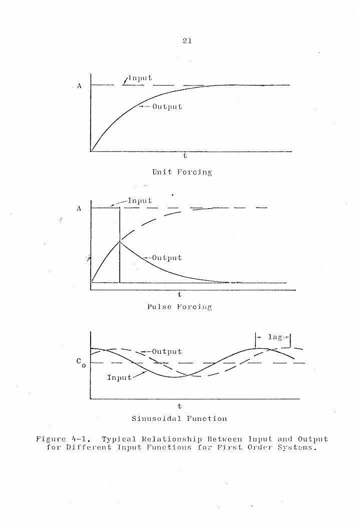
Bode Diagrams
Bode diagrams are plotted in Figures 5-9, 5-11, 5-12,
5-13, 5-14, 5-15 and 5-16. Magnitude ratios and phase
angles for selected frequencies were calculated by digital
computer. The computer program is based on the equations
derived by Hougen and Walsh (28) and Clements and Schnelle
(14).
[--I I-r -1 r I r -- - r I I-.···· r-~T-l fl--- ---r- I'· \ 11-r-, o ---------8:--------- -c=-===;:o::::=:::;:;-- j , , I 0 --- ., ~~ ~~~ I --------.~ -' --0-----0. "\ "\' I
I ----6-...... I I
-5 ~" .-~, ~\ ~-30o
-10 ~ .". Phrise" beO'in loopinO' ....... --.( I 1 I DUl'atlon = 5 mIll £'1 • be> 1 ,0 , 1 ! rOo
\,raln eg ooplng \ _-1-0
...-.. ~ ""C
......--
:::: ,,...I
ro o
o !:5 c-.w~---.::::n::__=.----.---~ 0 I
I ~ ~ ~
6-___ ~"" \~. I~ ~ ~ , . ,~, '.A "'0 ...-..
-:; [ 111 begIn 100pIllg --,--. '?1 -.)0 0..
D t ' 0' "'IJ
(0 ura lon = 1 mIn ~\ ~
phase begin looping --11 -600 ~ -10 I IT~' I ~
~ I
o 8 G==::;J~ I 0 ---t"r-- " ,,'
I - --(-: " d
-5 Duration = 15 min " [) _1-30 0
I Phase begin 1ooping--"1 I -10 ~ Gain begin looping ---4 ~-60o
U~JIIII I :) x 10-/ .1; 1 x 10":")
I . I~ lJ -2 ::> x 10
F'requcncy (cycles/min)
Figure Bode Diagram for Varying Durations, Basin rrypel, R 1'.26 in/hr S = 1.1:%
..:::Vl
.-'

20 ~~
15
\ I - ~ ~
>-4
'r-! S
'-"'" I
§ 10 'r-! I , ..j..J
C'j ~ ..... ,...J
c:::
5
\ \ ''-------
01 1 I) I 1 I 1_2 1 L_l~ -1 .;, 1-1 X 10 ) 1 x 10 1 x 10 4 x 1 0 .-
Frequency (cycles~nin)
Figure 5-10. Relationship Between Maximum Frequency of Gain Curve and Input Duration.
~ C\

o
-5
Type I
. -10
-... ,.0 "'::J
-..,.;'
~ .,....; ~ o
o
-5 Type III
-10 I UJ IIII 3 x lO~) 1 x
~
'rype II
I ~
I i i
-i I
-i I ,
~ -1
<~I ~
1_\~_J_J-.,Ll11J .. 1 ,_ I Q
1~ 3 x 10-~ 1 x 10⁻² 4 x 10--Frequency (cycles/min)
Figure 5-11. Gain Curves for Different Dasin Types at S = 8%, R = 6.26 in/hro
~ -.J

.-.... ~ '":j
----:::
'r-! C'j
C!i
5
o
-10
-20
a
-10
s = Ii = .83 Duration = 5 min
s = 6%
H = 6 0 26 in/hr
Duration = 5 m
-20 I I I I I I ---L 3 x 10⁻³ 1 x 10⁻²
Figure 5-12. Bode-Diagram 'for
\ 0
t~ ! I ~I 0°
I I -j
!
r-!-1200
J ~l..\ Duration = 5
..:::--r.tJ
o
~li.-,--I 1:-.....1-
1 1----, 4 x 10-) 1 x 10⁻²
I_GOO '--If: -x-,. -l-'-O----'7"itl
I --'1
~ __ ~~ ________________________ ~1_1200 5 x 10⁻²
equency (cycles/min)
put Intenstty Varying at S G%, Basin Type III.
10 FTl-T-rrrT-·····T----r-·-l-T1lllll-?~-r .. -- 1 pi. ----l Goo
I
~
o t-----e--1
l : "
\ I \ , \ I t1
'. I I \
_____ ~~I 0
-60 0 :; -10 o Gain
-----:::
.,-l 6, Phase c:
C!:i Duration = 1 min
-20
\ \ \ ~-180o
~,~ L-L-' __ "-_. lJ~LLlL ___ I ~ ~ 1 x 10~2 1 x 10⁻¹
-120 0
Ii: x 10-1 3 x 10 ..... 3 Frequency (cycles/min)
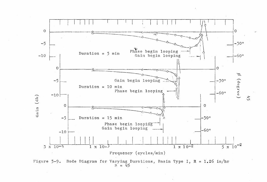
Figure 5-13b Bode-Diagram for S = 8%, R = 1026 in/hr, Basin Type III.
..::\C

i-TTl II If 11- -l--T--Il-rn---···· 51-
it:'
...-
o 1---0-- ~O:.-=-=---:-~=-..;:.~-o-==---~_-=-~ --~~ -----.Q.....---..---o. ..
~-~ ~,
"
.----o------~
,=1 -10 ~ '6--...-
:::: ...... ~ v
-20
3 x 10⁻³
o
6
Gain Phase
Duration = 1 min
_0 1 1 x 10 ~ 1 x 10-Frequency (cycles/min)
~
r j-l :00
! i
_-----I)--__ ~i a I
I . i -
-1-60°
I ~
." ---,l20 Q
80°
ll.X 10-1
Figure 5-14. Dode-Diagraul for S = G%, R = 1 0 26, Dasin Type III.
V1 o

5
o
_, -10 ,::; '":j --c: ,,... ("j " ... -'
-20
f5
30° ~~
o
~---6-'----'6-
'"'----~---. .o ~,~
"",
"
~~ I
__ J-GOo
I o Gain
/:,. Phase
min Duration = 1
_-,-120°
~ 1 ~ 3 x 10-) 1 X 10⁻² 1 x 10- 4 X 10-J
Frequency (cycles/min)
Figure 5-15. Bode-Diagram for S = 4%, R = 1.26 in/hr, Basin Type III.
\ .. n r-t

fTTn- J1 ) [ I I I I I lir-l-I I
.. ""'", 30 0
o
~ .
-0 --. '.-.-
-6------.6.... - -.--~
-10 L "~ I 0 Gain ~ L f:l Phas e "-
-. ...:::l
o
~
-,-60 0
I
...... I . ..., ~
~ -:20
Duration = 1 min
-120°
-30
t I IIII ~ 3 x 10⁻³ 1 x 10⁻²
•• ~().-O
-180°
L I I IJl1 XI I._~.J ~ -1
1 x 10⁻¹ . Frequency (oycles/min)
4 x 10
l:jligure 5-16. Bode-Diagram for S == 2%, R = 1.26 ill/hr, Basin Type III.
\ .. ;1 (\J

53
The equations were derived by converting pulse to fre-
quency response form utilizing the theory of Fourier trans-
formation. The magnitude ratio or gain is the ratio of the
output frequency content to that of the input. Thus
(T . t = )0 yy(t)e-J dt (T . t
)0 Y x ( t ) e - J d t
M.R.
where M.R. = magnitude ratio
Ty ' Tx = width of-system output pulse and input pulse
respectively
¥(t) = arbitrary function of time of system output
x(t) = arbitrary function of time of system input
j = ;-:::;-~1'~
Q= selected frequency
t = time
The integrals involved in the above equation can be
evaluated approximately by changing the equation to summa
tion form. When the time intervals for both input (inde
pendent) and output (dependent) variables are equal, the
-gain and the phase angle can be evaluated by the following
equations.
and
M.R.(CU) =JRe2 (U) + Im2(GJ)
¢ = tan-l(Im(~)/Re(~»
Re(W)

54
Where ¢ = phase angle n
(ID6.t) Cos (wkbt) A =.6t 2:y YK=I
n (k.6t) Sin(wk.6t) B = 6ty2: y
K=I n (Wt) Cos (willt) C =.6t 2:x x K;,
D n
(iAt) Sin (u.li.6t) =~txLx K::,
Re = real part of system performance function
1m = imaginary part of system performance function
x(:iAt)= the value of. --the independent variable
y(~t)= the value of the dependent variable at time k6t
k = the interval number 4 The performance function is defined as "the ratio of
the Fourier transform of the output pulse to that of the
input.t! (2~) Figure 5-9 shows the Bode diagrams for different ~nput
durations. It illustrates that varying the duration shifts
the gain curve. Since the Bode diagram shows the dynamic
effect and the time effect of the system, the longer the
duration the more suppressed the dynamic effect, and the
less significant the Bode diagram.
The gain curves and the phase shift curves are folded
and looped at higher frequencies. For example, in Figure
5-9, the gain curves begin to loop after UJ is equal to 0.02
and the phase shift curves begin to loop after ~ is equal
to 0.015 cycles/min for the duration equal to 5 min. This

55
is because at the higher frequencies the input pulse does
not contain enough harmonic content to produce accurate re-
suIts. The harmonic content of a pulse is related to the
shape and width of the input, and the frequency at which the
the magnitude ratio is computed, and also related to the
time interval used for output measurement. For a given
shape of input pulse, the frequency at which the gain curve
begins to fold depends mostly on input duration. The
shorter the input duration the higher the frequency. This
is shown in Figure 5-10. The phase shift curve is looped
earli~r than the gain curve.
Figure 5-11 shows the gain curves for different basin
types. It indicates that the gain curves for basin types I f·
and II are almost the same, which means the effect of chang-
ing the size of the basin proportionately can be neglected.
Figure 5-12 shows the Bode diagrams with intensity
varying. It is noticed that for large input intensity, the
dynamics effects of the system are shown more clearly by
the gain curve, but the phase shift curve is folded earlier.
This is because the higher the input intensity the more the
system dynamics are excited.
Figures 5-13, 5-14, 5-15 and 5-16 show the effect on
the Bode diagram of slope variation. The change of gain
curves and the phase shift curve due to the changing of the
basinlongitudina1 slope is not large for slopes 4%, 6% and
56
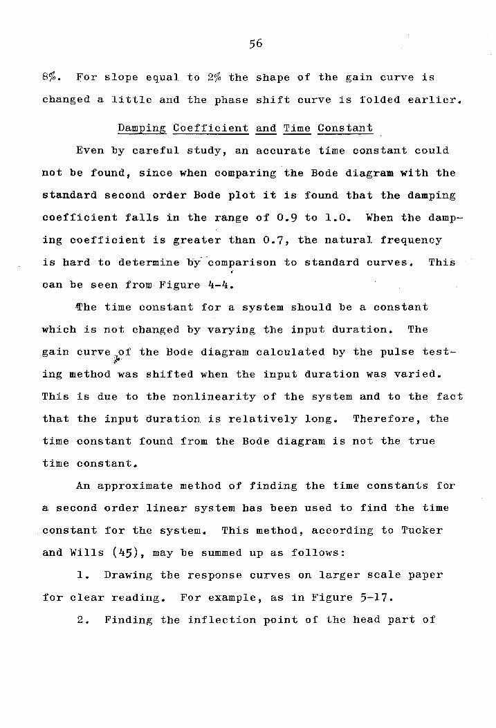
8%. For slope equal to 2% the shape of the gain curve is
changed a little and the phase shift curve is folded earlier.
Damping Coefficient and Time Constant
Even by careful study, an accurate time constant could
not be found, since when comparing the Bode diagram with the
standard second order Bode plot it is found that the damping
coefficient falls in the range of 0.9 to 1.0. When the damp-
ing coefficient is greater than 0.7, the natural frequency
is hard to determine by comparison to standard curves. This t
can be seen from Figure 4-4.
~he time constant for a system should be a constant
which is not changed by varying the input duration. The
gain curve "of the Bode diagram calculated by the pulse test""
ing method was shifted when the input duration was varied.
This is due to the nonlinearity of the system and to the fact
that the input duration is relatively long. Therefore, the
time constant found from the Bode diagram is not the true
time constant.
An approximate method of finding the time constants for
a second order linear system has been used to find the time
constant for the system. This method, according to Tucker
and Wills (45), may be summed up as follows:
1. Drawing the response curves on larger scale paper
for clear reading. For example, as in Figure 5-17.
2. Finding the inflection point of the head part of

Final yn]uc 11.118
Origtnal level
T a
57
'l'imc ill millutes
Figure 5-17. --T)rpical Process Heaction Curve (Dead Time Neglected)o
1.O~
1\ .9--
. s
oJ ~
~~ .. 2
.1
o o .1 .3 .4 .5 .6 .7 .8.9 1.0
Ftgurc 5-18.. Graph for Finding: Equivalent Time C011 S tan t fro m Pro C (! S sHe act ion C u rv e Q
(A f t e r Tu eke r a 11 d \\' iII s ( It::3 ) ) •

58
the 'transient response curve. The inflection point is de-
fined as the point where the slope first starts to decrease.
Drawing a tangent line through the inflection point.
3. Measure Ta and Tf and find the ratio Tf/Ta.
4. On the curve reproduced in Figure 5-18 mark this
ratio on both coordinates as shown at points 1 and 2. Con-
nect the two points. If the ratio is larger than 0.73,
there will be two intersection points. Either one of 'the
two intersection pOint~-~li~e point M or S) will give a
reading on the two scales. The two time constants are given
by multiplying these two values by T • a
5. If the ratio TflTa is equal to or less than 0.73,
there will~e only one intersection point or no ~ntersection
point. If the ratio is equal to 0.73, then a time constant
equal to 0.365 times Ta is the only time constant. But when
the ratio of TflTa is less than 0.73 the time constant found
by this method is less accurate, the smaller the ratio the
less accurate the time constant. To use this method, it is
better to use a small time interval for the output, since it
gives a better and more accurate response curve.
The time constants found by this method were not satis-
factor~ either, since they were too small. This is because
the system is not a linear system. Also, because the re-
sponse reaches to its steady state value very fast, the
ratio of Tf/Ta is much smaller than 0.73.

59
The time constants were found finally'by trial and error,
since with the information given by the Bode diagram and by
the approximate method, the neighborhood of the time constant
is not hard to find. Figure 5-19 shows the effect on outflow
of varying the time constant in a second order system. The
time constants were between 0.45 min and 0.60 min for basin
Type III. For basin types I and. II, at slopes greater than
2%, the time constants were between 0.48 min and 0.65 min.
For slopes equal to or.·less than 2%, the system may be ap-f
proximately simulated by a first order linear system with a
time ponstant of about 0.8 min. ~
The time constant is a function of input intensity,
basin shape and basin slope, the larger the slope the sm~ller ~~
the time cg~stant and the larger the input intensity the
shorter the time constant. For a natural basin, it should
be a function of the basin characteristics and input intensity.
Nonlinear Parameter, n
There is no simple 'way to find the nonlinear parameter,
n. A trial and error method is suggested. The value of n
obviously depends on basin shape, slope, and the outlet size
and shape. According to Prasad, "For a basin with vertical
wall around and with a proportional-weir type outlet, the
nonlinear parameter n is equal to one." (39). Figure 5-20
shows the effect of varying non the outflow for a second

0.6
0.5
0. /1,_
0.3
0.1
a o 1
Ftgure 5-19.
= 0.5
-- T = 0.65 c
T = 0.80 c
T = 1.0 c
~
.. ir ..
1.0 rm Input '" /~
if;~
L" t, 'J I . ,J J_
a 5 10
\
n = I'~
f = 1.
rr = 3.0 c -
fJ.'ime (min)
2 3 '1 :> 6 7 8 9 Time (min)
Effect of Varying Time COllstant T on Outflow for 1\ Second Order Sys tom (n = 1 ~ f) = 1).
C\ o

.p ~ P-c
.p ~
0
/"" Input /' 1.0 --- --l
I
0.,8
o .. ~()
0.4
0.2
o o 1 2
61
= 10
n = 5
= 2.5
Input Intensity = 1
Damping Coefficient = 1
Input Duration = 1
= 1.5
11 = 1.0
3
Figure 5-20. Effect of Varying n on Outflo,,- for A Second Order xronlinear System.

62
order system. For slopes greater than 2%, the nonlinear para-
meter for basin types I and II was found to be about 1.15.
For basin type III, it was about 1.25. When the slope was
equal to 2%, for the plane basins (basin types I and II), the
system becomes approximately a first~order linear system.
This is because when the slope was small there was some water
gathered at the end of the basin which could turn the outlet
of the basin to a proportional-weir type decreasing the non-
linear parameter n to unity. This phenomenon also could hap-
pen at higher input intensity. The detention water in the
basin would also reduce the dynamic effect of system and make
it negligible, especially for small input intensity. The
dynamic effect for a system depends upon the input intensity ~;;"
and the depth of the detention water in the basin, the larger
the input intensity the more significant the dynamic effect,
but the larger the depth of the detention water, the smaller
the dynamic effect .•
Transfer Function
The general differential equation describing 'the system
is
T 2 d 20R n-l d OR + 2(J Tc n OR =
c dt 2 dt (4-23)
The Laplace transform of the above equation is

+' 2PTc n [OR(S)] n-l [SOR(S) - 0R(O), + Qn(S)]
= R(s)e-sTd
when t = 0, OR = ° and OR' = 0, then
Tc 2
[s20R (s)] + 2,P Tc n s [OR(S)] n + 0R(s)
= R{s)e-STd
Therefore
G(s) e-STd
(5-4)
Equation (5-4) is the general form of the transfer func-
tion for a hydrologic system.
A standard transfer function for a second order linear
system is
G(s) , G' -sTd /p. . ~ e
= --~~------------Tc
2 s2 + 2f Tc s+l
(5-5)
where Gk is the gain constant.
When n = 1, equations (5-4) and (5-5) should be equal,
therefore the gain constant Gk, for the hydro19gic system is
unity.
When the dynamic effects of the system are negligible,
as in basin types I and II at slope less than 2%, then the
equation (4-23) can be reduced to
2f'T c n-l dOR ( ) nOR = R t - Td
dt (5-6)

64
and the transfer function becomes
G(s) (5-7)
which is a nonlinear, first order transfer function, where
Tc t is the time constant, about twice the value of Tc •
In equations (5-4) and (5-7), if the system is linear,
i.e. n = 1, then the transfer function for the first and
second order linear hydrologic systems are:
and
G(s)
-sT G ( s) ::i.i.i. e d
T f S + 1 c
respectively.
(5-8)
(5-9)
Equations (5-4), (5-7), (5-8) and (5-9) all are the
transfer functions for hydrologic systems. But, equations
(5-7), (5-8) and (5-9) are three special cases of equation
(5-4). Therefore, equation (5-4) is the general transfer
function.
Hydrologic systems are different, one from the other,
but most of them are one of these four types--first order
linear or nonlinear, second order linear or nonlinear.
Since the general nonlinear expression is all inclusive,

65
the transfer function of hydrologic systems can be writt'en
in the form of equation (5-4)0
It was found that for basin type III and for basin
types I and II at slope greater than 2%, the transfer func
tion of the system was in the form of equation (5-4). For
basin types I and II at slopes equal to or less than 2%
the transfer function was in the form of equation (5-9), i.e.
the system could be described by a first order, linear
equation.
Digital-Analog Simulation
Often the equations required to adequately describe a
complex system oannot be solved by any rigorous process.
This situajion has led to the extensive development and use
of machine aids to computation, such as analog and digital
computers whioh now play an important role in engineering
analysis.
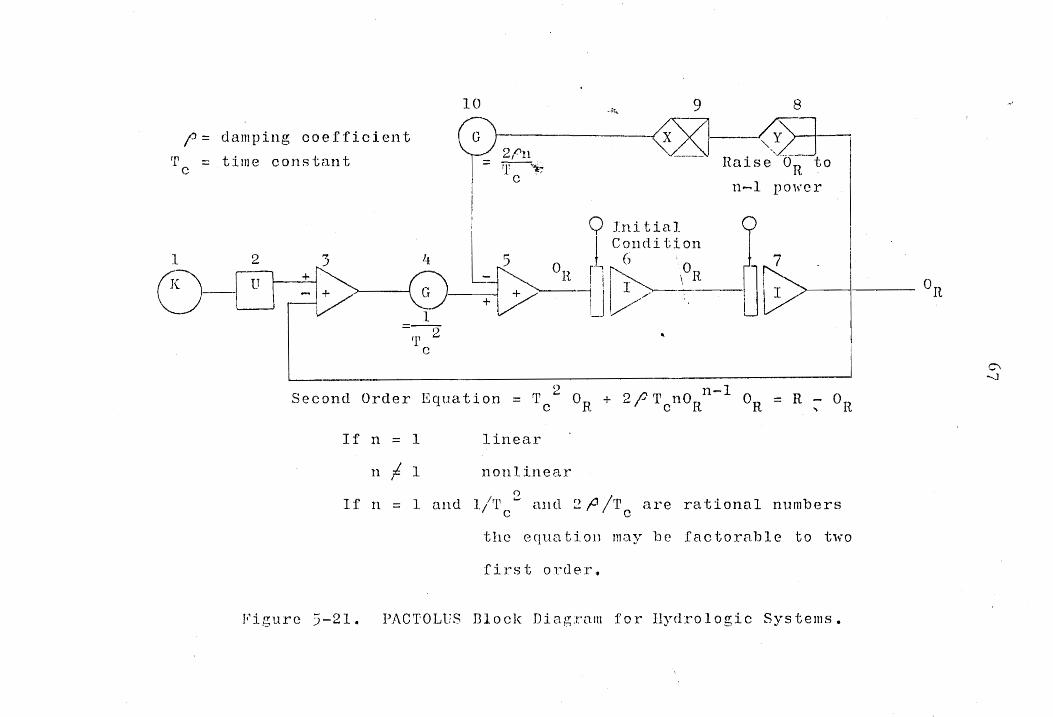
A Digital-Analog simulator program, oalled PACTOLUS (7),
uses operational blocks to synthesize a problem as an
analog-oriented program on a digital computer. The tech-
nique of drawing a PACTOLUS Hock diagram for a differential
equation is that of drawing a block diagram for an analog
computer. One first has to solve the equation for the
highest derivative term. Then, according to the new equa-
tion, one draws the block diagram. Each block must have a
number and a symbol to represent the operation of the block o

66
A primary difference between a PACTOLUS block diagram and
an analog computer block diagram is that in a PACTOLUS
block diagram the integration block only integrates the in-
put function; it does not change the sign as in an analog
computer block diagram. The sign in PACTOLUS is assigned
in a summation block.
Equation (4-23) may be solved for the highest deriva-
tive term as
d 20 R - 0 2 f 0 n-l d OR R R - n R (5-10)
dt 2 = T 2 Tc dt c
r
(5-10) The PACTOLUS block diagram for equation is shown in
Figure 5-21.
Figure~ 5-22, 5-23 and 5-24 compare the output calcu-I'
lated by analog-digital simulator and the experimental re-
suIts. From these figures, it is clear that for a definite
system (definite basin shape, outlet, and slope) and a given
input intensity the time constant is a constant, i.e. the
time constant is independent of input duration.
Application to Natural Basins
A number of sets of data for natural basins in Detroit
metropolitan area, Michigan, have been tested by the tech-
nique of systems analysis o Part of the data were used to
find the basins' parameters (such as time constant, non-
linear parameter), and part of the data were used for
10 9 8 .. ir""
(J damping ooefficient 1--0J! rr == time cons tan t c
2pn ry-~ Huise OR to
1
C) 2 :3 '-1
rr C
I I
o n-1 power
li Q Ini tial
~-~ r~II~\~ .. : 0- 7
I 1+/ -1J 1/ +v I V "
Second Order Equation = Tc2
OR + 2(JTc noRn - 1 OR = R ::-- OR
If n = 1 linear
n -I 1 nonlinear
If n f)
= 1 Gnd l/rr ~ and 2 (J jrr o C
ers are rational nn
the equa tioD may be factorable to t1","O
firs t -order ~
Figure 5-21. PACrrOLUS Dlock Diagram for Hydro logic Systems.
On
C\ .......j

---... d
<
~
~ p.. ~
H
"V ~ ro
.;..:> ..... -' ~
.;..:> ~
0
68
Basin 'Type- 1
S = 8%
H = 1.26 in/hr l )( 10 mill dUl'atjoll
o 5 min duration o '7 -
"J [ /"" ]np17t lcye]
, , )'0. " /. ~ ,r, J..; '. ' X x; ,.. \ - - L-c~----'---r-:--;r~-,( ~ " v------y:-~ .. \~ >'~\ c\ j 'I- \
0.2 / LAotnal data ~
\
11'-- Digi tal-analog \. slmulation curve '\
0,,1
o o
0 .. 3
0.2
0.1
o ,0
I \~lc = 0.52 .,\ - I " n = 1. 15
JI' x r f= 1.0 \
JL r c~ I L I x~ 5
X 10 mill duration
o 5 min duration
level
o :-:... 0\ 'j.., x'n'~(J ot,,\
1'. ;>( '\
Actual da tu \ o.
5
10
Basin Type III
S = 8%
R = 1 .. 26 in/lll~
~ ){ 'f.'f...". f '/.}.( \
Digital-anCilo,?'\ simulation CUl'y~
T = 0.50 c n = 1.25
/'= 1.0
Time (min) 10
Fig u r e 5 --~ :2 () Com par i S 011 0 f n i g ita 1 -: \ II a 1 (Y!E S i III i! 1 a t ion CurYe alld :-\0 tual Data for DIll'tl tioll Varying.

1 .. II
1.0
0.5
----ro <: ~
0
+.::l
<l ~< ~
~ ""-"
+.::l ::> ~ ,..... ,.....
H
H 0.15 0
~
~ ~
+.::l ;j 0 .. 10
0
o
0
Input lcyel
o 0 c 0 C C
"-- !\--Actual data c
5
L-
rlnPllt level
'- - ---
Rustn Type I
S = 4%.
H = G.~6 in/hI'
r-Digi tnl-Allalog Simulation / Curve
n = 1.10 'Ii = 0 .. 52 c
f= 1.0
10
R = 0.83 i.n/hr
L 1 c~ L Actual data~ /----Dj.gj tal-Allalog \1 Curye
Simulation
\
n=1 .. 15
rp = .. G2 c
0\ := 1.0
I _ Q 5 10
T i rn e (nd 11 )
Figure 5-23.. Comparison of Dlgital-.:\nnlog Simulation Curye and Actual Data for Input Intensit.y Varying.

c:::: -..j..;)
::s ~ .-I ;...;
H
f..; 0
-;..: !""'( .-p...
...J...:> ;j 0
70
Bas in 'Iype I
S = 2~~ H = G. 2 (; in / h l'
First order digital-nualog simulation curve
'}1 = 0.85 c
f' = 1.0
17 = 1.0
o ) I I .. .l...-.l;Oi--...I..--_-'-_-.l......_--L_-.-:L ___ • _.i--_-".-_-'-_"""': - ___ _
o
~
o.3Y Input
0 o.zt- -leyel
0.1
o o
5 rrime (min)
Bas in ]1ype I
S = 2%
10
R = 1.26 in/hI'
First order digital-ann]og simulation CUl"'e
T = 0.90 c
f> = ].0
n = 1.0
rrime (mill)
Figure 5 2'1. Comparison of Digi tal-L\nalog Simulation and Aetual Data by First Order, Linear System for Basill Type I, S = 2%.

71
checking. The values of the parameters were found from Bode
diagrams which were calculated by applying the pulse testing
technique to the data. The method of selecting the base line
for separating surface runoff and infiltration from precipi-
tat ion was to take a horizontal line to cut the precipitation
rate graph at a level such that the total volume of precipi~
tation above this line equaled the total volume of surface
runoff. The computer program for these routine calculations
are in Appendix A. After the parameters of the basins were
found, the outflows were compared with the actual data.
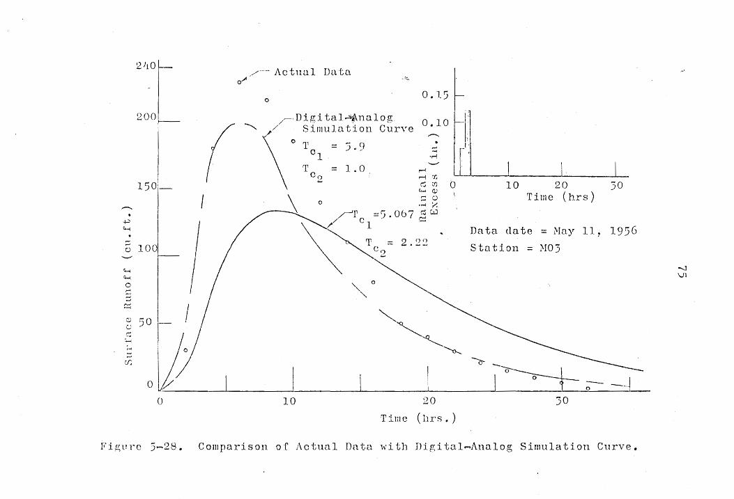
Figure 5-25 shows the Bode diagram calculated from the ~
data taken at station 3 at Macomb County, April 7, 1959.
Curve A is the actual gain curve which was separated into
curves B a~ C, both standard, first order, linear system
gain curves. Therefore the system can be represented by a
second order linear system which is a combination of two
first Drder linear systems. The two time constants found
from curves Band C were 5.067 and 2.22 respectively. By
using these time constants in the PACTOLUS program, the
outflows for the rainfall excess at April 7, 1959, April 5,
1957 and May 11, 1956 were calculated, and are plotted with
the actual surface runoff data on Figures 5-26, 5-27 and 5-
28, respectively. Results for April 7, 1959 and April 5,
1957 show satisfactory agreement, but for May 11, 1956 the
simulation is poor. A little correction of the time

db
a
-10 1---
c ..... 20 'r-< ..... '1.1 c;
-30
Data Date=April 7, 1959 Station=M03
6
A
B
C
Phase Shift Curve
Actual Gain Curve
Standard First Order. with T = 5.067 h~ c 1
standard First Order, with T = 2.22 hr c 0
~
f1
C\ _30 0
"'V,/" ,--13 _60 0
"", 6 . "~
-----.&,-----n ~ , -", ~
-~ ", .,,-_.,/' ""-, A
-90 0
20°
Linear Gain Curve, ~ .. 1)OO
I -+180 0
I
I Linear Gain Curve,
-I I I I
I
--->---L---.-J--.L-I1LJI1l__ I I I I I I -I 0,,01 0 0 1 100 2"Q
Frequency (radians/2 hr)
Figure 5-25~ Dade Diagram for Natu~al Busin, Macomb County, Michiganp
....... 1 Iv

160
-.. lIla •
4.:J ~
• ;:: 120 0
'--"'
c...... ~ 100 :.':) ...... .....
c::: 80 C)
:> ~
c.....; Go ;....; .-~
110 (--I
20
0
0
Datu date = April 7, 1959 station = NO)
-..
::: '''';
----t/)O~15 r.n (l)
o xO.lO :il
~ ---:
"" i.r-""
cj (';..,.;
~ .~
I It o LLL_ r- Digital-Analog C"j
lSi III U 1 at ion C u rv e c:::
" "'-- Ae tunl
Data
10 20 30 Time (hI'S)
'10 50
Fi.gure 5~26. Comparison of the Actual Data with Digital ..... Analog Simulation Curve.
.....,j
'vl

180- .. --
---I-=> "--l
160
l'lO
..: 120 o
"'-""
'H 100 c......
o ;::::: -,...; ~
(J) C) ,'.i
~ ~
Cf]
80
60
'10
20 I 10
o
o (:)
--•• 11"" ,.c: C)
~ .2 ,,-I
"'-""
~ rtl r.n C,) <:.)
>< w .1 r-I
/ __ Actual Da ta ~ .
:-1 r::I
t...,.
.-; ....
'1""'1
o c-j
et: a
0 20 . 110
Digital-Analog Simulation Curve
Time (Hr.)
T = 5.067 c 1 Data Date = April 5, ~ 2.22 Station = MO}
1957
0
'--c, , L :r-o--~ 0 10 20 30 '10 50
rrimo (Ilr .. )
Figure 5 .... 27. Comparison oj:' Aetna,I Data 'wl tIl Digi tal-Analog Simulation Curye.
-.l
2'10
200
15°1-
- I -j...)
~-1
o 100 --~ ~
0 ~ ,.....
c:::: I ? 50 '-' ~
::.... , .... ...., ~
o
//--- Ac tua 1 IJn o~
o 0.1.:;
;1 r-- Dig ita 1 ~~ n a log 0 • 10
-...... \~/' S imulu t ion Curve --: o l' =:.> .. 9 :::
01
.:::;. , I· T = 1.0 ...... , W -0
C """;JJ , 0 () a ) 2 c:;:n 0 1 ,;;.. ~ ~ Time (hrs)
\ 0 .,... ~ _\ rr =5. 06 7,5w
10
~cz= 2.Z~ ~o
20
Time (hI'S.)
Data date = May 11, 1956 station = M03
30
FigPT'C 5--28. Comparison of Actuul Data \\"i th Digi tal-Analog Simulation Curve.
--.l VI

76
constant shows better fittingo For finding the reasons, the
original data have been carefully studied. Figure 5-29 shows
these data. It can be concluded that the surface runoff data
for May 11, 1956 was not caused by the rainfall data of May
11, 1956 alone, since the dead time for the data was too
short compared with the other two sets of data. The follow-
ing table shows these comparisons.
Data Date Total Rainfall Volume! Dead Time --Basin Area (in.) (Hrs.)
May 11, 1956 0.27 2
Ap~il 5, 1957 0.51 13
April 7, 1959 0.67 12
The dead time for natural basins was usually long,
especially for small rainfall intensity. The rainfall
volume for May 11, 1956 was smaller than the rainfall volume
either of April 7, 1959 or April 5, 1957, but the dead time
was much shorter which is contradictory to the notion that
the larger the input intensity the shorter the dead time o

en o
0.2 1T Haillfall
I .1,1
o 1 1,-4-
· L o
10 20
0.2
0.2t
0
0 10
30
77
Hainfall begjns April 7, 1959
Infiltration =1111.62 100 en. ft.
n n!i I
40 50 60 70 Time (hI's) .
-;..:l
1200 ~ Rainfall begins 1
April 5, 1957 o
Infiltration = h~5 100 ~
°IH'lt.] _ i 30
Time (hrs)
Rainfall begins ~lay 11, 1956
Infiltration = 328.86 ell. ft '.
60 rJ)
250
200
]00
20 SO 40 50 60 Time (hI's)
Figure 5-29. Hainfall and Surface BUllOff Data ..

VI. DISCUSSION
Hydrologic systems are very complex. Every catchment
is different from others; therefore there is no accurate
method or equation which is applicable to all kinds of catch
ments for prediction of storm runoff o Systems analysis tech-
niques are useful methods for finding the transfer functions
of a system, which then provides a mathematical model of the
system. Application of systems analysis techniques to hy-
drology has been tested and the results show that it is use
ful, not only for artificial basins, but also natural catch-
ments. Any catchment with some previous data is susceptible ~
to the use of systems analysis techniques to find the trans-
fer function for rainfall excess and runoff, and that func-'f'· .' tion can tben be used for future prediction of runoff.
The general differential equation (Eq. 4-23) for hy-
drologic systems, derived by treating the drainage basin as
a reservoir with uncontrolled outflow and by adding a dynam-
ic effect term, is a useful form which not only represents
second order linear or nonlinear hydrologic systems but also
represents first order linear or nonlinear systems. The
order and the linearity of hydrologic systems can be deter-
mined from the Bode diagram which is computed by applying
systems analysis techniques to the previous data of that
catchment.
78

79
The dead time, which is the important part of the time
to peak, is a function of basin physical characteristics
(such as area, length, shape, slope, surface condition, etc.)
and rainfall intensity. The writer believes that the func-
tional form of the time to peak should be the same as dead
time, not only a function of basin characteristics as Wu
(47) derived, but also a function of rainfall intensity.
Wu's equation
is dimensionally incorrect. If the rainfall intensity is J
included, the dimensions may become correct. The suggested
functional form for time to peak is
:p. tp = K A! LY SZ RW
where tp is time to peak, K is a dimensionless constant, Aa
is the basin area, L is the length of the basin, S is basin
slope, R is rainfall intensity and x, y, z, ware exponential
constants. Further study is necessary for determining the
exponents and the constant K.
The time interval of observation used in this study is
somewhat large, and the duration of the input pulse is rela-
tively long. A shorter duration and a smaller time interval
are recommended for further study. A larger input intensity
will also give better results for the same duration. The
sine wave or smooth curve pulse input instead of square pulse

80
input is suggested, requiring an automatic control for
generating the input. A sine wave input would permit fre-
quency response testing, adding to the validity of results
deduced from the Bode plots found by pulse testing.
The time constant for natural basins depends on the
basin's physical characteristics which also should include
the soil moisture deficiency of the basin.
The similarity criteria for time derived by Grace and
Eagleson (22) does not quite hold for the timing terms used
in system analysis. This is shown in Figure 6-1. The lines
A and At were calculated according to the dead time data for
basin type I by Grace and Eagleson's equation,
.2. when e p = em' tr = (Lr)2. Lines Band B' were plotted ac-
cording to the data measured for basin type II. The dif
ference is 10% and 12% for rainfall intensity 1.26 in/hr
and 6.26 in/hr respectively.
The dynamic reactions of basin types I and II (the
plane basins), with the slope equal or less than 2%, are
different from the other slopes which can be simulated ap-
proximately by a first order linear system. This is coin-
cident with what Grace and Eagleson (22) stated. The reason
is that when the slope was small, the detention water
gathered at the end of the basin, which turned the basin

81
200 --- ---.--.-."-------,.~
E~pe~:iJ:~~~7~1 f~r ~C~~~
100
80
Type II --
According to Grace and Eagleson1~S Similarity Relation
r tan 8 1 i-t = L p.1 - -r r'-\ tan f} I _
mJ ==1 --i --!
i ---'I --, j
o 150 R = 1.2() tU/hr
~ -.J
~ --l .8
40r--o . ,. ~ "'B~ ! ~ .
o r- ,~>tI
301
L I
20r n = 6 .. 2G in/hr
10,
9L'..l..--i ~_~I llLiltl~ll1dB 1 2 3 4 5 G 7 8 9 10
S 1 0 po (~~)
Figure 6-1. Comparison of Actual Data and the Calcll-1 a t ion by Grit c (' and E a g 1 c S 011 1 S Sind. 1 a r j t Y' HelnLioll for Dead Time ..

82
into a reservoir with proportional weir type outlet; there
fore the nonlinear parameter was reduced to unity. This
also reduced the dynamic effect of the system and made it
negligible.
The problem in applying systems analysis techniques is
that when the system linearity and order is not known there
is no standard method for determining the form of the trans
fer function or the parameters.

VII. CONCLUSIONS
After a careful study and analysis of the experimental
data of the hydrologic systems, using different input inten-
sities, different basin areas, shapes and slopes, the follow-
ing conclusions may be drawn.
1. Systems analysis methods are applicable to hy-
drologic systems, not only to artificial ones but also to
natural hydrologic systems. Some analyzing technique is
needed to find the time constant for a nonlinear system
from ~asin parameters and rainfall intensity.
2. The relation between the dead time and the input
intensities for artificial hydrologic systems can be repre'P~
sented by the equation
where Td is dead time (lag) and R is input intensity; f
represents a function dependent upon basin characteristics.
Further study is necessary to find the relation between
dead time and basin characteristics o
3. The damping coefficient for hydrologic systems is
close to unity, especially for natural basins. This means
that the basin is critically damped if the second order
representation is nearly correct.
40 The time constant for hydrologic systems is not
only related to the basin characteristics but also depends
83

84
on rainfall intensity. For natural basins, the time con-
stant also depends on the infiltration capacity at that
time. Further study is necessary to find these relation-
ships. Also needed is the relation between infiltration
and rainfall rates.
5. The general transfer function for hydrologic
systems is of the form
1 G(s) = 2 2 n-l Tc s + 2 TcF n OR s + 1
%. For design of an artificial basin, a transverse
slope is necessary for fast drainage purposes, and also
reduces the detention time. r

VIII. GLOSSARY
The letter symbols in this thesis are defined where
they first appear and are assembled for convenience of
reference in the following
A, B, A., C., K., i = 1,2, .•• n = Arbitrary constant 111
Aa = Area, sq.ft.
Cfr = Ratio of friction coefficients, model to proto
type
e = Base of the natural,logarithm
E = The stage or the elevation of water surface in a
reservoir.
F P
= Prototype infiltration intensity
G = Ga~ I
GK = Gain constant
I = Inflow
L = Length, ft.
Lr = Ratio of a horizontal reference length in the
model to prototype
m1 , m2 = Arbitrary exponent
n = Nonlinear parameter
OR = Surface runoff
R \ Rainfall intensity, in/hr
S = Slope, %
St = storage
85
86
s = Laplace transform symbol
t = Time
Tc ' T T T , = Time constant c l
, c 2 , c
Td = Dead time
T = Time to peak p
Tr = Time ratio, model to prototype
Dr = Velocity ratio, model to prototype
U(t) = Unit func~ion
Yr = Depth ratio, mode1 to prototype
,13 = Momentum correction factor
;:> = Damping coefficient
r; = Basin shape factor 'r.;'
~ = (i - F /R ) P P
¢ = Phase angle, degree
em = Average basin slopes in model
9p = Average basin slopes in prototype
UO = F~equency, radians per time or cycles per time.

IX. ACKNOWLEDGMENTS
The author would like to take this opportunity to ex-
press his appreciation to his thesis advisor, Dr. James M.
Wiggert, not only for his kind encouragement and generous
guidance in the preparation of this thesis, but also for
his constructive criticism and personal contact.
The author also wishes to express his gratitude to his
major professor, Dr. Henry M. Morris, Head, Department of
Civil Engineering, for his advice and encouragement; to
Dr. Richard M. Barker, for his invaluable aid during this
resea~ch; to Dr. Henry R. Bungay III, who through his care
ful lectures gave the author the necessary knowledge of
analog computer; to Professor Paul F. Clemens, for his en-~
couragement during the graduate study; and to his wife,
Alice, for her wonderful support and understanding.
He is deeply appreciative to the Water Resource Re-
search Center for the financial support for this research;
to Dr. E. F. Brater, Professor, Department of Civil Engi-
neering, University of Michigan, for providing the natural
basin data.
Many thanks to Mrs. R. D. Walker who typed this thesis
in a limited time.
87

x. BIBLIOGRAPHY
1. Allison, S. V., "Review of Small Basin Runoff Prediction
Methods," Jour. of Irrigation and Drainage Div.,
Proceedings A.S.C.E., IR1, March, 1967.
2. Amerman, C. R., "The Use of Unit-Source Watershed Data
for Runoff Prediction," Water Resource Research,
Vol. I, No.4, pp. 499-507, 4th Quarter, 1965.
-3. Amorocho, J., "Measures of the Linearity of the Hydro-.
logic Systems," Jour. of Geophysical Research,
Vol. 68, pp. 2237-2249, 1963.
4. Amorocho, J. and Hart, W. E., "A Critique of Current
~thods in Hydrologic System Investigation,tI
Trans. A.G.U., Vol. 45, No.2, 1964.
5. Amorocho, J. and Orlob, G. T., "Nonlinear Analysis of
Hydrologic Systems--Analysis of Single Floods in
Small Natural Basins,tf Water Resources Center
Contribution No. 40, University of California,
Berkeley, Nov., 1961.
6. Beij, K. H., "Flow in Roof Gutters,l1 Jour. of Research,
Bureau of Standards 12, pp_ 193-213, 1934.
7. Brennan, R. D. and Sano, H., "PACTOLUS--A Digital
Analog Simulator Program for the IBM 1620,"
IBM Research RJ 297, May 1964.
88

89
8. Caldwell,W. I., Coon, G. A. and Zoss, L. M., Frequency
Response for Process Control. McGraw Hill Book
Co., Inc., New York, 1959.
9. Chang, S. L., Synthesis of Optimum Control System.
McGraw Hill Book Co., Inc., New York, 1961.
10. Chow, V. T., Open Channel Hydraulics. McGraw Hill Book
Co., Inc., New York, pp. 543-547, 1959.
11. Chow, V. T., "Hydrologic Determination of Waterway Areas
for the Design of Drainage structures in Small
Drainage Basins,tf University of Illinois Bulletin
No. 462, March, 1962.
12. Chow, V. T., "Hydrologic Design of Culverts,1t Jour. of ~-.
Hydraulics Division, Proceedings A.S.C.E., HY2
pp. 39-55, March, 1962.
13. Chow, V. T., Chairman, "Report of the Committee on Run-
off 1955-1956,tf Trans. A.G.U., Vol. 38, No.3,
pp. 379-384, June, 1957.
14. Clements, W. C., Jr. and Schnelle, K. B., Jr., "Pulse
Testing for Dynamic Analysis," Industry and Engi-
Deering Chemistry Process Design and Development,
Vol. 2, No.2, pp. 94-102, April, 1963.
15. Coughanowr, D. R. and Koppel, C. B., :'Process Systems
Analysis and Control. McGraw Hill Book Co., Inc.
New York, 1965.

90
16. Crawford, N. H. and Linsley, R. K., "The Synthesis of
Continuous Stream Flow Hydrographs on a Digital
Computer,fJ Technical Report No. 12, Dept. of C.E.,
Stanford University, Stanford, Calif., July, 1962.
17. Dawdy, D. R. and O'Donnell, T., f1Mathematical Models
of Catchment Behavior," Jour. of Hydraulics
Division, Proceedings A.S.C.E., HY4, July, 1965.
18. Dooge, J. C. I., tJA General Theory of the Uni t,'/Hydro-
graph," Jour.'of Geophysical Research, Vol. 64,
-pp. 241-256, 1959.
19. Eagleson, P. S. and Shack, W. J., "Some Criteria for
the Measurement of Rainfall' and Runoff," Water
Resources Research, Vol. 2, No.3, pp. 427-436, /t
3rd Quarter, 1966.
20. Eckman, D. P., Automatic Process Control. John Wiley
and Sons, Inc., New York, 1958.
21. Favre, H., "Contribution a l'etude des courante
liquides,tJ Dunod, Paris, 1933. (Contribution to
the Study of Flow of Liquid) Cited by Chow, V. T.
HOpen Channel Hydraulics. McGraw Hill Book Co.,
Inc., p. 350, 1959.
22. Grace, R. A. and Eagleson, P. S., "The Modeling of
Overland FlOW," Water Resources Research, Vol. 2,
No.3, pp. 393-403, 3rd Quarter, 1966.

91
23. Harriott, P., Process Control. McGraw Hill BoOk Co.,
Inc., New York, 1964.
24. Hinds, J., "Side-Channel Spillways," Trans. A.S.C.E.,
Vol. 99, pp. 881-939, 1926.
25. Horner, W. W. and Jens, S. W.; "Surface Runoff Deter-
mination ..from Rainfall Wi thout Using Coefficients,"
Trans. A.S.C.E., Vol. 107, pp. 1039-1117, 1942.
26. Horton, R. E., "Surface Runoff Phenomena," Part I,
Analysis of-the Hydrograph, Publ. 101, Horton ~
Hydrol. Lab., Feb., 1935.
1 27. Horton, R. E., "The Interpretation and Application of
Runoff Plot Experiments with Reference to Soil
~rosion Problems,u Proceedings Soil Science So-
ciety of America, Vol. III, pp. 340-349, 1938.
28. Hougen, J. C. and Walsh, R. A., "Pulse Testing Method,"
Chemical Engineering Progress, Vol. 57, No.3,
pp. 69-79, March, 1961.
29. Izzard, C. F. and Augustine, M. T., "Preliminary Report
on Analysis of Runoff Resulting From Simulated
Rainfall on a Paved Plot," Trans. A.G. D., Vol. 24,
pp. 500-509, 1943.
30. Izzard, C. F., "The Surface Profile of Overland Flow,"
Trans. A.G.D., Vol. 25, pp. 959-968, 1944.

92
31. Izzard, C. F., "Hydraulics of Runoff From Developed
Surfaces,u Proceedings of the Highway Research
Board, Washington, D. C., Vol. 26, pp. 129-151,
1946.
32. Keulegan, G. H., "Spatially Variable Discharge Over a
Sloping Plane," Trans. A.G.U., Vol. 25, pp. 956-
959, 1944.
33. Liggett, J. A., "Unsteady Open Channel Flow with Lateral
Inf1ow,1I Department of Civil Engineering, Stanford
University, Technical Report No.2, July, 1959.
34. ~ McCool, D. K., Geinn, W. R., Ree, W. O. and Garton,
J. E., tlSpatially Varied Steady Flow in a Vege
,,-tated Channel," Trans .. A.S .. A.E., Vol. 9, No.3,
pp. 440-444, 1966.
35. Mitchell, W. D .. , "Unit Hydrographs in Illinois," Di
vision of Waterways, State of Illinois, 1948.
36. Morris, H. M., Applied Hydraulics in Engineering.
Ronald Press Company, New York, 1963.
37. Nash, J. E., tfA Unit Hydrograph Study with Particular
Reference to British Catchments," Proceedings
Institute of Civil Engineers, London, Vol. 17,
pp. 249-282, Nov., 1960.

93
38. O'Donnell, T., I1Instantaneous Unit Hydrograph Deriva-
tion by Harmonic Analysis," Commission of Surface
Water Publication No. 51, International Assn. of
Scientific Hydrology, pp. 546-557, 1960.
39. Prasad, R., "A Nonlinear Hydrologic System Response
Model," Jour. of Hydraulics Division, Proceeding
A.S.C.E., HY4, pp. 201-221, July, 1967.
40. Ree, W.O., "Some Experiments on Shallow Flow Over a
Grassed Slope," TTans. A.G.U., Vol .. 20, pp. 654-
656, 1939 ..
41. Robertson, A .. F., Turner, A. K., Ree, W. O. and Crow,
F. R., uRunoff From Impervious Surfaces Under ¥ Conditions of Simulated Rainfall," Trans. A.S.A.E.,
Vol. 9, pp. 343-351, 1966.
42. Rouse, H., Fluid Mechanics for Hydraulic Engineers.
pp. 387-388, Dover Publications, Inc .. , New York,
1961.
43. Sherman, L. K., ffStream Flow from Rainfall by Unit-
Graph Method," Engineering News Record, Vol. 108,
pp. 501-505, 1932.
44. Singh, K. P., "Nonlinear Instantaneous Unit Hydrograph
Theory," Jour .. of Hydraulics Division, Proceedings
A.S.C.E., HY2, pp. 313-347, March, 1964.

94
45. Tucker, G. K. and Wills, D. M., A Simplified Technique
of Control System Engineering. Minneapolis
Honeywell Regulator Company, Bro"~ Instruments
Division, Philadelphia, Pa., 1958.
46. T.V.A. Study, A Water Yield Model for Analysis of
Mouthy Runoff Data. TVA Office of Tributary Area
Development, Knoxville, Tenn. Research Paper No.
2, Feb., 1963.
47. Vieseman, W., Jr~, "The Hydrology of Small Impervious
Areas," Water Resources Research, Vol. 2, No.3,
pp. 405-412, 3rd Quarter, 1966.
48. Wu, I. P., "Design Hydrographs for Small Watersheds in-
,,~;ndiana, n Jour. of Hydraulics Division, Proceedings -~
A.S.C.E., Vol. 89, HY6, pp. 35-66, Nov., 1963.

XI. VITA
Tsung-Ting Chiang was born in Peng-Pu, Anhwei, China,
on November 15, 1936. In 1948, he moved to' Taiwan along
with his family. After graduating from Taiwan Province
Tainan Vocational Industrial High School he worked with
the Chinese Military Construction Committee as an assistant
engineer for six months and then entered college.
He received the B •. ~. degree in July, 1960 from Chun
Yuan College of Science and'Engineering in Taiwan. After
this he served as a second lieutenant in the· Chinese Army
for two years.
In September, 1962, the author came to the United !\i",
States forfgraduate study. He completed the requirements
for the Master of Science degree in December, 1963, and
continued work toward a Doctor of Philosophy degree in
Civil Engineering Department at Virginia Polytechnic Insti-
tute. He held a research assistantship for four years.
He is a member of the American Society of Civil Engi-
neers and Sigma Xi.
The author is married to the former Alice Mei-Fang
Shih and has one son, Vincent.
/}/. u
ili'tttl J//~/, l
95

XII. APPENDICES
96

Appendix A. Computer Program for Separation of the
~ Base Flow From Overland Flow and Pulse Testing.
97

98
$IBFTC PULSE C DIGITAL CO~PUTER PRCGRAM PDIFR C C CONVERSION OF PULSE DATA TO FREQUENCY RESPONSE DATA C
c
DIMENSION WIIDO), PIN(600}, POUTt60C}, TRFFR(lOG),PREC(lOO), IPHASE{lCO), GAIN~{lCO}t GAIND(lGO), TRFFI(lOO),ROflOO),PRECl(lOC1, 2A(lOO)
C INPUT DATA C C NO OF SETS OF DATA, NO OF OMEGA VALUES, 12, 8X, 13\ C OMEGA VALUES, FIO.O C OATA DESCRIPTIO~, 72H C NUMBER OF SUBDIVISIONS PER TIME INTERVAL, FIO.O C NUMBER OF DATA POINTS, 13 C TIME INTERVAL BErwEEN DATA POINTS, FIC.C C INPUT DATA, OUT PULSE UATA, 2F9.0 C DATA TYPE ,ZL5, .TRUE. IF OATA IS RATE INFO, .FALSE. OTHERWISE. C
~NTEGER SROST,SROEND,TSRO LOGICAL TESTl,TEST2 READt5,lOO) JOB, ~
100 FORMAT{ 12, 6X, 13 ) READ(=i~lOl)(W(J), J = 1, M }
101 FORMA~( FIO.O ) DO 99 IN = 1, JOB
1 READ(S,lC5) 105 FOR~AT( 72H
1 DO 63 1=1,100 PREC{Il=O. PRECl(I)=O.
63 ROtI)=O.
,
REAO(S,lOl) SU3INT READ(5~lOl) XINT
99
READ (5,118)TESTl,TEST2 118 FORMAT eZlS)
READ (S,200)Al,A2,A3,A4,NPD 200 FORMAT {A6,3A2,2X,Il,65XJ
NPP=NPD*24 READ (5~201}{PREC(I),I=1,NPP)
201 FORMAT (20X,12F5.2) I
READ (S,203}Bl,B2,B3,B4,B5,SROST,INA,PKTIM,PKFlO,SROENO 203 FORMAT (A6,F6.0,3A2,213,F5.1,F5.0,I3)
NROP= {SROENO-SROST-)-flNA+l READ (5~204)(RO(ltil=1,NROpr ~I
204 FORMAT (20X~12F5.Q) ':~~I' WRITE (6,202)Al,A2iA3,A4,NPD,NPP
202 FORMAT (9HIGAGE NO~,A6,6H~OATEt3(lX,A2)/20H PRECIPIrrATION 12,8H, HOURS"I3125H. PRECIPITATION)
WR ITE (6,201) (PRE.C II], I=l,NPP) 201 FORMAT {lX,12F5 • .2}
WRITE {6,205}SROST,INA~SROEND
205 FORMAT (lHOSROST=,I3/5H INA=~I3/8H SROEND=,I3) WRITE (6,208) (ROfI),I=l,NROP),
208 FORMAT (4HOSRO/IIX,lOF7.0») ~ ~ COMPUTING THE NUMBER O&-OUTPUT DATA POINTS
TSRO=SROEND-SROST. ISRO=TSRO/INA+l 00 4Q ·I=2,ISRO PRECI { I l=O.- -DO 41J=1,INA JJ=SROST+(1:-21*INA.f.J-INA IF (JJ.LE.Ol· "GO· TO_
41 PRECltI)=PRECl(I] GO TO 40
41 PRECl(I}=O.
40 CONTINUE JJ=ISRO+l DO 43 I=JJ,lOO
43 PRECl(I)=O.
100
PREClll)=O. IF(SROST.lE.2*IhA) GO TO 44 J=SROST-INA Jl=J-INA DO 42 I=Jl.,J
42 PRECl(l)=PRECltl)+PRECtI) GO TO 46
44 DO .45 I=l,INA 45 PRECl(~)=PRECl(l)+PREC(I) 46 WRITE(6,116}
116 FORMAT{.lHl ) 00'50 I=l,ISRO PIN(I)=PRECl(I) PDUT(I)=RO(I}
50 W~1TE (6,115) I, PIN(ll, POUTt!} 115 FORMAT( lOX, 13, 2F15.6 )
AOO=O. DO 60 I=l,ISRO
60 ADD=AOD+POUT(IJ fACT= .O,n5495851 XINT=INA VOlSRO=FACT*XINT*ADD/E2 WRITE (6,301)ADC.,XINT,YOLSRO
301 FORMAT (5HOSUM=~F6.C,8H INT=,F3.0,11H DO 700 I=l,ISRO
700 A(I)=PIN(I) ISRO~=ISRO-l
DO 70 1=1, ISRO"~ J=I+l DO 70 K=J,ISRO
VOlSRO=,F6.4)

c
IF(A(I).GE.A(K}) GO TD 10 B=A (K) A{K)=A(I) A(I)=B
70 CONTINUE
101
WRITE (6~304)(I,A(I},I=1.ISRO)
304 FORMAT (10X,I3,F15.6) DO 151 I=2,ISRO 11=1-1 VAlUE=O. DO 150 J=l,II
150 VALUE=VALUE+A(J)-A{I} IF(VALUE.GT.VOLSRO)GO TO 152
151 CONTINUE WRITE (6,302}Al,A2,A3,A4 ·f _
302 FORMAT (22Hl INFILTRATION FAILURE,lX,A6,lX,A2,lX,A2,lX,A2) GO TO 1
152 ADD=O. DO 153 1=1,11
153 ADD=ADD+A{I) FINF=(ADD-VOlSRC)/FlOAT{II) DO 154 I=l,ISRO PIN{I)=~N(I}-FINF IF(PIN(I»155,155,154
155 PIN(Il=O. 154 CONTINUE
WRITE (6,303) fINF,{PIN(I},I=l,ISRO} 303 FORMAT{14HIINFILTRATION=,FB.4,/(5X,FB.4)
N=ISRO XINT=INA WRITE (6,119) N, XINT
119 FORMAT (IIC,F10.3)
C SERIES SUMMATION

IF(TESTl)GO TO IceD N=N-l DO 30 I=l,N
102
30 PIN(I)=PIN(I+l}-PIN(I) looe IF(TEST2) GO TO lCOl
1Ft.NOT.TESTl) GO TG 32 N=N-l
32 DO 31 I=l,N 31 POUTC!)=POUT{I+l)-POUT{I)
1001 XINT=X1NT/SUBINT C C INDEX J CHANGES OMEGA C C INDEX I CONTROLS THE DATA POINT LOCATION C
c
DO 98 J = 1, "" SSIR = 0.0 55I! = 0.0 SSOR = 0.0 SSOI = 0.0 AA=O.C NN = N - .. 1 D'E 10 I = 1 , N N 1;; .
DELI = ( PINfI+l) - PINtI} )/SUBINT DElO = ( POUTt!.l) - POUTl!) l/SUBINT DELlI = PIN(I) DELOl = PCUT(I) IT = SUBINT DO 9 K = It IT DElI2 = DELlI + DELI DEl02 = DELOI + DELO FUNTI = {DELlI. OELIZ}/2.0 FUNTO = {DElOl + DEl02l/2.C

c
103
AA=AA+l.0 X=«Z.C*AA-l.O)/2.0)*XINT*W(J) SSIR = SSIR + FUNTI*COS( X ) 5511 = SSII + FUNTI*SIN( X ) SSOR = SSOR + FUNTO*CGS{ X ) SSGI = 5501-+ fUNTO*SIN( X } DELlI = OELI2
9 DELO! = DEl02 10 CONTINUE
C CALCULATION OF TRANSFER fUNCTION FOR GIVEN OMEGA C TRFFR IS TRANSFER FUNCTION REAL-PART C TRFFI IS TRANSFER FUNCTION IMANGARY PART C
TRFFR(J} = (SSOR*SSIR + S501*5S11)/ 1 (SSIR*5SIR + SSII~SSII) TRfFI{Jl = (SSII*SSOR - SSOI*SSIR)/
1 (SSIR*SSIR + SSII*SSII) ~ GAINM(JI = SQRT{TRFFRlJl*TRFFR{J}+TRFF1(J)*TRFFI(J»
GAIND(Jl = 20.Q«ALOGIO( GAINH(J) ) PHA5E{J) = 57.2~57B*(ATAN(TRFFI(J)/TRFFR(J) } ) IF( TRFfR{J) ) _.11. 14., 17
11 If(TRFFIIJ} ) 12, 13, 12 12 fAN = PHASE(J) - l8C.
GO TO 2C 13 TAN = -laC.
GO TO 20 14 IF( TRFFI(~} ) 15, 21, 16 15 TAN = -90.
GO TO 2C 16 TAN = -270.
GO TO 20 171ft TRFFI(J) } 21, 21, 18 18 TAN = PHASE(J)

20 PHASE(J) = TAN 21 CONTINUE
104
22 IF( J - 1) 23, 23, 24 23 SSPHAS = PHASE(l}
SSG~Ji: ::: GA INft:( 1) SSGAD = GAINO(ll
24 PHASE(~) = PHASE(J) - SSPHAS GAINM(J} = GAIN~(J)JSSGAM GAIND(J) = GAIND(J) - SSGAO IF( ,J-l )98, 25., 26
25 WRITE{6,lG61 106 FORMAT! IHl.,15X, 27HFREQUENCY~RESPONSE RESULTS .,
1 14HFOR PULSE TESTII ) WRITE(7,I06) WRITE{6,lOS) WRITE(7,lC5) WRITE{6,lC7)
107 FORMAT{1117X., 12HSTEADY-STATE, 3X, IlHPHASE ANGLE, 14X,12HSTEADY-STATE,/22X,4HGAIN,lGX.,7HDEGREES,7X, 2 BHDECIEELS )
WRITE{7,107) WRITE{6,lCS) SSfAM, SSPHAS., SSGAD
108 ~CRMAT{13X,E13.4, 7X, F8.4, 7X, FB.4 ) '~ITE(7,lC8) SSGAM, SSPHAS, SSGAD WRITE(6,lC9}
109 FORMAT{ 119X, 9HMAGNITUDE, 5X., IlHPHASE ANGLE, lX, 14HGAIN, 9X, 9HFREQUENCY, IIIX, 5HRATIO, 9X, 27HDEGREES t 1X, fHDECIBElS, 6X, IlHRAOIANS/MIN
WRITE(7 y l09) 26 B = J
61 = 13/5.0 Jl = J/5 82 = Jl IF(BI-B2) 27, 28, 27

105
27 WRITE{6,110)(GAINMlJ}, PHASE(J), GAIND(J), W(J} ) 110 FORMAT( 7X, F9.4, F16.2, F14.4, F15.4,16X, 13 )
WRITE(7,11C)(GAIN~(J), PHASE(J}, GAIND(J}, W(J), J GO TO sa
28 WRITE(6,117}{ GftINM(J), PHASE(J), GAIND(J}, W(JJ 117 FORMAT( 7X, F9.4, F16.2, F14.4, F15.411 )
WRITE(1,1111(GAINM(J), PHASE(J}, GAINO(J), W(J), J ) 111 FORMAT( lX, F9.4, F16.2, F14.4, F15.4,16X, 131/ )
98 CONTINUE WRITE(7,112) SSGAM, SSPHAS, SSGAD
112 FORMAT(3FIC.5 ) WRITE(7,113)( TRFfRtJ), TRFFI(J}, W(J), J, J=l,M )
113 FOR~AT( 3FIO.5, 4CX, 13 ) 99 CONTINUE
STOP END
SENTRY PULSE
GND TOTAL

.1
~Appendix B. An Example of Frequency Response Results
for Pulse Test
106

RUN 2.,- S=0.02, R =1.26 IN/HR, TIME=l MIN, LAG=45 SEC, TYPE 3
STEADY-STATE GAIN 0.8016
MAGNITUDE RATIO
1.0000 1.0000 0.9999 0.9998 0.9998
0.9990 0.9985 0.9978 0.9961 0.9939
0.9912 0.9881 O.984~~, 0.9805 0.9760
C.9474 0.9098 0.8182
PHASE Af..,IGLE DEGREES -0.3671
PHASE ANGLE DEGREES
O.CO -1.10 -2.20 -2.94 -3.30
-6.97 -8.81
-10.64 -14.31 -17.97
-21.63 -25.28 -28.93 -32.57 -36.20
-54.23 -71.93
-1 .95
STEADY-STATE DECIBELS -1.9210
GAIN r DECIBELS
0.0000 -0.0003 -0.0010 -0.0017 -0.0021
-0.0085 -0.0133 -0.0191 -0.0340 -0.0531
-0.0764 -0.1039 -0.1355 -0.1712 -0.2111
-0.4696 -0.8208 -1.7431
FREQUENCY RADIANS/MIN
0.0001 0.0004 0.0001 q.0009 0.0010
0.0020 0.0025 0.0030 0.0040 0.0050
0.0060 0.0070 0.0080 0.0090 O.OlOD
0.0150 O.02eo 0.0300

108
0.7250 -137.67 -2.7936 0.0400 0.6139 -197.22 -Lt .2375 0.0600
0.5819 -265.94 -4.7032 0.0800 0.5563 53.40 -5.0940 0.0900 0.5206 8.11 -5.6692 0.1000 0.0546 54,.28 ". -25.2621 0.1500 0.0931 -65.60 -20.6199 0.2000
0.9189 68.73 -0.7345 0.4000 0.5797 89.71 -4.7361 0.5000 0.1.219 -139.97 -18.2804 0.7000
GND TOTAL
,~.

~ 'I"
Appendix C. Experimental Data
109

110
It;· 15.5 Sf:C
1 1.25 0.2885 0.2692 2 1.25 1,,1154 1.0577 3 1.25 1.1731 1.1538 . 4 1.25 1.153& 1.1538 5 '1.25 1.1923 1.1923 6 1.25 1.1923 1.1923 7 1.25 101538 1.1731 8 1.25 1.1538 1.1923 9 1.25 1.1731 1.1538
10 1.25 1.1731 1.1923
I 11 0.0 . 0.9808 0.9615
I 13' 0.0 0.0962 0.0769 I 14 ' 0 .. 0 0.0385 . 0.0385
s == 4 ~~ ?-..== 18 512,::: :..; ~
-----..;.. 0.1346 0 .. 8654 1.0962
'1.1731 1.1538 1.1538 1.1731 1.1538 1.1538 1 .. 1731 0.-9803 0.':B08 0.0962 0.0385 0.0385
30
--S ;:: 2 ;~T;
25
0.0385 0.5192 0.8462 0.9615 1.0577 1&0769 1.0962 1.1154 1.11.54 1 w 1538 1..03B5 0.7692 0.3846 0.1538 0.0769
12 4 0.0 u1 0 •. 3651+ 0.3077
115 : 0.0 0.0192 I 0.019.2
t-1?~-~·s-:::'--"-':::I--l~,'Jj-M\-RD.in 11'--- In% f • I ".I!-~?-j.r:.e"-~"· - -:.-I I 1 26 -_~.-: Durat~onl 5 l"l:i.n. l"""l. ~ i 30 LJeC 4 r::-.r:pe I Intensity.'· ~.. l.1.nvervu.... ,
I 1<..-----"'-----_-.--1 ....... 1 ___ ---.1._--.-_---.1.____ --- - ----1
' s :::: -8 % .' is:::: 6 ~; s :::: 4 % ' s ::.= 2 7: j i~o.
T c 34 Sec T - 40 5 Sec fj,l_;;/= 46.5 Sec I TD == 63 Seci Rr..infall~ D -t---, 1
1 0.252 0.0 2 0.252 0.0769 3 0.252 0.2500 4 0.252 j 0.2303 5 0.252 0.2500 6 0 .. 252
, 0.2510 !
7 0.252 I
0.2551 !
8 0.252 i 0.2500 9 0.252 I 002500 !
10 0.252 : 0.2500 ! 11 . 0.0 i 0.2308 12 0.0 I 0.0962 . I 13 0.0 I 0.0385 14 0.0 0.0192 15 0.0 -16 0.0 -
D- . 0.0 0.0514 0.2250 0.2212 0.2308 0.2212 Oc2212
I 0.2212 0.2308
I 0.2212 0.1923 0.0962 0.0385 0.0288 0.0192
-
I t
I I
i I I I
I I I
I
I I I
0.0 0.0327 0.1692 0.2212 0.2308-0.2212 0.2115 0.2212 0.2212 0.2115 0.2115 0.0962 0.0577 0.0384 0 .. 0355 0 .. 0154
---,
0.0 ! 0.0 0.0600 0.1353 0.2771 '0.2019 0.2019 0.2019 0.2308 0.2115 0.2115 0.1346 0.0865 0.0577 0.0385 I 0.0193
~---,,-",,~--, ~-- ~-- -:i:\ote : Tn:::: Dead Tiri:.e S :::: Lon~i t. ude SI0:tie
Rain-fall == Total rainfall per basin area per ti~e interval. Rti~-off ::= ?otal runoff per basin area per "tirr.e intervH,1 ~
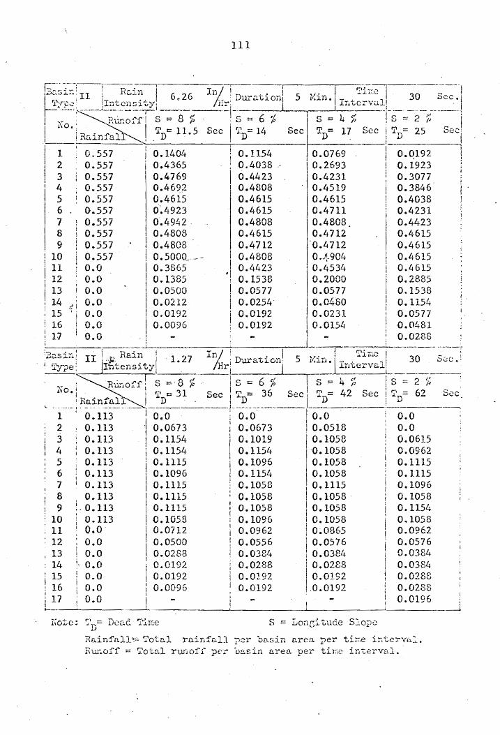
III
,..--_~w_.~ __ : ___ ._"'_..-! ___ _
Ip32<SlY:' II ! R[;"ln I 6 26 In% \ D =~-=-I 5 ~~; n.. ?'r;.e i-'-;-o--~(;C .-'1' rl:"'r'~'" IT"~·"'->1~·~.Ly .. ) --, Ul""IJ10UI .... -""- 11
.. u,.;, t ...... ,,~. ~ .... v I .t1r, ~ ... _~crvo. ___ J,_-_~, ,._. ________ ' ,I
-'~-"'<'--~-'~~-;~'~:~~~~T'~- = 8 % ,-I-~-_-6-%.....o.----r--S-=--'·~4-~; "8-=-2---,; - I'
i\.-0 ' • w. .l. I I oJ - ~ I h .. ; R~'; .(' '1 Tnt:: 11.5 Sec lTD:':': 14 Sec TD= 17 Sec! 'I'D= 25 secl~ I l .. u...t...n ... a..l.. I. I
I -: i 1 0 . 557 0 .. 1404 0 .. 1154 0 to 0769 I 0 • q 192 I
i 2 0.557 0.4365 0.4038 10.2693 I 0.1923 . I 3 0.557 0.4769 0.4423 I 0.4231 : 0.3077
I, 4 0.557 0.46~,2 0.4808 0.4519 0.3846
0.557 O~4923 0.4615 0.4711 0.4231
I'
57: 0.557 0.4615 0.4615 0.4615 0.4038
0.557 0~4942 ' 0.4808 0.4808 0.4423 0.557 0.4808 0.4615 0.4712 0.4615 I I ! 9 0.557 I 0.4808 0.4712 '0.4712 0.4615
10 0.557 I O.5000~_,~- I 0.4808 0 .. 1:-904 0.4615 11 0 .. 0 i 0 .. 3865 I 0,,4423 0.4534 0 .. 4615 12 0.0 " 0.1385 "I 0 .. 1538 0.2000 0.2885 13 0 .. 0 0.0500 I 0.0577 0.0577 0.1538 14 :11 0.0 I 0.0212 I 0.0254 10 .. 0480 0.1154 15 " 0.0 I' 0.0192 i 0.0192 10.0231 0.0577 16 0.0 0.0096 0.0192 0.0154 0.0481 17 0.0 ! I 0.0288
_._.,L~__ ' ,I ___ . _____ ,n __ ~
... '1':-' a on 5 1l-i -,I. .! 30 S(;;C .; ,::3uSi:.i.1
,f II' i ,,'.'" Rain II '1.27 1% 1" D ..... t,-' I Tir.e I j • I "", .... -. i \,.U. ..L .. : ---. -.l'YJ.+C":"'\"~! 1 I, 'l.Y?e: Itrtensl tY j .t1ri ____ ~I_-. __ ____...._· _v_-_-_-L _______ _
, . -f' S 8 d It S - 6 q I s - 4 ,f 1 S - 2 'I' v! Rur.Ol'· t:: '};- . - 1(1 I - /: 'j - J
t;O·l ' : T c 31 Sec I? = 36 Sec II T = 42 Sec .,li Tn= 62 Sec : Rainfal.t I D '. I D D
-... -, - _. ".'.'-- -"----_' • --_........-____ .l~ ------------ ---- ----------
1 · 0.113 I 0.0 ! 0.0 10.0 ' 2 0.113 0.0673 0.0673 I 0.0518 j 0.113 0.1154 O~ 1019 ! 0.1058 4 0.113 0.1154 0.1154 1'0.1058 5 0.113 0.1115 0.1096 10.1058 6 0.113 0.1096 0.1154 I 0.1058 7 0.113 0.1115 0.1058 I 0.1115 8 0.113 0.1115 0.1058: 0.1058 9 1. 0.113 0.1115 0.1058 I 0.1058
10 0.113 0.1058 0.1096 i 0.1058 . 11 0.0' 0.0112 0.0962! 0.0865
12 0.0 0 .. 0500 0.0556 I 0.0576 13 ! 0.0 0.0288 0.0384 t 0.0384 14 1, 0.0 0.0192 0.0288 I 0.0288 15 ! 0.0 0.0192 0.0192,' 0.0192 16 0.0 0.0096 0.0192 .0.0192 17 0 .. 0
i~otc: ~1D;:; Dead Tirr.:e S = LODGi tude Slope
0.0 0.0 0.0615 0.0962 0.1115 0.1115 0.1096 0.1058 0.1154 0 .. 1058 0 .. 0962 0.0576 0.0384 0.0384 0.0288 0.0238 0.0196
Ra.infall::=- ?otal rninf£:.ll ller bnsin area per ti:;-,e iDtcrvil.l. Rur .. off :::: Total runoff peT oas in urea. per tiro"le intervD.l.·

1 2 3 4 5 6 7 8 9
10 I 11 I I 12 I 13., I 14 i~ ! 15
1.250 1.250 1.250
'1.250 1.250 1.250 1.250 1.250 1.250 1.250 0.0 0.0 0.0 0.0 0.0
1]2
6 • 2 (, 5 }O; in.
0.5769 1.1154 1.1346 1.09.62 1.0769 1.1346 1.0769 1:1346
.1.0769 1.1154 O~ 7-115
IS:::: S :::: I ? :::: 12 Sec
D
0.5000· 1. 1154
'1.0962 1.0577 1.0962 1.1346 1.076.9 1.1154 1.0962 1.1154 0.6731 0.1154 0.{)385
. '3;'.5 i r. i II I !_'iE\~i ~ ,I I 1. 2 6 I~ ~ 'II D'~ a\:. i C;:l! 5 ~r.i n./ ..1.-"" .... ne~ ~ -v''': i
30·
S :::: 2 /~
':::J==- 18
0.3846 1. 1538 1.0962 1.0577 1.0962 1.0962 1.0769 1..0769 1.0577 1.1346 0.7885 0.2115 0.0577 0.0288 0.0192
30 ~ r:::y;?e 1 i.Lr/cei.;'s:!:c,y: lH:t': I ! ~.l v ... .-:.. ....
'-. -~ ~",i 81 8 d ,-... --I"-d-.-L---11'""-S--'--ll-d--"':-S-- 2 c;'
: Xo.! ~lOI 1 I ':i!D=' 2/J
.' Sec l! .~_.L_:'\: ~o~ 5 Sec! T_:;6 /# Sec '.i.'D= 47 .• /~ ~ . ';;;>,..,.: -:-"", 1'~ ! J.,I! J.)
-~ -.-!~-=::~~~:.~-:::--~ 1 · 0.252 .i 0.0096- ;' 0.'0 I'
2 0.252 J 0.1827· 0.1427
: g:~;~ I g:;zg~ g:;;gci I· 5 0.252 . I .0.2212 0.2212·-j
. 6 O. 252 I O. 2212 O. 2500 I 7 0.252 L 0.2212 0.2308-8 0.252 i '0.2212 0.2308 - ! 9 0.252 .1 0.2212, 0.2308!
10 0 .. 252 I 0 ~ 2308 0 . 2404 i t I -
II 0.0 1 0.1731 0.1827! 12 0.0 0.0577 0.0481 i
13 0.0 0.0385 0.0288! 14 0.0 0.0192 0.0192 I.
0.0 O. 1346 o. 240~· 0.2500 0.2491 0.2404 0.2308 0.2308 0.2308 0.2308 0.1635 0.0673 0.0385 0.0192
0.0 0.0577 0.2404 0.2404 0.2404 0.2404 0.2308 0.2404 0.2115 0.2404 0.1827 0.0673 0.0345 .0.0192
~ - .... : ... 1\;: .... .o:
I ! --------------~----------__ ~ __________ ~! ___________ ~ _________ __1
:i~ir.:.~[!..lj.;= '::ot~D.J_ rui:lfnll. !?0r be:..si:l area, p-e:- ti:7A2 ir:~c~,r[;.:L.
Rw.1oi";. ... p 70tal :rl..:.."'loff J!cr basi;."! areu. per tiri,C ir..l.tcl·val.

) ] 3
1'3~.~~ n :---i---R~i-~-I!-------Il%J I:-~--l--,!--.-I---'l\';' r;.'~-j--- -----s- ~--I I I I - . I 0 8') _¥, J.Ju:z:'3.l.10nj t: t.lD.' - I 30 ce.' I lJ. .... T02; :.lntc::1sJ..:cy\ • ,.) Hr,::> I .In't~ervull , i
~~ -. N' .: ." ~---::-r-S- - 8 d l-S - 6 r/ - c' -' 4 cI i-;-~-2-("----~I'
'X O. I h uri. 01.1. r '- 7~ i-Iii ..., - /1) j .::.> - /0 . . I I rOIJ.. .- Sec I r.1.l - Sr.·c r:\ - ~e.-. I M.l - Sc~cl
I R ~ .r 1 '- ~ D~ 4ft I D- 53 '- .t'D- 60, ..., - : D- 87 '- I I" U.LnJ.a l._~i . I i
',! I' I I IIi 0 .. 164 'I· 0 • 0 I 0 • 0 o. 0 I o. 0 I I 2: 01} 164 0.,0327 I 0.0135 0.0 1 0.0 I
3 0.164 : 0.1404 I 000827 ' ;0.0673 1 0.0019 I 4 ~6 I 1 I 046 ' Dol it ! O.14l!2 ,0.1346 0.058 I O. 9 i 5 O~ 161+ j 0$1442 0.1346 0.1255 j 0.0962
'6 0.164 ! 0.1442 0.1538 0.1255 ! 0.1250 7 0.164 ! 0.1442 0.1269 0.1269 1 0.1346 I : 8 00164 i Oc1538, 0.1423 0.1346· I 0.1346 9 0.164 i 0 ... 1346 0.1423 0.1442 I 0.1423
10 0~164 I 0.1538 0.14l~6 0.1442 I 0.1442 11 O~O I 0.1154 0.1250 0 .. 1269 j 0.1346 12 0.0 0.0481 0.0577 0.0769 I,i 0.1005 13 ~ 0.0 0.0385 0.0385 i 0.9480 I 0.0679 14 000 I 0.0288 0.0288 I 0 .. 0364 ! 0 .. 0481 15 0" 0 I 0 .. 0192 0 " 0192 I' 0 .. 0201 O. 0357 16 0.0 0.0100 0.0100 0.0120' 0.0288 17 0.0 ji, _~l . ' I i 0 .. 0192 .. __ ,
.':ac.sin 1 ! Rain i In/ I . 1- ,. I ?irr.e i ; ~ T'.1pe!III JIntensity! 0.83 /Hri Duratl.Onl 5 ~an. i Intervali 30 Sec.:
~! RUnoff'! S :::,8 % Is t:: 6 % II' S::: 4 % ,is;;: 2%---" j ~~O. I iii l I Rainfo.1J. 1 TDc 36 Sec: T ::: 42 Sec I TD::::: 1~9 Sec: ?D= 64 Sec ~_. ___ . __ , ____ I~_? ' L _____ .J; ______ --,
I I I i 1 0.164 0.0 O.O! OcO 0.0 2 0.164 0.0769 0.0385 I 0.0269 0 .. 0 3 0.164 0.1250 0.1154,' 0.1077 0.,0865 4 0 .. 164 0.1538 0.1442' 0.1347 C . 14l.2
, , 5 0.164 0.1538 0.1442 I 0.1538, 0.1442 6 0.164 0.1538 0.1538 I 0.1538 0.1442 7 0.164 0.1346 0.1346 i 0.1346 0.1442 8 0.164 0 .. 1538 0 0 1442 I O~1442 0.1635 9 0 .. 164 0.1442 0.1442 i 0.1442 0.1538
10 0 .. 164 0.1442 0.1538 I' 0.1538 Oc1442 11 0.0 0.1154 0.1154 0.1154 0.1250 12 0.0 Oc0385 0.0576' 0.0576 0.0673
I 13 0.0 0.0211 0.0215 II 0.0288 0.0318 14 0 0 0 0.0192 0.0192 O~0195 0.0211 15 0.0 O~0100 0.0100 I 0.0100 0.0100 16 Q.O 0.0851 0.0851 /' 0.0851 0.0962
Note: T :: Dcad Time D
S = Longitude Slope
Ruinfall~ Total rainfall per basin area per tiwe intcrv~l. Runoff = ?otal runo~f per basin urea per time interval.'

1 2 3 4 5 6 7 8 9
10 11
l 12
I ! I i
J '!
0.12G 0.126 0 ... 126 0.0 0.0 0.0 0,,0 0.0 0.0 0.0 0.0
1% j If," I Ti-::-.c I, -, ! ~".".....,tion 1 ~.~n -1-' 11 15 Sec_\ .. ,u.............. !, .In'tcY'VD. i :
Jirj! i---- _~_. ___ ! ~s:::6% II s=4/~ IS=2i~ !
Sec ,'TD= 29 Sec I 'I'D= 37 Sec! T ::: 45 Sec ! D I ! I i
I o. 0 II o. 0 O. -0 I 1 0.002 0.0 0.0 i II 0 . 040 0 . 017 O. 0 { .
0.093 0.067, 0.013
II 0 .. 101 O. 117 0 .. 042
0.068 0.073 0.091 0.025 0.037 0.090
I, 0.013 0.019 0.064 0.007 0.012 0.021
I 0.004 It 0.005 0.010 0.014 0.003 0.003 I 0.006 0.008 0.003 ! 0.003 I 0.003 0.006
I I I I I I I ! i ~ _________ ,
,:33.sin I "~~'R~i;-~ I 1%' i I .... ,. I Tir.,e! , II.L OJ I H' r! Di.ll"'E:.tion, l'f'.::Ln. \' I' .,! r;."JPc j nl.,.ens:u~YI n-cervaJ.j S.::c .. '
Runoff'! S :::' 8 ;; ! S ::: 6 % .... tV
,.........----...:--"-------r- S = 1" ¢,'{I .Ii S--~·-2-S~--~:
:-: o • 'I T t:: Sec ! T ::: ' Sec I T = Sec 'I ?D= Sec~. t----- Rnin_~!:,~~-.E_-'_, _' __ L_~ ________ D _____ i _____ _
j I I
II I I
I I
I i ,I j
j 1 L~~ __ ~ ___ ~ ____ ~ __ ~ __ __
S = Longitude Slo~e
~ainfall~ Total rainfall per basin area Ru."1.off = Total runoff per basin urea per
per time interv~l. tir,',C! interval.'

1] 5
I'B~·; in I~--~r -----R~-i n-~I---6--? h - ~I-%-' -r D-Ul-~"'" -4. ·i o~ l-l~'--:::n l-- --~l-j ~.2 --3-0--------
tl1.,rn; ,'I L • t r () ._v H ~; I u, '-'- J.~! \" .'l.l 'J' I'''' Sec f ,
........ J._J .r::~: __________ "::_::":~ Sl sJ____ ____ r, ---.l n-cerva.L'
jl No.1 . .Runoff'l S :::: 8 % ----II-S~~-6-1; =l-~s--~ 4~;-----';-S--'-2-~;
l' . rr:::: 14 Sec 16 Sec 1.1 :::: 17 Sec: rr := 26.5 Sec
_~_ Ralnfal__ D I D : D
I 1 I 1.25 Ii 0.2835 I 0.2308 I 0.1923 1---0:.0192-i
I
2 I 1.25 1.1154 I 009808 0&9231 0.5000 3 I 1.25 I 1.1538 I 1.1346 1.0769 0.8654 4 I 1.25 I 1.1731 I 1.1538 1.1731 0.9808 5 I 1.25 1.1660 1.1538 1.1731 1.0577 6! 1.25 - 1.1635 1.1731 1.1923 1.1154 7 II 1.25 1.1538 1.1346 1.17~1 1.1346
I
8 1.25 1.1731 1.1538 1.2115 1.1538 9 i 1.25 1.1731~--- 1.1731 1.1731 1 .. 1538
10 l 1.25 1.1731 1.1731 1.1923 1.1731 11 I 1.25 1.1538 1.1538 1.1923 1 0 1731 12 i 1.25 1.1538 1.1731 1.1923 1.1923 13 14 1.25 1.1923 1.1538 1.1923 1.1538 14 I 1.25 1.1538 1,,1538 L.1923 1.1731 15 I 1 .. 25 1.1538 L.1731 1 .. 2115 I .. 1538 16 I- 1 .. 25 1.1538 1.1731 1.1731 1.1731 17, 1.25 r 1.1538 1.1538 1.1731 1.1538 18 I 1.25 1.15:,8 1.1538 1.1538 1.1731 19- I 1.25 1. 1731 1. 1731 1. 1731 1. 1538 I - I 20 1.25 1.1346 1.1731 ,I 1.2115 l.l731 21 I 0.0 0.9038 0.0423 0.9423 1.0577 22 i 0.0 0.2308 0.3077 I' 0.4423 0.7692 23, 0.0 0.0577 0.0577 I' 0.0962 0.4038 24 II 0.0 0.0384 0.0385 0.0577 0.1538 25 0.0 0.0254 0.0254 I 0.0385 0.0769 26, 0.0 0.0192 0.0192 I 0.0192 0.0384 27 I 0.0 I 0.0385
I I I ,I
I.
I I
I I I JI I I !
, _____ -l... _____ -L_________ ._
Note: TD:::: Dead Time S :::: LonGitude Slope
Rainntll~ Total rainfall per basin area per time interval. RUL"1off ::: Toto.l runoff per basin f.rea. per tiree interval.

1]6
iB;.si~r---I-- --r- -Rcd~l'- j- -1 ?6-fu/ ! D~-~~-~~~f--l-0-;inJ-~irr.e-r---~-O' --- S~-c ~: 0!E~_~ ___ E~t_~nS~~!"I __ "_-___ i~~i_~u ____ ~~_ I In~~rvaJl ~ ____ _ 1 "I Runoff S::: 8 % !, s ::: 6 % IS::: 4 5~ ! s ::: 2 % !
I No. ITt.:: S ~ T - S rn ::: Sec I '1' ::: Sec I R .: f 1 I D 34 e..... I n- 1.1 ec J.. D 47 I D I ,a.Ln ai' 'I .- ._-_._-.--! 1 I I' I I 0.252 0.0 0.0 0.0 I
I '
2 I 0.252 0.0769 it 0.0502 0.0288 1
3 I 0.252 0.2308 0.2212 0.1635: 4! 0 0 252 0.2500 I 0.2212 0.2115 5 I 0.252 0.2500 0.2308 0.2404 6 0.252 0.2500 0.2308 0.2115 7 0.252 0.2500 0.2212 0.2115 8 0.252 0.2500 0.2404 0.2115 9 0.252 0.2500 0.2212 0.2115
10 0.252 0.2500 0.2212 0.2125 11 0.252 0.2500_ 0.2212 0.2212 12 0.252 0.2500 0.2308 0.2212 13 Q.252 0.2500 0.2212 0.2115 14 0.252 0.2415 0.2212 0.2308 15 0.252 0.2500 0.2212 0.2500 16 I~ 0.252 0.2510 0.2212 0.2410 17 0.252 0.2417 0.2115 0.2212 18 0.252 0.2500 0.2115 .0.2212 19 0.252 0.2500 0.2115 0.2212 20 0.25~· 0.2612 0 .. 2212 II. 0.2404 21 0 0.1923 0.1923 0.2115 22 0 0.0769 0.0673! 0.0865 23 0 0.0385 0.0385 0.0481 24 0 0.03B5 0.0288 0.0385 25 0 0.0192 0.0211 0.0288
Note: TD
:::. Dep.d 'l'ime S ::: Longitude Slope
Rainfall-;=: Total rainfall per basin arca per tir::e intcrvaJ... Runoff::: Total runoff per -Dasin area per tiif:-:': interval ..

1 2 3 4 i 5 I
I 6
I 7 8 i
: 9 i
10 I 11 I,
12 13 ! 14- I 15 t 16
f 17 18 19 I 20 ~
21 I I
22 I
23
I 24 25 1 26 I
I
27 I I I
I I I
I I I
i
1]7
'I'irr:':8 - -- ---- ------- ----·1
0.83 10 Ivan. 30 Sec. :
8 % S ::: 6 rl S = 4 t:f ----;,-- -----1
== Ie /0 S ::: 2 I'} j
T t= 43 Sec T ::= 50 Sec 63 Sec TD= 85 Sec' D D
O.16f} 0.0 O.Q 0.0 0 .• 0 0.164 0.0481 0.0195 0.0 0.0 o • 16ft 0.14/-f2 0.0901 0.0500 0.0071 0.164 O.ll~42 0.1346 0.1135 0.0987 0.164 0.1500 0.1538 0.1346 0.1250 0.164 0.1481 0.14l~2 0.1250 0.1442 0.164 0.14[1-2 0.1250 0.1250 0.1250 0.164 0.1442 0.1442 0.1346 0.1346 00164 0.1442 0.1442 0.1346 0.1442 0.164 ~ 0.1442 0.1346 0.1346 0.1442 0,,164 0.1538 0.1442 0~1538 0.141.-2 0.164 o. 14~ :r-----
i 0.1442 0.1442 0.1346 0.164 0.1538 I ' 0.1442 0 0 1442 0.1538 0.164- 0.14li-2 I 0.1442 0.1250 0.1250 0.16l~ 0.1442 I 0.1346 0.1538 0.1346 0.16/-+ 0.1442 ! 0.14l;.2 0.13/.6 0.1.442 0.164 0.1442 0.,131:6 o .llt42 0.13l+6 0.164 o .1lrl~ 2 0.1538 _ 0 .. 1346 o. ll~I~2 0.164 o .14l t2 0.1346 0.1250 0.1346
O01E~ 0.1442 0.1538 - 0 .. 1442 O.14l~2
0.1346 0.1250 0.1250 0.1346 0.0 0.0 0 .. 0577 0,,0587 0,0673 0.1024 0.0 0.0231 0.0288 0.0480 0.0587 0,,0 0.0154 0.0192 000481 0.0481 O~O 0.0087 0.0096 0",0192 0.0288 0,,0 0.,0076 0.0288 0.0 0 0 0192
!
S ::: Longitude Slope
Rainfall-;=: Total rainfall per basin a.rea. per time interval. Runoff::: Total runoff per basin area per tin~e interval.

118
IBC~i~-~~jl ----R;i?-l-l--:;~-in/ r;~~-~~:Orr1~-~~i~~]----Tf~c ~ ;-- ;-0 ---- Sec. ' 1 'PIpe ___ Intens~L_' L ____ ~!:j _______ r _ _,.___ Inter~a.LL
I, T I RUnoff S::: 8 % j S ::: 6 ,; l' S ::: 4 % : S =: 2 ,; i
No. !. I' T = 30 Sec! T = 37 Sec T::: 42 Sec: T = 60 Sec .1 t RUlnfal D D _ D ___ D_._. ________ _
II 1 1 0.113 0.0 0.0 I, 0 .. 0 0.0
2 0.113 0.0673 0.0577. 0.0510 0.0 3 0.113 0.1154 0.1154 0.1154 0.0769
II 4 0.113 0.1058 0.1154 0.1096 0.1058
5 0.113 0.1054 0.0962 0.1154 0.1154 I 6 0.113 0.1154 0.1154 0.1096 0.1096 I 7 0.113 0.1154 0.0962 0.1115 0.1115
I 8 .0.113 0.1154 0.1058 0.1154 0.1154 9 0.113 0.1115 0.1058 0.1115 0.1058
; 10 0.113 0.1096 0.1058 0.1096 0.1154 11 0.113 0.1115 0.1058 0.1058 0.1058 12 0.113 0.1058- 0.1058 0.1058 0.1115 13 0.113 0.1058 0.1058 0.1154 0.1096 14 I 0.113 0.1058 0.1058 0.1058 0 .. 1115 15 1 0.113 0.1058 0.1115 0.1058 0.1115 16 0.113 0.1058 0.1058 0.1058 0.1154 17 -1 0.113 0.1058 0.1115 0.1058 0.1154 18 . 0.113 0.105~ 0.1058 I 0.1058 0.1058 19 0.113 -0.1058 0.1058 I 0.1115 0.1058 20 0.113 0.0962 0.0962 0.1115 0.1115 21 : 0.0 ~;;, 0.0673 0.0865 1_ 0.0962 0.0962 22 I 0.0 0.0481 0.0481 0.0577 0.0769 23 1 0.0 0.0288 0.0288 0.0288 0.0384
I I 24 ! 0.0 0.0192 0.0194 I 0.0194 0.0288 25 I 0.0 I 0.0154 0.0192
1 I ! I
I I
I ... ------'--------'-----___ --'_~ ____ ___1 ______ ____"__ ___ -- ._--
Note: TD= Dead Tirne S = Longitude Slope
Rainfall~ Total rainfall per basin firea per ti~e intcry~l. Runoff:: 'rota.l runoff pe:!:" basin area per tire interval.

119
,- . -1- ---,.- --- - ----T------- -- ~-.--. _._--... ---,.---:Basin J Rain I 1% ~ . i . ~I ~ I II I t 't 6,,26 If D1U
1
ut).Olll 10 M~n J.JP2 1 n cns~ y' r,
30
, I
Sec: 1·~--I--·~::-f-~~-·~-~·8· %----J-S-= -6%--'-----.-·S----:::-.L-4- 5-{---- S ::: 2 %
I .t.O·!R· f 1 ! Tn:::: 12.5 Sec Tn= l lt Sec T = 16 Sec T:::: 24 l- a~n a , D D
I; -1-1··O~557-·1 0.1346 i--:-0.1154----1--0-,,-0--8-65---:··· 0.0-2-'-3-1----
2 ! 0.557' I 0 .. 4615 i 0.4038 0 .. 2981- 0.'1885 I 3 I' 0.557 I 0.4423 0.4423 0.4231 0.2981 1'4 0.557 1 Oc4808 0.4615 0.4423 0 .. 3942
I 5 j 0.557 0.4615 0.4615 0.4615 0.4231 6 I 0.557 0.4423 0.4615 0.4615 0.4231
! 7 I 0.557 0.5000 0.4615 0.4712 0.4/+23
I
8 I 0.557 0.4808 0.4808 0.4712 0 .. 4712 j' 9 I O.S57. 0..1 .. 615 0 .. 461S· 0.4808 0.4519 I 10 : 0.S57 0.4615 0 .. 4615 0.4615 0 .. 4712
I, 11 I 0.557 0.4712. 0.4615 0.4808 0.4712
12 1 0.557 0.5096 .0.4615 0.41l-24 0.4808 ! 13 I 0.557 i 0 .. 4808 0.4808 0.4808 0.4808 I 14 I 0.S57 I 0.5000 0 .. 4615 0 .. 5000 0.4904 ; 15 ~ 0.557 I' 0.4808 0.4808 0.4615 0.4615
16 0.557 I 0.4615 0.4615 0.4615 0.4712 17 0.557 0.4808 0.4615 0.4808 0.4712
~-18 0.557 i 0.4808 0.4615 0.4808 0.4808 19 0.557 I 0,,4~08 0.4615 i 0',,5000 0.4808 20 O.551f' I' 0.4615 0.4615 I 0.4615 0.4519 21 0.0 0.3462 0.4423 0.4423 0.4615 22 0.0 0.1250 0.1154 I' 0.2308 0.3269 23 0.0 I 0.0346 0.0384 I 0.0769 0.2308 24 O.Oi I 0.0340 0.0340 0.0385 0.1538 25 0.0 0.0192 0.0192 0.0192 0.0962 26 0.0 0.0115 0.0192 0.0603
r
27 0.0 I 0.0451
28 0.0 I I 0.0200
I
I I
lioie: Tn== Dead Time S == Longitude Slope
Rainfall~Totnl rainfall per basin area per ti~e intc~val. Runoff :;:: Total runoff per bas in area per tir!:e interval.

]20
,--tj}::;C"in i <.,.., 'Ill !3r pe l
Durati 10 30 Sec.
! ; I No. i RUnoff I _L _____ rainral ! I ; i11.250 i I '
I 2 I 1.250 I 3 ! 1.250
4 I 1.250 5 II 1.250 6 1.250 7 I 1.250 8 ! 1.250 9 I 1.250
10 I 1.250 11 Ii 1.250 12 1.250 13 1.250 14 I~' 1.250 15 I 1.250 16 1 1.250 1·7 ! 1.250 18 1" 25~J.;' 19 1, 25fJ' . 20 1.250 21 0.0 22 0.0 23 0.0 2l.. 0 .. 0 25 0.0
! i i I I i
li I
Sec
1.0769 1.0577 1.0577 1.1154 1.0962 1.0769 1.0769 1.0673 -- -1.0865 1.0769 1.0577 1.0769 1.0577 1.0769 1.0577 1.05~7 1.0769 1.0769 0.6154 0.0962 0.0385 0.0192 0.0096
Hote: T ::: Dead Time D
s == 6 % 11.5
1.0673 1.0865 1.0769 1.1154 1.0769 1.0962 1.0769
! 1.0962 i" 1.0769
I 1.0962
I 1.0962 1.0769
I 1.0962 I 1.1154 i 1.0769 I 1 1.0962
1.0769 1.0962 0.6923 0.1154
! 0.0385 I I 0.0192 i 0.0096 I I i I
I
I I I I
I I I i
13.5Sec
0.5000 1.1154 1.0962 1.0962 1.0769 1.1154 !'.O7l?9 1.0962 1.1154 1.0962 1.0962
I !
1.0769 1.0962 1.0962
I I
1.0769 1.0769-1.0577
i 1.0769 I 1
I I r I
1.0577 1.0769 0.7500 0.1250 0.0385
I
i 0.0192 0.0096
I
i J
I
I
I S = Longitude Slope
S ;:;: 2 r-.' Iq
T :::: D
19
0.3462 1.-1346 1.0769 1.0962 1.0577 1.1154 1.0576 1.0577 1.0769 1.0577 1.0769 1.0769 1.0577 1.0962 1.0962 1 .. 0577 1.0577
i 1 .. 0962
I 1.0769 I
1.0769 0.7500 0.1923 0.0577 0.0288 0.0145
Rainfa11= Total rainfllll per basin area per tir..e intcrYH.~.
Ru..T10ff ;:;: Total runoff per casin area per tin:e interv31.
Sec
I

-- 1'-"-- ---r---: I Rain , ITT;
"-- Intens
2 3 4 5 6 7 8 9
10 11 12 , 13 I
I ~~ ~ 16 1
1
17 ! 18 19 20 21 22 23 24 25
0 .. 252 0.252 0.252 0.252 0 .. 252 0.252 0 .. 252
-0.252 0.252 0.252 0 .. 252 0.252 Of;252 0.252 01'252 0.252 0 .. 252 0.252 O.25~ 0.251 0.0 0.0 0.0 0.0 0.0
0.0096 0.1731 0.2308 0.2212
-0.2212 0.2212 0.2308 0.2115 0.2212 0.2212 O.240i! 002212 0.2212 0.2212 0 .. 2212 0.2115 0 .. 2115 0.2212 0.2212 0.2303 0.1634 0.0385 0 .. 0193 0.0096 0.0096
] 21
0.0 0.1427 0.2404 0.2404 0.2404 0.2500 0.2212 0.240l. 0.2308 0.2308 0 .. 2308
... 0.2500 0.2308 0 .. 2308 0.2308 0.24-04 0.2308 0.2308 0.2308 0 .. 2404 0.1635 0.0577 0.0193 0.0096 0.0096
10 f.lin.
Sec s == T ==
D
0.0 0.0865 0.2212 0.2500 0.2404 0.2115 0~2308
0.2308 0.2308 0.2308 0.2212 0.2308 0.2212 0,,2212 0.2212 0.2308 .
·1 ~: ~;~~ . I 0.2212
I
I 0.2212 _ 0,,1827
0.0865
I 0.0193 0.0096 I 0.0096
I I
I I
i I I I 1 I
. I I L __ ~ _____ -----L ______ L.....-.-______ 1--_
Note: Tn= Dead Time S == LonGitude Slope
30 Set;.
47 E'2C
0.0. 0.0673 0.2500 0.2692 0.2308 0.2500 0.2500 0.2308 0.2302 O .. 23CD 0.2404 0.2500 0 .. 2308 0.2308 0.2308 0.2404 0.2308 0.240/+ 0.240!:· 0.2308 0.1923 0.0769 0.01.93 0.0193 0.0096
Rainfall-:;=: Tota.l rainfall per bn.sin area per tirr;e intcrv.:..:. RU.110ff = Total runoff per bas in area per tirr,e interval.

122
r::['B:~i~r~;;lI--~-Rai~t---I- o. 83 --i~/H--r~tll::::~~~rl: 10 Mi~}-I--~~~l~-r.;~ll-.. -··-;-o Sec.
I ~:pek--L~~:;i!~ = 8 % -~!:I S = 6 % - I S ~14ni~~'1=-I-s = 2-
I ,'0. i Rai:s. i TD'" 37.5 Sec I TD= 42.5 Sec Tn= 48 Sec i "'D= ft, Sec'
~_I 0.164 ~o I 0.0 0.0----- -- 0.0,
2 0.164 0.0481 i 0.0346 0.0288 0.0 3 0.164 0.1058 1 0.1154 0.1058 0.0865 4 0.164 0.1538 0.1384 0.1442 0.1346 5 0.164 0.1538 0.1538 0.1538 0.1538 6 0.164 0.1442 0.1442 0.1538 0.1442 7 0.164 0.1538 0.1442 0.1442 0.1442 8 0.164 001442 0 .. 144·2 0.1442 0.1538 9 0 .. 164 0.1442 I 0.14L~2 0.1442 O.14!t2
10 0.164 O.14L:·2 I 0.1442 0.1442 001442 11 0 .. 164 0.1442 " O .. 14b.2 O.141i-2 0.1442 12 i 0.164 0 .. 1538 0.1538 O.14tl2 0 .. 1538 13 ! 0.164 0.14L~3 0 .. 1443 0.1443 0.1443
I
14 r 0.164 0.1351 0.1442 0.1351 0.14L~2 15 0.164 0.1442 0.1442 0.1LI'.2 0.1351 16· 0.16!f 0.1442 0.1442 O.14l1-2 0.1346 17 0.164 001442 0.1480 O,,14L!>2 0.1500 18 Oc164 0.1442 0.1405 0.1380 0.1331 19 0.164f"· . 0 .. 1530 0.1442 0.1500 0".1442 20 0.164 0.1442 0.1442 -I 0.1442 0.1530 21 0.0 0.1250 0.1346 I. 0 .. 1346 0 .. 1250 22 0.0 0.0385 0.0385 I 0.0481 0.0553 23 0.0 0.0192 0.0192 0.0288 0.0198 24 0.0 0.0096 0.0115 0.0192 0.0192 24 0.0 0.0077 0.0096 0.0096
Note!
--'---- ---.-
Dead Time S = Longitude Slope
Rainfall Total rainfall per basin a.ren per tirr:8 inte:cv.?k~."
RWl.off = Total TtU10ff per bas in £.rea per time i 1':. tcrval.

123
!B~.l.·-y~-~;i-;---Jf.L~-t~ri~il.lt T~;6 i~?I:;tU~;;~:r~;-- g-~-~-:r, ~~T{rr.;-~-l,~-----;o SE:C.:
r .P~! __ ~~~;l. yl _______ /~I:L__ I ..Ln"ccrva.L:
No.1 Ru.nOr-r: s ~ 8 % IS" 6 % I s =L4 %~---TS--~-2-1; , I Rainfal I TD= 13 Sec TD= 15 Sec 'lID=17.5 Sec I rfn= 26 SE:C
-~---!----- I -.1--------------, 1 I 1.250 i 0.3462 0.3269 0.1731 I 0.0192
i i ! i , I l
2 I 1 .. 250 I 1.0769 0.9808 0.9231 t O~5000 3, 1.250 I 1.1731 1.0577 1.0962 I 0.8846 4 I 1.250 I 1",1346 1.1346 1.1538 I 1.0000 5 I 1.250 I 1 0 1923 1.1538 1.1538 II 1.0577 6! 1.250 : 101731 1.1538 1.1538 1.0769 7 1.250 - I 1.1346 1.1538 1.1731 I 1.1538 8 I 1.250 ~ 1.1731 1,,1538 1.1538 i 1.2115 91 1.250 ! 1e1731~ __ - 1.1538 1.1538; 1.0385
10 I 1.250 1.134-6 1.1538 1.1731 1 1.1538 11 1.,250 Ii 1.,1538 ' 1.1346 1.1731 i 1.153S 12 I 1.250 I 1.1731 1.1923 1.1538 i 1 .. 1538 131!~1 1.250 ! 1.0769 1.1731. 1.2115 1.1538 14 1~250 I 1.1346 1.1731 I 1.1538 1.1538 15 1.250 i 1.1923 1.1731 1.1731 1.1538 16. I 1.250 II 1~1538 1 .. 1911 I 1.1538 1 .. 1538 17 I 1.250 1.244-5 1.1538 1.1731 1.1923 IS! 1.250)' I 1. 2013 1 .. 1731 I 1" 17311. 1731 19 i 1.250 I 1.1)31 1 .. 1923 1.1923 1.1538 20 I 1.250 I 1~.1731 1.2115! 1.1923 1.1923 21 I 1.250 I 1.1923 1'.1346 I 1.1347 1.1923 22 i 1.250 I 1.1731 1.1538 I- 1.1923 1.1539
;~ I i:~~g I:.: ~:i~~~ i:i~~; I i:i;~~ i:i;;~ 25 l 1.250 1 .. 1538 1.1731 i 102115 1.1731 26! 1.250 1,,1731 1.1923 I 1.1346 1.2307 21\ 1.250 1.1538 1.1538 I 1.1131 1.1538 28 I 1.250 1.1731 1.1923' I 1.153~ 1.1731 29 I 1.250 1.1731 1.1923 i 1.1538 1.1538 30 I 1.250 1.0981 1.2307! 1.1923 1.1538 31 0 0.9138 0.9808! 0.9615 1.0385 32 !, 0 0.3208 0.3315 0.4231 0.7301 33 I 0 I 0 • 0577 0 • 0769 0 .. 0962 0 • 3846 34 : 0 \' 0.0384 0.0384 0.0384 0.1538 -35 i 0 I 0.0336 0.0336 0 .. 0336 0.0769 36 : 0 O. 0192 0 • 0192 0 • 0 19 2 0 • 0384
I I
I I I L __________ ~ __________ L_ ________ ~ __ _
Note: Tn= Dead Time S = LonGitude Slope
Rainfall~ Total rainfall per basin area per ti~e intcrv~l. -Rll.'1off := Total runoff per basin arca per tirne interval.

F~~~;-!~~J~~~~ ~J-_~-~~~ I%rF~~~O~r~~I~~:'t~~~~[~~=~~_~C~~ I -~ I Rlh'1off: S::: 8 % is::: 6 % Is::: 4 % " S ::= 2 % j
L J,.o·1 T :::: 35 Sec j 'I'D::: 40 Sec I' TD:::: 47 Sec lTD::: 64 Sec 'j ___ t_~~ip:fal_~. __ D ____ -+I _______ · .. :. ______ _ I 1 'I' 0 .. 252 0 .. 0 I 0.0 I 0 • 0 0.0
2 I 0.252 0.0769 0.0498 0.0288 0.0
~
;
.
j
I , I I ! I
3 i 0 .. 252 0.2115 I 0 .. 1635 0.0567 4 I 0.252 0.4423 0.2308 I 0.2115 0.1332 5 i 0.252 0.2115 0.2212 0.1705 6 I O~252 0 .. 4904 0 .. 2115 0.2210 7 I 0.252 0.2212 0.2212 8 I 0.252 0.4807 0 .. 2212 0.2212 9 I 0.252 0.2212 0.2212
10 I 041252 0.4712_ 0.2212 0.2212 11 1 OQ252 0.2115 O~2212
I 12! 0 0 252 0.4808 0 .. 2115 . 0.2308
0.252 0.2115 0.2115 13 I
I 14 L 0.252 0.4904 0.2212 0.2308
O~252 0.2115 0.2212 0.252 0.4712 002115 0 .. 2212 0,,252 0.2019 I 0.2212 0 .. 252 Oe4519 0.2212', 0.2212
I 0.25~ 0.2019 I 0.2212 0.252 004808 0.2115 II 0.2115 o 252 0 2115 0 2303
15 r 16
i
I 17 i
18 19 20 21 o _
i . . 22 0«>252 0.4712 I 0.2115 I 0.2212 23 Oe252 I 0.2019 I 0.2212 I
24 0.252 0.4808 I 0 .. 2019 I 0.2308 25 0~252 I 0.2115 I 0.2212 I 26 0.252 0.5090 0.2115 j 0.2404 I
I 27 0 .. 252 I 0.2212 0.2212 I
28 0.252 0.4808 I
0.2308 I 0.2212 I
29 0.252 , 0.2025 0.2212 30 00252 0.5192 0.2312 0.2308 31 I 0 0.1731 0.1826
I
0.0962 32 0 0.2404 0.0769 33 0 j 000481 0.0576
I
34 0 0.0577 0.0288 0.0384 35 I 0 0 .. 0288 0.0288 36 I 0 0.0274 0.0192 0.0192 i
1
Note: 'I'n:::: Dead Time S = Lonci tude Slope
0.2019 0.2115 0.2212 0.2212 0.2115 0.2212 0.2212 0.2212 0 •. 2308 0.2404 0.2404 0.2115 0.2308 0.2115 0 .. 2303 0.2308
.2308
.2212
.2212
.2404
.2308
.2212
.240':;
.2212
.2308
.2115
.1538
.. 0962
.0576
.0211
.0192
0 0 0 0 0 0 0 0 0 0 0 0 0 0 0
Rainfall-;= Total rainfa.ll per basin area :rer tir.:e intc;v(; .. ~_. Hunoff ::: 'l'otnl run.off per basin area per tin:e interval.

125
I
30 SeC. :
-- .. --.---~
S ::; 8 % IS::; 2 j;
'r ~ 11 .. ) Sec Sec Sec i ~lD::::; 21\ Sec; D
1 0#557 o .11~o4 0.]058 0.oa65 0.0231 2 0.557 0.41'"(3 0.391+2 0.29£31 0.1885 3 0.557 0.4169 0,4615 0.4231 0.3077 4 0.557 0.4692 0.4615 0.4423 0 .. 3750 c;
I 0.551 0.4481 0.4615 0. 1.423 0.4038
"" 6 0.557 0. 14808 o. }i615 0.h615 o. ).:231 '( 0.557 o.49h2 0.4808 0.4423 0.4519 8 i 0.557 0.4B65 0.4808 0 .. 4615 0.4519 9 I 0 .. 557 0.4901, o "lt615 0,,11615 0.4712
10 J 0.557 0 .. 4615 0.4615 0.hG15 0.4808 11 0.557 0.1;519 0.4615 0.4615 0.4615 12 0.557 0.5192 • 0.,1+808 0 .. l t615 0.11519 13 0 .. 557 0.490h 0.4615 O.h615 o. )~901~ 14
r 0.551 0.4808 0.1~808 0.h8a8 0 .. 4810
15 0.557 o .liS08 0 .. 4615 Of 1.1615 0.4615 16 9·557 0.4904 0.11808 0.4615 0.4808 17
I 0.557 0~4808 0.h615 0.4615 0 .. 4805
18 0.557 0. 1.9011 0.h808 0.4615 0.4808 19 i o. 551~, 0.4904 D.h8a8 0. 1\615 0.4808 20 i 0.551 0.5000 0.4808 0.4808 0.4808 21 I 0.551 O.4Sae 0.h711 0.480.3 0.4711 22 I 0.557 0.1:808 0.4808 0.41Q3 0.4808 23 I 0.557 0.4808 0.4615 0.4615 0.h615
I 24 I 0.557 0.5000 0.4615 0.4615 0.4808 25 I 0.557 0.5000 0.4808 0.4615 0.11808 ! 26 0.557 0.4808 0.lt615 ,I 0.4615 0.4808 27 0.557 0.5000 0.4808 0.4615 0.4712 28 0 .. 557 0.1*808 o~ 4808
I 0.4615' 0.4712
29 0.557 0 .. 5000 0.4615 0.L615 0.h712 30 0.551 0.1+808 0.4808 I 0.4615 0.4712 31
I 0.0 0.38h6 0.4038 I 0.4038 0.41123
32 0.0 0.1058 0.1538
I 0.1923 0.3173
33 0.0 0.0385 0.0385 0.0769 0.2308 3h I 0.0 0.0192 0.0192 0.0481 0.1538
I
I 35 I 0.0 0.0192 0.0192 0.0192 0,,0962 I 36 I 0.0 0.0096 0.0096
l. 0.0096 0.0385
i 37 i 0.0 0.0090 I
I
I I L I Note: 'llD= Dead Time S = LonGitude Slope
Rainfall-;=: Total rainfall per basin are& per tirr.e interval. Runoff = Tota.l' rUIloff per basin aren. per ti r.1(: interval.

126
lB:lsi;:--r----R~i~-'-T--- In-~! D--t·! r.~-~--r--Tr~;-!--- s c I TYJ'el_
II Jlntensi~,Il-~~~-~- %21 ura ~~ni~15 11n._L:~!_~.~~~'~:;,-' ,30,« e. RUnoff s= 8 % s = 6 % s = 4 % i S = 2 % No, I,
.. • . ITt:: 30 Sec T = 36 Sec: T = li4 Sec; '1\..,= G? Sec: __ -____ Ralnfal~: D D D __ L __ ~ i
I . l I . 1 0.113 0.0 0.0 r 0.0 I
2 0.113 0.0673 0.0577 0.0504 I 3 Oe113 0.0962 0.1058 0.1058 I 4 0.113 0.1058 0.1154 0.1154 I
5 0.113 0.115 l1 0.1058 0.1058 'I
6 0.113 0.1058 0.1058 0.1058 7 0.113 0.1058 0.115}i 0.1058! 8 '0.113 O.115h . 0.lJ5 b I 0.1058 9 0.113 0.1058 I 0.1058 0.1058
10 0.113 0.1019 • 0.1058 0.10~8 11 0.113 0.1057 0.1058 0.1058 12 0.113 0.1010 0.1058 0.1058 13 ~} 0.113 0.1058 0.1019 0.1153 14 0.113 0.1058 0.1153 0.1058 15 0.113 0.1019 0.1115 0.l05~ 16 0.113 0.1115 I 0.1019 0.J.058 17 0.113 0.1058 II 0.1058 : 0.1058 18 0.11# 0.1019 0.1019! -0.1058 19 0.113 O.105S II 0.1019 'i 0.1115 20 0 .. 113 0.1058 0.1058! 0.109G 21 0.113 0< 1058 . i 0.1019 I- 0" 1058 22 0.113 0.1057 j 0.1096 j 0.1058 23 0.113 0.1019 I 0.1019 0.1019 24 0.113 O.105C I 0.1115 I 0 .. 1115 25 0.113 0.1096 0 .. 1154 1l 0.1096 26 l' 0.113 0.115 1t ! 0.1058 0.1058 27 i 0.113 0.1058 i 0 .. 1115 '0.1058 28 ! 0.113 0.1019 11 0.1019 II 0.1115 29 It 0.113 0.1058 0.1058 0.1058 30 0.1130.1019 '0.1058 II 0.1058 31 0.0 0.0962 Ii 0.0962 0.0962 I· 32 ! 0.0 0.0673 0.0769 j. 0.0673 33 0.0 0.0327 0.0385 I O.Otl12 34 0.0 0.0192 0.0192! 0.0201 i
0.0 0 .. 0 0.0615 0.0981 0.109G 0 .. 115lt 0.1154 0.1058 0.1115 O.109G 0.1154 0.1151+ 0 .. 1115 0.1019 0 .. 1132 0.1058 0.11514
0.1115 O.109rS 0 .. 1115 0.1096 0.1115 0.1115 0.1096 0.1154 0.1058 0 .. 1058 0.1115 0.1058 0.1115 0.0962 0.o'r69 0.0576 0.0288
35 I 0 .. 0 0.0192 0.0192 :, 0.0192 I 36 I 1 0 • 0 0.0192
I 0.0192 I 0.0192 I I I
! J I ~~--------~----
I
i I .J .. _________ '
Note: S = Longitude Slope
Ra.infall-:::=: Totr:.1 rainfall per basin area. per time interval .. Runoff = Total ru.."'1off' per basin r...rc& per tir;ie interval.

127
6.26 30 I
Sec. ;
s=8% S;-::2/~ i
TD
::: 10.5 Sec 13 Sec 'I1
D== 19 Sec'
+----!----------~-----------~-----------I-------------L---------------! 1 1.250 2 1 .. 250 3 1.250 4 1.250 5 1.250 6 1.250 7 1.250 8 . 1.250 9 1.250
10 1.250 11 1.250 12 1.250 13 1.250 14 1.250 15 1.250
i 16 1.250 17 1.250 18 19 20 21 22 23 24 25 26 27 28 29 30 31 32 33 34 35
1.250 1.250 1.250;,'. 1.25() 1.250 1.250 1.250 1.250 1.250 1.250 1.250 1.250 1.250 0.0 0.0 0.0 0.0 0.0
0.5962 1.0769 1.0769 1.0962 1.0577 1.0962 1.0962 1.0769 1.0769 1.0577 1.0769 1.0577 1.0769 1.0769 1.0962 1.0962 1.1058 1.0962 1.0673 1.0769 1.0577 1.0769 1.0769 1.0962 1.0769 1.0962 1.0769 1.0577 1.0962 1.0577 0.6538 0.0962 0.0385 0.0192 0.0096
0.5962 1.0962 1.0769 1.1154 1.0577 1.1154 1.0962 1.0962 1.0769 1 .. 0769 1.0577 1.1346
" 1.0577 1.0962 1.0769 1.1154 1.0962 1.0577 1.0577 1.0385 1.0577 1.0962 1.0385 1.0769 1.0577 1.0769 1.0601 1.0577 1.0769 1.0577 0.6538 0.1154 0.0385 0.0192
if'
0.5000 1.1346 1.0962 1.0769 1.0865 1.0865 1.0962 1.1154 1.0769 1.0962 1.0962 1.1154 1.0769 1 .. 1154 1.0962 1.0962' 1 .. 0962 .1.0962 1.0962 1.1154 1.0962 1.0962 1.0769 1.1154 1.0769 1.0865 1.1058 1.0962· 1.0962 1.0769 0,7115 0.1154 0.0385 0.0192 0.0096 I 0.0096 . I
~--------l...-.-_~.---,--I ~. S == LonGitude Slope
0 • .3462 1.1346 1.0769 1.1154 1.0577 1.1154 1.0769 1.0962 1.0769 1.0577 1. 115/1: 1.0769 1.0769 1.0769 1.0962 1.0769 1.0769 1.0962 1.0769 1.0962 1.0769 1.0769 1.1154 1.0577 1.0962 1.0385 1 .. 0962 1.0962 1.0769 1.0865 0.8365 0.1923 0.0577 0.0265 0.0100
Rninfnll~ Total rainfall per basin area per time interval. Ru.'"1off== Tota.l runoff per basin urea per tirf;e interval.

128
-- .. -----r---···--:--r-·-·-·---··-·. -.--. 1% i-;---t. I . ,,:~-'Ti~e-T---'-! • I R'! :BaSln .' fun I I 'l~.:rpe! III;IntensitYi 1.26 Rrf ura loni 15 !>nn .. i I' ] I 30
. __ -.---J n-c,erv8. _,
r--~:~~ff-'-~ ~ I _L __ ._. __
8 % s = 6 % I S ::::: 4 % is::::: 2 % I
L~I~_ainf':-ll~ Tn= 28 Sec T = 32 Sec I TD= 35 Sec ! 'I'D::::: 47.5 ! D I! I 1 i 0.252 i 0.0096 0.0 ' 0.0 0.0 I 2! 0.252 0 .. 1827 0.1362 I 0.1346 0.0577
I
3 I 0.252 0102212 0.2308 . 0.2500 0.2404
I i
4 0.252 I O.240/-i 0 .. 2500 0.2404 0.2500 5 I 0.252 I 0.2212 0.2404 0.2500 0.2308 6 I 0.252 i 0.2115 0.2308 0.2404 0.2308
! ! 7 0.252 I 0.240'4 I 0.2308 0.2404 0.2308
j 8 0.252 1 0.2019 0.2308 0 .. 2308 0.2404 9 0.252
I 0.2115 0.2308 0.2308 0.2212 I
10 I 0.252 j 0.2115 0 .. 2308 Oc2308 0.2308 I i
11 I 0.252 ! 0.2212 0.2308 0.2308 0.2212 12
I 0.252 I 0 .. 2308 " 0.2404 0.2500 0.2308 ! I
13 I 0.252 I 0.2212 0.2308 0.2404 0.2308 I I 14 I 0.252 0.2212 0.2404 0.2308 0.2308 I I
15 I •
0.252 I 0.2212 0.2404 0.2404 0.2308 !~ j
16 0.252 ! 0.2212 o. 240l~ 0.2365 . 0.2212 1.7 0.252 I 0.2212 0.2308 0.2347 0.2404
I
'18 0.252 ,
0.22~2 0.2308 I
0 .. 2308 0.2308 19 0.252;;. I 0.2212 0.2404 0.2500 0.2308 20
j 0.2308 0 .. 2308 I 0.2308 0.2.404 0 .. 252 1
I. 21 0.252 I· 0,,2019 0,,2115 0 .. 2308 0.2212 22 0.252 I 0.2212 0.2308 i 0.2500 0.2308 I "t 23 0.252 I 0.2212 0.2308 0.2/+04 0.2115 I i I
24 0.252 I 0.2308 0.2308 I 0 .. 2404 0.2308 25 0.252 0.2212 0 .. 2365 1 0,,2500 0.240.4-26 0.252 0 .. 2212 0.,2346
I 0.2308 0.2308
27 0.252 0.2212 0.2250 I 0.2404 0.2212 28 0.252 0.2212 Oc2308 I 0.2212 0.2404 29 I 0.252 0.2308 0.2308
I 0.2404 0.2303
30 0.252 0.2212 0.2462 0.2115 0.2212 31 1 0.0 0.1731 0.1538 I 0.1923 0.1827
I I 32 i' 0.0 0.0385 0.0385 I 0.0577 0.0673 33 I 0.0 0.0288 0 .. 0231' I 0.0231 0.0288 34
! 0.0 0.0192 0.0154 0.0192 0.0192 :
35 0.0 0.0096 0 .. 0096 0.0096 0.0096
Note: Tn= Dead Time S = LonGitude Slope
Rainfall-=:: Total rainfall per basin aren per tir::e interv;-~: .. Rtmoff ::: Total ru.noff per basin areu per tir::'2 ir..tcrvD.l.
Sec ~.
Sec:

ANALYSIS OF HYDROLOGIC SYSTEMS
by
Tsung Ting Chiang, B.S., M.S.
Abstract
It was found that the systems analysis technique is a
useful tool for hydrologic systems and is not only applicable
to artificial hydrologic systems but also to natural catch
ments.
The general equation describing the relationship be
tween surface runoff and rainfall excess of a hydrologic
system is a second order nonlinear equation. The damping
coefficient for hydrologic systems is approximately unity
and the oth~r parameters in the transfer function (Eq. 5-4)
such as the time constant and the nonlinear parameter depend
on basin characteristics and input intensity.
![DAMPING COEFFICIENT [ Ns / m ]](https://cdn.vdocument.in/doc/165x107/56813675550346895d9e02c6/damping-coefficient-ns-m-.jpg)


