
Volatility Forecast Comparison using Imperfect Volatility Proxies
Andrew J. Patton∗
London School of Economics
First version: March 2004. This version: 29 April, 2006.
Abstract
The use of a conditionally unbiased, but imperfect, volatility proxy can lead to undesirable
outcomes in standard methods for comparing conditional variance forecasts. We derive necessary
and sufficient conditions on functional form of the loss function for the ranking of competing
volatility forecasts to be robust to the presence of noise in the volatility proxy, and derive some
interesting special cases of this class of “robust” loss functions. We motivate the theory with
analytical results on the distortions caused by some widely-used loss functions, when used with
standard volatility proxies such as squared returns, the intra-daily range or realised volatility. The
methods are illustrated with an application to the volatility of returns on IBM over the period 1993
to 2003.
Keywords: forecast evaluation, forecast comparison, loss functions, realised variance, range.
J.E.L. Codes: C53, C52, C22.
∗The author would particularly like to thank Peter Hansen, Ivana Komunjer and Asger Lunde for helpful sugges-
tions and comments. Thanks also go to Torben Andersen, Tim Bollerslev, Rob Engle, Christian Gourieroux, Tony
Hall, Mike McCracken, Nour Meddahi, Roel Oomen, Adrian Pagan, Neil Shephard, Kevin Sheppard, and Ken Wallis.
Runquan Chen provided excellent research assistance. The author gratefully acknowledges financial support from the
Leverhulme Trust under grant F/0004/AF. Some of the work on this paper was conducted while the author was a
visiting scholar at the School of Finance and Economics, University of Technology, Sydney. Contact address: Finan-
cial Markets Group, London School of Economics, Houghton Street, London WC2A 2AE, United Kingdom. Email:
[email protected]. Matlab code used in this paper is available from http://fmg.lse.ac.uk/∼patton/research.html.

1 Introduction
Many forecasting problems in economics and finance involve a variable of interest that is unobserv-
able, even ex post. The most prominent example of such a problem is the forecasting of volatility
for use in financial decision-making. Other problems include forecasting the true rates of inflation,
GDP growth or unemployment (not simply the announced rates); forecasting trade intensities; and
forecasting default probabilities or ‘crash’ probabilities. While evaluating and comparing economic
forecasts is a well-studied problem, dating back at least to Cowles (1933), if the variable of interest
is latent then the problem of forecast evaluation and comparison becomes more complicated1.
This complication can be resolved, at least partly, if a conditionally unbiased estimator of the
latent variable of interest is available. In volatility forecasting, for example, the squared return on
an asset over the period t (assuming a zero mean return) is a conditionally unbiased estimator of
the true unobserved conditional variance of the asset over the period t.2 Many of the standard
methods for forecast evaluation and comparison, such as the Mincer-Zarnowitz (1969) regression
and the Diebold and Mariano (1995) and West (1996) tests, can be shown to be applicable when
such a conditionally unbiased proxy is used, see Hansen and Lunde (2006) for example. However, it
is not true that using a conditionally unbiased proxy will always lead to the same outcome as if the
true latent variable was used, as shown Andersen and Bollerslev (1998), Andersen, et al. (2005a)
and Hansen and Lunde (2006). In particular, some of the methods employed in recent applied work
can lead to perverse outcomes.
For example, in the volatility forecasting literature numerous authors have expressed concern
that a few extreme observations may have an unduly large impact on the outcomes of forecast
evaluation and comparison tests, see Bollerslev and Ghysels (1994), Andersen, et al. (1999) and
Poon and Granger (2003) amongst others. One common response to this concern is to employ
forecast loss functions that are “less sensitive” to large observations than the usual squared forecast
error loss function, such as absolute error or proportional error loss functions. In this paper we
show analytically that such approaches can lead to incorrect inferences and the selection of inferior
forecasts over better forecasts.
We focus on volatility forecasting as a specific case of the more general problem of latent variable
forecasting. In Section 5 we discuss the extension of our results to other latent variable forecasting
1For recent surveys of the forecast evaluation literature see Clements (2005) and West (2005). For recent surveys
of the volatility forecasting literature, see Andersen, et al. (2005b), Poon and Granger (2003) and Shephard (2005).2The high/low range and realised volatility, see Parkinson (1980) and Andersen, et al. (2003) for example, have
also been used as volatility proxies.
1

problems. Our research builds on work by Andersen and Bollerslev (1998), Meddahi (2001) and
Hansen and Lunde (2006), who were among the first to analyse the problems introduced by the
presence of noise in a volatility proxy. This paper is most closely related to the paper of Hansen
and Lunde (2006), and we extend their work in two important directions: Firstly, we derive explicit
analytical results for the undesirable outcomes that may arise when some common loss functions are
employed, considering the three most commonly-used volatility proxies: the daily squared return,
the intra-daily range and a realised variance estimator, and show that the distortions vary greatly
with the choice of loss function. Secondly, we provide necessary and sufficient conditions on the
functional form of the loss function to ensure that the ranking of various forecasts is preserved when
using a noisy volatility proxy. These conditions are related to those of Gourieroux, et al. (1984)
for quasi-maximum likelihood estimation3.
The canonical problem in point forecasting is to find the forecast that minimises the expected
loss, conditional on time t information. That is,
Y ∗t+h,t ≡ argminy∈Y
E [L (Yt+h, y) |Ft] (1)
where Yt+h is the variable of interest, L is the forecast user’s loss function, Y is the set of possibleforecasts, and Ft is the time t information set. Starting with the assumption that the forecast user is
interested in the conditional variance, and that some noisy volatility proxy will be used in evaluation
tests, we effectively take the solution of the optimisation problem above (the conditional variance)
as given, and consider the loss functions that will generate the desired solution. This approach is
unusual in the economic forecasting literature: the more common approach is to take the forecast
user’s loss function as given and derive the optimal forecast for that loss function; related papers
here are Granger (1969), Engle (1993), Christoffersen and Diebold (1997), Christoffersen and Jacobs
(2004) and Patton and Timmermann (2004), amongst others. The fact that we know the forecast
user desires a variance forecast places limits on the class of loss functions that may be used for
volatility comparison, ruling out some choices previously used in the literature. However we show
that the class of “robust” loss functions still admits a wide variety of loss functions, allowing much
flexibility in representing volatility forecast users’ preferences.
3All of the results in this paper apply directly to the problem of forecasting integrated variance, which Andersen,
et al. (2002), amongst others, argue is a more “relevant” notion of variability. In that application, we take expected
integrated variance rather than the conditional variance as the latent object of interest, and we require that an
unbiased realised variance estimator is available. We focus on the problem of conditional variance forecasting due to
its prevalence in applied work in the past two decades.
2

One of the main practical findings of this paper is that the stated goal of forecasting the con-
ditional variance is not consistent with the use of some loss functions when an imperfect volatility
proxy is employed. However, these loss functions are not themselves inherently invalid or inappro-
priate: if the forecast user’s preferences are indeed described by an “non-robust” loss function, then
this simply implies that the object of interest to that forecast user is not the conditional variance
but rather some other quantity4. If the object of interest to the forecast user is known to be the
conditional variance then this paper outlines tests for forecast comparison that are applicable when
an imperfect volatility proxy is employed.
The remainder of this paper is as follows. In Section 2 we analytically consider volatility forecast
comparison tests using an imperfect volatility proxy, showing the problems that arise when using
some common loss functions. We initially consider using squared daily returns as the proxy, and
then consider using the range and realised variance. In Section 3 we provide necessary and sufficient
conditions on the functional form of a loss function for the ranking of competing volatility forecasts
to be robust to the presence of noise in the volatility proxy, and derive some interesting special
cases of this class of robust loss functions. One of these special cases is a parametric family of
loss functions that nests two of the most widely-used loss functions in the literature, namely the
MSE and QLIKE loss functions. In Section 4 we present an illustration using two widely-used
volatility models, and in Section 5 we conclude and suggest extensions. All proofs and derivations
are provided in appendices.
1.1 Notation
Let rt be the variable whose conditional variance is of interest, usually a daily or monthly asset
return in the volatility forecasting literature. Let the information set used in the forecasts be
denoted Ft−1, which is assumed to contain σ (rt−j , j ≥ 1) , but may also include other variablesand/or variables measured at a higher frequency than rt (such as intra-daily returns). Denote
V [rt|Ft−1] ≡ Vt−1 [rt] ≡ σ2t . We will assume throughout that E [rt|Ft−1] ≡ Et−1 [rt] = 0, and so
σ2t = Et−1£r2t¤. Let εt ≡ rt/σt denote the ‘standardised return’. Let a forecast of the conditional
variance of rt be denoted ht, or hi,t if there is more than one forecast under analysis. We will
take forecasts as “primitive”, and not consider the specific models and estimators that may have
4For example, the utility of realised returns on a portfolio formed using a volatility forecast, or the profits obtained
from an option trading strategy based on a volatility forecast, see West, et al. (1993) and Engle, et al. (1993) for
example, define economically meaningful loss functions, even though the optimal forecasts under those loss functions
will not generally be the true conditional variance.
3

generated the forecasts. The loss function of the forecast user is L : R+ × H → R+, where the
first argument of L is σ2t or some proxy for σ2t , denoted σ2t , and the second is ht. R+ and R++
denote the non-negative and positive parts of the real line respectively, and H is a compact subset
of R++. Commonly used volatility proxies are the squared return, r2t , realised volatility, RVt, and
the range, RGt. Optimal forecasts for a given loss function will be denoted h∗t and are defined as:
h∗t ≡ argminh∈H
E£L¡σ2t , h
¢|Ft−1
¤(2)
2 Volatility forecast comparison using an imperfect volatility proxy
We consider volatility forecast comparison tests based on (unconditional) expected loss, based on
the work of Diebold and Mariano (1995) and West (1996). If we define ui,t ≡ L¡σ2t , hi,t
¢, where L
is the forecast user’s loss function, and let dt = u1,t − u2,t, then a DMW test of equal predictive
accuracy can be conducted as a simple Wald test that E [dt] = 0.5
Of primary interest is whether the feasible ranking of two forecasts obtained using an imperfect
volatility proxy is the same as the infeasible ranking that would be obtained using the unobservable
true conditional variance. We define loss functions that yield such an equivalence as “robust”:
Definition 1 A loss function, L, is “robust” if the ranking of any two (possibly imperfect) volatility
forecasts, h1t and h2t, by expected loss is the same whether the ranking is done using the true
conditional variance, σ2t , or some conditionally unbiased volatility proxy, σ2t . That is,
E£L¡σ2t , h1t
¢¤R E
£L¡σ2t , h2t
¢¤⇔ E
£L¡σ2t , h1t
¢¤R E
£L¡σ2t , h2t
¢¤(3)
Meddahi (2001) showed that the ranking of forecasts on the basis of the R2 from the Mincer-
Zarnowitz regression:
σ2t = β0 + β1hit + eit (4)
is robust to noise in σ2t . Hansen and Lunde (2006) showed that the R2 from a regression of log
¡σ2t¢on
a constant and log (ht) is not robust to noise, and showed more generally that a sufficient condition
for a loss function to be robust is that ∂2L¡σ2, h
¢/∂¡σ2¢2 does not depend on ht. In Section 3
5The key difference between the approaches of Diebold and Mariano (1995) and West (1996) is that the latter
explicitly allows for forecasts that are based on estimated parameters, whereas the null of equal predictive accuracy
is based on population parameters, see West (2005). The problems we identify below arise even in the absence of
estimation error in the forecasts, thus our treatment of the forecasts as primitive, and so for our purposes these two
approaches coincide.
4

we generalise this result by providing necessary and sufficient conditions for a loss function to be
robust.6 ,7
It is worth noting that although the ranking obtained from a robust loss function will be
invariant to noise in the proxy, the actual level of expected loss obtained using a proxy will be
larger than that which would be obtained when using the true conditional variance. This point was
compellingly presented in Andersen and Bollerslev (1998) and Andersen, et al. (2004). Andersen,
et al. (2005a) provide a method to estimate the distortion in the level of expected loss and thereby
obtain an estimator of the level of expected loss that would be obtained using the true latent
variable of interest.
Notice that for any robust loss function the true conditional variance is the optimal forecast
(we formally show this in the proof of Proposition 2), and thus a necessary condition for a loss
function to be robust to noise is that the true conditional variance is the optimal forecast. In this
section we determine whether this condition holds for some common loss functions, and analytically
characterise the distortion for those cases where it is violated.
Under squared-error loss, also known as MSE loss, one can easily show that the optimal forecast
is the conditional variance: h∗t = Et−1£σ2t¤= σ2t . Thus a DMW comparison of the true conditional
variance with any other volatility forecast, using a conditionally unbiased volatility proxy and MSE
as the loss function, will lead to the selection of the true conditional variance, subject to sampling
variability. Further, it is clear that the MSE loss function also satisfies the sufficient condition of
Hansen and Lunde (2006), and thus MSE is a “robust” loss function.
One common response to the concern that a few extreme observations drive the results of
volatility forecast comparison studies is to employ alternative measures of forecast accuracy, see
Pagan and Schwert (1990), Bollerslev and Ghysels (1994), Bollerslev, et al. (1994), Diebold and
Lopez (1996), Andersen, et al. (1999), Poon and Granger (2003) and Hansen and Lunde (2005), for
example. A collection of loss functions employed in the literature on volatility forecast evaluation
and comparison is presented below. Some of these loss functions are called different names by
different authors: MSE-prop is also known as “heteroskedasticity-adjusted MSE (HMSE)”; MAE-
6Our use of “robust” is related, though not equivalent, to the use of this adjective in estimation theory, where
it applies to estimators that insensitive/less sensitive to the presence of outliers in the data, see Huber (1981) for
example. A “robust” loss function, in the sense of Definition 1, will generally not be robust to the presence of outliers.7We focus on measures of accuracy that can be expressed as sample means of losses incurred on each period in
the sample. Rankings based on R2 from regressions do not fit within this framework. See Hansen and Lunde (2006)
for more discussion of R2 as a ranking criterion.
5

prop is also known as “mean absolute percentage error (MAPE)” or as “heteroskedasticity-adjusted
MAE (HMAE)”.
MSE : L¡σ2t , ht
¢=¡σ2t − ht
¢2(5)
QLIKE : L¡σ2t , ht
¢= log ht +
σ2tht
(6)
MSE-LOG : L¡σ2t , ht
¢=¡log σ2t − log ht
¢2(7)
MSE-SD : L¡σ2t , ht
¢=³σt −
pht
´2(8)
MSE-prop : L¡σ2t , ht
¢=
µσ2tht− 1¶2
(9)
MAE : L¡σ2t , ht
¢=¯σ2t − ht
¯(10)
MAE-LOG : L¡σ2t , ht
¢=¯log σ2t − loght
¯(11)
MAE-SD : L¡σ2t , ht
¢=¯σt −
pht
¯(12)
MAE-prop : L¡σ2t , ht
¢=
¯σ2tht− 1¯
(13)
2.1 Using squared returns as a volatility proxy
In this section we will focus on the use of daily squared returns for volatility forecast evaluation,
and in Section 2.2 we will examine the use of realised volatility and the range. We will derive our
results under three assumptions for the conditional distribution of daily returns:
rt|Ft−1 ∼
⎧⎪⎪⎨⎪⎪⎩Ft¡0, σ2t
¢Student’s t
¡0, σ2t , ν
¢N¡0, σ2t
¢where Ft
¡0, σ2t
¢is some unspecified distribution with mean zero and variance σ2t ,and Student’s
t¡0, σ2t , ν
¢is a Student’s t distribution with mean zero, variance σ2t and ν degrees of freedom. In
all cases it is clear that Et−1£r2t¤= σ2t , and so the squared daily return is a valid volatility proxy.
Above we showed that the MSE loss function satisfied the necessary condition, that the optimal
forecast is the true conditional variance. Now consider the MAE loss function from above. As usual
with an absolute-error loss function we obtain the median as the optimal forecast:
h∗t = Mediant−1£r2t¤
= σ2t ·Mediant−1£ε2t¤
=
⎧⎨⎩ σ2t · ν−2ν ·Median [F1,ν ] , if rt|Ft−1 ∼ Student’s t¡0, σ2t , ν
¢σ2t ·Median
£χ21¤≈ 0.45σ2t , if rt|Ft−1 ∼ N
¡0, σ2t
¢ (14)
6
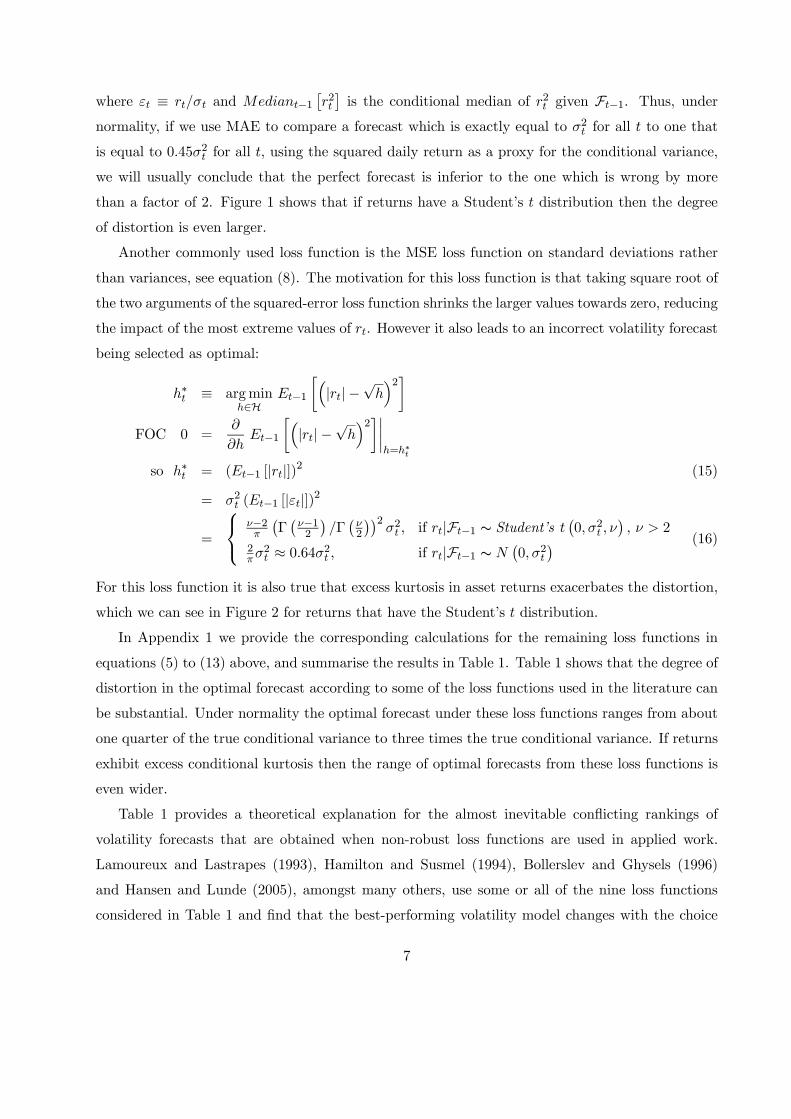
where εt ≡ rt/σt and Mediant−1£r2t¤is the conditional median of r2t given Ft−1. Thus, under
normality, if we use MAE to compare a forecast which is exactly equal to σ2t for all t to one that
is equal to 0.45σ2t for all t, using the squared daily return as a proxy for the conditional variance,
we will usually conclude that the perfect forecast is inferior to the one which is wrong by more
than a factor of 2. Figure 1 shows that if returns have a Student’s t distribution then the degree
of distortion is even larger.
Another commonly used loss function is the MSE loss function on standard deviations rather
than variances, see equation (8). The motivation for this loss function is that taking square root of
the two arguments of the squared-error loss function shrinks the larger values towards zero, reducing
the impact of the most extreme values of rt. However it also leads to an incorrect volatility forecast
being selected as optimal:
h∗t ≡ argminh∈H
Et−1
∙³|rt|−
√h´2¸
FOC 0 =∂
∂hEt−1
∙³|rt|−
√h´2¸¯
h=h∗t
so h∗t = (Et−1 [|rt|])2 (15)
= σ2t (Et−1 [|εt|])2
=
⎧⎨⎩ ν−2π
¡Γ¡ν−12
¢/Γ¡ν2
¢¢2σ2t , if rt|Ft−1 ∼ Student’s t
¡0, σ2t , ν
¢, ν > 2
2πσ
2t ≈ 0.64σ2t , if rt|Ft−1 ∼ N
¡0, σ2t
¢ (16)
For this loss function it is also true that excess kurtosis in asset returns exacerbates the distortion,
which we can see in Figure 2 for returns that have the Student’s t distribution.
In Appendix 1 we provide the corresponding calculations for the remaining loss functions in
equations (5) to (13) above, and summarise the results in Table 1. Table 1 shows that the degree of
distortion in the optimal forecast according to some of the loss functions used in the literature can
be substantial. Under normality the optimal forecast under these loss functions ranges from about
one quarter of the true conditional variance to three times the true conditional variance. If returns
exhibit excess conditional kurtosis then the range of optimal forecasts from these loss functions is
even wider.
Table 1 provides a theoretical explanation for the almost inevitable conflicting rankings of
volatility forecasts that are obtained when non-robust loss functions are used in applied work.
Lamoureux and Lastrapes (1993), Hamilton and Susmel (1994), Bollerslev and Ghysels (1996)
and Hansen and Lunde (2005), amongst many others, use some or all of the nine loss functions
considered in Table 1 and find that the best-performing volatility model changes with the choice
7

of loss function. Given that, for example, the MSE-prop loss function leads to an optimal forecast
that is biased upwards by at least a factor of three, while the MAE loss function leads to an optimal
forecast that is biased downwards by at least a factor of two, it is no surprise that different rankings
of volatility forecasts are found.
To illustrate and emphasize the empirical relevance of the results of Table 1, consider the
following example.
Example 1: Assume that rt|Ft−1 ∼ N¡0, σ2t
¢, and that σ2t follows a simple GARCH(1,1)
process: σ2t = ω + βσ2t−1 + αr2t−1, subject to ω > 0 and 1− β2 − 2αβ − 3α2 > 0 (which is requiredfor E
£σ4t¤to exist). Let σ2t = r2t , let L be the MSE-SD loss function, and let h1t = σ2t and
h2t = 2/πσ2t . Let n denote the number of observations available for conducting the test. Then the
DMW test statistic evaluated at population moments is:
DMW0 =
Ã5 + 3
p2/π
1−p2/π
· 1− (α+ β)2
1− (α+ β)2 − 2α2− 1!−1/2
·√n
≈ 0.1632√n, when α = 0.05 and β = 0.9.
The derivation is in Appendix 1. For the specific case that [α, β] = [0.05, 0.9], which is reasonable
for daily asset returns, the DMW0 statistic is greater than 1.96 for sample sizes larger than 145.
Thus with less than a year’s worth of daily data, we would expect to reject the true conditional
variance in favour of a volatility forecast equal to around 0.64 times the true conditional variance.
This example shows that choosing an inappropriate loss function for volatility forecast comparison
can have important empirical implications in realistic situations.
2.2 Using better volatility proxies
It has long been known that squared returns are a quite noisy proxy for the true conditional
variance. One alternative volatility proxy that has gained much attention recently is “realised
volatility”, see Andersen, et al. (2001a, 2003), and Barndorff-Nielsen and Shephard (2002, 2004).
Another commonly-used alternative to squared returns is the intra-daily range. It is well-known
that if the log stock price follows a Brownian motion then both of these estimators are unbiased
and more efficient than the squared return.
In this section we obtain the rate at which the distortion in the ranking of alternative forecasts
disappears when using realised volatility as the proxy, as the sampling frequency increases, for a
simple data generating process (DGP). These results can be viewed as complements to that of
Hansen and Lunde (2006), who showed that under certain conditions the degree of distortion in
8

ranking alternative forecasts is increasing in the variability of the proxy error.
Assume that there are m equally-spaced observations per trade day, and let ri,m,t denote the ith
intra-daily return on day t. In order to obtain analytical results for problems involving the range
as a volatility proxy we consider only a simple DGP: zero mean return, no jumps, and constant
conditional volatility within a trade day8. Chen and Patton (2006) present corresponding results
for a range of more realistic DGPs via simulation. Let
rt = d logPt = σtdWt (17)
στ = σt ∀τ ∈ (t− 1, t] (18)
ri,m,t ≡i/mZ
(i−1)/m
rτdτ = σt
i/mZ(i−1)/m
dWτ (19)
so {ri,m,t}mi=1 ∼ iidN
µ0,σ2tm
¶(20)
We place no constraints on how σ2t changes between trade days, though the assumption of constant
intra-daily volatility is clearly restrictive. The “realised volatility” or “realised variance” is defined
as:
RVt ≡mXi=1
r2i,m,t
Realised variance, like the daily squared return (which is obtained in the above framework by
setting m = 1), is a conditionally unbiased estimator of the daily conditional variance. Its main
advantage is that it is more efficient estimator than the daily squared return: for this DGP it can
be shown that MSEt−1£r2t¤= 2σ4t while MSEt−1 [RVt] = 2σ4t /m.
A volatility proxy that pre-dates realised volatility by many years is the range, or the high/low,
estimator, see Parkinson (1980), Garman and Klass (1980) and Ball and Torous (1984). Alizadeh,
et al. (2002) use the fact that the range is widely available and is more efficient than squared returns
to improve the estimation of stochastic volatility models. The intra-daily log range is defined as:
RGt ≡ maxτlogPτ −min
τlogPτ , t− 1 < τ ≤ t (21)
Under the dynamics in equation (17) Feller (1951) presented the density of RGt, and Parkinson
(1980) presented a formula for obtaining moments of the range, which enable us to compute:
Et−1£RG2t
¤= 4 log (2) · σ2t ≈ 2.7726σ2t (22)
8Analytical and empirical results on the range and “realised range” under more flexible DGPs are presented in
two recent working papers by Christensen and Podolskij (2005) and Martens and van Dijk (2005).
9

Details on the distributional properties of the range under this DGP are presented in Appendix
1. The above expression shows that squared range is not a conditionally unbiased estimator of σ2t .
Most authors, see Parkinson (1980) and Alizadeh, et al. (2002) for example, who employ the range
as a volatility proxy are aware of this and scale the range accordingly. We will thus focus below on
the adjusted range:
RG∗t ≡RGt
2plog (2)
≈ 0.6006RGt (23)
which, when squared, is an unbiased proxy for the conditional variance. Using the results of
Parkinson (1980) it is simple to determine thatMSEt−1£RG∗2t
¤≈ 0.4073σ4t , which is approximately
one-fifth of the MSE of the daily squared return, and so using the range yields an estimator as
accurate as a realised volatility estimator constructed using 5 intra-daily observations. This roughly
corresponds to the comment of Andersen and Bollerslev (1998, footnote 20) that the adjusted range
yields an MSE comparable to the MSE of realised volatilities constructed using 2 to 3 hour returns.
We now determine the optimal forecasts obtained using the various loss functions considered
above, when σ2t = RVt or σ2t = RG∗2t is used as a proxy for the conditional variance rather than r2t .
We initially leave m unspecified for the realised volatility proxy, and then specialise to three cases:
m = 1, 13 and 78, corresponding to the use of daily, half-hourly and 5-minute returns, on a stock
listed on the New York Stock Exchange (NYSE).
For MSE and QLIKE the optimal forecast is simply the conditional mean of σ2t , which equals
the conditional variance, as RVt and RG∗2t are both conditionally unbiased. The MSE-SD loss
function yields (Et−1 [σt])2 as an optimal forecast. Under the set-up introduced above,
RVt ≡mXi=1
r2t,i =σ2tm
mXi=1
ε2t,i
so mσ−2t RVt ∼ χ2m
so h∗t =σ2tm
³Ehp
χ2m
i´2Ehp
χ2m
i≈√m− 1
4√mby a Taylor series approximation
so h∗t ≈ σ2t
µ1− 1
2m+
1
16m2
¶
≈
⎧⎪⎪⎨⎪⎪⎩0.5625 · σ2t for m = 1
0.9619 · σ2t for m = 13
0.9936 · σ2t for m = 78
The results for the MSE-SD loss function using realised volatility show that reducing the noise
10

in the volatility proxy improves the optimal forecast, consistent with Hansen and Lunde (2006).9
Using the range we find that
h∗t = (Et−1 [RG∗t ])2 =
2
π log 2σ2t ≈ 0.9184σ2t
and so the distortion from using the range is approximately equal to that incurred when using a
realised volatility constructed using 6 intra-daily observations.
Consider now the MAE loss function, which yields Mediant−1£σ2t¤as the optimal forecast. For
realised volatility we thus have
h∗t =1
mMedian
£χ2m¤σ2t
For largem,Median£χ2m¤≈ m−2/3, though most software packages have functions for the inverse
cdf of a χ2m distribution. For smallm the approximation Median£χ2m¤≈ m − 2/3 + 1/ (9m) is
more accurate. Thus
h∗t ≈µ1− 2
3m+
1
9m2
¶σ2t
≈
⎧⎪⎪⎨⎪⎪⎩0.4444 · σ2t for m = 1
0.9494 · σ2t for m = 13
0.9915 · σ2t for m = 78
using Median£χ2m¤≈ m− 2/3 + 1/ (9m)
For the range we have
h∗t ≈2.2938
log 16σ2t = 0.8273σ
2t
which is equivalent to using about 4 observations to construct the realised volatility proxy. Calcu-
lations for the remaining loss functions are collected in Appendix 1, and the results are summarised
in Table 2.
The results in Table 2 confirm that as the proxy used to measure the true conditional variance
gets more efficient the degree of distortion decreases for all loss functions. Across loss functions
we found that the range was generally approximately as good a volatility proxy as the realised
volatility estimator constructed with between 4 and 6 intra-daily observations. Using half-hour
returns (13 intra-daily observations) or the intra-daily range still leaves substantial distortions in
the optimal forecasts, but using 5-minute returns (78 intra-daily observations) eliminates almost
all of the bias, at least in this simple framework10.9Note that the result for m = 1 is different to that obtained in Section 2, which was h∗t =
2πσ
2t ≈ 0.6366σ2t . This
is because for m = 1 we can obtain the expression exactly, using results for the normal distribution, whereas for
arbitrary m we relied on a second-order Taylor series approximation.10Chen and Patton (2006) find very similar results to those in Table 2 when the DGP is specified to be log-normal,
11

2.3 General comments on non-robust loss functions
The sources of the mis-matches between the optimal forecast for a given loss function and the
true conditional variance are easily identified. The MAE, MAE-SD and MAE-prop loss functions
consider mean absolute distances rather than mean squared distances, which then naturally change
the solution of the optimisation problem from an expectation to a median. For the MSE-log, MSE-
SD and MSE-prop loss functions the distortion follows from the fact that the unbiasedness property
is not invariant to nonlinear transformations.
In all of these cases the distortions can be remedied if one can obtain a conditionally unbiased
estimator of the quantity of interest (σt, log σ2t , etc.) either exactly or approximately. When using
the squared return as a proxy, this will generally require an assumption about the entire conditional
distribution of returns. When using realised variance as a volatility proxy one may obtain an
approximate distribution of the volatility proxy under relatively mild assumptions, by drawing on
the distribution theory for realised volatility developed in Barndorff-Nielsen and Shephard (2004)
and extensions, as in Andersen, et al. (2005a). On the other hand, when using a robust loss
function only the assumption of conditional unbiasedness of the proxy is required, which is often
satisfied under much weaker assumptions and requires no adjustment of the proxy.
We now seek to identify the reason why some non-robust loss function yield upward-biased
forecasts, whilst others yield downward-biased forecasts. We do so by generalising the results
from the previous sections to a broad class of arbitrary loss functions, making use of Taylor series
approximations. This requires some differentiability assumptions on the loss function, which are
not satisfied for some of the loss functions considered above.
Assumption T1: The volatility proxy satisfies: Et−1£σ2t,m
¤= σ2t and Vt−1
£σ2t,m
¤= ν2t,m
Assumption T2: The loss function L is three times differentiable.
Assumption T3: The loss function L is such that L¡σ2, h
¢= 0 iff h = σ2
Assumption T4: The loss function L is such that ∂L¡σ2, h
¢∂h T 0 if σ2 S h
Assumption T5: The volatility proxy and the loss function are such that L¡σ2t,m, h
¢−
L¡σ2t , h
¢→p 0 as m→∞ uniformly on H.
Proposition 1 Define
h∗t,m ≡ argminh∈H
Et−1£L¡σ2t,m, h
¢¤GARCH or two-factor stochastic volatility diffusions. Using the same parameterisations as those in the simulations of
Goncalves and Meddahi (2005), they find slightly larger biases from the non-robust loss functions under these DGPs,
but they generally differ from those in Table 2 only in the second decimal place.
12

(i) Let assumptions T1-T4 hold. Then
∂3L¡σ2, h
¢∂ (σ2)2 ∂h
T 0 for all¡σ2, h
¢⇒ h∗t,m S σ2t
(ii) Let assumptions T3-T5 hold. Then h∗t,m →p σ2t as m→∞.
The first part of the above proposition shows that it is the sign of the third derivative of the
loss function that determines whether the optimal forecast is above, below or equal to the true
conditional variance. The case that this third derivative is equal to zero, and thus that the optimal
forecast is the conditional variance, corresponds to a result of Hansen and Lunde (2006). The third
derivative is always positive for the MSE-log and MSE-SD loss functions, and so part (i) above
implies that h∗t,m < σ2t for these loss functions, which is consistent with the results in Tables 1 and
2. Alternatively, for the MSE-prop loss function this third derivative is always negative, implying
that h∗t,m > σ2t for this loss function, which is again consistent with Tables 1 and 2.
The second part of the above proposition shows that under the high-level assumption of uniform
convergence of L¡σ2t,m, h
¢to L
¡σ2t , h
¢, the optimal forecast converges to the conditional variance
as m→∞. Thus even loss functions that cause distortions in the presence of noise in the volatilityproxy can generate optimal forecasts that are consistent for the conditional variance, and so non-
robust loss functions may be used in conjunction with proxies that can be assumed “nearly” perfect.
3 A class of robust loss functions
In the previous section we showed that amongst nine loss functions commonly used to compare
volatility forecasts, only the MSE and the QLIKE loss functions lead to h∗t = Et−1£σ2t¤= σ2t ,
which is a necessary condition for a loss function to be robust to noise in the volatility proxy. The
following proposition provides a necessary and sufficient class of robust loss functions, which are
related to the class of linear-exponential densities of Gourieroux, et al. (1984), and to the work of
Gourieroux, et al. (1987). We make the following assumptions:
A1: Et−1£σ2t¤= σ2t
A2: σ2t |Ft−1 ∼ Ft ∈ F , the set of all absolutely continuous distribution functions on R+.
A3: L is twice continuously differentiable with respect to h and σ2, and has a unique minimum
at σ2 = h.
A4: There exists some h∗t ∈ int (H) such that h∗t = Et−1£σ2t¤, where H is a compact subset of
R++.
13

A5: L and Ft are such that: (a) Et−1£L¡σ2t , h
¢¤<∞ for some h ∈ H; (b)
¯Et−1
£∂L¡σ2t , σ
2t
¢/∂h
¤¯<∞; and (c)
¯Et−1
£∂2L
¡σ2t , σ
2t
¢/∂h2
¤¯<∞ for all t.
Proposition 2 Let assumptions A1 to A5 hold. Then a loss function L is robust, in the sense of
Definition 1, if and only if it takes the following form:
L¡σ2, h
¢= C (h) +B
¡σ2¢+ C (h)
¡σ2 − h
¢(24)
where B and C are twice continuously differentiable, C is a strictly decreasing function on H, andC is the anti-derivative of C.
Remark 1 If we normalise the loss function to yield zero loss when σ2 = h, then the class of
robust loss functions takes the form:
L¡σ2, h
¢= C (h)− C
¡σ2¢+ C (h)
¡σ2 − h
¢(25)
where C is a twice continuously differentiable, strictly decreasing function on H, and C is the
anti-derivative of C.
Given the widespread interest in economics and finance in loss functions that depend only on
the forecast error or the standardised forecast error, we present below a surprising result on the
subset of robust loss functions that satisfy one of these restrictions.
Proposition 3 (i) The “MSE” loss function is the only robust loss function that depends solely
on the forecast error, σ2 − h.
(ii) The “QLIKE” loss function is the only robust loss function that depends solely on the
standardised forecast error, σ2/h.
The general representation of robust loss functions in Proposition 2 provides a simple means
of determining whether a given loss function is suitable for use in volatility forecast comparison,
but it does not directly provide new alternative robust loss functions. To this end, we now seek to
find a parametric family of loss functions, that is a member of the class proposed above, and which
nests MSE and QLIKE as special cases. We do this by noting that the first-order conditions from
MSE and QLIKE loss functions are both of the form:
∂L¡σ2, h
¢∂h
= 0 = ahb¡σ2 − h
¢, a < 0, b ∈ R (26)
From this first-order condition we obtain the following parametric family of robust loss functions.
Part (ii) below shows that this parametric family coincides with the subset of homogeneous robust
loss functions.
14

Proposition 4 (i) The following family of functions
L¡σ2, h; b
¢=
⎧⎪⎪⎨⎪⎪⎩1
(b+1)(b+2)(σ2b+4 − hb+2)− 1
b+1hb+1
¡σ2 − h
¢, for b /∈ {−1,−2}
h− σ2 + σ2 log σ2
h , for b = −1σ2
h − logσ2
h − 1, for b = −2
(27)
satisfy L (h, h; b) = 0 for all h ∈ H, and are of the form in Proposition 2.
(ii) The family of loss functions in part (i) corresponds to the entire subset of homogeneous
robust loss functions. The degree of homogeneity is equal to b+ 2.
The MSE loss function is obtained when b = 0 and the QLIKE loss function is obtained when
b = −2, up to additive and multiplicative constants. In Figure 3 we present the above class offunctions for various values of b, ranging from 1 to −5, and including the MSE and QLIKE cases.This figure shows that this family of loss functions can take a wide variety of shapes, ranging from
symmetric (b = 0, corresponding to the MSE loss function) to asymmetric, with heavier penalty
either on under-prediction (b < 0) or over-prediction (b > 0). Figure 4 plots the ratio of losses
incurred for negative forecast errors to those incurred for positive forecast errors, to make clearer
the form of asymmetries in these loss functions.
Given the arbitrariness of the choice of units in most economic and financial problems (for
example, measuring prices in dollars versus cents, or measuring returns in percentages versus deci-
mals) it is potentially interesting to consider the impact of a simple change in units on the ranking
of two competing forecasts by expected loss. The class of loss functions presented in Proposition
2 guarantees that the true conditional variance will be chosen (subject to sampling variation) over
any other forecast regardless of the choice units. However it does not guarantee that the ranking of
two imperfect forecasts will be invariant to the choice of units. The following proposition shows that
by using a homogeneous robust loss function, as in Proposition 4, the ranking of any two (possibly
imperfect) forecasts is invariant to a re-scaling of the data. It further provides an example where
the ranking can be reversed simply with a re-scaling of the data if a non-homogeneous robust loss
function is used.
Proposition 5 (i) The ranking of any two (possibly imperfect) volatility forecasts by expected loss
is invariant to a re-scaling of the data if the loss function is robust and homogeneous.
(ii) The ranking of any two (possibly imperfect) volatility forecasts by expected loss may not be
invariant to a re-scaling of the data if the loss function is robust but not homogeneous.
Having presented a new class of loss functions, it is next of interest to establish the conditions
under which we can employ these loss functions in DMW tests for volatility forecast comparison.
15

The main conditions to be determined are moment conditions on the volatility proxy and volatility
forecasts, and these are presented in part (ii) of the following proposition.
Proposition 6 Let dt (b) ≡ L¡σ2t , h1t; b
¢− L
¡σ2t , h2t; b
¢. (i) For a given loss function parameter
b, and given that
1. (a) dt (b) = d0 (b) + εt (b), t = 1, 2, ...; d0 (b) ∈ R,
(b) {dt (b)} is a mixing sequence with either φ of size −r/2 (r − 1) for some r ≥ 2, or α ofsize −r/ (r − 2) for some r > 2,
(c) E [dt (b)] = d0 (b) for t = 1, 2, ...,
(d) E [|dt (b)|r] < ∆ <∞ for all t, and
(e) Vn (b) ≡ V£n−1/2
Pnt=1 εt (b)
¤is uniformly positive definite.
Then √n¡d (b)− d0 (b)
¢pVn (b)
→D N (0, 1) , as n→∞
where dn (b) ≡ n−1Pn
t=1 dt (b). Under H0 : E [dt (b)] = 0, we have:
DMWn (b) ≡√ndn (b)q
V£√
ndn (b)¤ →D N (0, 1) as n→∞
where V£√
ndn (b)¤is any consistent estimator of V
£√ndn (b)
¤. If E [dt (b)] 6= 0 then DMWn (b)→
±∞.(ii) Sufficient conditions for E
hdt (b)
2i<∞ are
1. inft hit ≡ ci > 0 for i = 1, 2,
2. E [hpit] <∞, i = 1, 2, and
3. E [σqt ] <∞,
where p and q are as follows:
p = max [0, 2b+ 4] , q = max [4 + δ, 4b+ 8] , for δ > 0, when b /∈ {−1,−2}p = 2 (e+ 1) /e ≈ 2.74, q = 4 (e+ 1) /e ≈ 5.47, when b = −1p = 2/e+ δ ≈ 0.74 + δ, q = 4 + δ, for δ > 0, when b = −2
where e is the exponential constant, e ≈ 2.71.
16

The assumption that the volatility forecasts will never be less than some positive threshold is
true for many standard volatility models, such as the GARCH(1,1), for example. Part (ii) of the
above proposition show how greatly the moment conditions can vary depending on the choice of
loss function shape parameter b. For MSE loss, corresponding to b = 0, we need E£h4it¤and E
£σ8t¤
to be finite, whereas for the QLIKE loss function we only require Ehh2/e+δit
iand E
hσ4+δt
i, for
δ > 0, to be finite. Choosing b ≤ −2 is recommended if the existence of moments of the volatilityproxy or volatility forecasts is a concern.
4 Empirical application to forecasting IBM return volatility
In this section we consider the problem of forecasting the conditional variance of the daily return
on IBM, using data from the TAQ database over the period from January 1993 to December 2003.
We consider two simple volatility models that are widely-used in industry: a 60-day rolling window
estimator, and the RiskMetrics volatility model based on daily returns:
Rolling window : h1t =1
60
X60
j=1r2t−j (28)
RiskMetrics : h2t = λh2t−1 + (1− λ) r2t−1, λ = 0.94 (29)
We use approximately the first year of observations (272 observations) to initiate the RiskMetrics
forecasts, and the remaining 2500 observations to compare the forecasts. A plot of the volatility
forecasts is provided in Figure 5.
We employ a variety of volatility proxies in the comparison of these forecasts: the daily squared
return, and realised variance computed using 65-minute, 15-minute and 5-minute returns11. In
comparing these forecasts we present the results of Diebold-Mariano-West tests using the loss
function presented in Proposition 4, for five different choices of the loss function parameter: b =
{1, 0,−1,−2,−5}. MSE loss and QLIKE loss correspond to b = 0 and b = −2 respectively. Recallfrom the previous section that different choices of b require weaker or stronger moment conditions
for the DMW test to be valid. For b = −5 we only require Ehσ4+δt
i< ∞ for δ > 0, whereas for
b = 1 we need E£h6it¤< ∞ and E
£σ12t¤< ∞. These assumptions should be kept in mind when
interpreting the results below.
Table 3 presents the results of standard Mincer-Zarnowitz tests of the volatility forecasts. Both
the rolling window and the RiskMetrics forecasts are rejected using all four volatility proxies, with
11We use 65-minute returns rather than 60-minute returns so that there are an even number of intervals within the
NYSE trade day, which runs from 9.30am to 4pm.
17
MZ test p-values equal to 0.00 in all cases. We can thus conclude that neither of these forecasts is
optimal. This conclusion leads then to the question of relative forecast performance, for which we
use a DMW test.
In Table 4 we present tests comparing the RiskMetrics forecasts based on daily returns with
the 60-day rolling window volatility forecasts. The only loss function for which the difference in
forecast performance is significantly different from zero is the QLIKE loss function: the difference
is significant at the 0.05 level using 65-minute, 15-minute and 5-minute realised variances as the
volatility proxy, and significant at the 0.10 level using daily squared returns as the proxy. In all
of these cases the t-statistic is positive, indicating that the rolling window forecasts generated
larger average loss than the RiskMetrics forecasts. Interestingly, under MSE loss, the differences
in average loss favour the rolling window forecasts, though these differences are not statistically
significant.
5 Conclusion
We analytically demonstrated some problems with volatility forecast comparison techniques used
in the literature. These techniques invariably rely on a volatility proxy, which is some imperfect
estimator of the true conditional variance, and the presence of noise in the volatility proxy can lead
an imperfect volatility forecast being selected over the true conditional variance for certain choices
of loss function. We showed analytically that less noisy volatility proxies, such as the intra-daily
range and realised volatility, lead to less distortion, though in some cases the degree of distortion
is still large.
We derived necessary and sufficient conditions on the loss function for it to yield rankings of
volatility forecasts that are robust to noise in the proxy. We also proposed a new parametric
family of robust loss functions and derived the moment conditions necessary for the use of this
loss function in forecast comparison tests. The new family of loss function nests both squared-
error and the “QLIKE” loss functions, two of the most widely-used in the volatility forecasting
literature. A small empirical study of IBM equity volatility illustrated the new loss functions in
forecast comparison tests.
Whilst volatility forecasting is a prominent example of a problem in economics where the variable
of interest is unobserved, there are many other such examples: forecasting the true rates of inflation
or GDP growth (not simply the announced rates); forecasting trade intensities; forecasting default
probabilities or ‘crash’ probabilities; and forecasting covariances or correlations. The derivations in
18

this paper exploited the fact that the latent variable of interest in volatility forecasting (namely the
conditional variance) is a positive random variable, and the proxy is non-negative and continuously
distributed. Extending the results in this paper to handle latent variables of interest with support
on the entire real line, as would be required for applications to studies of the “true” rates of growth
in macroeconomic aggregates or to conditional covariances, should not be difficult. Extending
our results to handle proxies with discrete support, such as those that would be used in default
forecasting applications, may require a different method of proof. We leave such extensions to
future research.
6 Appendix 1: Supporting calculations for Section 2
Section 2.1:
Optimal forecasts under alternative loss functions. Recall that εt ≡ rt/σt.
MSE-log:
h∗t = exp©Et−1
£log ε2t
¤ªσ2t
=
⎧⎨⎩ (ν − 2) exp©Ψ¡12
¢−Ψ
¡ν2
¢ªσ2t , if rt|Ft−1 ∼ Student’s t
¡0, σ2t , ν
¢, ν > 2
12 exp {−γE}σ2t ≈ 0.28σ2t , if rt|Ft−1 ∼ N
¡0, σ2t
¢where Ψ is the digamma function and γE = −Ψ (1) ≈ 0.58 is Euler’s constant, see Harvey, et al. (1994).
MSE-prop:
h∗t =Et−1
£r4t¤
Et−1£r2t¤ = Kurtosist−1 [rt]σ
2t
=
⎧⎨⎩ 3³ν−2ν−4
´σ2t , if rt|Ft−1 ∼ Student’s t
¡0, σ2t , ν
¢, ν > 4
3σ2t , if rt|Ft−1 ∼ N¡0, σ2t
¢QLIKE: h∗t = Et−1
£r2t¤= σ2t
MAE-log: h∗t = exp©Mediant−1
£log ε2t
¤ªσ2t =Mediant−1
£ε2t¤σ2t , since Median [log (X)] =
log (Median [X]) for any non-negative random variable X. Thus the optimal forecast is identical to that
under MAE loss, which is given in the body of the paper.
MAE-SD: h∗t = (Mediant−1 [|εt|])2 σ2t =Mediant−1£ε2t¤σ2t , sinceMedian [X]2 =Median
£X2¤
for any non-negative random variable X. Thus the optimal forecast is identical to that under MAE loss,
which is given in the body of the paper.
19

MAE-prop: If r2t |Ft−1 ∼ Ft¡σ2t¢and ε2t ≡ r2t /σ
2t |Ft−1 ∼ Gt (1) then
FOC 0 =
Z h∗t
0
r2th∗t
ft¡r2t¢dr2t −
Z ∞
h∗t
r2th∗t
ft¡r2t¢dr2t
soZ h∗t
0
r2th∗t
ft¡r2t¢dr2t =
Z ∞
h∗t
r2th∗t
ft¡r2t¢dr2t
Ft (h∗t )Et−1
∙r2th∗t
¯r2t ≤ h∗t
¸= (1− Ft (h
∗t ))Et−1
∙r2th∗t
¯r2t > h∗t
¸without loss of generality let h∗t ≡ σ2tγ
∗t , γ
∗t > 0, so
Ft¡σ2tγ
∗t
¢Et−1
∙ε2tγ∗t
¯ε2t ≤ γ∗t
¸=
¡1− Ft
¡σ2tγ
∗t
¢¢Et−1
∙ε2tγ∗t
¯ε2t > γ∗t
¸Gt (γ
∗t )Et−1
£ε2t¯ε2t ≤ γ∗t
¤= (1−Gt (γ
∗t ))Et−1
£ε2t¯ε2t > γ∗t
¤If ε2t |Ft−1 ∼ G (1), then γ∗t = γ∗ ∀ t. Finding an explicit expression for h∗t is difficult, and so we used
10,000 simulated draws for ν = {4, 6, 10, 20, 30, 50, 100, 1000,∞} and numerically obtained h∗t for each
ν. We then used OLS to find the approximation given in Table 1, which yielded an R2 of 0.9667.
DMW test using MSE-SD loss: We have
dt = (|rt|− σt)2 −
³|rt|−
p2/πσt
´2and we seek to find an expression for DMW0 as a function of (ω, α, β, n), where DMW0 ≡V£√
ndn¤−1/2√
nE [dt]. In the interests of parsimony we present results under the incorrect assump-
tion that dt is serially uncorrelated, which leads to the simplification DMW0 = V [dt]−1/2√nE [dt] . In
unreported work we also derived the variance allowing for serial correlation in dt and found that accounting
for the serial correlation does not change the conclusion significantly. The serial correlation in dt turns out
to be negative, and so the correct variance is slightly smaller than the naïve variance estimator used, which
makes the coefficient on√n even larger.
dt = (|rt|− σt)2 −
³|rt|−
p2/πσt
´2= (1− 2/π)σ2t + 2
³p2/π − 1
´|εt|σ2t
so E [dt] =³1−
p2/π
´2E£σ2t¤
and
E£d2t¤= E
∙σ4tEt−1
∙³1− 2/π + 2 |εt|
³p2/π − 1
´´2¸¸=
³1−
p2/π
´3 ³5 + 3
p2/π
´E£σ4t¤
20

The quantities E£σ2t¤and E
£σ4t¤depend on the DGP for the returns, and in this case they equal:
E£σ2t¤=
ω
1− α− β, if α+ β < 1
E£σ4t¤=
ω2 (1 + α+ β)³1− (α+ β)2 − 2α2
´(1− α− β)
, if³1− (α+ β)2 − 2α2
´> 0
so
DMW0 =
√n³1−
p2/π
´2E£σ2t¤r³
1−p2/π
´3 ³5 + 3
p2/π
´E£σ4t¤−³1−
p2/π
´4E£σ2t¤2
=
Ã5 + 3
p2/π
1−p2/π
1− (α+ β)2
1− (α+ β)2 − 2α2− 1!−1/2√
n
as stated in the text. Note that the parameter ω does not affect the statistic.
Section 2.2:
Wherever possible we derived solutions or approximate solutions analytically. This was not always
possible and so in some cases we had to resort to simulations to obtain solutions. Feller (1951) presents the
density of the range:
f (RGt;σt) = 8∞Xk=1
(−1)k−1 k2
σtφ
µk ·RGt
σt
¶where φ is the standard normal pdf . For practical purposes the sum in the above expression needs to be
truncated at some finite value; we truncate at k = 1000. Parkinson (1980) presented the cdf of the range,
and a formula for obtaining moments:
F (RGt;σt) =∞Xk=1
(−1)k−1 k½erfc
µ(k + 1)RGt
σ√2
¶− 2erfc
µk ·RGt
σ√2
¶+ erfc
µ(k − 1)RGt
σ√2
¶¾E [RGp
t ] =4√πΓ
µp+ 1
2
¶³2p/2 − 22−p/2
´ζ (p− 1)σpt , for p ≥ 1
where erfc(x) ≡ 1− erf(x), erf(x) is the ‘error function’: erf (x) ≡ 2/√πR∞0 e−t
2dt. ζ is the Riemann
zeta function. From this expression we can obtain the necessary moments for computing optimal forecasts
when the range is used as a volatility proxy. For the first and second moments of RGt we can obtain simple
expressions, but the fourth moment involves ζ (3) = Σ∞k=1k−3 which is an irrational number, and thus only
a numerical expression is available. In addition to the moments of RGt, we will need the mean of logRGt
and the median of RGt. We used quadrature and OLS to obtain the expression12:
Et−1 [logRGt] = 0.4257 + log σt (30)12We used quadrature to estimate Et−1 [logRGt] for σt = 0.5, 1, 1.5, ..., 10. We then regressed these esti-
mates on a constant and log σt to obtain the parameter estimates. The R2 from this regression was 1.0000.
21

which is consistent with the expression given in Alizadeh, et al. (2002). We numerically inverted the cdf of
the range, given in Parkinson (1980), and used OLS to determine the following relation13:
Mediant−1 [RGt] = 1.5145σt
so Mediant−1£RG2t
¤= 2.2938σ2t , since RGt is weakly positive.
MSE-LOG: h∗t = exp©Et−1
£log σ2t
¤ª. A Taylor series approximation did not provide a good fit
when considering realised variance as a proxy, and so we resorted to simulations. We simulated 50,000 “days”
worth of observations, where the number of observations per day considered was m =
{1, 3, 5, 7, 10, 13, 20, 40, 60, 78, 100}. The following expression yielded anR2 of 0.9959 : Et−1hlogRV
(m)t
i≈
−1.2741/m, so the optimal forecast under our DGP assumption is h∗t ≈ σ2t e−1.2741/m.
For the range we find that
Et−1£logRG∗2t
¤= 2Et−1 [logRG
∗t ]
= −0.1684 + log σ2tso h∗t = e−0.1684σ2t ≈ 0.8450σ2t
MAE-log: The optimal forecast is h∗t = Mediant−1£σ2t¤, since σ2t is weakly positive we know that
log¡Mediant−1
£σ2t¤¢= Mediant−1
£log σ2t
¤, and so the results for this loss function are identical to
those for the MAE loss function.
MAE-SD: The optimal forecast is h∗t =Mediant−1£σ2t¤. Since σ2t is weakly positive we know that
Mediant−1£σ2t¤= (Mediant−1 [σt])
2, and so the results for this loss function are identical to those for
the MAE loss function.
MSE-prop: h∗t = Et−1£σ4t¤/Et−1
£σ2t¤. When realised volatility is used as the proxy we find: h∗t =¡
1mKurtosist−1 [rt,i] +
m−1m
¢σ2t =
¡1 + 2
m
¢σ2t . For the range we find that: h
∗t = 10.8185/
³(log 16)2
´σ2t ≈
1.4073σ2t .
MAE-prop: For realised variance, like the daily squared return, obtaining an analytical, even approx-
imate, solution to this problem is difficult and so we used simulations. In the set-up given in the text it
is again possible to show that the optimal forecast is of the form h∗t = γ∗σ2t . For realised volatility we
simulated 50,000 “days” worth of observations, where the number of observations per day considered was
13The R2 from this relation for σ = 0.5, 1, 1.5, ..., 10 was 1.0000.
22
m = {1, 3, 5, 7, 10, 13, 20, 40, 60, 78, 100}, and used numerical methods to locate the optimum forecast.
The following expression yielded an R2 of 0.9999 : h∗t ≈¡1 + 1.3624
m
¢σ2t . For the range we again used a
numerical minimisation algorithm combined with quadrature to compute the expectation in the optimisation
problem: h∗t ≈ 0.9941σ2t .
7 Appendix 2: Proofs of Propositions
Proof of Proposition 1. (i) Approximate the loss function L with a second-order Taylor series:
L¡σ2t,m, h
¢≈ L
¡σ2t , h
¢+
∂L¡σ2t , h
¢∂σ2t
¡σ2t,m − σ2t
¢+1
2
∂2L¡σ2t , h
¢∂¡σ2t¢2 ¡
σ2t,m − σ2t¢2
so Et−1£L¡σ2t,m, h
¢¤≈ L
¡σ2t , h
¢+
1
2m
∂2L¡σ2t , h
¢∂¡σ2t¢2 ν2t,m
by assumption T1. The first-order condition for forecast optimality is
0 = Et−1
"∂L¡σ2t,m, h
∗t,m
¢∂h
#
≈∂L¡σ2t , h
∗t,m
¢∂h
+1
2m
∂3L¡σ2t , h
∗t,m
¢∂¡σ2t¢2∂h
ν2t,m
In the absence of noise in the volatility proxy (i.e. ν2t,m = 0) the second term above would equal zero
and the first-order condition would be the same as if the true conditional variance was observable.
By assumption T4 this yields h∗t,m = σ2t . One of the conditions of Hansen and Lunde (2006) was
∂3L¡σ2, h
¢/∂¡σ2¢2∂h = 0, which implies that the second term above equals zero even in the
presence of a noisy volatility proxy. For loss functions that yield ∂3L¡σ2, h
¢/∂¡σ2¢2∂h 6= 0 the
presence of noise in the volatility proxy distorts the first-order condition from what it would be in the
absence of noise, and thus affects the optimal forecast. If ∂3L¡σ2, h
¢/∂¡σ2¢2∂h > (<) 0 ∀
¡σ2, h
¢,
then the FOC implies that we must have ∂L¡σ2t , h
∗t,m
¢/∂h < (>) 0, which implies that h∗t,m <
(>) σ2t , by assumption T4.
(ii) Follows from Theorem 3.4 of White (1994), noting that assumptions T3 and T4 imply that
h∗ = σ2 is the unique solution to the problem minh∈H L¡σ2, h
¢.
Proof of Proposition 2. We prove this proposition by showing the equivalence of the
following three statements:
S1: The loss function takes the form given the statement of the proposition;
S2: The loss function is robust in the sense of Definition 1;
23

S3: The optimal forecast under the loss function is the conditional variance.We will show that S1⇒ S2, and then that S1⇔ S3, and finally that S2⇒ S3.That S1⇒ S2 follows from Hansen and Lunde (2006): their assumption 2 is satisfied given the
assumptions for the proposition and noting that ∂2L¡σ2, h
¢/∂¡σ2¢2= B00
¡σ2¢does not depend
on h.
We next show that S1⇒ S3: The first-order condition defining the optimal forecast is:
0 =∂
∂h
¡Et−1
£L¡σ2t , h
∗t
¢¤¢=
∂
∂h
³C (h∗t ) +Et−1
£B¡σ2t¢¤+ C (h∗t )
¡Et−1
£σ2t¤− h∗t
¢´= C 0 (h∗t )
¡Et−1
£σ2t¤− h∗t
¢which implies h∗t = Et−1
£σ2t¤since C is a strictly decreasing function. The second-order condition
is also satisfied: ∂2¡Et−1
£L¡σ2t , h
∗t
¢¤¢/∂h2 = C 00 (h∗t )
¡Et−1
£σ2t¤− h∗t
¢− C 0 (h∗t ) = −C0 (h∗t ) > 0,
since h∗t = Et−1£σ2t¤and C is strictly decreasing.
Proving S3 ⇒ S1 is more challenging. For this part we follow the proof of Theorem 1 of
Komunjer and Vuong (2004), adapted to our problem. We seek to show that the functional form of
the loss function given in the proposition is necessary for h∗t = Et−1£σ2t¤, for any Ft ∈ F . Notice
that we can write∂L¡σ2t , ht
¢∂h
= c¡σ2t , ht
¢ ¡σ2t − ht
¢where c
¡σ2t , ht
¢=¡σ2t − ht
¢−1∂L¡σ2t , ht
¢/∂h, since σ2t 6= ht a.s. by assumption A2. Now decom-
pose c¡σ2t , ht
¢into
c¡σ2t , ht
¢= Et−1
£c¡σ2t , ht
¢¤+ εt
where Et−1 [εt] = 0. Thus
Et−1
"∂L¡σ2t , h
∗t
¢∂h
#= Et−1
£c¡σ2t , h
∗t
¢ ¡σ2t − h∗t
¢¤= Et−1
£c¡σ2t , ht
¢¤Et−1
£σ2t − h∗t
¤+Et−1
£εt¡σ2t − h∗t
¢¤If Et−1
£∂L¡σ2t , h
∗t
¢/∂h
¤= 0 for h∗t = Et−1
£σ2t¤, then it must be that Et−1
£σ2t − h∗t
¤= 0 ⇒
Et−1£εt¡σ2t − h∗t
¢¤= 0 for all Ft ∈ F . Employing a generalised Farkas lemma, see Lemma 8.1 of
Gourieroux and Monfort (1996), this implies that ∃ λ ∈ R such that λ¡σ2t − h∗t
¢= εt
¡σ2t − h∗t
¢for
every Ft ∈ F and for all t. Since σ2t − h∗t 6= 0 a.s. by assumption A2 this implies that εt = λ a.s.
for all t. Since Et−1 [εt] = 0 we then have λ = 0. Thus c¡σ2t , h
∗t
¢= Et−1
£c¡σ2t , h
∗t
¢¤for all t, which
implies that c¡σ2t , h
∗t
¢= c (h∗t ), and thus that ∂L
¡σ2t , ht
¢/∂h = c (ht)
¡σ2t − ht
¢.
24

A necessary condition for h∗t to minimise Et−1£L¡σ2t , h
¢¤is that Et−1
£∂2L
¡σ2t , h
∗t
¢/∂h2
¤≥ 0,
using A5 to interchange expectation and differentiation. Using the previous result we have:
Et−1
"∂2L
¡σ2t , h
∗t
¢∂h2
#= Et−1
£c0 (h∗t )
¡σ2t − h∗t
¢− c (h∗t )
¤= −c (h∗t )
which is non-negative iff c (h∗t ) is non-positive. From assumption A4 we know that the optimum is
in the interior of H and so we know that c 6= 0, and thus c (h) < 0 ∀ h ∈ H. To obtain the lossfunction corresponding to the given first derivative we simply integrate up:
L¡σ2, h
¢= σ2
Zc (h) dh−
Zc (h)hdh
= B¡σ2¢+ σ2C (h)−C (h)h+
ZC (h) dh
= C (h) +B¡σ2¢+ C (h)
¡σ2 − h
¢where C is a strictly decreasing function (i.e. C 0 ≡ c is negative) and C is the anti-derivative of C.
By assumption A3 both B and C are twice continuously differentiable. Thus S3⇒ S1.Finally, we show that S2⇒ S3: by the definition of h∗t we have
Et−1£L¡σ2t , h
∗t
¢¤≤ Et−1
hL³σ2t , ht
´ifor any other ht ∈ Ft−1
so E£L¡σ2t , h
∗t
¢¤≤ E
hL³σ2t , ht
´iby the LIE
and E£L¡σ2t , h
∗t
¢¤≤ E
hL³σ2t , ht
´isince L is robust under S2
But L¡σ2, h
¢has a unique minimum at σ2 = h, and if we set ht = σ2t ∈ Ft−1 then it must be the
case that h∗t = σ2t . This completes the proof.
Proof of Proposition 3. Without loss of generality, we work below with loss functions
that have been normalised to imply zero loss when the forecast error is zero: L¡σ2, h
¢= C (h) −
C¡σ2¢+C (h)
¡σ2 − h
¢.
(i) We want to find the general sub-set of loss functions that satisfy L¡σ2, h
¢= L
¡σ2 − h
¢∀¡σ2, h
¢for some function L. This condition implies
∂L¡σ2, h
¢∂σ2
= −∂L¡σ2, h
¢∂h
∀¡σ2, h
¢−C
¡σ2¢+ C (h) +C 0 (h)
¡σ2 − h
¢= 0 ∀
¡σ2, h
¢Taking the derivative of both sides w.r.t. σ2 we obtain:
−C 0¡σ2¢+ C 0 (h) = 0 ∀
¡σ2, h
¢which implies C 0 (h) = κ1 ∀ h
25

and since we know C is strictly decreasing, we also have κ1 < 0.
so C (h) = κ1h+ κ2¡σ2¢
C (h) =1
2κ1h
2 + κ2¡σ2¢h+ κ3
¡σ2¢
where κ2, κ3 are constants of integration, and may be functions of σ2. Thus the loss function
becomes
L¡σ2, h
¢=
1
2κ1h
2 + κ2¡σ2¢h+ κ3
¡σ2¢
−12κ1σ
4 − κ2¡σ2¢σ2 − κ3
¡σ2¢
+¡κ1h+ κ2
¡σ2¢¢ ¡
σ2 − h¢
= −12κ1¡σ2 − h
¢2Since proportionality constants do not affect the loss function, we find that the only loss function
that depends on¡σ2, h
¢only through the forecast error, σ2 − h, is the MSE loss function.
(ii) We next want to find the general sub-set of loss functions that satisfy L¡σ2, h
¢= L
¡σ2/h
¢∀¡σ2, h
¢for some function L. Note that this condition implies that L is homogeneous of degree zero. Using
Proposition 4 below, this implies that the loss function must be of the form:
L¡σ2, h
¢=
σ2
h− log σ
2
h− 1
which is the QLIKE loss function up to additive and multiplicative constants.
Proof of Proposition 4. (i) It is obvious L (h, h; b) = 0 ∀ h ∈ H. We now show that allthree of these loss functions are of the form in Proposition 2.
b /∈ {−1,−2}: C (h) = − (b+ 1)−1 hb+1, C (h) = − (b+ 1)−1 (b+ 2)−1 hb+2, B¡σ2¢=
(b+ 1)−1 (b+ 2)−1 σ2b+4.
b = −1: C (h) = − log h, C (h) = h− h logh, B¡σ2¢= σ2 log σ2 − σ2.
b = −2: C (h) = h−1, C (h) = log h, B¡σ2¢= − log σ2.
(ii) We seek the subset of robust loss functions that are homogeneous of order k : L¡aσ2, ah
¢=
akL¡σ2, h
¢∀ a > 0. Let
λ¡σ2, h
¢≡ ∂L
¡σ2, h
¢/∂h
= C 0 (h)¡σ2 − h
¢for robust loss functions.
Since L is homogeneous of order k, λ is homogeneous of order (k − 1) . This implies λ¡aσ2, ah
¢=
ak−1λ¡σ2, h
¢= ak−1C 0 (h)
¡σ2 − h
¢, while direct substitution yields λ
¡aσ2, ah
¢= aC 0 (ah)
¡σ2 − h
¢.
Thus C 0 (ah) = ak−2C 0 (h) ∀ a > 0, that is, C 0 is homogeneous of order (k − 2) .
26

Next we apply Euler’s theorem to C 0: C 00 (h)h = (k − 2)C 0 (h) ∀h > 0 , and so
(2− k)C 0 (h) + C 00 (h)h = 0
We can solve this first-order differential equation to find:
C 0 (h) = γhk−2
where γ is an unknown scalar. Since C 0 < 0 we know that γ < 0, and as this is just a scaling
parameter we set it to −1 without loss of generality.
C 0 (h) = −hk−2
C (h) =
⎧⎨⎩ 11−kh
k−1 + z1 k 6= 1− log h+ z1 k = 1
C (h) =
⎧⎪⎪⎨⎪⎪⎩z1h+
1k(1−k)h
k + z2 k /∈ {0, 1}z1h+ h− h logh+ z2 k = 1
z1h+ logh+ z2 k = 0
where z1 and z2 are constants of integration. Finally, we substitute the expressions for C and C
into equation (25) and simplify to obtain the loss functions in equation (27) with k = b+ 2.
Proof of Proposition 5. (i) If L is homogeneous then L¡aσ2, ah
¢= akL
¡σ2, h
¢∀a > 0
for some k. Then E£L¡aσ2t , ah1t
¢¤≥ E
£L¡aσ2t , ah2t
¢¤⇔ E
£akL
¡σ2t , h1t
¢¤≥ E
£akL
¡σ2t , h2t
¢¤⇔
E£L¡σ2t , h1t
¢¤≥ E
£L¡σ2t , h2t
¢¤, for any a > 0.
(ii) Here we need only provide an example. Consider the following stylised case: σ2t = 1 ∀t,(h1t, h2t) = (γ1, γ2) ∀t, and σ2t is such that Et−1
£σ2t¤= 1 a.s. ∀t. As a robust but non-homogeneous
loss we will use the one generated by the following specification for C 0:
C 0 (h) = − log (1 + h)
so C (h) = h− (1 + h) log (1 + h)
and C (h) =1
4
hh (3h+ 2)− 2 (1 + h)2 log (1 + h)
iFor small h this loss function resembles the the b = 1 loss function from Proposition 4 (up to
a scaling constant), but for medium to large h this loss function does not correspond to any in
Proposition 4.
27

Given this set-up, we have
E£L¡aσ2t , ahit
¢¤=
1
4
haγi (3aγi + 2)− 2 (1 + aγi)
2 log (1 + aγi)i−E
hC¡aσ2t
¢i+a [aγi − (1 + aγi) log (1 + aγi)] (1− γi)
Then define
dt (γ1, γ2, a) ≡ L¡aσ2t , aγ1
¢− L
¡aσ2t , aγ2
¢E [dt (γ1, γ2, a)] =
a
4(γ1 − γ2) (2− 4a− a (γ1 + γ2))
+1
2
³a2 (γ1 − 1)2 − (1 + a)2
´log (1 + aγ1)
−12
³a2 (γ2 − 1)2 − (1 + a)2
´log (1 + aγ2)
Then note that E [dt (1/3, 3/2, 1)] = −0.0087, and so the first forecast has lower expected loss thanthe second using the “original” scaling of the data. But E [dt (1/3, 3/2, 2)] = 0.0061, and so if all
variables are multiplied by 2 then the second forecast has lower expected loss than the first.
Proof of Proposition 6. (i) Follows directly from Exercise 5.21 of White (1999).
(ii) For b /∈ {−1,−2} we have:
dt (b) =1
b+ 2
³hb+21t − hb+22t
´− 1
b+ 1σ2t
³hb+11t − hb+12t
´so dt (b)
2 =1
(b+ 2)2
³h2b+41t + h2b+42t − 2hb+21t hb+22t
´+
1
(b+ 1)2σ4t
³h2b+21t + h2b+22t − 2hb+11t hb+12t
´− 2
(b+ 1) (b+ 2)σ2t
³h2b+31t + h2b+32t − hb+21t hb+12t − hb+11t hb+22t
´The largest terms in this expression are: (a) h2b+4it , (b) σ4th
2b+2it and (c) σ2th
2b+3it for i = 1, 2 . The
expectation of first term is finite by assumption. (b) If b > −1, then by Hölder’s inequality:
Ehσ4th
2b+2it
i≤ E
h¡σ4t¢b+2i1/(b+2)
E
∙³h2b+2it
´(b+2)/(b+1)¸(b+1)/(b+2)= E
hσ4b+8t
i1/(b+2)Ehh2b+4it
i(b+1)/(b+2)< ∞ by assumption.
If b < −1, then we will make use of the assumption that inft hit ≡ ci > 0 for i = 1, 2. This
assumption implies that h−1it is bounded below by zero and above by c−1i , and thus all moments of
28

h−1it exist.
Ehσ4th
2b+2it
i≤ E
h¡σ4t¢(4+δ)/4i4/(4+δ)
E
∙³h2b+2it
´(4+δ)/δ¸δ/(4+δ), for δ > 0
= Ehσ4+δt
i4/(4+δ)Ehh2(b+1)(4+δ)/δit
iδ/(4+δ)which is finite as E
hσ4+δt
i< ∞ by assumption, and E
hh−Mit
i< ∞ for all 0 ≤ M < ∞ since h−1it
is a bounded random variable. (c) If b > −1.5, then
Ehσ2th
2b+3it
i≤ E
hσ4b+8t
i1/(2b+4)E
∙³h2b+3it
´(2b+4)/(2b+3)¸(2b+3)/(2b+4)= E
hσ4b+8t
i1/(2b+4)Ehh2b+4it
i(2b+3)/(2b+4)< ∞ by assumption.
If b < −1.5,
Ehσ2th
2b+3it
i≤ E
h¡σ2t¢(4+δ)/2i2/(4+δ)
E
∙³h2b+3it
´(4+δ)/(2+δ)¸(2+δ)/(4+δ)= E
hσ4+δt
i2/(4+δ)Ehh(2b+3)(4+δ)/(2+δ)it
i(2+δ)/(4+δ)which is finite as E
hσ4+δt
i< ∞ by assumption, and E
hh−Mit
i< ∞ for all 0 ≤ M < ∞ since h−1it
is a bounded random variable.
Now consider b = −1. Here we have
dt = h1t − h2t − σ2t logh1th2t
so d2t = (h1t − h2t)2 + σ4t (log (h1t)− log (h2t))2
−2σ2t (log (h1t)− log (h2t)) (h1t − h2t)
The largest terms in this expression are: (a) h2it, (b) σ4t (log hit)
2 and (c) σ2thit log hit. The first
term is finite by assumption. For (b) we have
Ehσ4t (log hit)
2i≤ E
h¡σ4t¢(e+1)/eie/(e+1)
Eh(log hit)
2(e+1)i1/(e+1)
= Ehσ4(e+1)/et
ie/(e+1)Eh(log hit)
2(e+1)i1/(e+1)
29

The first term on the right-hand side is finite by assumption. For the second term note:
(log h)k ≤ hk/e ∀ h ≥ 1 for k > 0
And Eh(log hit)
ki≡
Z ∞
ci
(log hit)k fit (hit) dhit
=
Z 1
ci
(log hit)k fit (hit) dhit +
Z ∞
1(loghit)
k fit (hit) dhit¯Z 1
ci
(log hit)k fit (hit) dhit
¯< ∞ for k > 0 since ci > 0
Z ∞
1(loghit)
k fit (hit) dhit ≤Z ∞
1hk/eit fit (hit) dhit
≤Z ∞
ci
hk/eit fit (hit) dhit
≡ Ehhk/eit
iSo E
h(log hit)
2(e+1)i<∞ if E
hh2(e+1)/eit
i<∞, which holds by assumption. For (c) we have
E£σ2thit loghit
¤≤ E
h¡σ2t¢(2e+1)/eie/(2e+1)
Ehh(2e+1)/eit
ie/(2e+1)Eh(log hit)
2e+1i1/(2e+1)
< ∞
As the first two terms on the right-hand side are finite by assumption, and the final term is finite
given that the second term is finite and ci > 0.
Finally consider b = −2. We have
dt = σ2t
µ1
h1t− 1
h2t
¶+ log
h1th2t
so d2t = σ4t
µ1
h1t− 1
h2t
¶2+ 2 (logh1t − logh2t)2
+2σ2t
µ1
h1t− 1
h2t
¶log h1t − 2σ2t
µ1
h1t− 1
h2t
¶log h2t
with largest terms: (a) σ4th−2it , (b) (log hit)
2, (c) σ2th−1it log hit, and (d) σ
2th−1jt log hit for i = 1, 2 and
j 6= i. For term (a) we have
E
∙σ4t1
h2it
¸≤ E
h¡σ4t¢(4+δ)/4i4/(4+δ)
E
"µ1
h2it
¶(4+δ)/δ#δ/(4+δ), for δ > 0
= Ehσ4+δt
i4/(4+δ)Ehh−2(4+δ)/δit
iδ/(4+δ)The first term on the right-hand side is finite by assumption and the second term is finite since
ci > 0. For term (b) recall from above that if ci > 0 then Eh(log hit)
ki< ∞ if E
hhk/eit
i< ∞ for
30

k > 0. So Eh(log hit)
2i< ∞ is finite if E
hh2/eit
i< ∞, which holds by assumption. For term (c)
we use
E£σ2th
−1it log hit
¤≤ E
h¡σ2t¢(4+δ)/2i2/(4+δ)
Eh¡h−1it log hit
¢(4+δ)/(2+δ)i(2+δ)/(4+δ)for δ > 0
= Ehσ4+δt
i2/(4+δ)Eh¡h−1it log hit
¢(4+δ)/(2+δ)i(2+δ)/(4+δ)which is finite as the first term is finite by assumption and the second term is finite since h−1it log hit
is a bounded random variable if ci > 0. For the term in (d) we have
Ehσ2th
−1jt log hit
i≤ E
h¡σ2t loghit
¢(1+δ/4)i1/(1+δ/4)Ehh−(4+δ)/δjt
iδ/(4+δ), for δ > 0
≤ÃE
∙³σ2(1+δ/4)t
´2¸1/2E
∙³(log hit)
(1+δ/4)´2¸1/2!1/(1+δ/4)
Ehh−(4+δ)/δjt
iδ/(4+δ)=
µEhσ4+δt
i1/2Eh(log hit)
2+δ/2i1/2¶1/(1+δ/4)
Ehh−(4+δ)/δjt
iδ/(4+δ)The first term is finite by assumption, and the third term is finite as ci > 0. The second term
is finite if Ehh(2+δ/2)/eit
iis finite, and E
hh(2+δ/2)/eit
i< E
hh2/e+δit
i, which is finite by assumption.
This completes the proof.
31

8 Tables and Figures
Table 1: Optimal forecasts under various loss functions
Optimal forecast, h∗t
Loss function rt|Ft−1 ∼ Student0s t¡0, σ2t , ν
¢rt|Ft−1 ∼ Ft
¡0, σ2t
¢ν ν = 6 ν = 10 ν →∞
MSE σ2t σ2t σ2t σ2t σ2t
QLIKE σ2t σ2t σ2t σ2t σ2t
MSE-LOG exp©Et−1
£log ε2t
¤ªσ2t exp
©Ψ¡12
¢−Ψ
¡ν2
¢ª(ν − 2)σ2t 0.22σ2t 0.25σ2t 0.28σ2t
MSE-SD (Et−1 [|εt|])2 σ2t ν−2π
¡Γ¡ν−12
¢/Γ¡ν2
¢¢2σ2t 0.56σ2t 0.60σ2t 0.64σ2t
MSE-prop Kurtosist−1 [rt]σ2t 3ν−2ν−4σ2t 6.00σ2t 4.00σ2t 3.00σ2t
MAE Mediant−1£r2t¤
ν−2ν Median [F1,ν ]σ
2t 0.34σ2t 0.39σ2t 0.45σ2t
MAE-LOG Mediant−1£r2t¤
ν−2ν Median [F1,ν ]σ
2t 0.34σ2t 0.39σ2t 0.45σ2t
MAE-SD Mediant−1£r2t¤
ν−2ν Median [F1,ν ]σ
2t 0.34σ2t 0.39σ2t 0.45σ2t
MAE-prop† n/a¡2.36 + 1.00
ν + 7.78ν2
¢σ2t 2.73σ2t 2.55σ2t 2.36σ2t
Notes: This table presents the forecast that minimises the conditional expected loss when the squared
return is used as a volatility proxy. That is, h∗t minimises Et−1£L¡r2t , h
¢¤, for various loss functions L.
The first column presents the solutions when returns have an arbitrary conditional distribution Ft with
mean zero and conditional variance σ2t , the second, third, and fourth columns present results with returns
have the standardised Student’s t distribution, and the final column presents the solutions when returns
are conditionally normally distributed. Γ is the gamma function and Ψ is the digamma function. †The
expressions given for MAE-prop are based on a numerical approximation, see Appendix 1 for details.
32

Table 2: Optimal forecasts under various loss functions, using realised volatility and range
Volatility proxy
Loss function Realised volatility
Range Arbitrary m m = 1 m = 13 m = 78 m→∞MSE σ2t σ2t σ2t σ2t σ2t σ2t
QLIKE σ2t σ2t σ2t σ2t σ2t σ2t
MSE-LOG† 0.85σ2t e−1.2741/mσ2t 0.28σ2t 0.91σ2t 0.98σ2t σ2t
MSE-SD 0.92σ2t1m
³Ehp
χ2m
i´2σ2t 0.56σ2t 0.96σ2t 0.99σ2t σ2t
MSE-prop 1.41σ2t¡1 + 2
m
¢σ2t 3.00σ2t 1.15σ2t 1.03σ2t σ2t
MAE 0.83σ2t1mMedian
£χ2m¤σ2t 0.45σ2t 0.95σ2t 0.99σ2t σ2t
MAE-LOG 0.83σ2t1mMedian
£χ2m¤σ2t 0.45σ2t 0.95σ2t 0.99σ2t σ2t
MAE-SD 0.83σ2t1mMedian
£χ2m¤σ2t 0.45σ2t 0.95σ2t 0.99σ2t σ2t
MAE-prop† 1.19σ2t¡1 + 1.3624
m
¢σ2t 2.36σ2t 1.10σ2t 1.02σ2t σ2t
Notes: This table presents the forecast that minimises the conditional expected loss when the range or
realised volatility is used as a volatility proxy. That is, h∗t minimises Et−1£L¡σ2t , h
¢¤, for σ2t = RG∗2t or
σ2t = RVt, for various loss functions L. In all cases returns are assumed to be generated as a zero mean
Brownian motion with constant volatility within each trade day and no jumps. The cases ofm = 1, 13, 78
correspond to the use of daily squared returns, realised variance with 30-minute returns and realised variance
with 5-minute returns respectively. The case that m → ∞ corresponds to the case where the conditional
variance is observable ex-post without error. †For the MSE-LOG and MAE-prop loss functions we used
simulations, numerical integration and numerical optimisation to obtain the expressions given. Details on
the computation of the figures in this table are given in Appendix 1.
33
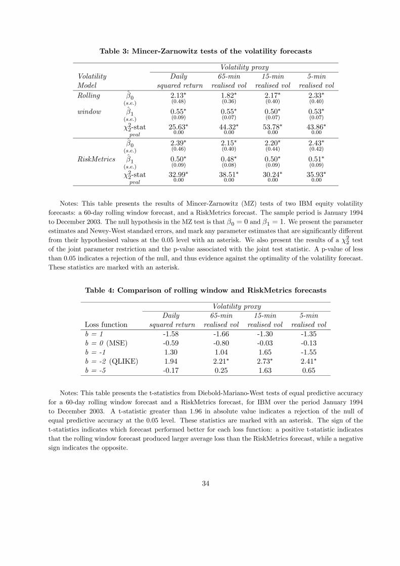
Table 3: Mincer-Zarnowitz tests of the volatility forecasts
Volatility proxyVolatility Daily 65-min 15-min 5-minModel squared return realised vol realised vol realised volRolling β0
(s.e.)
2.13∗(0.48)
1.82∗(0.36)
2.17∗(0.40)
2.33∗(0.40)
window β1(s.e.)
0.55∗(0.09)
0.55∗(0.07)
0.50∗(0.07)
0.53∗(0.07)
χ22-statpval
25.63∗0.00
44.32∗0.00
53.78∗0.00
43.86∗0.00
β0(s.e.)
2.39∗(0.46)
2.15∗(0.40)
2.20∗(0.44)
2.43∗(0.42)
RiskMetrics β1(s.e.)
0.50∗(0.09)
0.48∗(0.08)
0.50∗(0.09)
0.51∗(0.09)
χ22-statpval
32.99∗0.00
38.51∗0.00
30.24∗0.00
35.93∗0.00
Notes: This table presents the results of Mincer-Zarnowitz (MZ) tests of two IBM equity volatilityforecasts: a 60-day rolling window forecast, and a RiskMetrics forecast. The sample period is January 1994to December 2003. The null hypothesis in the MZ test is that β0 = 0 and β1 = 1. We present the parameterestimates and Newey-West standard errors, and mark any parameter estimates that are significantly differentfrom their hypothesised values at the 0.05 level with an asterisk. We also present the results of a χ22 testof the joint parameter restriction and the p-value associated with the joint test statistic. A p-value of lessthan 0.05 indicates a rejection of the null, and thus evidence against the optimality of the volatility forecast.These statistics are marked with an asterisk.
Table 4: Comparison of rolling window and RiskMetrics forecasts
Volatility proxyDaily 65-min 15-min 5-min
Loss function squared return realised vol realised vol realised volb = 1 -1.58 -1.66 -1.30 -1.35b = 0 (MSE) -0.59 -0.80 -0.03 -0.13b = -1 1.30 1.04 1.65 -1.55b = -2 (QLIKE) 1.94 2.21∗ 2.73∗ 2.41∗
b = -5 -0.17 0.25 1.63 0.65
Notes: This table presents the t-statistics from Diebold-Mariano-West tests of equal predictive accuracyfor a 60-day rolling window forecast and a RiskMetrics forecast, for IBM over the period January 1994to December 2003. A t-statistic greater than 1.96 in absolute value indicates a rejection of the null ofequal predictive accuracy at the 0.05 level. These statistics are marked with an asterisk. The sign of thet-statistics indicates which forecast performed better for each loss function: a positive t-statistic indicatesthat the rolling window forecast produced larger average loss than the RiskMetrics forecast, while a negativesign indicates the opposite.
34

References
[1] Alizadeh, Sassan, Brandt, Michael W., and Diebold, Francis X., 2002, Range-Based Estimationof Stochastic Volatility Models, Journal of Finance, 57(3), 1047-1091.
[2] Andersen, Torben G., Benzoni, Luca, and Lund, Jesper, 2002, An Empirical Investigation ofContinuous-Time Equity Return Models, Journal of Finance, 57(3), 1239-1284.
[3] Andersen, Torben G., and Bollerslev, Tim, 1998, Answering the Skeptics: Yes, StandardVolatility Models Do Provide Accurate Forecasts, International Economic Review, 39, 885-905.
[4] Andersen, Torben G., Bollerslev, Tim, and Lange, Steve, 1999, Forecasting Financial MarketVolatility: Sample Frequency Vis-à-vis Forecast Horizon, Journal of Empirical Finance, 6,457-477.
[5] Andersen, Torben, Bollerslev, Tim, and Diebold, Francis X., 2002, “Parametric and Non-parametric Volatility Measurement,” forthcoming in L.P. Hansen and Y. Ait-Sahalia (eds.),Handbook of Financial Econometrics, Amsterdam: North-Holland.
[6] Andersen, Torben, Bollerslev, Tim, Diebold, Francis X., and Ebens, Heiko, 2001a, The Distri-bution of Realized Stock Return Volatility, Journal of Financial Economics, 61, 43-76.
[7] Andersen, Torben G., Bollerslev, Tim, Diebold, Francis X. and Labys, Paul, 2001b, The Distri-bution of Realized Exchange Rate Volatility, Journal of the American Statistical Association,96, 42-55.
[8] Andersen, Torben G., Bollerslev, Tim, Diebold, Francis X. and Labys, Paul, 2003, Modelingand Forecasting Realized Volatility, Econometrica, 71(2), 579-625.
[9] Andersen, Torben G., Bollerslev, Tim, and Meddahi, Nour, 2004, Analytic Evaluation ofVolatility Forecasts, International Economic Review, 45, 1079-1110.
[10] Andersen, Torben G., Bollerslev, Tim, and Meddahi, Nour, 2005a, Correcting the Errors:Volatility Forecast Evaluation Using High-Frequency Data and Realized Volatilities, Econo-metrica, 73(1), 279-296.
[11] Andersen, Torben G., Bollerslev, Tim, Christoffersen, Peter F., and Diebold, Francis X., 2005b,Volatility and Correlation Forecasting, in the Handbook of Economic Forecasting, G. Elliott,C.W.J. Granger and A. Timmermann ed.s, North Holland Press, Amsterdam.
[12] Ball, Clifford A., and Torous, Walter N., 1984, The Maximum Likelihood Estimation of Secu-rity Price Volatility: Theory, Evidence, and Application to Option Pricing, Journal of Business,57(1), 97-112.
[13] Barndorff-Nielsen, Ole E., and Shephard, Neil, 2002, Econometric Analysis of Realised Volatil-ity and Its Use in Estimating Stochastic Volatility Models, Journal of the Royal StatisticalSociety, Series B, 64, 253-280.
[14] Barndorff-Nielsen, Ole E., and Shephard, Neil, 2004, Econometric Analysis of Realized Covari-ation: High Frequency Based Covariance, Regression and Correlation in Financial Economics,Econometrica, 72(3), 885-925.
35

[15] Bollerslev, Tim, and Ghysels, Eric, 1994, Periodic Autoregressive Conditional Heteroscedas-ticity, Journal of Business and Economic Statistics, 14(2), 139-151.
[16] Bollerslev, Tim, and Wright, Jonathan H., 2001, High-Frequency Data, Frequency DomainInference, and Volatility Forecasting, Review of Economics and Statistics, 83(5), 596-602.
[17] Chen, Runquan and Patton, Andrew J., 2006, Volatility Forecast Evaluation and Comparison,work-in-progress, To be published in T.G. Andersen, R.A. Davis, J.-P. Kreiss and T. Mikosch(eds.) Handbook of Financial Time Series, Springer Verlag.
[18] Christensen, Kim, and Podolskij, Mark, 2005, Asymptotic Theory for Range-Based Estimationof Integrated Variance of a Continuous Semi-Martingale, working paper, Aarhus School ofBusiness.
[19] Christoffersen, Peter and Diebold, Francis X., 1997, Optimal prediction under asymmetricloss, Econometric Theory, 13, 808-817.
[20] Christoffersen, Peter, and Jacobs, Kris, 2004, The Importance of the Loss Function in OptionValuation, Journal of Financial Economics, 72, 291-318.
[21] Clements, Michael P., 2005, Evaluating Econometric Forecasts of Economic and FinancialVariables, Palgrave MacMillan, United Kingdom.
[22] Cowles, Alfred, 1933, Can Stock Market Forecasters Forecast?, Econometrica, 1(3), 309-324.
[23] Diebold, Francis X., and Mariano, Roberto S., 1995, Comparing Predictive Accuracy, Journalof Business and Economic Statistics, 13(3), 253-263.
[24] Diebold, Francis X., and Lopez, Jose A., 1996, Forecast Evaluation and Combination, in G.S.Maddala and C.R. Rao (eds.), Handbook of Statistics, Amsterdam: North-Holland, 241-268.
[25] Engle, Robert F., 1982, Autoregressive Conditional Heteroskedasticity With Estimates of theVariance of U.K. Inflation, Econometrica, 50, 987-1008.
[26] Engle, Robert F., 1993, A Comment on Hendry and Clements on the Limitations of ComparingMean Square Forecast Errors, Journal of Forecasting, 12, 642-644.
[27] Engle, R.F., C.-H. Hong, A. Kane and J. Noh, 1993, Arbitrage valuation of variance forecastswith simulated options, in: D. Chance and R. Tripp, eds., Advances in Futures and OptionsResearch, JIA Press, Greenwich, U.S.A.
[28] Feller, W., 1951, The Asymptotic Distribution of the Range of Sums of Random Variables,Annals of Mathematical Statistics, 22, 427-432.
[29] Garman, Mark B., and Klass, Michael J., 1980, On the Estimation of Security Price Volatilitiesfrom Historical Data, Journal of Business, 53(1), 67-78.
[30] Gonçalves, Sílvia, and Meddahi, Nour, 2005, Bootstrapping Realized Volatility, working paper,Université de Montréal.
[31] Gourieroux, C., Monfort, A., and Trognon, A., 1984, Pseudo Maximum Likelihood Methods:Theory, Econometrica, 52(3), 681-700.
36

[32] Gourieroux, C., Monfort, A. and Renault, E., 1987, Consistent M-Estimators in a Semi-Parametric Model, CEPREMAP working paper 8720.
[33] Gourieroux, C. and Monfort, A., 1996, Statistics and Econometric Models, Volume 1, trans-lated from the French by Q. Vuong, Cambridge University Press, Great Britain.
[34] Granger, C.W.J., 1969, Prediction with a generalized cost function, OR, 20, 199-207.
[35] Hamilton, James D., and Susmel, Rauli, 1994, Autoregressive Conditional Heteroskedasticityand Changes in Regime, Journal of Econometrics, 64(1-2), 307-333.
[36] Hansen, Peter Reinhard, and Lunde, Asger, 2005, A Forecast Comparison of Volatility Models:Does Anything Beat a GARCH(1,1)?, Journal of Applied Econometrics, 20(7), 873-889.
[37] Hansen, Peter R., and Lunde, Asger, 2006, Consistent Ranking of Volatility Models, Journalof Econometrics, 131(1-2), 97-121.
[38] Harvey, Andrew, Ruiz, Esther, and Shephard, Neil, 1994, Multivariate Stochastic VolatilityModels, Review of Economic Studies, 61, 247-264.
[39] Huber, P.J., 1981, Robust Statistics, Wiley, New York, U.S.A.
[40] Komunjer, I., and Vuong, Q., 2004, Efficient Conditional Quantile Estimation, working paper.
[41] Lamoureux, C.G. and Lastrapes, W.D., 1993, Forecasting Stock Return Variance: Toward anUnderstanding of Stochastic Implied Volatilities, Review of Financial Studies, 6(2), 293-326.
[42] Martens, Martin, and van Dijk, Dick, 2005, Measuring Volatility with the Realized Range,Journal of Econometrics, forthcoming.
[43] Meddahi, Nour, 2001, A Theoretical Comparison between Integrated and Realized Volatilities,manuscript, Université de Montréal.
[44] Mincer, Jacob, and Zarnowitz, Victor, 1969, The Evaluation of Economic Forecasts, inZarnowitz, J. (ed.) Economic Forecasts and Expectations, National Bureau of Economic Re-search, New York.
[45] Newey, Whitney K., and West, Kenneth D., 1987, A Simple, Positive Semidefinite, Het-eroskedasticity and Autocorrelation Consistent Covariance Matrix, Econometrica, 55(3), 703-708.
[46] Pagan, Adrian R., and Schwert, G. William, 1990, Alternative Models for Conditional Volatil-ity, Journal of Econometrics, 45, 267-290.
[47] Parkinson, Michael, 1980, The Extreme Value Method for Estimating the Variance of the Rateof Return, Journal of Business, 53(1), 61-65.
[48] Patton, Andrew J., and Timmermann, Allan, 2004, Properties of Optimal Forecasts underAsymmetric Loss and Nonlinearity, Centre for Economic Policy Research Discussion Paper4037.
37

[49] Poon, Ser-Huang and Granger, Clive W. J., 2003, Forecasting Volatility in Financial Markets,Journal of Economic Literature, 41, 478-539.
[50] Shephard, Neil, 2005, Stochastic Volatility: Selected Readings, Oxford University Press, UnitedKingdom.
[51] West, Kenneth D., 2005, Forecast Evaluation, in the Handbook of Economic Forecasting, G.Elliott, C.W.J. Granger and A. Timmermann ed.s, North Holland Press, Amsterdam.
[52] West, Kenneth D., Edison, Hali J., and Cho, Dongchul, 1993, A Utility-Based Comparison ofSome Models of Exchange Rate Volatility, Journal of International Economics, 35, 23-45.
[53] White, Halbert, 1994, Estimation, Inference and Specification Analysis, Econometric SocietyMonographs No. 22, Cambridge University Press, Cambridge, U.K.
[54] White, Halbert, 1999, Asymptotic Theory for Econometricians, Revised Edition, AcademicPress, San Diego.
3 6 9 12 15 18 21 24 27 300.26
0.28
0.3
0.32
0.34
0.36
0.38
0.4
0.42
0.44
0.46
Kurtosis
Med
ian[
e2 ]
Optimal forecasts under MAE loss
Figure 1: Optimal forecasts under MAE loss when true variance is 1, for various levels of kurtosis,using the standardised Student’s t distribution. The dashed line represents the optimal forecast asν → 4.
38

3 6 9 12 15 18 21 24 27 300.48
0.5
0.52
0.54
0.56
0.58
0.6
0.62
0.64
Kurtosis
E[|e
|]2
Optimal forecasts under MSE-SD loss
Figure 2: Optimal forecasts under MSE-SD loss when true variance is 1, for various levels ofkurtosis, using the standardised Student’s t distribution. The dashed line represents the optimalforecast as ν → 4.
0 0.5 1 1.5 2 2.5 3 3.5 40
0.5
1
1.5
2
2.5
hhat (r2=2)
loss
Various robust loss functions
b=1b=0.5b=0 (MSE)b=-0.5b=-1b=-2 (QLIKE)b=-5
Figure 3: Loss functions for various choices of b. True σ2=2 in this example, with the volatilityforecast ranging between 0 and 4. b=0 and b=-2 correspond to the MSE and QLIKE loss functionsrespectively.
39

0 0.5 1 1.5 20
0.5
1
1.5
2
2.5
forecast error (r2=2)
loss
Ratio of loss from negative forecast errors to positive forecast errors
b=1b=0.5b=0 (MSE)b=-0.5b=-1b=-2 (QLIKE)b=-5
Figure 4: Ratio of losses from negative forecast errors to positive forecast errors, for various choicesof b. True σ2=2 in this example, with the volatility forecast ranging between 0 and 4. b=0 andb=-2 correspond to the MSE and QLIKE loss functions respectively.
Jan94 Jan95 Jan96 Jan97 Jan98 Jan99 Jan00 Jan01 Jan02 Jan03 Dec030
5
10
15
20
25
30
35Conditional variance forecasts
Con
ditio
nal v
aria
nce
60-day rolling windowRiskMetrics
Figure 5: Conditional variance forecasts for IBM returns from 60-day rolling window and RiskMet-rics models, January 1994 to December 2003.
40


