
© GWEFR Cyf 2008
Water Hammer and the Method of Characteristics
Introduction
IEEE Standard 1207-2004 “IEEE Guide for the Application of Turbine Governing Systems for
Hydroelectric Generating Units” [1] advocates the use of computer simulation for stability
studies on hydroelectric plant at an early stage in the project life-cycle. Predicting the dynamic
performance of a planned installation allows design constraints to be revised before
construction begins and reduces the time required for governor tuning when the system is
being commissioned.
The basic simulation models for hydroelectric plant, suitable for analysis and design of control
systems, are described in a well-known IEEE paper written by a group of industry experts [2].
Section 4.4 of the paper describes how travelling-wave effects in the water passages can be
simulated by solving the one-dimensional ‘water hammer’ equations by means of the Method of
Characteristics. The paper compares simulation results obtained by this method with simpler
models. It does not, however, include a detailed description of the solution method itself.
A conceptual description of the ‘water hammer’ phenomenon and the derivation of the
mathematical model as a hyperbolic partial differential equation is to be found in many sources,
such as the book by Larock et al [3]. The solution for a typical water hammer problem turns out
to be a pressure wave travelling back and forth along the conduit. An early analytical solution of
the basic wave equation is due to d’Alembert and this provides a valuable conceptual
explanation of the phenomena involved.
Analytical solutions prove to be impossible for just about any case of practical interest so it is
necessary to use numerical methods instead. Essentially, the Method of Characteristics converts
the partial differential equation into a ordinary differential equations whose validity is
constrained to a set of characteristic curves, related to the velocity of the travelling wave.
Typically, the method of finite differences is then applied to discretise the equations (temporally
and spatially) so that computer numerical integration techniques can be applied.
Further background will not be included here; instead, we simply present a summary of the
mathematics as a convenient supplement to the IEEE paper.
The water hammer equations
These are:
2
10
2
0
dV p dz fg V
a
Vdt x dx D
V dp
x dt
(1)
where:
x is the axial distance along the streamline
z is the elevation at any point of the streamline

V is the mean flow velocity
p is the pressure
a is the wave speed
is the fluid density
f is the Darcy-Weisbach friction factor
D is the pipe diameter
g is the acceleration due to gravity.
These equations have only one spatial dimension (x). For liquid flowing in a pipe, the flow
velocity (V) is considered to be uniform across the pipe cross-section. It is related to the
volumetric flow (Q) in any section of the pipe by the cross-sectional area: Q = AV.
Noting that:
( , )dV x t V dx V V VV
dt x dt t x t
dp p dx p p pV
dt x dt t x t
(2)
allows (1) to be simplified by omitting the ‘convective acceleration’ terms, which are usually
negligible in comparison with other terms, to leave:
2
10
2
0
V p dz fg V V
t x dx D
V p
x ta
(3)
Further analysis will proceed based on (3).
Bernoulli Equation
The Bernoulli equation states that the total head is constant along a streamline:
2
2
p Vz K
g (4)
where:
pH z
is the ‘piezometric head’,
z is the ‘elevation head’, 2
2
V
g is the ‘velocity head’ and

pis the ‘pressure head’.
g is known as the ‘specific weight’ of the fluid.
The velocity head term corresponds to the convective acceleration term in (2) and in many
cases of flow in pipes is negligible compared with frictional terms.
Analytical solution
Analytical solutions of (3) are restricted to simple cases.
For pipe flow, it is common practice to express (3) in terms of piezometric head (H) instead of
the pressure (p). To do this, note that:
and
H zg g
x x
p H zg g
p
x
t t t
(5)
where the term z
t
is zero because the pipe elevation does not change with time and
z
x
is
alternatively expressed as sin(), where is the angle at which the pipe slopes.
Substituting (5) into (3) allows the pipe slope term to be eliminated:
2
02
0a g
V H fg V V
t x D
V H
x t
(6)
The dissipative term V V in (6) is nonlinear (the friction depends on the sign of the velocity).
This makes an analytical solution very difficult, even for simple boundary conditions. To
proceed, consider the frictionless case and take the partial derivative of (6) with respect to both
t and x:
2 2
2
2
2 2
2
0
0
V Hg
t xt
V g H
t x a t
(7)
and

2
2 2
2
2 2
2
0
0
V Hg
x t x
V Ha g
x tx
(8)
Subtracting (8) from (7) yields:
2 2
2 2
2 22
2
2
2
0
0
V Va
t x
H Ha
t x
(9)
which are classic one-dimensional wave equations. These linear hyperbolic partial differential
equations can be solved individually for piezometric head or flow velocity.
An analytical solution to (9) is due to d’Alembert.
( ) ( ) 1( , ) ( )
2 2
x at
x at
f x at f x atH x t g s ds
a
(10)
where:
H(x,0) is the initial pressure profile across the pipe
( ,0)
( )H x
g xt
is the initial rate of change of pressure
The d’Alembert solution is the sum of two waves travelling in the opposite direction at the
constant wave velocity ‘a’. A complete solution is obtained by specifying initial conditions (at
t = 0) and boundary conditions (at x = 0 and x = L), where the boundary conditions are either
‘free’ or ‘fixed’.
The d’Alembert solution is extremely valuable as a concept for visualising and understanding
water hammer. Its use in practice is limited to cases which have a single dominant conduit and
very low levels of friction.
Practical solutions are usually obtained numerically by means of a finite difference form of the
Method of Characteristics.
Numerical solution by the Method of Characteristics
The following procedure changes the two PDEs in (3) into a single ODE.
Introduce the Lagrange multiplier :
2 02
1V pa
t
dz f V pg V V
dx D x tx (11)

Gather terms:
2
20
V p dV z fpa
t xg V V
x t dx D (12)
Now
( , )dV x t V V dx
xdt t dtso, by comparison of coefficients, the first term in (12) can be
made equal to dV
dtby letting:
2dxa
dt (13)
Also
( , )dp x t p dx p
dt x dt tand the second term in (12) can be made equal to
dp
dtby letting:
dx
dt (14)
So to satisfy both (13) and (14) we need:
2 2 2 2. a a with the solution:
a (15)
where is always positive but the wave velocity can be positive or negative.
By constraining a , the first two terms in (12) become full differentials:
2
0dp dz fdV
dg V V
dt dx Dt (16)
The PDEs (3) have been reduced to the single ODE (16) which applies at points where
dx
adt
and points where dx
adt
.
Choosing = a:
2
0dp dz f
gdV
a a adt
V Vdt dx D
2
10
dp dz fg
dVV V
dt dx Ddt a (17)
which is known as the C+ equation.

Similarly, choosing = -a:
1
20
dp dz fg
dV
dt daV V
t dx D (18)
which is known as the C- equation.
Again, it is possible to use the piezometric head (H) instead of the pressure (p) by recalling that
( ) ( )H z g H zp
dH dz dx
g gdtdt dx
dp
dt (19)
Substituting in the C+ equation (17):
1
20
dV dz dxg g
dt a dx dt
dH dz fg V V
dt dx D
02
dV g dz dx
dt a dx
dH g dz fg V V
dt a dx Ddt
Now substitution of dx
adt
, and similarly dx
adt
for the C- equation, gives:
02
02
dV g dH fV V
dt a dt D
dV g dH fV V
dt a dt D
+
-
C
C
(20)
Equations (20) are the basis for the finite-difference solution of the water hammer problem.
' 1For C , ' '
'' 1For C , '' ''
dx x ca x at c t x k
dt a a a
dx x ca x at c t x k
dt a a a
These represent a set of straight-line relationships between t and x on which C+ and C- are valid
as shown in the diagram below.
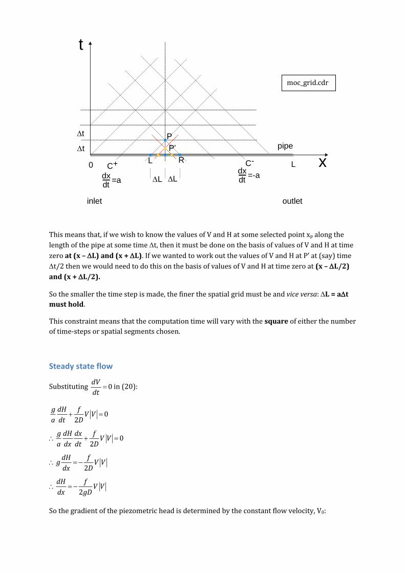
This means that, if we wish to know the values of V and H at some selected point xp along the
length of the pipe at some time t, then it must be done on the basis of values of V and H at time
zero at (x – L) and (x + L). If we wanted to work out the values of V and H at P’ at (say) time
t/2 then we would need to do this on the basis of values of V and H at time zero at (x – L/2)
and (x + L/2).
So the smaller the time step is made, the finer the spatial grid must be and vice versa: L = at
must hold.
This constraint means that the computation time will vary with the square of either the number
of time-steps or spatial segments chosen.
Steady state flow
Substituting 0dV
dt in (20):
02
02
2
2
g dH fV V
a dt D
g dH dx fV V
a dx dt D
dH fg V V
dx D
dH fV V
dx gD
So the gradient of the piezometric head is determined by the constant flow velocity, V0:
t
x
P
P’
RL
t
L L
t
0 LC+ C-
dxdt
=adxdt
=-a
pipe
inlet outlet
moc_grid.cdr

0 0( ) .2
i
fH x V V x c
gD
Let H(x=0) = Hres be the head at the reservoir. Then:
0 0(0) .02
res i
i res
fH H V V c
gD
c H
Let H(x=L) = HL be the head at the lower end of the pipe. Then:
0 0 0 0
0 0
( ) . .2 2
2( )
i res
res L
f fH L V V L c V V L H
gD gD
gDV V H H
fL
So the steady state velocity is given by:
0
2( )res L
gDV H H
fL (21)
Finite difference solution for the Method of Characteristics
The advantages of the finite-difference method are:
it is relatively easy to implement
it produces a numerical approximation to (20) on a rectangular grid in the xt plane
A disadvantage of the direct finite-difference method is that it generally does not directly
incorporate the fact that information about the solution of (20) is propagated along
characteristics. As a consequence, finite difference methods often produce poor results when
the solution has large gradients.
The major strength of the numerical method of characteristics is that it tracks information about
the solution along approximations to the characteristics. This makes the numerical method of
characteristics generally better at dealing with a solution that has sharp fronts. Its
disadvantages are:
it produces an approximation on an irregularly spaced set of points in the xt plane
it is somewhat more complicated to implement than a direct finite-difference method
Suppose we have N segments in a section of pipe, so that we have N+1 (spatial) sample points
separated by a distance L.

t
1 2 3 4 5 6 7
0 L
From (20), the C+ equation is:
02
dV g dH fV V
dt a dt D
A finite difference approximation for the velocity and head, (Vp, Hp), at point P in the diagram
above is expressed as:
provided
( )0
2
( )0
.
2
P P
P r P rr r
V V H Hg fV V
t a D
V V H Hg fV V
a t D
t
t
L a t
+C :
C : (22)
The subscripts ℓ and r in (22) refer to the sample points to the left and right of P and one time
interval t in the past. The relationship between L and t constrains the solution to the
characteristic lines*.
Multiplying through by t, equations (22) can be re-written:
( ) ( ) 02
( ) ( ) 02
P P
P r P r r r
g fV V H H V V
a D
g fV V H H V V
a
t
D
t
+C :
C :
(23)
Equation (23) may be solved for VP and HP. Let and 2
g fC K
a
t
D
0
1( ) ( )
2
P P
P r P r r r
P r r r r
V V CH CH KV V
V CH CH KV V V CH CH KV V
H V V C H H K V V V VC
In general, (VPi, HPi) at the ith sample point along the length of the pipe (where (i-1) and (i+1)
refer to the points to the left and right of P respectively) is given by:
* Computer code must build in this constraint when choosing sample time and segment length.
N=6 segments,
giving N+1 = 7
sample points

1 1 1 1 1 1 1 1
1 1 1 1 1 1 1 1
1
2 2
1
2 2
Pi i i i i i i i i
Pi i i i i i i i i
g fV V V H H V V V V
a D
a a fH V V H H V V V V
g g
t
D
t
(24)
Equations (24) are valid for interior points of the solution space, 2 i N .
Boundary conditions, valid for 0t , must be imposed on the two points at either end.
Initial conditions must be specified for t =0.
These are problem dependent. Many boundary conditions exist to describe the relationship
between flow and head for various pipe topologies such as constrictions and branches.
Boundary conditions
This section considers a small selection of common boundary conditions relevant to the solution
of hydraulic problems in the hydroelectric power generation industry.
Constant head reservoir at upstream end
Neglecting velocity head loss, the piezometric pressure at the inlet is fixed at the reservoir’s
elevation, Hin = Zres.
To get the boundary condition on flow velocity, use the C- relationship in (23) for the upstream
boundary:
1 1( ) 0P r P r r rV V C H H KV V
Now HP1 = Hin, Vr = V2 and Hr = H2 so:
1 2 2 2 2( )P inV V C H H KV V
Downstream valve
Assume that the valve is controlled to close such that the flow velocity decreases linearly over
the closure interval from an initial steady state value down to zero. Then the imposed boundary
condition is:
, 1 1 1P N ss ssc c
t j tV V V
t t
where j is the time-step index, tc is the valve closure interval and (N+1) refers to the rightmost
sample point on the pipe length.

Use the C+ relationship from (23) at the right-hand boundary:
( )
1( ) ( )
P P
P P
V V C H H KV V
KH H V V V V
C C
or, in terms of the boundary indices:
, 1 , 1
1P N N N P N N NH H V V KV V
C
Note that the value of the head is immediately available from the C+ expression because the
velocity is explicitly specified.
Change in pipe cross-sectional area
Suppose that there is a change in the cross-section of the pipe as shown here:
The pressure at P is identical for both sections if the loss at the constriction is considered
negligible. So the pressure at the right-most sample point (N+1) of the upstream section (i) is
identical to the left-most sample point (1) of the downstream section (i+1).†
, 1 1,1Pi N PiH H
Similarly, from continuity of flow:
, 1 1,1Pi N PiQ Q
The C- equation for the downstream section and the C+ equation for the upstream section are:
: ( ) 0
: ( ) 0
P P
P r P r r r
C V V C H H KV V
C V V C H H KV V
(25)
Applying these gives the following set of three equations to be solved for VP1,N+1, VP2,1, and
HP1,N+1 = HP2,1 = H0.
† Note that this convention means that point ‘N’ will be just to the left of ‘N+1’ in the upstream section and point ‘2’ will be just to the right of ‘1’ in the downstream section.
P V1 V2
D1, f1 D2, f2

1 1, 1 2 2,1
1, 1 1, 1, 1 1, 1 1, 1,
2,1 2,2 2,1 2,2 2 2,2 2,2
( ) 0
( ) 0
P N P
P N N P N N N N
P P
A V A V
V V C H H K V V
V V C H H K V V
(26)
where 1 21 2
1 2
and 2 2
f t f tK K
D D
are the friction terms for the two pipe sections.
Re-write (26):
1 1, 1 2 2,1
1, 1 1, 1 1, 1, 1 1, 1,
2,1 2,1 2,2 2,2 2 2,2 2,2
0
) 0
P N P
P N P N N N N N
P P
A V A V
V CH V CH K V V
V CH V CH K V V
(27)
and with the implied substitutions S1 and S2:
1 1, 1 2 2,1
1, 1 0 1
2,1 0 2
0
0
P N P
P N
P
A V A V
V CH S
V CH S
(28)
Solving (28) yields the required boundary conditions:
2 1 2 1 1 2 2 2 1 11, 1 2,1 0 1, 1 2,1
1 2 1 2 1 2
( ) ( ) 1 and and
( ) ( )P N P P N P
A S S A S S S A S AV V H H H
A A A A C A A
Note that a closed form solution of three linear simultaneous equations gives the unknown head
and velocities.
Pump/turbine
The following diagram represents a variable speed pump/turbine attached to both upstream
and downstream sections of pipe, of cross-sectional areas A1 and A2, diameters D1 and D2 and
friction factors f1 and f2, respectively.
The pump/turbine can be modelled at different levels of complexity. Let:
T = fT(Q, , G) is the shaft torque on the P/T
H1
P/T H2
datum
Hu
V1 V2
C+ C- A1, D1, f1 A2, D2, f2

Hu = H1 – H2 = fH(Q, , G) = change in head across the P/T as a function of flow (Q)
through the P/T, its rotational speed () and gate opening (G).
J = moment of inertia of P/T
dT J
dt
relates shaft torque to speed
The P/T characteristic is a static relationship but it is usual to assume that changes can be
represented as quasi-static, i.e. a simple migration of the P/T operating point. Clearly the
dynamics are more complex than this but a quasi-static model is more than adequate for this
level of system simulation. CFD modelling could be used for improved accuracy but the
complexity and computational burden are not warranted.
Knowing the values of V1, V2, H1, H2 and at time t, the goal is to calculate them at time t+t.
From continuity it is clear that V1A1 =V2A2. The problem lies in the fact that fT and fH are in
general nonlinear. When future values of HPi and VPi are calculated using equation (24), they
must lie on the turbine characteristic; in effect, the operating point has changed. In general it is
necessary to perform an iterative procedure to obtain consistent values of the variables at time
t+t.
A simpler case to consider is the boundary condition that exists when:
the P/T speed is assumed constant
one side of the P/T is connected to a constant head sump or tailrace
the gate opening is fixed
These restrict the head across the turbine to be a function of flow only: Hu = fH’(Q).
Suppose that the head across a turbine, whose inlet is downstream of a pipe of cross sectional
area A and whose outlet is connected to a constant pressure tailrace, is related to the flow
through the turbine by a quadratic equation:
2Hf ’ Q ' ' 'u t t tH A Q B Q C (29)
where A’t, B’t and C’t are constant parameters of the turbine.
If VP1 and HP1 are the velocity and head at point P at the turbine inlet at time (t+t) then:
1 1
1
2 21 1 1
21 1 1
' ' ( ' )
P P
u P tail
P t P t P t tail
P t P t P t
Q V A
H H H
H A A V B AV C H
H A V B V C
(30)
Hu
Q

The point of interest (P) at the turbine inlet is downstream of the last interior node of the
conduit which feeds it. So the required relationship is the (C+) characteristic equation in (23):
+, 1 , , 1 , , ,C : 0Pi N i N Pi N i N i N i N
gV V H H KV V
a (31)
In order to satisfy both (30) and (31) simultaneously:
2, 1 , , 1 , 1 , , ,
2, 1 , 1 , , , ,
0
(1 ) 0
Pi N i N t Pi N t Pi N t i N i N i N
t tPi N Pi N i N t i N i N i N
g gV V A V B V C H KV V
a a
gA gB g gV V V C H KV V
a a a a
(32)
where (32) is a quadratic equation that can be solved for VPi,N+1 and hence HPi,N+1 from (30).
By embedding the nonlinear turbine characteristic into the characteristic equations, we have
enforced solutions for flow velocity and head at the boundary at time t+t that are consistent
with both the turbine characteristic and the hydrodynamics. The turbine nonlinearity is simple
enough to lead to the quadratic equation (32) which can be solved by means of the usual
formula. More complex nonlinearities will usually need an iterative solution‡.
A variation that allows the gate opening (G) to be taken into account is to assume that both B’t
and C’t in (29) are zero (which reduces the turbine characteristic to the basic orifice equation).
Then: 2 2
' 'u t t
Q VH A A
GA G
(33)
where 0 < G < 1 is a linear modulation of the inlet area. (In practice this would be a nonlinear
relationship, dependent on the type of valve or gate vane in use).
The equation corresponding to (30) is now:
21
1 2P
P t tail
VH A H
G (34)
where At = A’t.
‡ This leads to a difficulty if the system is to be simulated in real-time because the time required to produce an iterative solution is unbounded.
Vi,N
Hi,N
P/T
datum
Hu
Vi,N+1
Hi,N+1
i+1
Vi+1,1
Hi+1,1
Vi+1,2
Hi+1,2
L
i

Now substituting (34) in (31) gives:
2, 1 , , 1 , , ,2
2, 1 , 1 , , , ,2
0
0
tPi N i N Pi N tail i N i N i N
tPi N Pi N i N i N tail i N i N
Ag gV V V H H KV V
a aG
gA g gV V V H H KV V
a aaG
(35)
At each time sample, equation (35) can be solved for VPi,N+1 and hence HPi,N+1 from (34). It is
important to note that this approach leads to difficulties as 0G because the quadratic
coefficient tends to infinity.
Pipe branch
The following diagram illustrates a pipe dividing into two branches.
In general, each branch will have a different friction coefficient and diameter (hence cross-
sectional area)
Continuity of flow requires that:
, 1 1 1,1 2 2,1i Pi N i Pi i PiAV A V A V (36)
Neglecting losses, the head at point P must be identical for all branches so:
, 1 1,1 2,1 0i N i iH H H H (37)
The characteristic equation for each branch must be satisfied:
, 1 , 0 0 , ,
1,1 1,2 0 0 1 1,2 1,2
2,1 2,2 0 0 2 2,2 2,2
( ) 0
( ) 0
( ) 0
Pi N i N P i i N i N
Pi i P i i i
Pi i P i i i
V V C H H K V V
V V C H H K V V
V V C H H K V V
(38)
P
Vi,N
Vi+2,2
Vi+1,2
Vi,N+1
Vi+1,1
Vi+2,1
C+
C-
C-
Ai, Di, fi
Ai+1, Di+1, fi+1
Ai+2, Di+2, fi+2

The goal is to find , 1 1,1 2,1 0, , and Pi N Pi Pi PV V V H by solving the simultaneous equations (36) and
(38). Letting:
, 0 , ,
1 1,2 0 1 1,2 1,2
2 2,2 0 2 2,2 2,2
i i N i i N i N
i i i i i
i i i i i
B V CH K V V
B V CH K V V
B V CH K V V
(39)
allows (36) and (38)to be expressed in the form L V B :
, 11 2
1,2
2,1 1
0 2
00
1 0 0
0 1 0
0 0 1
Pi Ni i i
Pi i
Pi i
P i
VA A A
V BC
V BC
H BC
(40)
which are solved as \V L B .
As for the case of change in cross-sectional area, a closed form solution of several linear
simultaneous equations yields the unknown head and velocities.
Conclusion
The expressions summarised in the preceding sections are implemented in Matlab/Simulink
and form the basis of the generic simulation package offered by GWEFR Cyf.
References
1 Std 1207-2004, 'IEEE Guide for the Application of Turbine Governing Systems for Hydroelectric Generating Units', New York, IEEE 2004.
2 IEEE Working group: 'Hydraulic turbine and turbine control models for system dynamic studies', IEEE Trans Power Systems, 1992, 7, (1), pp. 167-179.
3 Larock, B. E., Jeppson, R. W. and Watters, G. Z.: 'Hydraulics of Pipeline Systems' 1999 (CRC Press).


