
Research Report ETS RR-13-39
Weighting Test Samples in IRT Linking and Equating: Toward an Improved Sampling Design for Complex Equating
Jiahe Qian
Yanming Jiang
Alina A. von Davier
December 2013

ETS Research Report Series
EIGNOR EXECUTIVE EDITOR James Carlson
Principal Psychometrician
ASSOCIATE EDITORS
Beata Beigman Klebanov Research Scientist
Heather Buzick Research Scientist
Brent Bridgeman Distinguished Presidential Appointee
Keelan Evanini Managing Research Scientist
Marna Golub-Smith Principal Psychometrician
Shelby Haberman Distinguished Presidential Appointee
Gary Ockey Research Scientist
Donald Powers Managing Principal Research Scientist
Gautam Puhan Senior Psychometrician
John Sabatini Managing Principal Research Scientist
Matthias von Davier Director, Research
Rebecca Zwick Distinguished Presidential Appointee
PRODUCTION EDITORS
Kim Fryer Manager, Editing Services
Ruth Greenwood Editor
Since its 1947 founding, ETS has conducted and disseminated scientific research to support its products and services, and to advance the measurement and education fields. In keeping with these goals, ETS is committed to making its research freely available to the professional community and to the general public. Published accounts of ETS research, including papers in the ETS Research Report series, undergo a formal peer-review process by ETS staff to ensure that they meet established scientific and professional standards. All such ETS-conducted peer reviews are in addition to any reviews that outside organizations may provide as part of their own publication processes. Peer review notwithstanding, the positions expressed in the ETS Research Report series and other published accounts of ETS research are those of the authors and not necessarily those of the Officers and Trustees of Educational Testing Service.
The Daniel Eignor Editorship is named in honor of Dr. Daniel R. Eignor, who from 2001 until 2011 served the Research and Development division as Editor for the ETS Research Report series. The Eignor Editorship has been created to recognize the pivotal leadership role that Dr. Eignor played in the research publication process at ETS.

Weighting Test Samples in IRT Linking and Equating: Toward an Improved Sampling
Design for Complex Equating
Jiahe Qian, Yanming Jiang, and Alina A. von Davier
Educational Testing Service, Princeton, New Jersey
December 2013
Find other ETS-published reports by searching the ETS ReSEARCHER
database at http://search.ets.org/researcher/
To obtain a copy of an ETS research report, please visit
http://www.ets.org/research/contact.html
Action Editor: Matthias von Davier
Reviewers: Xueli Xu and Frank Rijmen
Copyright © 2013 by Educational Testing Service. All rights reserved.
ETS, the ETS logo, GRE, LISTENING. LEARNING. LEADING., and TOEFL are registered trademarks of Educational Testing Service (ETS).
SAT is a registered trademark of the College Board.

i
Abstract
Several factors could cause variability in item response theory (IRT) linking and equating
procedures, such as the variability across examinee samples and/or test items, seasonality,
regional differences, native language diversity, gender, and other demographic variables. Hence,
the following question arises: Is it possible to select optimal samples of examinees so that the
IRT linking and equating can be more precise at an administration level as well as over a large
number of administrations? This is a question of optimal sampling design in linking and
equating. To obtain an improved sampling design for invariant linking and equating across
testing administrations, we applied weighting techniques to yield a weighted sample distribution
that is consistent with the target population distribution. The goal is to obtain a stable Stocking-
Lord test characteristic curve (TCC) linking and a true-score equating that is invariant across
administrations. To study the weighting effects on linking, we first selected multiple subsamples
from a data set. We then compared the linking parameters from subsamples with those from the
data and examined whether the linking parameters from the weighted sample yielded smaller
mean square errors (MSE) than those from the unweighted subsample. To study the weighting
effects on true-score equating, we also compared the distributions of the equated scores.
Generally, the findings were that the weighting produced good results.
Key words: sampling design, target population, subsample, poststratification, raking, complete
grouped jackknifing

ii
Acknowledgments
The authors thank Jim Carlson, Shelby Haberman, Kentaro Yamamoto, Frank Rijmen, Xueli Xu,
Tim Moses, and Matthias von Davier for their suggestions and comments. The authors also thank
Shuhong Li and Jill Carey for their assistance in assembling data and Kim Fryer for editorial
help. Any opinions expressed in this paper are those of the authors and not necessarily those of
Educational Testing Service.

iii
Table of Contents
Page
22TOverview22T ......................................................................................................................................... 1
22TContext and Literature Review22T ....................................................................................................... 2
22TMeasurement Invariance22T .......................................................................................................... 2
22TTrends in Assessments With Multiple Administrations 22T .......................................................... 3
22TValidity of Test Results for a Heterogeneous Target Population 22T ............................................ 3
22TTest Sampling Design for Linking Based on Weighting Examinee Samples 22T ......................... 3
22TMethodology22T ................................................................................................................................... 5
22TStudy Design and the Stocking-Lord IRT Linking22T.................................................................. 5
22TWeighting Techniques 22T ............................................................................................................. 9
22TEvaluation Criterion and Complete Grouped Jackknifing22T ..................................................... 12
22TResults 22T ........................................................................................................................................... 15
22TData Resources 22T ...................................................................................................................... 15
22TThe Sample Effects on S-L TCC Linking22T ............................................................................. 15
22TCharacteristics of A and B Estimates Derived From Weighted Samples 22T .............................. 17
22TComparison of the A and B Estimates for Weighted and Unweighted Subsamples 22T .............. 18
22TComparison of Mean Equated Scores for Weighted and Unweighted Subsamples 22T .............. 19
22TComparison of the Distributions of Scores Between Weighted and
Unweighted Subsamples 22T ................................................................................................... 21
22TDiscussion22T ..................................................................................................................................... 23
22TReferences 22T ..................................................................................................................................... 25
22TNotes 22T ............................................................................................................................................. 30
22TAppendix22T ....................................................................................................................................... 31

iv
List of Tables
Page
22TTable 1. Information About the Eight Samples and Their Subsamples ..................................... 15
22TTable 2. Bias and RMSE of the Estimated A and B for Subsamples (Unweighted) ................. 16
22TTable 3. Baseline Characteristics of Weighted A and B Estimates ........................................... 17
22TTable 4. Comparison of the Bias and RMSEs of the Weighted A and B Estimates With Those
of the Unweighted Ones ............................................................................................... 18
22TTable 5. Comparison of Bias and RMSEs of Average Equated Scores Between Weighted and
Unweighted Subsamples .............................................................................................. 20
22T22T22T22T22T22T22T22T22T22T22T22T22T22T22T22T22T22T22T22T22T22T22T22T22T22T22T22T22T22T22T22T22T22T22T22T22T22T22T22T22T22T22T22T22T22T22T22T22T22T22T22T22T22T22T22T22T22T22T22T22T22T22T22T22T22T22T22T22T22T22T22T22T22T22T22T22T22T22T22T22T22T22T22T22T22T22T22T22T22T22T22T22T22T22T22T22T22T22T22T22T22T22T22T22T22T22T22T22T22T22T22T22T22T22T22T22T22T22T22T22T22T22T22T22T22T22T22T22T22T22T22T22T22T22T22T22T22T22T22T22T22T22T22T22T22T22T22T22T22T22T22T22T22T22T22T22T22T22T22T22T22T22T22T22T22T22T22T22T22T22T22T22T22T22T22T22T22T22T22T22T22T22T22T22T22T22T22T22T22T22T22T22T22T22T22T22T22T22T22T22T22T22T22T22T22T22T22T22T22T22T22T22T22T22T22T22T22T22T22T22T22T22T22T22T22T22T22T22T22T22T22T22T22T22T22T22T22T22T22T22T22T22T22T22T22T22T22T22T22T22T22T22T22T22T22T22T22T22T22T22T22T22T22T22T22T22T22T22T22T22T22T22T22T22T22T22T22T22T22T22T22T22T22T22T22T22T22T22T22T22T22T22T22T22T22T22T22T22T22T22T22T22T22T22T22T22T22T22T22T22T22T22T22T22T22T22T22T22T22T22T22T22T22T22T22T22T22T22T22T22T22T22T22T22T22T22T22T22T22T22T22T22T22T22T22T22T22T22T22T22T22T22T22T22T22T22T22T22T22T22T22T22T22T22T22T22T22T22T22T22T22T22T22T22T22T22T22T22T22T22T22T22T22T22T22T22T22T22T22T22T22T22T22T22T22T22T22T22T22T22T22T22T22T22T22T22T22T22T22T22T22T22T22T22T22T22T22T22T22T22T22T22T22T22T22T22T22T22T22T22T22T22T22T22T22T22T22T22T22T22T22T22T22T22T22T22T22T22T22T22T22T22T22T22T22T22T22T22T22T22T22T22T22T22T22T22T22T22T22T22T22T22T22T22T22T22T22T22T22T22T22T22T22T22T22T22T22T22T22T22T22T22T22T22T22T22T22T22T22T22T22T22T22T22T22T22T22T22T22T22T22T22T22T22T22T22T22T22T22T22T22T22T22T22T22T22T22T22T22T22T22T22T22T22T22T22T22T22T22T22T22T22T22T22T22T22T22T22T22T22T22T22T22T22T22T22T22T22T22T22T22T22T22T22T22T22T22T22T22T22T22T22T22T22T22T22T22T22T22T22T22T22T22T22T22T22T22T22T22T22T22T22T22T22T22T22T22T22T22T22T22T22T22T22T22T22T22T22T22T22T22T22T22T22T22T22T22T22T22T22T22T22T22T22T22T22T22T22T22T22T22T22T22T22T22T22T22T22T22T22T22T22T22T22T22T22T22T22T22T22T22T22T22T22T22T22T22T22T22T22T22T22T22T22T22T22T22T22T22T22T22T22T22T22T22T22T22T22T22T22T22T22T22T22T22T22T22T22T22T22T22T22T22T22T22T22T22T22T22T22T22T22T22T22T22T22T22T22T22T22T22T22T22T22T22T22T22T22T22T22T22T22T22T22T22T22T22T22T22T22T22T22T22T22T22T22T22T22T22T22T22T22T22T22T22T22T22T22T22T22T22T22T22T22T22T22T22T22T22T22T22T22T22T22T22T22T22T22T22T22T22T22T22T22T22T22T22T22T22T22T22T22T22T22T22T22T22T22T22T22T22T22T22T22T22T22T22T22T22T22T22T22T22T22T22T22T22T22T22T22T22T22T22T22T22T22T22T22T22T22T22T22T22T22T22T22T22T22T22T22T22T22T22T22T22T22T22T22T22T22T22T22T22T22T22T22T22T22T22T22T22T22T22T22T22T22T22T22T22T22T22T22T22T22T22T22T22T22T22T22T22T22T22T22T22T22T22T22T22T22T22T22T22T22T22T22T22T22T22T22T22T22T22T22T22T22T22T22T22T22T22T22T22T22T22T22T22T22T22T22T22T22T22T22T22T22T22T22T22T22T22T22T22T22T22T22T22T22T22T22T22T22T22T22T22T22T22T22T22T22T22T22T22T22T22T22T22T22T22T22T22T22T22T22T22T22T22T22T22T22T22T22T22T22T22T22T22T22T22T22T22T22T22T22T22T22T22T22T22T22T22T22T22T22T22T22T22T22T22T22T22T22T22T22T22T22T22T22T22T22T22T22T22T22T22T22T22T22T22T22T22T22T22T22T22T22T22T22T22T22T22T22T22T22T22T22T22T22T22T22T22T22T22T22T22T22T22T22T22T22T22T22T22T22T22T22T22T22T22T22T22T22T22T22T22T22T22T22T22T22T22T22T22T22T22T22T22T22T22T22T22T22T22T22T22T22T22T22T22T22T22T22T22T22T22T22T22T22T22T22T22T22T22T22T22T22T22T22T22T22T22T22T22T22T22T22T22T22T22T22T22T22T22T22T22T22T22T22T22T22T22T22T22T22T22T22T22T22T22T22T22T22T22T22T22T22T22T22T22T22T22T22T22T22T22T22T22T22T22T22T22T22T22T22T22T22T22T22T22T22T22T22T22T22T22T22T22T22T22T22T22T22T22T22T22T22T22T22T22T22T22T22T22T22T22T22T22T22T22T22T22T22T22T22T22T22T22T22T22T22T22T22T22T22T22T22T22T22T22T22T22T22T22T22T22T22T22T22T22T22T22T22T22T22T22T22T22T22T22T22T22T22T22T22T22T22T22T22T22T22T22T22T22T22T22T22T22T22T22T22T22T22T22T22T22T22T22T22T22T22T22T22T22T22T22T22T22T22T22T22T22T22T22T22T22T22T22T22T22T22T22T22T22T22T22T22T22T22T22T22T22T22T22T22T22T22T22T22T22T22T22T22T22T22T22T22T22T22T22T22T22T22T22T22T22T22T22T22T22T22T22T22T22T22T22T22T22T22T22T22T22T22T22T22T22T22T22T22T22T22T22T22T22T22T22T22T22T22T22T22T22T22T22T22T22T22T22T22T22T22T22T22T22T22T22T22T22T22T22T22T22T22T22T22T22T22T22T22T22T22T22T22T22T22T22T22T22T22T22T22T22T22T22T22T22T22T22T22T22T22T22T22T22T22T22T22T22T22T22T22T22T22T22T22T22T22T22T22T22T22T22T22T22T22T22T22T22T22T22T22T22T22T22T22T22T22T22T22T22T22T22T22T22T22T22T22T22T22T22T22T22T22T22T22T22T22T22T22T22T22T22T22T22T22T22T22T22T22T22T22T22T22T22T22T22T22T22T22T22T22T22T22T22T22T22T22T22T22T22T22T22T22T22T22T22T22T22T22T22T22T22T22T22T22T22T22T22T22T22T22T22T22T22T22T22T22T22T22T22T22T22T22T22T22T22T22T22T22T22T22T22T22T22T22T22T22T22T22T22T22T22T22T22T22T22T22T22T22T22T22T22T22T22T22T22T22T22T22T22T22T22T22T22T22T22T22T22T22T22T22T22T22T22T22T22T22T22T22T22T22T22T22T22T22T22T22T22T22T22T22T22T22T22T22T22T22T22T22T22T22T22T22T22T22T22T22T22T22T22T22T22T22T22T22T22T22T22T22T22T22T22T22T22T22T22T22T22T22T22T22T22T22T22T22T22T22T22T22T22T22T22T22T22T22T22T22T22T22T22T22T22T22T22T22T22T22T22T22T22T22T22T22T22T22T22T22T22T22T22T22T22T22T22T22T22T22T22T22T22T22T22T22T22T22T22T22T22T22T22T22T22T22T22T22T22T22T22T22T22T22T22T22T22T22T22T22T22T22T22T22T22T22T22T22T22T22T22T22T22T22T22T22T22TTable 6. Comparison of Distributions of Equated Scores Between Weighted and Unweighted
Subsamples ................................................................................................................... 22

1
Overview
For an assessment with multiple test forms and heterogeneous groups of test takers,
measurement precision and invariance in linking and equating are always a concern to test
investigators (Holland, 2007; Dorans & Holland, 2000; Kolen & Brennan, 2004; von Davier &
Wilson, 2008). In this paper, we use the term linking to describe a linear transformation of item
response theory (IRT) parameters from two or more test forms to establish a common IRT scale.
Although the same specifications are used to construct forms for multiple test administrations,
equating and linking procedures could still be unstable because of heterogeneity of samples
across multiple administrations. Many factors could cause this heterogeneity, such as seasonal
effects, native language diversity, regional differences, gender, and other demographic features.
These factors of the samples across administrations often lead to the heterogeneity of parameter
estimates of a linking and equating model.
Many assessments are featured with multiple forms, such as the SAT®, GRE® and
TOEFL® tests. Moreover, many large-scale assessments with multiple survey samples are
designed to provide measurement trends in achievement of certain grade levels in a target
population; these assessments include the National Assessment of Educational Progress (NAEP;
Allen, Donoghue, & Schoeps, 2001), the Programme for International Student Assessment
(PISA), and the Trends in International Mathematics and Science Study (TIMSS; Neidorf,
Binkley, Gattis, & Nohara, 2006; Nohara, 2001; Turner & Adams, 2007). In the section of
context and literature review below, we will introduce the issues and research on seasonality and
heterogeneity of samples for assessments with multiple administrations.
In this study, we proposed an improved sampling design for the IRT linking procedure.
Our goal is to stabilize the estimates of the measurement model parameters, of IRT linking
parameters, and of the means and variances of the equated scores across numerous
administrations. Empirical data analysis results show that the proposed weighting method had an
improved efficiency compared with the unweighted method.
Specifically, weighting techniques are applied to yield a weighted sample distribution
that is consistent with a target distribution (the distribution of the target population, which is
defined as an aggregate of all qualified examinees). Such weighting techniques would reduce the
disparity in linking sample distributions across administrations (Qian, von Davier, & Jiang,
2013). The design employed in this study aligns the proportions of the examinee groups of

2
interest in the sample to those of the target population. The objective of the study is to achieve a
stable scale for an assessment with multiple forms and to explore an effective paradigm to
evaluate the procedure. A future research direction is to explore a formal optimal sampling
design for weighted linking and equating of multiple test forms over many administrations
(Berger, 1991, 1997; Berger & van der Linden, 1992; Buyske, 2005; Lord & Wingersky, 1985;
Stocking, 1990; van der Linden & Luecht, 1998).
Context and Literature Review
The context of this research is provided by the work on (a) measurement invariance and
linking and equating invariance, (b) trends in assessments with multiple administrations, (c)
validity of test results for heterogeneous target population, and (d) test sampling design for
linking based on weighted examinee samples. These four aspects are discussed next.1
Measurement Invariance
Previous studies on population invariance in equating have focused on investigating
whether linking and equating functions remain invariant across examinee subgroups within an
administration. The root mean square difference (RMSD) is often used to quantify group
invariance in random group equating (Dorans & Holland, 2000; Yang & Gao, 2008; Yi, Harris,
& Gao, 2008). Based on RMSD using half a point as the criterion (Dorans & Holland, 2000),
most of the linking and equating functions in these studies are measurement invariant (Moses,
2011). However, Huggins (2011) did identify tests that failed to possess either measurement
invariance or population invariance properties. As pointed out by Kolen (2004), most of these
studies are sample relevant because linkings and equatings are data dependent. In some studies,
the equating sample was matched to a target population (Duong & von Davier, 2012; 9TQian, 209T129T
;
9Tvon Davier, Holland, & Thayer, 2004). Our approach of weighting has similarities to the
methods described in the equating literature. For example, poststratification, one of the methods
that we use here, has also been employed in observed-score equating for the nonequivalent
groups with anchor test (NEAT) design (Braun & Holland, 1982; Livingston, 2004; Sinharay,
Holland, & von Davier, 2011). Although some linking and equating studies have used
poststratification to align the proportions of demographic groups in the equating sample to those
in the reference sample (Livingston, 2007), no study has been based on total linking errors, and

3
none has demonstrated that weighting samples effectively reduces linking errors due to sample
variability.
Trends in Assessments With Multiple Administrations
Recently, research has been conducted on assessments with multiple administrations.
Studies show that some of these tests have observed effects of seasonality and high variability in
test scores across administrations. For the effects of seasonality, time series models can be
applied to detect trends in assessments and to adjust estimation (Guo, Liu, Haberman, & Dorans,
2008; Lee & von Davier, 2013; Li, Li, & von Davier, 2011).
Validity of Test Results for a Heterogeneous Target Population
The issue of defining a target population in complex assessments, especially in equating,
should be connected to the comprehensive issue of measurement validity. The Draper-Lindley-de
Finetti (DLD) measurement validity framework (Zumbo, 2007) focuses on the exchangeability
of sampled and nonsampled test takers. For example, in analyzing a test with multiple forms, the
measurement invariance found in one administration may not be a valid presumption for another
administration. Or in case that the analysis of state assessments has to use partial data that are
sometimes gathered with selection bias, linking decisions based on partial data could differ from
those based on the complete data. So the results could be confined to specific data, and the
quality of reporting could be compromised by the sample characteristics and heterogeneity.
By specifying a linking based on weighted samples in the way proposed in this paper, the
purpose of this study is to achieve what Zumbo (2007) called “sampling exchangeability” (p.
58). Therefore, the equating results obtained from our approach move beyond “initial calibrative
inference” and “specific domain inference” to the strongest inference, called “general
measurement inference” by Zumbo (2007, pp. 56–63). This approach results in more pronounced
validity of the equating results.
Test Sampling Design for Linking Based on Weighting Examinee Samples
As mentioned previously, this study focuses on the stability and accuracy of linking and
equating over time and is conceptually similar to what is in optimal sampling design research.
For example, the main research question in formal (test and) sampling design is how to select the
samples so that the estimates of the model parameters have the highest accuracy. In this paper,
4
the main research question is how to select the samples (through assigning weights to the
examinees in the samples) so that the estimates of the model parameters are stable or have less
variability over many administrations. Our hypothesis is that the MSE of model parameter
estimates can be reduced by our proposed weighting method. In optimal test design, D-
optimality is a common criterion for item selection that is focused on gaining efficiency in item
calibration by maximizing the determinant of the information matrix on item parameters of IRT
models (Berger, King, & Wong, 2000; Jones & Jin, 1994). While in formal optimal sampling
design (Berger, 1997), the focus is on estimating weights corresponding to the ability values to
obtain an optimal sample for calibration. However, in this study, we only use weighting
techniques to match the distributions of some variables in a sample to those in the target
population. The variables used could be those that have inherent structure of sampling frame,
such as test center and demographical variables, and those that are correlated with examinee
performance, such as age and time of language study. Our evaluation criteria, which include
measures of the departure from the target population, are described in the methodology section.
In this study, the theoretical target population is the aggregate of all probable examinees
of an assessment. The observed target population is defined as the union of all sets of examinees
from a particular testing window. The design proposed here regards each set of test data as a
sample drawn from the target population. The characteristics of the sample, particularly the
weighted sample, represent those of the target population. Thus, the samples across numerous
administrations will yield stable estimates representing those from the target population. The
perception is analogous to that of educational assessment surveys, first selecting a sample from
the population, then creating weights based on sampling design, and finally making unbiased
inferences from the sample to its target population. The large-scale assessments such as NAEP,
PISA, and TIMSS are all well-known educational surveys.
The next section introduces the methodology of the study, including study design,
weighting techniques, and the statistical tools employed for the evaluation of the proposed
method. The penultimate section describes the data resources and documents the effects of
weighting of examinee samples on linking and equating results. The final section offers a
summary and conclusions.
5
Methodology
This section describes the study design and the statistical tools applied in the analysis.
The statistical methods are the Stocking-Lord test characteristic curve (S-L TCC) linking
procedure, IRT true-score equating, the weighting techniques (including poststratification and
raking), and grouped jackknife variance estimation.
Study Design and the Stocking-Lord IRT Linking
Study design. As stated above, the proposed procedure is intended to yield a weighted
distribution of certain variables (such as test center, native language, and age) in a sample to be
the same as that in the target population. In this study, we discuss two types of distributions, the
distribution of one categorical variable and the joint distribution of a couple of categorical
variables. The distribution of a variable in one sample is considered consistent with the
distribution of the same variable in the target population if the proportion of each category of the
variable in the sample matches that in the target population. If the sample is not representative of
the target population, the two distributions are not consistent. When estimating the distribution of
a categorical variable from an unweighted sample, each examinee in the sample is counted once
as one unit, that is, all of the examinees being assigned a benign weight that equals one, whereas,
when estimating from a weighted sample, an examinee may not be counted as one unit, that is,
the weight assigned to the examinee can be a number other than one. In this study, the weighting
techniques, poststratification and raking, are employed to adjust the examinee weights in a
sample such that the distribution of a variable in the sample is the same as that in the target
population. In theory, the evaluation of the weighting effects on linking is based on a comparison
of the weighted results with the unweighted results using the results of the target population as
the evaluation criteria. However, in practice, it is impossible to test all the qualified examinees in
a target population, especially when examinees are scattered around the world. Therefore, the
evaluation becomes challenging, due to lack of a baseline for comparison.
To counter this issue, we treat each of the eight original data as a relative pseudo target
population and treat a selected subsample from the original data as a relative sample. Figure 1
illustrates the linking design of pseudo target population and subsamples (weighted and
unweighted) to an item pool with base scale. In making comparisons, the results from the pseudo
target population were treated as the baseline. Therefore, the two sets of subsample results
(weighted and unweighted) can be compared with the results from the original sample. If the

6
results from the weighted subsample are closer to the results yielded by the original sample than
those from the unweighted subsample, then the weighted linking process is better. The square
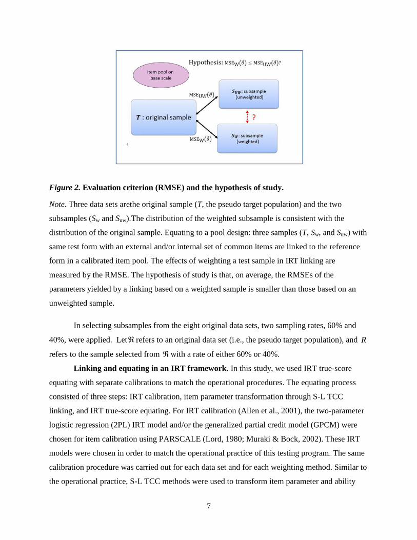
root of MSE (RMSE) was used as the evaluation criterion. Figure 2 presents the hypothesis of
study and the comparisons of the effects of linking based on weighted sample versus unweighted
sample.
Figure 1. Study design of the three samples employed in comparisons and the IRT linking
to a reference form in a calibrated item pool.
Note. Three data sets are original sample (T, the pseudo target population) and two subsamples
(Sw and Suw). The distribution of the weighted subsample is consistent with the distribution of the
original sample. Equating to a pool design: three samples (T, Sw, and Suw) with same test form
with an external and/or internal set of common items are linked to the reference form in a
calibrated item pool. The effects of weighting a test sample in IRT linking are measured by the
RMSE. The hypothesis is that, on average, the RMSEs of the parameters yielded by a linking
based on a weighted sample is smaller than those based on an unweighted sample.
7
Figure 2. Evaluation criterion (RMSE) and the hypothesis of study.
Note. Three data sets arethe original sample (T, the pseudo target population) and the two
subsamples (Sw and Suw).The distribution of the weighted subsample is consistent with the
distribution of the original sample. Equating to a pool design: three samples (T, Sw, and Suw) with
same test form with an external and/or internal set of common items are linked to the reference
form in a calibrated item pool. The effects of weighting a test sample in IRT linking are
measured by the RMSE. The hypothesis of study is that, on average, the RMSEs of the
parameters yielded by a linking based on a weighted sample is smaller than those based on an
unweighted sample.
In selecting subsamples from the eight original data sets, two sampling rates, 60% and
40%, were applied. Letℜ refers to an original data set (i.e., the pseudo target population), and R
refers to the sample selected from ℜwith a rate of either 60% or 40%.
Linking and equating in an IRT framework. In this study, we used IRT true-score
equating with separate calibrations to match the operational procedures. The equating process
consisted of three steps: IRT calibration, item parameter transformation through S-L TCC
linking, and IRT true-score equating. For IRT calibration (Allen et al., 2001), the two-parameter
logistic regression (2PL) IRT model and/or the generalized partial credit model (GPCM) were
chosen for item calibration using PARSCALE (Lord, 1980; Muraki & Bock, 2002). These IRT
models were chosen in order to match the operational practice of this testing program. The same
calibration procedure was carried out for each data set and for each weighting method. Similar to
the operational practice, S-L TCC methods were used to transform item parameter and ability
8
estimates of the new form to the scale of the reference forms or existing item pool based on
common items. The common items on the reference form are usually assembled from an item
pool already on the base scale.
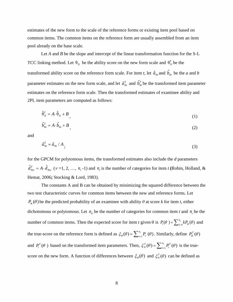
Let A and B be the slope and intercept of the linear transformation function for the S-L
TCC linking method. Let θN be the ability score on the new form scale and θTN be the
transformed ability score on the reference form scale. For item t, let ˆNta and ˆNtb be the a and b
parameter estimates on the new form scale, and let ˆTNta and ˆT
Ntb be the transformed item parameter
estimates on the reference form scale. Then the transformed estimates of examinee ability and
2PL item parameters are computed as follows:
ˆ ˆθ θTN NA B= ⋅ + , (1)
ˆ ˆTNt Ntb A b B= ⋅ + , (2)
and
ˆ ˆ /TNt Nta a A= ; (3)
for the GPCM for polytomous items, the transformed estimates also include the d parameters
ˆ ˆTNt Ntd A dν ν= ⋅ (ν =1, 2, …, nν -1) and nν is the number of categories for item t (Robin, Holland, &
Hemat, 2006; 9TStocking9T 9T& Lord, 19839T).
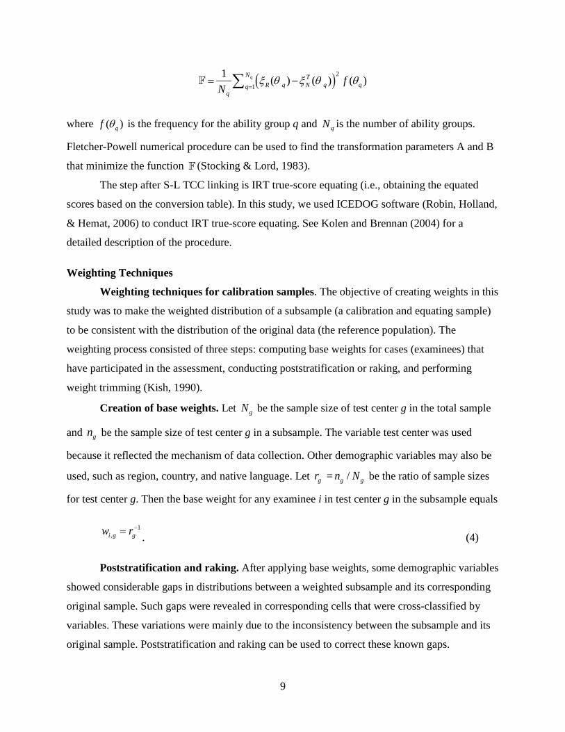
The constants A and B can be obtained by minimizing the squared difference between the
two test characteristic curves for common items between the new and reference forms. Let
( )tkP θ be the predicted probability of an examinee with ability θ at score k for item t, either
dichotomous or polytomous. Let tcn be the number of categories for common item t and cn be the
number of common items. Then the expected score for item t given θ is 0
( ) ( )tcnt tkk
P kPθ θ=
=∑ and
the true-score on the reference form is defined as 1
( ) ( )cnR tt
Pξ θ θ=
=∑ . Similarly, define ( )TtkP θ
and ( )TtP θ based on the transformed item parameters. Then,
1( ) ( )cnT T
N ttPξ θ θ
==∑ is the true-
score on the new form. A function of differences between ( )Rξ θ and ( )TNξ θ can be defined as
9
( )2
1
1 ( ) ( ) ( )qN TR q N q qq
q
fN
ξ θ ξ θ θ=
= −∑
where ( )qf θ is the frequency for the ability group q and qN is the number of ability groups.
Fletcher-Powell numerical procedure can be used to find the transformation parameters A and B
that minimize the function (Stocking & Lord, 1983).
The step after S-L TCC linking is IRT true-score equating (i.e., obtaining the equated
scores based on the conversion table). In this study, we used ICEDOG software (Robin, Holland,
& Hemat, 2006) to conduct IRT true-score equating. See Kolen and Brennan (2004) for a
detailed description of the procedure.
Weighting Techniques
Weighting techniques for calibration samples. The objective of creating weights in this
study was to make the weighted distribution of a subsample (a calibration and equating sample)
to be consistent with the distribution of the original data (the reference population). The
weighting process consisted of three steps: computing base weights for cases (examinees) that
have participated in the assessment, conducting poststratification or raking, and performing
weight trimming (Kish, 1990).
Creation of base weights. Let gN be the sample size of test center g in the total sample
and gn be the sample size of test center g in a subsample. The variable test center was used
because it reflected the mechanism of data collection. Other demographic variables may also be
used, such as region, country, and native language. Let gr = /g gn N be the ratio of sample sizes
for test center g. Then the base weight for any examinee i in test center g in the subsample equals
1,
−=i g gw r . (4)
Poststratification and raking. After applying base weights, some demographic variables
showed considerable gaps in distributions between a weighted subsample and its corresponding
original sample. Such gaps were revealed in corresponding cells that were cross-classified by
variables. These variations were mainly due to the inconsistency between the subsample and its
original sample. Poststratification and raking can be used to correct these known gaps.
10
Consequently, the linking based on the weighted sample will have improved precision such as
reduced mean squared error.
Poststratification adjustment matches the weighted sample cell counts to the population
cell counts by applying a proportional adjustment to the weights in each cell across the
contingency table (Cochran, 1977; Kish, 1965). Sometimes though, the sample can be spread too
thinly across the cells in the table, whereby poststratification would produce extreme weights in
cells with few cases and cause large design effects of weighting (Kish, 1965). To avoid such
flaws, raking is used to control marginal distributions for the variables of interest.
A raking procedure iteratively adjusts the case weights in the sample to make the
weighted marginal distribution of the sample agree with the marginal distribution of the
population on specified demographic variables (Deming, 1943). The algorithm used in raking is
called the Deming-Stephan algorithm (Deming & Stephan, 1940; Haberman, 1979). Again,
raking is conceptually similar to estimating the weights assigned to examinees or parameters
with a specified distribution of characteristics in an optimal sampling design, as described in
Berger (1997, pp. 73–75).
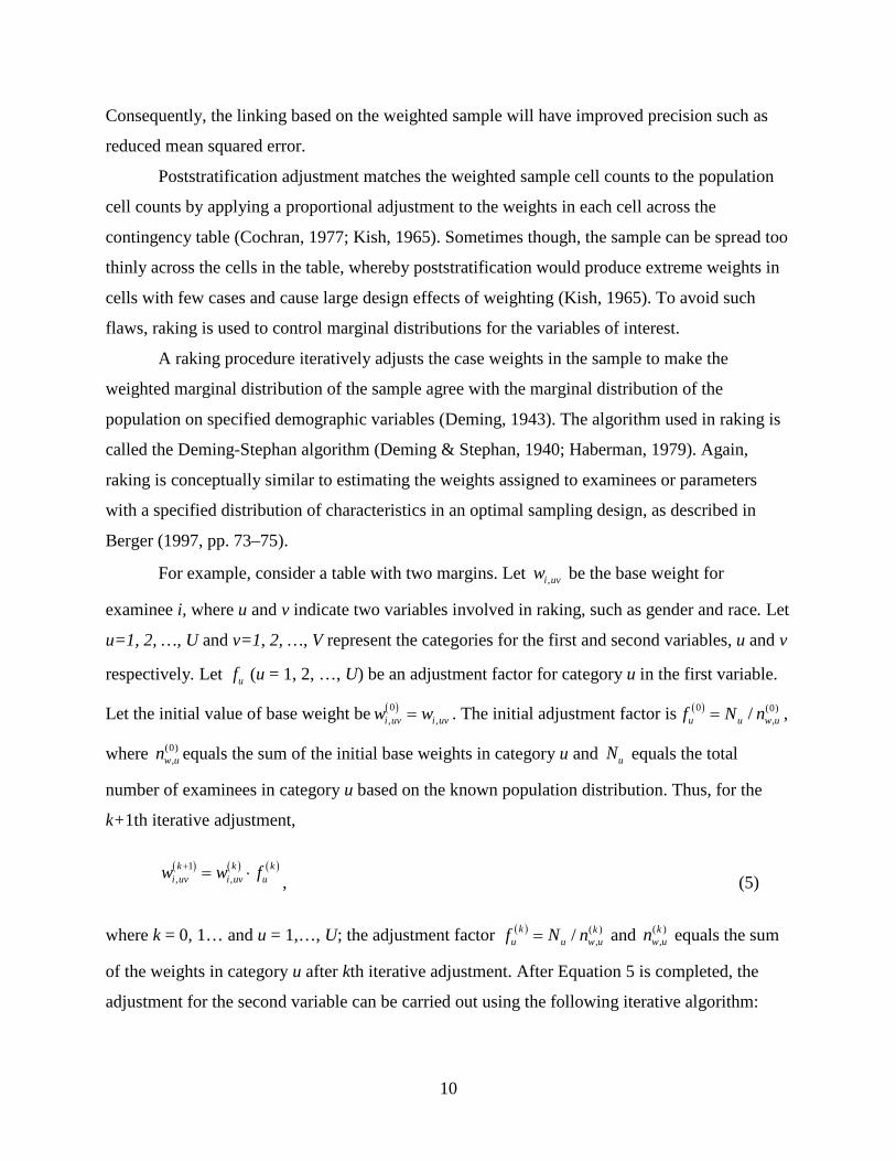
For example, consider a table with two margins. Let ,i uvw be the base weight for
examinee i, where u and v indicate two variables involved in raking, such as gender and race. Let
u=1, 2, …, U and v=1, 2, …, V represent the categories for the first and second variables, u and v
respectively. Let uf (u = 1, 2, …, U) be an adjustment factor for category u in the first variable.
Let the initial value of base weight be ( )0, ,=i uv i uvw w . The initial adjustment factor is ( )0 (0)
,/u u w uf N n= ,
where (0),w un equals the sum of the initial base weights in category u and uN equals the total
number of examinees in category u based on the known population distribution. Thus, for the
k+1th iterative adjustment,
( ) ( ) ( )1, ,k k k
i uv i uv uw w f+ = ⋅ , (5)
where k = 0, 1… and u = 1,…, U; the adjustment factor ( ) ( ),/k k
u u w uf N n= and ( ),k
w un equals the sum
of the weights in category u after kth iterative adjustment. After Equation 5 is completed, the
adjustment for the second variable can be carried out using the following iterative algorithm:

11
( ) ( ) ( )2 1 1, ,k k k
i uv i uv vw w f+ + += ⋅ , (6)
where ( )1+kvf (v = 1,…, V) is the adjustment factor for the second variable defined as
( ) ( )1 1,/+ +=k k
v v w vf N n where vN equals the total number of examinees in category v based on the
known population distribution and ( )1,+k
w vn equals the sum of base weights in category v after step k
+ 1 (k = 0, 1,…). The iterative procedure repeats the adjustment steps in Equations 5 and 6 until
the discrepancies between the weighted distribution and the population distribution meet the
predetermined criteria (i.e., considered as being converged) for each raking variable involved;
for example, repeating Equations 5 and 6 until step pk , such that ( ),any
max 0.01− ≤pku w uu
N n and
( ),any
max 0.01− ≤pkv w vv
N n . These are the optimality criteria of creating the weight for calibration
samples in this study. The raking algorithm normally converges, although the convergence speed
may be slow. Recently, log-linear models have been employed to implement the raking
adjustment because the main effects of log-linear models correspond to the given margins of the
contingency table. Thus, raking can be treated as fitting a main effects model (Haberman, 1979).
In this study, four demographic variables were used in the Deming-Stephan raking:
gender, age, time of language study, and reason for language study. As mentioned earlier, a total
of eight weights were formed by different raking schemes. The list of different sets of weights
used in this study is shown in the appendix.
Weight trimming. To reduce the design effects of weighting, the weight adjustment
process usually includes a weight trimming step (Liu, Ferraro, Wilson, & Brick, 2004). The
trimming process truncates extreme weights caused by unequal probability sampling or by raking
and poststratification adjustment. It reduces variation caused by extremely large weights but, at
the same time, may introduce some bias in estimation. Thus, the criterion of minimum mean
squared error is often employed in the trimming process (Potter, 1990). To investigate the effects
of different trimming criteria, though not optimal, we implemented three different criteria for
trimming the 60% subsamples and 10 criteria for the 40% subsamples. These trimming criteria
are given in the appendix.
Applying weights in calibration, linking, and equating. In the calibration step, weights
are applied to calibrate all the item responses based on 2PL IRT models using the PARSCALE.

12
Then, in the linking and scaling step, IRT linking is conducted based on the calibration output
using ICEDOG software. Finally, the conversion tables from the output of ICEDOG are used to
obtain equated true scores based on examinees’ observed scores.
Evaluation Criterion and Complete Grouped Jackknifing
In this study, we used both bias and the RMSE of linking parameters and equated scores
as the criteria to evaluate the effects of different weighting approaches. Bias measures the error
due to selection bias, and RMSE measures the overall variability due to both sampling and
selection bias. In general, RMSE is preferred to standard error or bias in evaluating the effects of
linking (van der Linden, 2010). In computing the RMSE, the original samples from the eight
administrations played the role of pseudo target populations, and the transformation parameters
yielded from the original samples were treated as the true values. A subsample was then
randomly selected from each original sample. Thus, it is viable to compare the RMSEs of the
parameter estimates from the weighted subsamples against those from the unweighted
subsamples. If the RMSEs of the linking parameter estimates for a weighted data set are smaller
than those for its unweighted counterpart, we can conclude that the weighted sample is closer to
its (pseudo) target population than the unweighted sample. Moreover, we also evaluated the
weighting effects on linking and equating by comparing the distributions of equated scores from
the weighted and unweighted subsamples against the distributions from the original sample (i.e.,
the pseudo target population). If the number of examinees with changes of scores from the
weighted subsample were found to be smaller than those from the unweighted subsample, then
the weighted linking process paid off. We expected that the linking results yielded from the
weighted samples would have smaller RMSEs and smaller seasonal effects than those from
unweighted samples.
To measure the errors of equating and linking procedures, both analytical and sampling
procedures have been proposed in the past (Braun & Holland, 1982; Kolen & Brennan, 2004;
Lord, 1982). In this study, resampling approaches, such as the jackknife repeated replication
(JRR) method (Quenouille, 1956; Tukey, 1958; Wolter, 1985), were used to estimate the
variances of the statistics of interest. The grouped jackknifing (GJRR) method is often used to
estimate the standard errors of the statistics of interest. Miller (1964) introduced a GJRR method
and derived its primary statistical theory. The JRR method was recently extended to evaluate the
variability of the estimates obtained from different samples through the whole equating

13
procedures, such as IRT calibration and S-L TCC linking (Haberman, Lee, & Qian, 2009). This
method, referred to as the complete grouped JRR (CGJRR) method, was applied in this study.
Because every CGJRR process comprised repetitions of both IRT calibration and the S-L TCC
linking procedure, the analysis conducted in this study was computationally intensive.
For comparison, the RMSEs of the estimated linking parameters were used to evaluate
the weighting effects on linking (i.e., checking whether a linking procedure was stable). A basic
task was, for weighted and unweighted subsamples, to estimate the bias and RMSE of the S-L
linking parameter estimates and score conversion at each raw score point. The estimation of
RMSE depended on the variance estimation of the statistics.
In this study, the CGJRR method was employed to estimate the standard errors of
statistics of interest (Qian, 2005). The CGJRR is based on jackknife replicate samples that are
formed by dropping a group of examinees from the whole sample R . Let J be the total number of
groups formed; J = 120 in this study. Let R be the whole sample employed in the study. We first
created 120 examinee groups with similar sizes by randomly assigning the examinees to these
groups. Compared with other grouping methods, the random grouping method often yields
appropriate results in CGJRR (Wang & Lee, 2012). In this study, none of the variables used to
create the weights was used as the basis for grouping. Let ( )jR (j = 1, 2, …, J) be the jth jackknife
replicate sample formed by dropping the jth group from the whole sample R ; hence, for this
study, a total of 120 jackknife replicate samples were formed. Following this, the CGJRR
procedure was used to estimate the variances of the statistics; through the entire process, the
same data set, either R or ( )jR , was used in the steps of both linking and estimation of the
statistics of interest. Let iy be the equated scale score for examinee i, which is transformed from
its raw score. Let Ry be the mean estimate from R . Let ( )jRy be the jackknife pseudo mean from
( )jR (j = 1, 2, …, J). The jackknifed variance of the mean estimate can be expressed as
( )( )( )2
*
1
1j
J
R R Rj
Jv y y yJ =
−= −∑
. (7)
The statistic involved in JRR could be in a very general form, rather than the simple
mean (e.g., a proportion, moments of different orders, and the transformation coefficients of the

14
S-L method). Let θ̂R be an estimate yielded from the whole sample and ( )
θ̂jR be the estimate
from the jth replicate sample through the complete jackknife procedure. Therefore, we can obtain
corresponding estimates of θ̂R such as the complete jackknifed variance, ( )θ̂Rv , and the mean
squared error, ( )ˆMSE θR .
For the linking based on a weighted sample wR , let θ̂wR be the estimate from wR . The
jackknifed variance of θ̂wR can be expressed as
( ) ( )( )2
1
1ˆ ˆ ˆθ θ θw ww j
J
R R Rj
JvJ =
−= −∑
. (8)
The MSE yielded by the results from the weighted subsample is
( ) ( ) ( )2ˆ ˆ ˆ ˆMSE θ θ θ θw w wR R Rv ℜ= + −
. (9)
The second term in Equation 9 is the estimate of squared bias. To evaluate the weighting effects
on linking for the study design, the MSE obtained from the weighted subsample, ( )ˆMSE θwR in
Equation 9, was compared with the corresponding MSE from the unweighted subsample,
( )ˆMSE θR .
Because each jackknife replicate sample must go through the whole equating process,
including the IRT calibration, the S-L TCC linking procedure and true-score equating, the
analysis requires intensive computation. Except for unweighted runs, each data set employs eight
raking schemes and 13 trimming criteria, and 120 JRR replications are carried out for each set of
weights. For the schemes of raking and trimming, see the appendix. In total, the study involved
more than 100,000 IRT equating linking processes. However, an application of weights to an
operational linking procedure is not computationally intensive; it only needs one additional step
of weight creation to the existing operations.
15
Results
Data Resources
In this study, we employed eight data sets from a large-scale international language
assessment, four from the reading section and four from the listening section; these assessments
were administered across different testing seasons. As described above, we created base weights
for each data set and applied raking and trimming techniques to the base weights. We also used
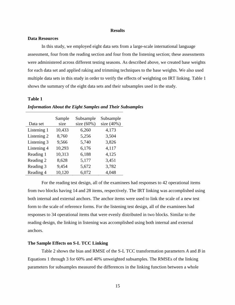
multiple data sets in this study in order to verify the effects of weighting on IRT linking. Table 1
shows the summary of the eight data sets and their subsamples used in the study.
Table 1
Information About the Eight Samples and Their Subsamples
Data set Sample
size Subsample size (60%)
Subsample size (40%)
Listening 1 10,433 6,260 4,173 Listening 2 8,760 5,256 3,504 Listening 3 9,566 5,740 3,826 Listening 4 10,293 6,176 4,117 Reading 1 10,313 6,188 4,125 Reading 2 8,628 5,177 3,451 Reading 3 9,454 5,672 3,782 Reading 4 10,120 6,072 4,048
For the reading test design, all of the examinees had responses to 42 operational items
from two blocks having 14 and 28 items, respectively. The IRT linking was accomplished using
both internal and external anchors. The anchor items were used to link the scale of a new test
form to the scale of reference forms. For the listening test design, all of the examinees had
responses to 34 operational items that were evenly distributed in two blocks. Similar to the
reading design, the linking in listening was accomplished using both internal and external
anchors.
The Sample Effects on S-L TCC Linking
Table 2 shows the bias and RMSE of the S-L TCC transformation parameters A and B in
Equations 1 through 3 for 60% and 40% unweighted subsamples. The RMSEs of the linking
parameters for subsamples measured the differences in the linking function between a whole

16
sample and its subsamples. Given that the theoretical value of B equals zero, the RMSEs of B
were sizable in the table, particularly for the 40% subsamples where these errors were non-
negligible. Moreover, on average, of the eight samples, the RMSEs of A and B were 20% and
41% larger, respectively, in the 40% subsamples than in the 60% subsamples. This evidence of
the sample variation effects signaled a need to reduce the variability in linking. The goal here
was to obtain a set of weights with RMSEs (for A and B or scale scores) that were smaller than
those from the unweighted data, as shown in Table 2.
Table 2
Bias and RMSE of the Estimated A and B for Subsamples (Unweighted)
Data set Whole
sample size Subsample
size A B
Bias RMSE Bias RMSE 60% subsample Listening 1 10,433 6,260 -0.0052 0.0155 0.0090 0.0177 Listening 2 8,760 5,256 0.0109 0.0221 -0.0045 0.0201 Listening 3 9,566 5,740 0.0188 0.0270 0.0101 0.0244 Listening 4 10,293 6,176 0.0153 0.0248 -0.0023 0.0187 Reading 1 10,313 6,188 -0.0018 0.0129 0.0213 0.0261 Reading 2 8,628 5,177 0.0064 0.0172 0.0037 0.0170 Reading 3 9,454 5,672 -0.0020 0.0186 0.0088 0.0227 Reading 4 10,120 6,072 -0.0064 0.0184 -0.0039 0.0186 40% subsample Listening 1 10,433 4,125 -0.0018 0.0168 0.0196 0.0268 Listening 2 8,760 3,451 0.0101 0.0254 0.0178 0.0304 Listening 3 9,566 3,782 0.0104 0.0262 0.0129 0.0287 Listening 4 10,293 4,048 -0.0033 0.0219 -0.0014 0.0235 Reading 1 10,313 4,173 0.0145 0.0214 0.0335 0.0383 Reading 2 8,628 3,504 -0.0224 0.0293 -0.0156 0.0250 Reading 3 9,454 3,826 -0.0143 0.0274 -0.0217 0.0339 Reading 4 10,120 4,117 -0.0020 0.0198 0.0123 0.0262
17
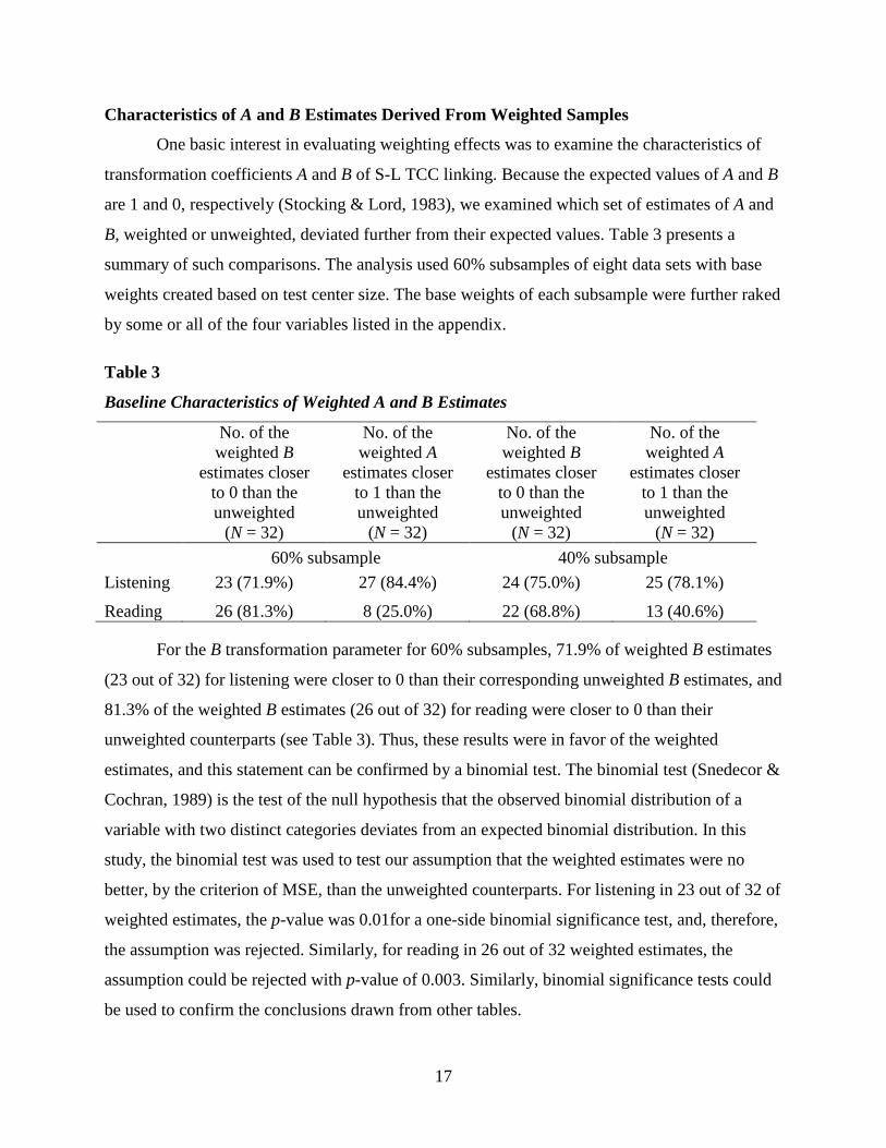
Characteristics of A and B Estimates Derived From Weighted Samples
One basic interest in evaluating weighting effects was to examine the characteristics of
transformation coefficients A and B of S-L TCC linking. Because the expected values of A and B
are 1 and 0, respectively (Stocking & Lord, 1983), we examined which set of estimates of A and
B, weighted or unweighted, deviated further from their expected values. Table 3 presents a
summary of such comparisons. The analysis used 60% subsamples of eight data sets with base
weights created based on test center size. The base weights of each subsample were further raked
by some or all of the four variables listed in the appendix.
Table 3
Baseline Characteristics of Weighted A and B Estimates
No. of the weighted B
estimates closer to 0 than the unweighted
(N = 32)
No. of the weighted A
estimates closer to 1 than the unweighted
(N = 32)
No. of the weighted B
estimates closer to 0 than the unweighted
(N = 32)
No. of the weighted A
estimates closer to 1 than the unweighted
(N = 32) 60% subsample 40% subsample Listening 23 (71.9%) 27 (84.4%) 24 (75.0%) 25 (78.1%)
Reading 26 (81.3%) 8 (25.0%) 22 (68.8%) 13 (40.6%)
For the B transformation parameter for 60% subsamples, 71.9% of weighted B estimates
(23 out of 32) for listening were closer to 0 than their corresponding unweighted B estimates, and
81.3% of the weighted B estimates (26 out of 32) for reading were closer to 0 than their
unweighted counterparts (see Table 3). Thus, these results were in favor of the weighted
estimates, and this statement can be confirmed by a binomial test. The binomial test (Snedecor &
Cochran, 1989) is the test of the null hypothesis that the observed binomial distribution of a
variable with two distinct categories deviates from an expected binomial distribution. In this
study, the binomial test was used to test our assumption that the weighted estimates were no
better, by the criterion of MSE, than the unweighted counterparts. For listening in 23 out of 32 of
weighted estimates, the p-value was 0.01for a one-side binomial significance test, and, therefore,
the assumption was rejected. Similarly, for reading in 26 out of 32 weighted estimates, the
assumption could be rejected with p-value of 0.003. Similarly, binomial significance tests could
be used to confirm the conclusions drawn from other tables.

18
For the A transformation parameter for the 60% subsamples, 84.4% of weighted A
estimates for listening were closer to 1 than corresponding unweighted ones. However, the
weighted A estimates from the reading test did not show the same characteristics. We analyzed
different A parameter estimates from the reading data and found that when the unweighted
estimates from a subsample were closer to 1 than the estimates from the original sample, the
weighted estimates from the subsample could actually be closer to the estimates from the original
sample than 1. This is, in fact, consistent with weighting principles. Similar results are shown in
the second part of Table 3 for the 40% subsample.
Comparison of the A and B Estimates for Weighted and Unweighted Subsamples
To evaluate weighting effects, we also compared the biases and RMSEs of A and B for
the weighted and the unweighted subsamples (60% and 40%); Table 4 contains the results of the
comparisons. The base weights were created based on test center sizes with raking. For each
listening or reading subsample, all eight sets of weights listed in the appendix were used in the
analysis. The results are shown in Table 4.
Table 4
Comparison of the Bias and RMSEs of the Weighted A and B Estimates With Those of the
Unweighted Ones
No. of the bias of weighted B
smaller than the unweighted
(N = 32)
No. of the RMSE of weighted B
smaller than the unweighted
(N = 32)
No. of the bias of weighted A
smaller than the unweighted
(N = 32)
No. of the RMSE of weighted A
smaller than the unweighted
(N = 32) 60% subsample Listening 16 (50.0%) 16 (50.0%) 28 (87.5%) 16 (50.0%) Reading 22 (68.8%) 22 (68.8%) 20 (62.5%) 20 (62.5%)
40% subsample
Listening 32 (100.0%) 32 (100.0%) 24 (75.0%) 32 (100.0%)
Reading 32 (100.0%) 32 (100.0%) 28 (87.5%) 28 (87.5%)
For the 60% reading subsamples, 68.8% of the biases and RMSEs of the B parameter
estimates (22 out of 32) obtained from the weighted samples were smaller than those estimated
from the unweighted samples. For A parameter estimates, 62.5% of their bias and RMSE
19
estimates (20 out of 32) obtained from weighted samples were smaller than those estimated from
the unweighted samples.
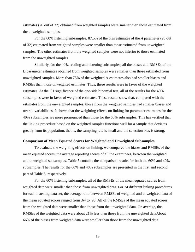
For the 60% listening subsamples, 87.5% of the bias estimates of the A parameter (28 out
of 32) estimated from weighted samples were smaller than those estimated from unweighted
samples. The other estimates from the weighted samples were not inferior to those estimated
from the unweighted samples.
Similarly, for the 40% reading and listening subsamples, all the biases and RMSEs of the
B parameter estimates obtained from weighted samples were smaller than those estimated from
unweighted samples. More than 75% of the weighted A estimates also had smaller biases and
RMSEs than those unweighted estimates. Thus, these results were in favor of the weighted
estimates. At the .01 significance of the one-side binomial test, all of the results for the 40%
subsamples were in favor of weighted estimates. These results show that, compared with the
estimates from the unweighted samples, those from the weighted samples had smaller biases and
overall variabilities. It shows that the weighting effects on linking for parameter estimates for the
40% subsamples are more pronounced than those for the 60% subsamples. This has verified that
the linking procedure based on the weighted samples functions well for a sample that deviates
greatly from its population, that is, the sampling rate is small and the selection bias is strong.
Comparison of Mean Equated Scores for Weighted and Unweighted Subsamples
To evaluate the weighting effects on linking, we compared the biases and RMSEs of the
mean equated scores, the average reporting scores of all the examinees, between the weighted
and unweighted subsamples. Table 5 contains the comparison results for both the 60% and 40%
subsamples. The results for the 60% and 40% subsamples are presented in the first and second
part of Table 5, respectively.
For the 60% listening subsamples, all of the RMSEs of the mean equated scores from
weighted data were smaller than those from unweighted data. For 24 different linking procedures
for each listening data set, the average ratio between RMSEs of weighted and unweighted data of
the mean equated scores ranged from .64 to .93. All of the RMSEs of the mean equated scores
from the weighted data were smaller than those from the unweighted data. On average, the
RMSEs of the weighted data were about 21% less than those from the unweighted dataAbout
66% of the biases from weighted data were smaller than those from the unweighted data.
20
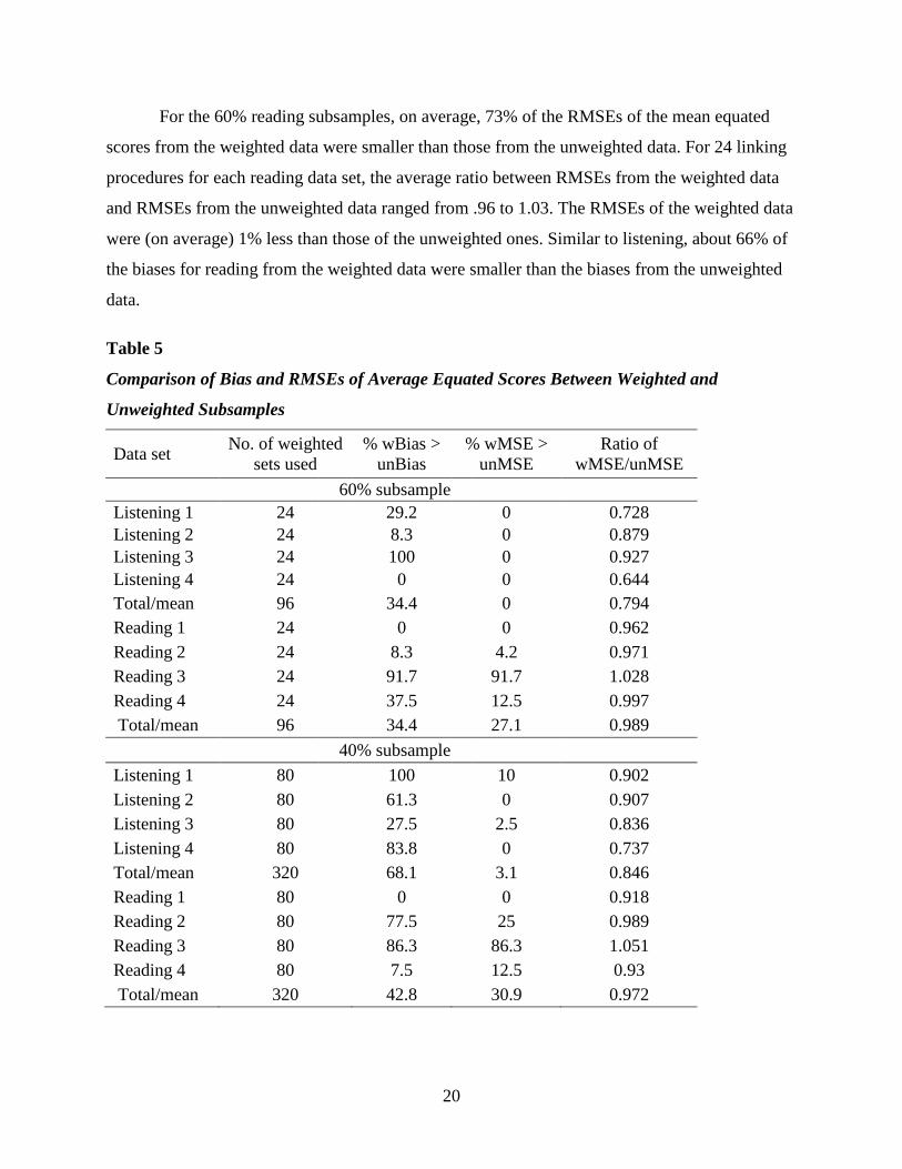
For the 60% reading subsamples, on average, 73% of the RMSEs of the mean equated
scores from the weighted data were smaller than those from the unweighted data. For 24 linking
procedures for each reading data set, the average ratio between RMSEs from the weighted data
and RMSEs from the unweighted data ranged from .96 to 1.03. The RMSEs of the weighted data
were (on average) 1% less than those of the unweighted ones. Similar to listening, about 66% of
the biases for reading from the weighted data were smaller than the biases from the unweighted
data.
Table 5
Comparison of Bias and RMSEs of Average Equated Scores Between Weighted and
Unweighted Subsamples
Data set No. of weighted sets used
% wBias > unBias
% wMSE > unMSE
Ratio of wMSE/unMSE
60% subsample Listening 1 24 29.2 0 0.728 Listening 2 24 8.3 0 0.879 Listening 3 24 100 0 0.927 Listening 4 24 0 0 0.644 Total/mean 96 34.4 0 0.794 Reading 1 24 0 0 0.962 Reading 2 24 8.3 4.2 0.971 Reading 3 24 91.7 91.7 1.028 Reading 4 24 37.5 12.5 0.997 Total/mean 96 34.4 27.1 0.989 40% subsample Listening 1 80 100 10 0.902 Listening 2 80 61.3 0 0.907 Listening 3 80 27.5 2.5 0.836 Listening 4 80 83.8 0 0.737 Total/mean 320 68.1 3.1 0.846 Reading 1 80 0 0 0.918 Reading 2 80 77.5 25 0.989 Reading 3 80 86.3 86.3 1.051 Reading 4 80 7.5 12.5 0.93 Total/mean 320 42.8 30.9 0.972

21
For the 40% subsamples, data set for either listening or reading, 80 different sets of
weights in linking were applied to each data set. For the listening data, 97% of the RMSEs from
weighted data were smaller than those from unweighted data. For the 40% listening subsamples,
on average, the RMSEs from weighted data were about 15% less than those from the unweighted
data. About 32% of the biases from weighted data were smaller than those from unweighted
data.
For the 40% reading subsamples, 69% of the RMSEs of the mean equated scores from
weighted data were smaller than those from unweighted data. The weighted RMSEs were (on
average) 3% less than those from the unweighted data. About 57% of the biases from the
weighted data were smaller than those from the unweighted data. Using a binomial test at the .01
level, all of the results, except for reading data set 3, were significantly in favor of the weighted
estimates.
Comparison of the Distributions of Scores Between Weighted and Unweighted Subsamples
Table 6 contains a comparison of the distributions of equated scores change of weighted
and unweighted subsamples, for both 60% and 40% sampling rates. Using the original sample
results as the criteria, the percentage of examinees whose equated scores changed under the
weighted or unweighted subsample is shown in Table 6. Here, the magnitude of the changes in
percentage measures the stability of linking. The smaller the percentage, the more stable a
linking. Although several comparable raking schemes (see the appendix) were applied to each set
of base weights, no differences were found in the distributions of equated scores across weights
by different raking schemes. However, differences were found in the distributions of equated
scores between weighted and unweighted subsamples. This indicates that the weighting
techniques are reasonably robust in IRT true-score equating.
For the 60% listening subsample, the percentage of examinees whose equated scores
differed from the original data was 1.2% for the weighted data and 1.6% for the unweighted data.
For the 60% reading subsample, the corresponding score change percentages (weighted vs.
unweighted) were 1.4% and 2.9%, respectively.
For the 40% listening subsample, the percentage of examinees who had their equated
scores changed from the original data was 1.2% for the weighted data, as opposed to 2.7% for
the unweighted data. For the 40% reading subsample, the corresponding score change
percentages (weighted vs. unweighted) were 1.4% and 3.0%, respectively. On average, the

22
percentage of examinees having their scores changed in the unweighted sample is about twice
that of examinees in the weighted sample. The strategy of weighting aligns the proportions of the
examinee groups of interest in the sample to those in the target population. Linking through a
weighted sample shows a higher likelihood for examinees with the same response pattern to be
assigned the same equated scores as in the total sample. The results in Table 6 directly show the
stability of the linking employing weighted samples.
Table 6
Comparison of Distributions of Equated Scores Between Weighted and Unweighted
Subsamples
Data set Weighted Unweighted
No. of cases changed score
% changed score
No. of cases changed score
% changed score
60% subsample Listening 1 109 1.74 0 0 Listening 2 0 0 98 1.86 Listening 3 43 0.75 43 0.75 Listening 4 138 2.23 237 3.84 Mean 72.5 1.2 94.5 1.6 Reading 1 75 1.21 233 3.77 Reading 2 168 3.25 347 6.7 Reading 3 72 1.27 72 1.27 Reading 4 0 0 0 0 Mean 78.8 1.4 163 2.9 40% subsample Listening 1 73 1.75 73 1.75 Listening 2 0 0 59 1.68 Listening 3 35 0.91 115 3.01 Listening 4 94 2.28 182 4.42 Mean 50.5 1.2 107.3 2.7 Reading 1 50 1.21 62 1.5 Reading 2 108 3.13 267 7.74 Reading 3 51 1.35 51 1.35 Reading 4 0 0 57 1.41 Mean 52.3 1.4 109.3 3.0

23
Discussion
This study explored the use of weighting techniques to achieve a more stable calibration,
linking and equating procedures across administrations. In the method proposed here, the
weighted distributions of the administrations would be consistent as if all of them were randomly
sampled from the target population. In this way, a sampling scheme over numerous
administrations is designed.
There are four major contributions of this study: (a) a discussion of the necessity of
determining an improved sampling design over time for assessments with complex equating
designs; (b) an introduction of weighting techniques to construct improved samples for
calibration, linking, and equating; (c) an explicit way to evaluate the weighting effects on linking
for the new design through the comparison of the results yielded by weighted subsamples with
those by unweighted subsamples; and (d) a practically feasible and easy application to
implement the weighting techniques in a large-scale testing program with numerous
administrations per year.
The results showed that the proposed paradigm in this paper was an effective method for
evaluating the use of weighting techniques to increase the precision in linking procedures.
Although this analysis involved reducing the variability across multiple samples, the evaluation
methodology can certainly be employed to analyze weighting technique to investigate the
precision of item calibration through item selection. Thus, we think, this procedure may also be
used for constructing a better test design.
Application has always been a focus of this study. The proposed weighting strategy can
be employed in two scenarios. First, applying the strategy in an assessment with multiple forms,
such as GRE and TOEFL, with variability and seasonality among multiple test samples. Second,
applying the strategy in analyzing partial data. A typical example is analyzing the data from state
assessments where the available data for making initial linking decisions are usually only about
20% of the final data. Instead of using randomization, the initial data are often a convenient
sample gathered from well-organized school districts. So applying weighting techniques could
help psychometricians avoid biased results based on the initial equating analysis. Note that if the
initial sample of a state assessment is randomized, the problem might be less significant. In
general, the weighting procedure can be used to correct the disagreements between a sample and
its population, such as under- or overrepresentation of certain subgroups for a given

24
administration. Moreover, applying weighting techniques, including creating weights and raking,
is not very complex, although evaluating weighting efficiency as done in this study is
computationally intensive.
For future research, we may consider a different strategy, such as imposing selection bias
in samples by deliberately oversampling certain demographic groups to evaluate the effects of
optimized weighting on reducing selection bias. In another future research direction, we may
conduct a comparison of the method that we proposed here to the formal optimal sampling
design described by Berger (1997). The difficulty in following Berger’s approach consists of
formally modeling the various aspects of the situation: the background information, the IRT
model parameters for each administration, the IRT linking parameter for each pair of
administrations, and all these aspects for multiple test forms/administrations. In this research
direction, we might first focus on linking only two test forms/administrations, in a simple way,
such as using a mean-mean IRT linking. The formal expression of the IRT linking expressed as a
restriction function on the parameter space as given in von Davier and von Davier (2011) could
be useful for writing the constraints formally. As in von Davier and von Davier (2011) and using
the definition of an optimal sampling design (Berger, 1991, 1997), suppose two tests X and Y
were taken by n examinees, for which we assume a distribution of ability θ and a multivariate
distribution of relevant background variables. Corresponding to each value of θ, there is a weight
w associated with the background variables. Then according to Berger (1997), a sampling design
with pair (θ, w) is locally optimal if a specific optimality criterion (which is usually a function of
the information matrix) is achieved. Writing the linking parameters as constraints as in von
Davier and von Davier (2011) might aid with writing the constraints formally in the linear
programming for estimating the weights that lead to a sample for which the linking parameters
are estimated most efficiently.
25
References
Allen, N., Donoghue, J., & Schoeps, T. (2001). The NAEP 1998 technical report (NCES 2001-
509). Washington, DC: National Center for Education Statistics.
Berger, M. P. F. (1991). On the efficiency of IRT models when applied to different sampling
designs. Applied Psychological Measurement, 15, 293–306.
Berger, M. P. F. (1997). Optimal designs for latent variable models: A review. In J. Rost & R.
Langeheine (Eds.), Application of latent trait and latent class models in the social
sciences (pp. 71–79). Muenster, Germany: Waxmann.
Berger, M. P. F., King, C. Y. J., & Wong, W. K. (2000). Minimax D-optimal designs for item
response theory models. Psychometrika, 65, 377–390.
Berger, M. P. F., & van der Linden, W. J. (1992). Optimality of sampling designs in item
response theory models. In M. Wilson (Ed.), Objective measurement: Theory into
practice (Vol. 1, pp. 274–288). Norwood, NJ: Ablex.
Braun, H. I., & Holland, P. W. (1982). Observed-score test equating: A mathematical analysis of
some ETS equating procedures. In P. W. Holland & D. B. Rubin (Eds.), Test equating
(pp. 9–49). New York, NY: Academic Press.
Buyske, S. (2005). Optimal design in educational testing. In M. P. F. Berger & W. K. Wong
(Eds.), Applied optimal designs (pp. 1–19). New York, NY: John Wiley & Sons.
Cochran, W. G. (1977). Sampling techniques (3rd ed.). New York, NY: John Wiley & Sons.
Deming, W. E. (1943). Statistical adjustment of data. New York, NY: Wiley.
Deming, W. E., & Stephan, F. F. (1940). On a least squares adjustment of a sampled frequency
table when the expected marginal tables are known. Annals of Mathematical Statistics,
11, 427–444.
Dorans, N. J., & Holland, P. W. (2000). Population invariance and equitability of tests: Basic
theory and the linear case. Journal of Educational Measurement, 37, 281–306.
Duong, M., & von Davier, A. A. (2012). Observed-score equating with a heterogeneous target
population. International Journal of Testing, 12, 224–251.
Guo, H., Liu, J., Haberman, S., & Dorans, N. (2008, March). Trend analysis in seasonal time
series models. Paper presented at the annual meeting of the National Council on
Measurement in Education, New York, NY.
Haberman, S. J. (1979). Analysis of qualitative data (Vol. 2). New York, NY: Academic Press.

26
Haberman, S. J., Lee, Y., & Qian, J. (2009). Jackknifing techniques for evaluation of equating
accuracy (ETS Research Report No. RR-09-39). Princeton, NJ: Educational Testing
Service.
Holland, P. W. (2007). A framework and history for score linking. In N. J. Dorans, M.
Pommerich, & P. W. Holland (Eds.), Linking and aligning scores and scales (pp. 5–30).
New York, NY: Springer-Verlag.
Huggins, A. C. (2011, April). Equating invariance across curriculum groups on a statewide
fifth-grade science exam. Paper presented at the annual meeting of the American
Educational Research Association, New Orleans, LA.
Jones, D. H., & Jin, Z. (1994). Optimal sequential designs for on-line item estimation.
Psychometrika, 59, 59–75.
Kish, L. (1965). Survey sampling. New York, NY: John Wiley & Sons.
Kish, L. (1990). Weighting: Why, when, and how? In Proceedings of the Joint Statistical
Meetings, Section on Survey Research Methods (pp. 121–129). Alexandria, VA:
American Statistical Association.
Kolen, M. J. (2004). Population invariance in equating and linking: Concept and history. Journal
of Educational Measurement, 41, 3–14.
Kolen, M. J., & Brennan, R. L. (2004). Test equating, scaling, and linking: Methods and
practices (2nd ed.). New York, NY: Springer-Verlag.
Lee, Y., & von Davier, A. A. (2013). Monitoring scale scores over time via quality control
charts, model-based approaches, and time series techniques. Psychometrika, 78, 557–575.
Li, D., Li, S., & von Davier, A. A. (2011). Applying time-series analysis to detect scale drift. In
A. A. von Davier (Ed.), Statistical models for test equating, scaling, and linking (pp.
381–398). New York, NY: Springer.
Liu, B., Ferraro, D., Wilson, E., & Brick, M. J. (2004). Trimming extreme weights in household
surveys. Proceedings of the Joint Statistical Meetings, Section on Survey Research
Methods (pp. 3905–3912). Alexandria, VA: American Statistical Association.
Livingston, S. A. (2004). Equating test scores (without IRT). Princeton, NJ: Educational Testing
Service.
Livingston, S. A. (2007). Demographically adjusted groups for equating test scores.
Unpublished manuscript.

27
Lord, F. M. (1980). Applications of item response theory to practical testing problems. Hillsdale,
NJ: Erlbaum.
Lord, F. M. (1982). The standard error of equipercentile equating. Journal of Educational
Statistics, 7, 165–174.
Lord, M. F., & Wingersky, M. S. (1985). Sampling variances and covariances of parameter
estimates in item response theory. In D. J. Weiss (Ed.), Proceedings of the 1982 IRT/CAT
Conference. Minneapolis: University of Minnesota, Department of Psychology, CAT
Laboratory.
Miller, R. G. (1964). A trustworthy jackknife. Annals of Mathematical Statistics, 53, 1594–1605.
Moses, T. (2011). Evaluating empirical relationships among prediction, measurement, and
scaling invariance (ETS Research Report No. RR-11-06). Princeton, NJ: Educational
Testing Service.
Muraki, E., & Bock, R. D. (2002). PARSCALE (Version 4.1) [Computer software].
Lincolnwood, IL: Scientific Software International.
Neidorf, T.S., Binkley, M., Gattis, K., & Nohara, D. (2006). Comparing mathematics content in
the National Assessment of Educational Progress (NAEP), Trends in International
Mathematics and Science Study (TIMSS), and Programme for International Student
Assessment (PISA) 2003 Assessments (NCES 2006-029). Washington, DC: US
Department of Education, National Center for Education Statistics.
Nohara, D. (2001). A Comparison of the National Assessment of Educational Progress (NAEP),
the Third International Mathematics and Science Study Repeat (TIMSS-R), and the
Programme for International Student Assessment (PISA) (NCES 2001-07). Washington,
DC: US Department of Education, National Center for Education Statistics.
Potter, F. J. (1990). A study of procedures to identify and trim extreme sampling weights.
Proceedings of the section on survey research methods (pp. 225–230). Alexandria, VA:
American Statistical Association.
Qian, J. (2005, April). Measuring the cumulative linking errors of NAEP trend assessments.
Paper presented at the annual meeting of the National Council on Measurement in
Education, Montreal, Canada.

28
Qian, J. (2012, April). Updating the empirical target population in weighted IRT equating. Paper
presented at the annual meeting of the National Council on Measurement in Education,
Vancouver, Canada.
Qian, J., von Davier, A., & Jiang, Y. (2013). Achieving a stable scale for an assessment with
multiple forms: weighting test samples in IRT linking and equating. In R. E. Millsap, L.
A. van der Ark, D. M. Bolt, & C. M. Woods (Eds.), New developments in quantitative
psychology: Presentations from the 77th annual Psychometric Society meeting (pp. 171–
185). New York, NY: Springer.
Quenouille, M. H. (1956). Notes on bias in estimation. Biometrika, 43, 353–360.
Robin, F., Holland P., & Hemat, L. (2006). ICEDOG [Computer software]. Princeton, NJ:
Educational Testing Service.
Sinharay, S., Holland, P. W., von Davier, A. A. (2011). Evaluating the missing data assumptions
of the chain and poststratification equating methods. In A. A. von Davier (Ed.), Statistical
models for test equating, scaling, and linking (pp. 381–398). New York, NY: Springer.
Snedecor, G. W., & Cochran, W. G. (1989). Statistical methods (8th ed.). Ames, IA: Iowa State
University Press.
Stocking, M. L. (1990). Specifying optimum examinees for item parameter estimation in item
response theory. Psychometrika, 55, 461–475.
Stocking, M. L., & Lord, F. M. (1983). Developing a common metric in item response theory.
Applied Psychological Measurement, 7, 201–210.
Tukey, J. (1958). Bias and confidence in not quite large samples. Annals of Mathematical
Statistics, 29, 614.
Turner, R., & Adams, R. J. (2007). The Program for International Student Assessment: An
overview. Journal of Applied Measurement, 8, 237–248.
van der Linden, W. J. (2010). On bias in linear observed-score equating. Measurement, 8, 21–26.
van der Linden, W. J., & Luecht, R. M. (1998). Observed-score equating as a test assembly
problem. Psychometrika, 63, 401–418.
von Davier, A. A., Holland, P. W., & Thayer, D. T. (2004). The chain and post-stratification
methods for observed-score equating and their relationship to population invariance.
Journal of Educational Measurement, 41, 15–32.
29
von Davier, A. A., & Wilson, C. (2008). Investigating the population sensitivity assumption of
item response theory true-score equating across two subgroups of examinees and two test
formats. Applied Psychological Measurement, 32, 11–26.
von Davier, M., & von Davier, A. A. (2011). A general model for IRT scale linking and scale
transformation. In A. A. von Davier (Ed.), Statistical models for test equating, scaling,
and linking (pp. 225–242). New York, NY: Springer9T
.
Wang, L., & Lee, Y. (2012). Effects of random and cluster-based groupings on grouped
jackknife variance estimation for IRT true score equating. Unpublished manuscript.
Wolter, K. (1985). Introduction to variance estimation. New York, NY: Springer.
Yang, W. L., & Gao, R. (2008). Invariance of score linkings across gender groups for forms of a
testlet-based college-level examination program examination. Applied Psychological
Measurement, 32, 45–61.
Yi, Q., Harris, D. J., & Gao, X. (2008). Invariance of equating functions across different
subgroups of examinees taking a science achievement test. Applied Psychological
Measurement, 32, 62–80.
Zumbo, B. D. (2007). Validity: foundational issues and statistical methodology. In C. R. Rao &
S. Sinharay (Eds.), Handbook of statistics: Vol. 26. Psychometrics (pp. 45–79). The
Netherlands: Elsevier Science B.V.

30
Notes 1 We have also been inspired by other lines of work. We will provide the references for these
works accordingly in the text. Some of these are sampling procedures in survey assessment
and poststratification equating.

31
Appendix
Weights, Raking Variables, and Number of Trimming Criteria Applied in Analyses
Weight
Variable used
for base weight
Variables used
for rakinga
Criteria used for trimminga
60%
subsample
40%
subsample
W0A Test center V1, V2, V3, V4 3 10
W0B Test center V1, V2, V3 3 10
W0C Test center V1, V2 3 10
W0YY Test center V1, V3 3 10
W0ZZ Test center V2, V3 3 10
W0X Test center V1 3 10
W0Y Test center V2 3 10
W0Z Test center V3 3 10
Note. V1 = gender, V2 = age, V3 = time of language study, V4 = reason for language study. a In trimming, the total of the weights was normalized to the size of each subsample. The default
trimming criterion was set at 2. For the base weights based on test center, the criteria used for
trimming of the 60% subsamples: 1.7, 1.85, and 2; the criteria for the 40% subsamples: ranged
from 1.5 to 2.4 with an even interval of 0.1. The base weights based on native language only
used the default trimming criterion.


