
WHAT IS EXCEL, AND WHY DO WE USE IT?
Excel is a spreadsheet program that allows you to
store, organize, and analyze information
Descriptives: For continuous variables, displays mean, median, mode,
minimum/maximum, and range.
Frequencies: For categorical variables, displays percentages, distributions,
Skewness
Tables/Graphs
Storing, Sorting, Recoding, Manipulating, Cleaning Data
Calculations & Formulas

EXCEL BASICS: ROWS, COLUMNS, AND CELLS
Rows: each numbered
along the left side of
the spreadsheet
Columns: labeled with letters along the top part of
the spreadsheet.Cells: each cell is
represented by a
rectangular box. Currently
only cell A1 is selected.
Multiple cells can be
selected by clicking and
dragging the selected
cell.

EXCEL BASICS: SUMS AND AVERAGES
• We will use the following hypothetical sample of Oxy students and calculate the total money
earned on campus, and the average GPA.

EXCEL BASICS: SUMS AND AVERAGES
• To find the sum, start by typing “=sum” below the column of numbers you want to
add together. Next, select the range of numbers you want the sum of (blue
rectangular box)

EXCEL BASICS: SUMS AND AVERAGES• To find the average GPA, type “=average” and again select the numbers you want to
average with the blue rectangular box

EXCEL BASICS: MINIMUM AND MAXIMUM
• To find the minimum or maximum in a set of numbers, repeat the same process
except type “=min” or “=max”

EXCEL BASICS: QUARTILES
• When calculating quartiles for a range of number, you can choose
exactly which quartile you want displayed, notated by a 1, 2, or 3.
Note that after you select your range of number, you must use a
comma followed by a space then a number.

EXCEL BASICS: SORTING
• Excel’s ability to sort is invaluable when you need to
focus on particular areas and organize your data.
• In our example, we will sort by sex, then by GPA
• The first step to sorting your data is selecting your
entire dataset, then clicking DataSort
EXCEL BASICS: SORTING
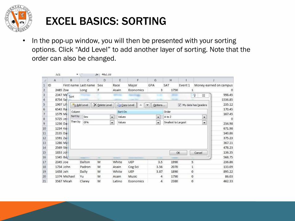
• In the pop-up window, you will then be presented with your sorting
options. Click “Add Level” to add another layer of sorting. Note that the
order can also be changed.

EXCEL BASICS: SORTING
• These data are sorted by sex first, then ascending GPA
EXCEL BASICS: CONCATENATE
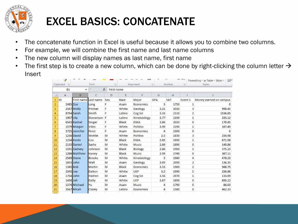
• The concatenate function in Excel is useful because it allows you to combine two columns.
• For example, we will combine the first name and last name columns
• The new column will display names as last name, first name
• The first step is to create a new column, which can be done by right-clicking the column letter
Insert

EXCEL BASICS: CONCATENATE
• In the new column, type
“=concatenate” then select the two
cells that you want to combine
• In this example, a comma between
the two names is created by typing
(D2,”, “,C2)
• Double-click the bottom right
corner of the cell to fill the formula
down through the column

• Text to Columns is the opposite of concatenate – it splits data
apart, either at a fixed point in the data, or based on a
delimiter (space, comma, etc.)
• Go to Data>Text to Columns
TEXT TO COLUMNS
Note: you typically
want to select
delimited. Any
words separated by
commas or spaces
fall under this
category.

TEXT TO COLUMNS • In this case, the
names were
separated by a
comma.
• Now, the last names
and first names
appear in two
different columns

CREATING AND INTERPRETING PIVOTTABLES
• PivotTables are one of Excel’s most powerful functions.
• Allow you to pick and choose the variables you want to compare.
• Make meaningful interpretations from your data.
• To make your PivotTable, select your data then click insertPivotTable
• Create a unique identifier for each case, if not already present (such as
A# or PIDM)
• Insert>New Column>“UniqueID”>Autofill with increasing numbers
• This will be your count variable
CREATING AND INTERPRETING PIVOTTABLES
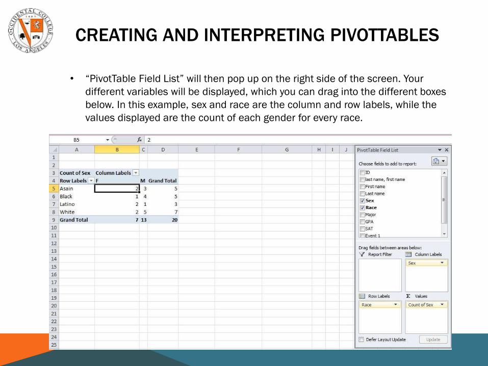
• “PivotTable Field List” will then pop up on the right side of the screen. Your
different variables will be displayed, which you can drag into the different boxes
below. In this example, sex and race are the column and row labels, while the
values displayed are the count of each gender for every race.

CREATING AND INTERPRETING PIVOT TABLES
Column Percent
Row Percent
• To find your column percent, right-click one of
your values and select show values as% of
column total
• These numbers tell you what percent of each
gender are Asian, Black, Latino, etc.
• For example, you can conclude that 28.57% of
females are Asian
• To find your row percent, right-click one of your values
and select show values as% of row total
• These numbers tell you what percent of each race are
male or female
• For example, you can conclude that 40% of Asians are
female
Note: Row and Column percent are
only used with categorical variables

FORMATTING NUMBERS IN PIVOTTABLES
• To format numbers in PivotTables, right-click on one of your numbers, then
go to number format.
• On the pop-up menu, you can select the number of decimal places you want
displayed which will apply to every number in your PivotTable.
Right-click

CREATING A PIVOTCHART FROM A PIVOTTABLE
• The first step to creating a PivotChart is dragging
the desired variables into the appropriate areas on
the PivotTable Field list. Once your PivotTable
appears, click on it, then go to Insert and select
your desired chart type. In this case, we will use a
2D bar chart.

CREATING A PIVOTCHART FROM A PIVOTTABLE
• Once your PivotChart appears, you can add features to make your chart
more complete. On the Layout tab, you can add a Chart Title, Data Labels
and Axis Titles. On the Design tab, you can click different chart layouts to
change the feel of your PivotChart.
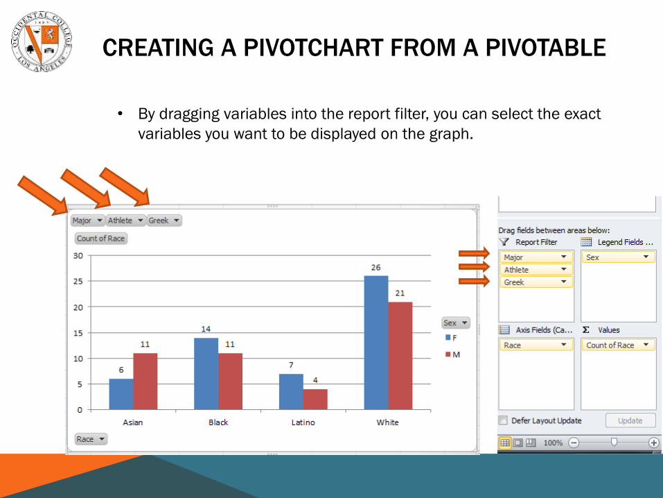
CREATING A PIVOTCHART FROM A PIVOTABLE
• By dragging variables into the report filter, you can select the exact
variables you want to be displayed on the graph.

CREATING A VLOOKUP FUNCTION
• Vlookup can retrieve data from other tables and
display it on your table of interest.
• The data in “Tabl2” is on an independent
spreadsheet
• Vlookup will allow us to display whether or not a
student is a 1st gen on our primary table
Note: make sure to
name your
secondary table.
This makes it easier
to create the vlookup
syntax
Table name
CREATING A VLOOKUP FUNCTION
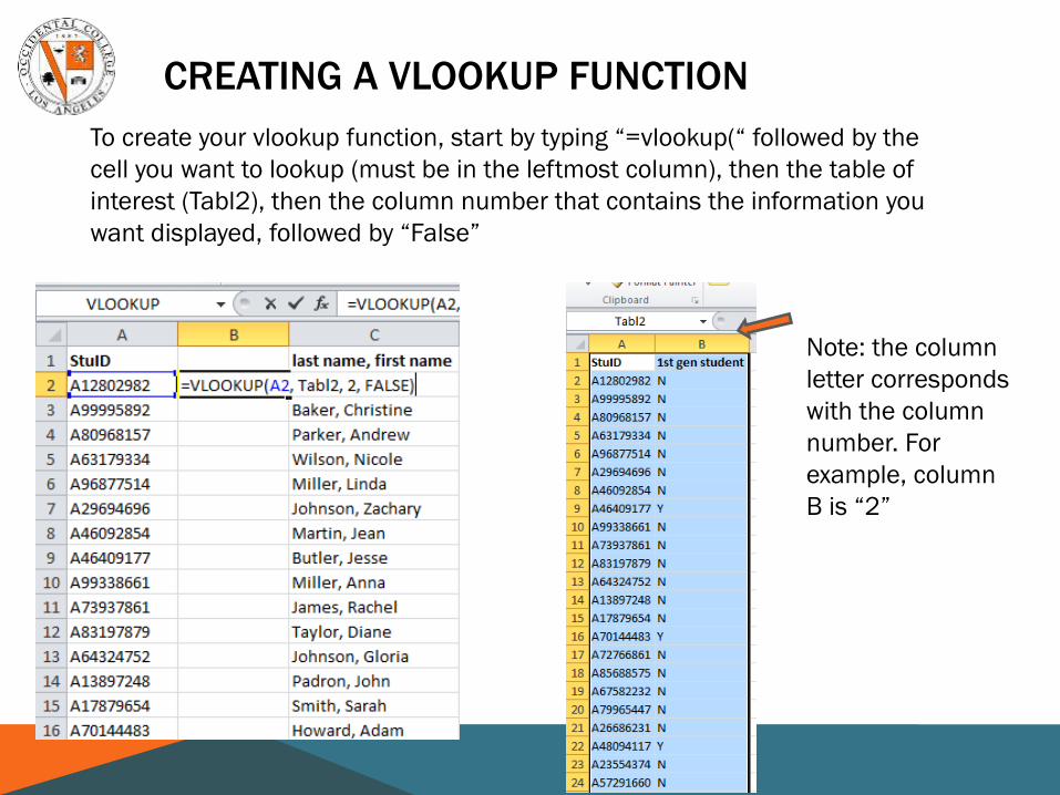
To create your vlookup function, start by typing “=vlookup(“ followed by the
cell you want to lookup (must be in the leftmost column), then the table of
interest (Tabl2), then the column number that contains the information you
want displayed, followed by “False”
Note: the column
letter corresponds
with the column
number. For
example, column
B is “2”

PRINT AREA
• To set your print area, select the data you want printed,
then go to Page LayoutPrint AreaSet Print Area


