
Who is Afraid of Black Scholes
A Gentle Introduction to Quantitative FinanceDay 2
July 12th 13th and 15th 2013UNIVERSIDAD NACIONAL MAYOR DE SAN MARCOS

Ito Calculus
• Suppose the stock price evolved as
• Problem with this model is that the price can become negative
Ito Calculus
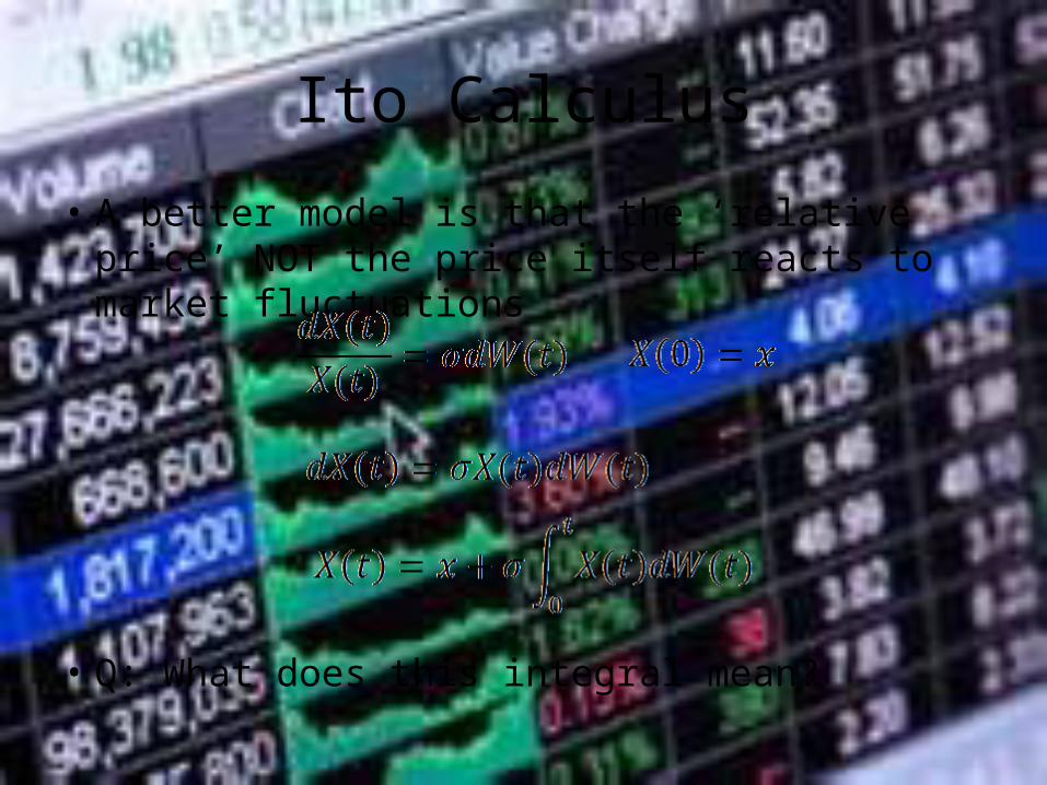
• A better model is that the ‘relative price’ NOT the price itself reacts to market fluctuations
• Q: What does this integral mean?

Constructing the Ito Integral
• We will try and construct the Ito Stochastic Integral in analogy with the Riemann-Stieltjes integral
• Note the function evaluation at the left end point!!!
• Q: In what sense does it converge?

Stochastic Differential Equations
• Consider the following Ito Integral
• We use the shorthand notation to write this as
• This is a simple example of a stochastic differential equation

Convergence of the Integral
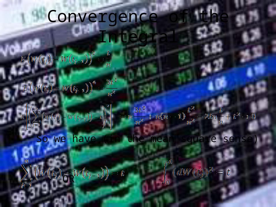
• We have noted the integral converges in the ‘mean square sense’
• To see what this means consider
• This means
Convergence of the Integral
So we have (in the mean square sense) OR

How to Integrate?• A detour into the world of Ito differential calculus
• Q: What is the differential of a function of a stochastic variable?• e.g. If what is • Is it true that in the stochastic world as well?• We will see the answer is in the negative• We will construct the correct Taylor Rule for functions of
stochastic variables• This will help us integrating such functions as well

Taylor Series & Ito’s Lemma• Consider the Taylor expansion
• The change in F is given by
• We note that behaves like a determinist quantity that is it’s expected value as
• i.e. formally!!

Taylor Series & Ito’s Lemma
• We consider when
• So the change involves a deterministic part and a stochastic part

Ito’s Lemma
• We consider a function of a Weiner Process and consider a change in both W and t
Ito’s Lemma

Ito’s Lemma
• Obtain an SDE for the process• We observe that
• So by Ito’s Lemma

Integration
• Using Ito we can derive
• E.g. Show that

Example • Evaluate
• Evaluate

Extension of Ito’s Lemma
• Consider a function of a process that itself depends on a Weiner process
• What is the jump in V if ?

Extension of Ito
• So we have the result
Example
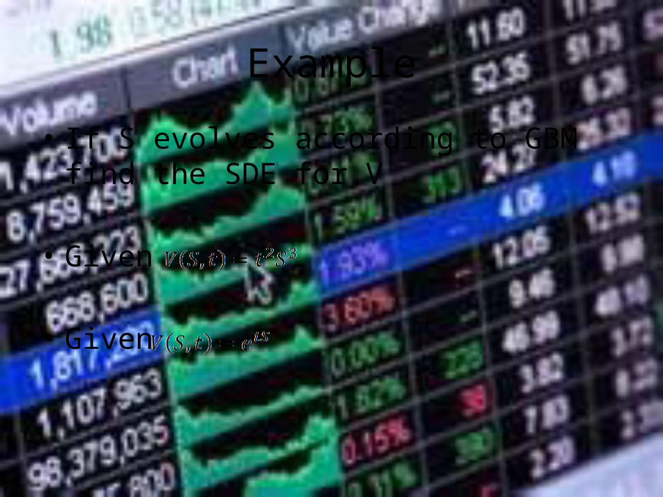
• If S evolves according to GBM find the SDE for V
• Given
• Given
Stochastic Differential Equation
• We will now ‘solve’ some SDE
• Most SDE do NOT have a closed form solution
• We will consider some popular ones that do

Arithmetic Brownian Motion
• Consider dX=aXdt+bdW• To ‘solve’ this we consider the process
• From extended Ito’s Lemma
Ito Isometry
• A shorthand rule when taking averages
• Lets find the conditional mean and variance of ABM

Mean and Variance of ABM
• We have using Ito Isometry

Geometric Brownian Motion
• The process is given by
• To solve this SDE we consider
• Using extended form of Ito we have

Black Scholes World• The value of an option depends on the price of the
underlying and time
• It also depends on the strike price and the time to expiry
• The option price further depends on the parameters of the asset price such as drift and volatility and the risk free rate of interest
• To summarize

Assumptions
• The underlying follows a log normal process (GBM)
• The risk free rate is known (it could be time dependent)
• Volatility and drift are known constants• There are no dividends• Delta hedging is done continuously• No transaction costs• There are no arbitrage opportunities

A Simple One Step Discrete Case

The Payoff

Short Selling

Hedging with the Right Amount

And the value is…….

Drift and Volatility

Delta Hedging
• How did one know the quantity of stock to short sell?
• Let’s re do the example:– Start with one option – And short on the stock
• The portfolio at the next time is worth– if the stock rises – if the stock falls

Delta Hedging
• We want these to give the same value
• In general we should go

The Stock Price Model
• Is out stock price model correct?

Derivation of Black Scholes Equation
• We assumed that the asset price follows
• Construct a portfolio with a long position in the option and a short position in some quantity of the underlying
• • The value of this portfolio is

Derivation
• Q: How does the value of the portfolio change?
• Two factors: change in underlying and change in option value
• We hold delta fixed during this step

Derivation
• We use Ito’s lemma to find the change in the value of the portfolio
• The change in the option price is
• Hence

Derivation
• Plugging in
• Collecting like terms

Derivation• We see two type of movements, deterministic i.e.
those terms with dt and random i.e. those terms with dW
• Q: Is there a way to do away with the risk?
• A: Yes, choose in the right way
• Reducing risk is hedging, this is an example of delta-hedging

Derivation
• We pick
• Now the change in portfolio value is riskless and is given by

Derivation
• If we have a completely risk free change in we must be able to replicate it by investing the same amount in a risk free asset
• Equating the two we get

Black Scholes Equation
• We know what should be
• This gives us the Black Scholes Equation

Black Scholes Equation
• This is a linear parabolic PDE
• Note that this does not contain the drift of the underlying
• This is because we have exploited the perfect correlation between movements in the underlying and those in the option price.

Black Scholes Equation
• The different kinds of options valued by BS are specified by the Initial (Final) and Boundary Conditions
• For example for a European Call we have
• We will discuss BC’s later

Variations: Dividend Paying Stock• If the underlying pays dividends the BS can be
modified easily• We assume that the dividend is paid
continuously • i.e. we receive in time • Going back to the change in the value of the
portfolio
Variations: Dividend Paying Stock
• The last terms represents the amount of dividend
• Using the same delta hedging and replication argument as before we have

Variations: Currency Options
• These can be handled as in the previous case
• Let be the rate of interest received on the foreign currency, then

Variations: Options on Commodities
• Here the cost of carry must be adjusted
• To simplify matters we calculate the cost of carrying a commodity in terms of the value of the commodity itself
• Let q be the fraction that goes toward the cost of carry, then
Solving the Black Scholes Equation• We need to solve a BS PDE with Final Conditions
• We will convert it to a ‘Diffusion Equation IVP’ by suitable change of variables
• Method of solution depends upon the PDE and BC
• Considering the BC in this case we will use the Fourier Transform Methods to find a function that satisfies the PDE and the BC
• Using different IC/FC will give the value for different options

Transforming the BS Equation
• Consider the Black Scholes Equation given by
• As a first step towards solving this we will transform it into a IVP for a Diffusion Equation on the real line

Transforming the BS Equation
• We make the change of variables
• This transforms the equation into
• Where

Transforming the BS Equation
• Choosing
• Letting
• Choose to simplify the expression

Transforming the BS Equation
• i.e. we take
• We get the following IVP

Introducing the Fourier Transform
• Our introduction will be very formal
• We will study only those properties that are needed to solve the IBVP
• We will derive a solution called the fundamental solution (Green’s function)
• This will allow us to find option pricing using BS

Fourier Transform
• We define the Fourier transform of ‘nice’ functions as
• The inverse transform is defined as

Fourier Transform: Properties
• We state some basic properties
– Linearity : If and then for
– Translation: for
– Modulation: If

Fourier Transform: Properties
• A very useful property for solving linear constant coefficients differential equations is
• Pf: Integrate by parts in the definition

Fourier Transforms Table of some common transforms
F(x) F(k)

Solving an IBVP
• We will use the Fourier Transform Method to solve the heat equation on an infinite domain
• PDE
• IC
• BC as

Solving the Heat Equation
• Take the Fourier Transform of both sides and assuming
• We have using the properties of FT
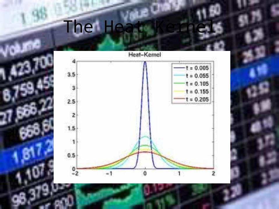
The Heat Kernel
Solving the Heat Equation
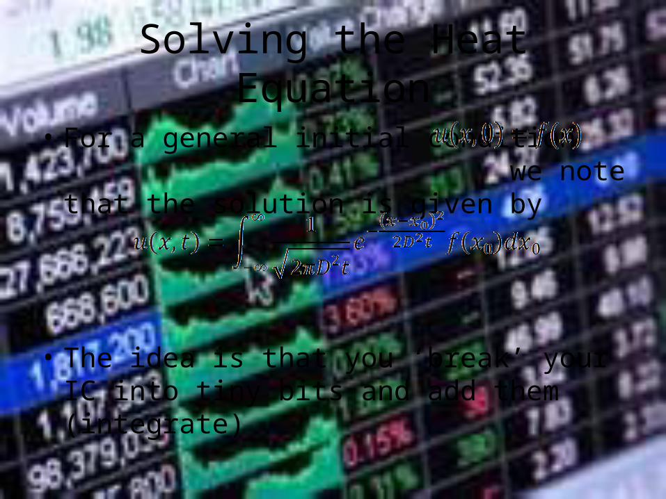
• For a general initial condition we note that the solution is given by
• The idea is that you ‘break’ your IC into tiny bits and add them (integrate)

Back to the Black Scholes Equation
• We had transformed the B-S FVP to the IVP
• Where

Solving the Black Scholes for a European Call
• Here the final condition is replaced by the IC
• Recalling the IVP and the fundamental solution, we have

Solving the Black Scholes for a European Call
• Going back to the original variables
• The call option has the payoff

Solving the Black Scholes for a European Call
• Substituting into the solution we have
Solving the Black Scholes for a European Call
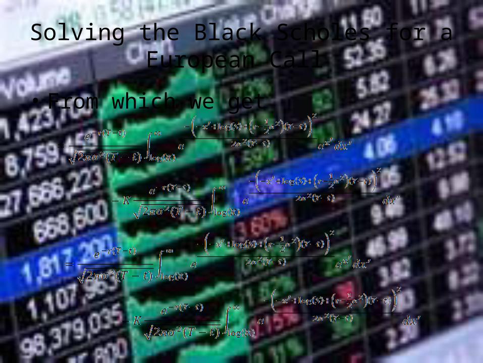
• From which we get
Solving the Black Scholes for a European Call
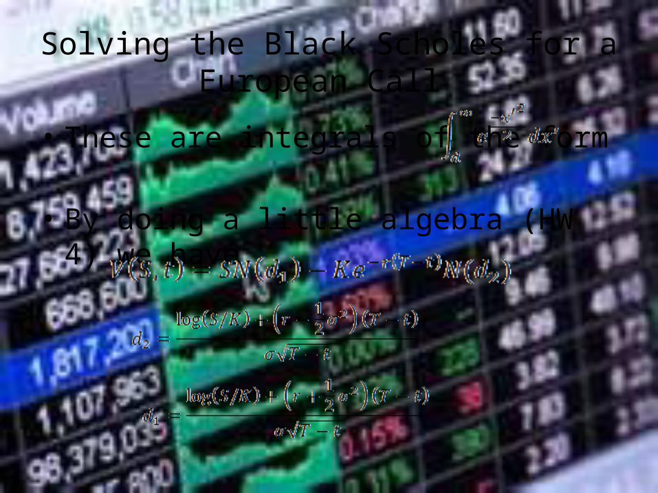
• These are integrals of the form
• By doing a little algebra (HW 4) we have

European Call Option

The Black Scholes PDE
• Consider the Black Scholes Equation given by
• European Call• European Put• Binary Options• American Style Options

Solution of Black Scholes for a European Call
• Solution for a European Call

Solution for a European Put• We use the put call parity
• Using the solution for a European Call
• Noting
• We have
Calculating the Greeks
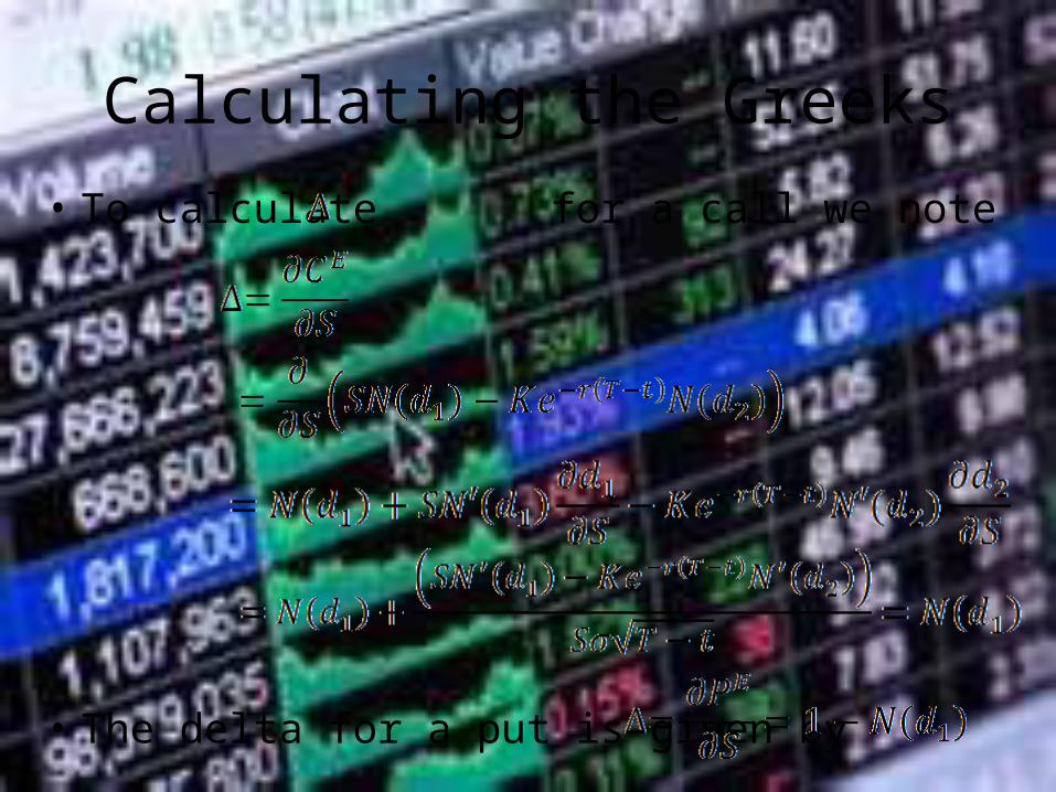
• To calculate for a call we note
• The delta for a put is given by
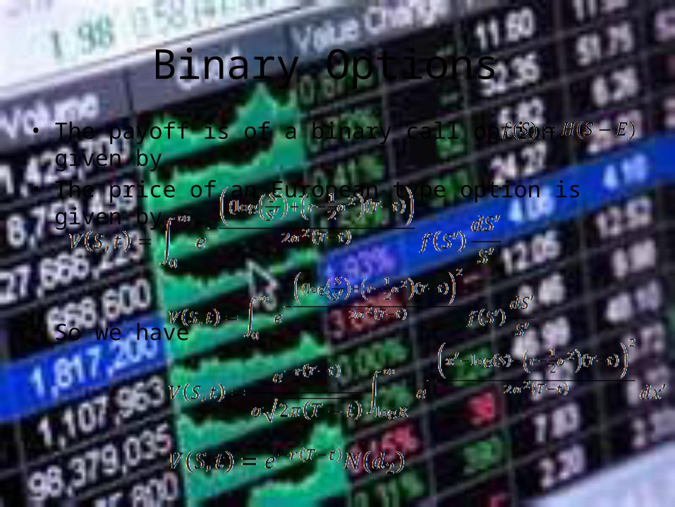
Binary Options • The payoff is of a binary call option given by• The price of an European type option is given by
• So we have
American Options
• These can be exercised anytime prior to and at expiry
• Issue with analyzing these is ascertaining when to exercise
• This will lead to a free boundary problem

American Options
• Note that if the previous was the value of an American Put then there would be an arbitrage opportunity. i.e. If an arbitrage opportunity exists
• Pf: Buy the assent in the market for S and the option for P, immediately selling the asset for K by exercising the option. We make a risk free profit of
• Hence for the American Option we have

Perpetual American Put
• This can be exercised at any point and there is not expiry
• The payoff is
• We have already note that
• The option must satisfy the BS ODE
Perpetual American Put
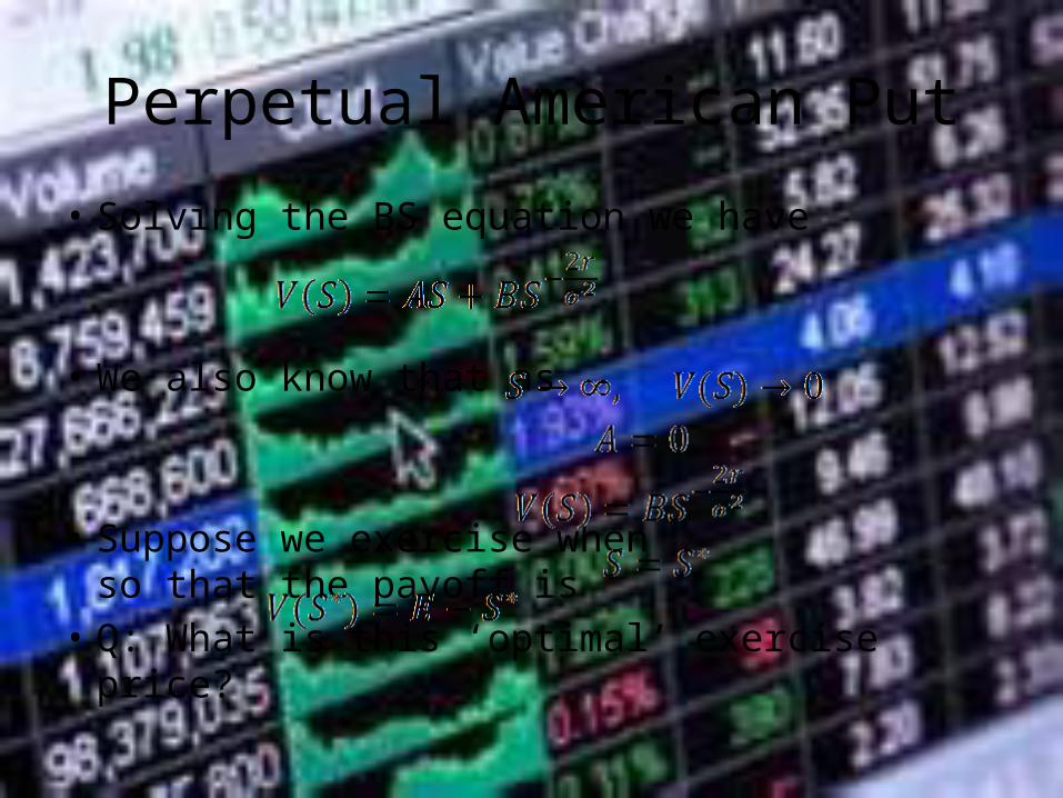
• Solving the BS equation we have
• We also know that as
• Suppose we exercise when so that the payoff is
• Q: What is this ‘optimal’ exercise price?

Perpetual American Put
• This gives us the value of B
• Q: What maximizes V?• Setting

Perpetual American Put
• Notice the slope of the payoff function and the option value are the same at
• This is called the smooth pasting condition

Perpetual American Options with Dividends
• Let’s consider the perpetual American Call with dividends
• This has solutions
• The perpetual put now has value
• It is optimal to exercise when
Perpetual American Call with Dividends
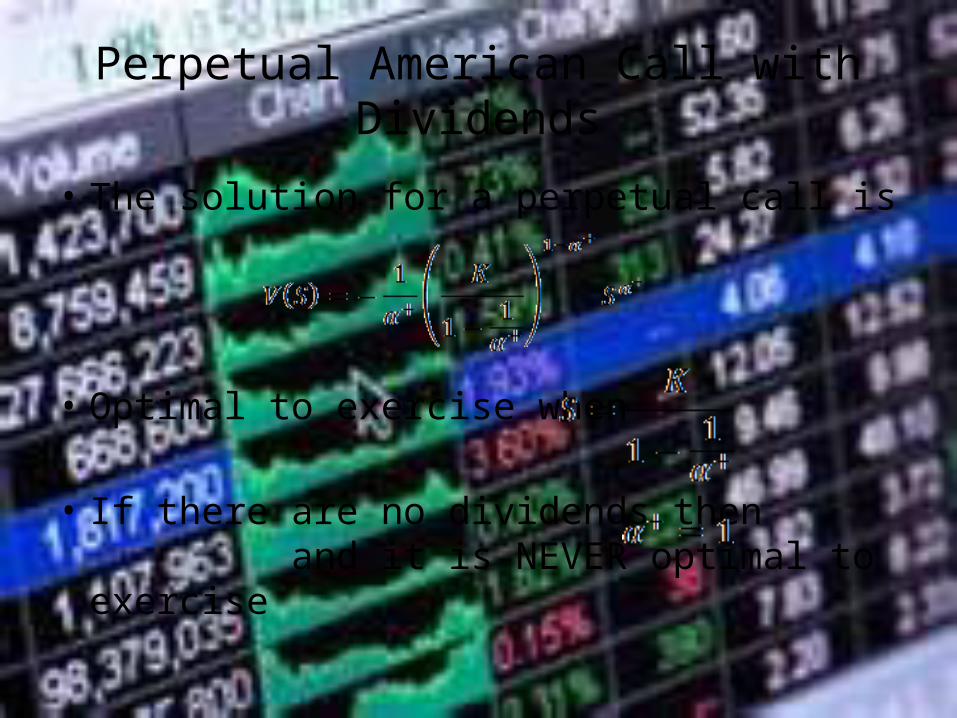
• The solution for a perpetual call is
• Optimal to exercise when
• If there are no dividends then and it is NEVER optimal to exercise
American Options with Finite Time Horizon
• Consider the case where the strike time is finite
• We construct a portfolio with one option and short Δ of the underlying
• Change in the value of the portfolio in access of the risk free rate is

American Options with Finite Time Horizon
• We delta hedge to obtain
• We have three possibilities

American Options with Finite Time Horizon
• We consider them each• – There is an arbitrage opportunity as one can buy the
option and short sell the asset and loaning out the cash• – There is an arbitrage opportunity as one can sell the
option and buy the asset borrowing cash • In the American Option case the second strategy
will not always lead to arbitrage as exercising the option in no longer in the hands of the seller

American Options with Finite Time Horizon
• So we have
(Payoff for early exercise)
is continuous

American Options with Finite Time Horizon
• Q: How to go about ‘solving’ this?
• A: Closed form solutions not available Will sue numerics (finite difference) Recast as a Linear Complementarity
problem


