
JOURNAL OF REGIONAL SCIENCE, VOL. 54, NO. 5, 2014, pp. 755–787
WHY DO RENTERS STAY IN OR LEAVE CERTAIN NEIGHBORHOODS?THE ROLE OF NEIGHBORHOOD CHARACTERISTICS, HOUSINGTENURE TRANSITIONS, AND RACE*
Kwan Ok LeeDepartment of Real Estate, National University of Singapore, 4 Architecture Drive, SDE1-03-03,Singapore 117566, Singapore. E-mail: [email protected]
ABSTRACT. Given significant variation in population turnover and stability across neighborhoods,this study examines why renters stay in or leave certain neighborhoods. It is the first to analyzehow neighborhood characteristics influence renters’ decisions to move within the neighborhood aswell as how these decisions are interrelated with their housing tenure transitions and race. Resultsdemonstrate that homeownership rates have a significant, positive association with the probabilitythat renters stay and/or purchase homes in the current neighborhood. Both the tenure compositionof the housing stock and higher neighborhood satisfaction appear to be central in understanding thisassociation. Results also suggest that nonblack renters are more likely to leave neighborhoods thatexperience growth in the percentage of the black population, while blacks are more likely to stay andpurchase homes within such neighborhoods.
1. INTRODUCTION
About half of all households in the United States move every five years and one-third of the renter households move every year (Briggs, 2005). According to the 2000Census, 15.5 percent of households moved to their current residence within a year. This ismuch higher than 5 percent of annual residential mobility in Europe (David, Janiak, andWasmer, 2008) and 5 percent in Japan (Seko and Sumita, 2007) for a similar time period.The 2000 Census further indicates that American households are more likely to stay incertain neighborhoods than in others. As Figure 1 depicts, the share of households thathave moved to their current residence within five years significantly differs across censustracts within the same county. While only 24 percent of residents are recent migrantsin certain census tracts of Los Angeles County, more than 90 percent of residents havestayed shorter than five years in other tracts within the same county.
Understanding why households stay in or leave certain neighborhoods is importantbecause these decisions have a substantial impact on the surrounding neighborhoodand the welfare of household members, especially children. There are potential externalcosts associated with neighborhood instability and a lack of social cohesion in rapidlytransitioning neighborhoods with higher population turnover. Shaw and McKay (1969)and Sampson, Raudenbush, and Earls (1997) suggest evidence that these neighborhoodsmay suffer from neighborhood problems, including violence and other criminal activities.Children in households that frequently move between different neighborhoods are likelyto experience school instability (Simmons et al., 1987; Coleman, 1988, 1990; Hagan,MacMillan, and Wheaton, 1996).
*The author thanks anonymous reviewers, Marlon Boarnet, Gary Painter, Jenny Schuetz, and GeorgeGalster for support, comments, and useful advice.
Received: July 2012; revised: February 2014; accepted: March 2014.
C© 2014 Wiley Periodicals, Inc. DOI: 10.1111/jors.12124
755

756 JOURNAL OF REGIONAL SCIENCE, VOL. 54, NO. 5, 2014
Source: Author’s own analysis of the Censes 2000.Notes: The figure shows the share of households who moved to the current residence after 1995.
FIGURE 1: Population Mobility Rates in Los Angeles County.
To explain residential mobility, previous research focused on household-specific de-terminants, including race and income, life-cycle covariates such as age and a changein family composition, a job change, and the characteristics of the current dwelling (forreviews, see Clark and Dieleman, 1996; Dieleman, 2001). More recently, the literaturehas started to consider moving as an outcome of dissatisfaction with the neighborhoodenvironment and analyze cross-neighborhood variation in population turnover. Severalneighborhood characteristics are known to matter for residential mobility, including theshare of owner-occupied and single-family units (Bailey and Livingston, 2007; van Hamand Clark, 2009), relative economic status (Harris, 1999; Quillian, 1999, 2003; Feijtenand van Ham, 2009), and racial composition (Taub, Taylor, and Dunham, 1984; Harris,1999; Crowder, 2000; Ellen, 2000).
The primary contribution of this study is to focus on the diverse underlying mecha-nisms through which neighborhood characteristics—including homeownership rates, eco-nomic gentrification (i.e., increase in the ratio of tract-to-area median household income),and change in racial composition—influence residential mobility of renter households.To the author’s current knowledge, this is the first analysis that estimates a full rangeof residential mobility choices, including a no-move as well as inter- and intraneighbor-hood moves. As Figure 2 demonstrates, about 37 percent of local moves of Panel Studyof Income Dynamics (PSID) renter households take place within the census tract of cur-rent residence. This analysis reports how neighborhood characteristics are associatedwith these intraneighborhood moves that would significantly reduce neighborhood popu-lation turnover. This study is further able to investigate the dynamic interplays betweenneighborhood characteristics and residential mobility among individual renters underdifferent circumstances. For instance, the association between change in the stock ofowner-occupied units and moving decisions may differ for continuing renters and home-buyers that make a transition from renting to owning. However, neighborhood satisfaction
C© 2014 Wiley Periodicals, Inc.

LEE: WHY DO RENTERS STAY IN OR LEAVE CERTAIN NEIGHBORHOODS? 757
Source: Author’s own analysis of the Panel Study of Income Dynamics.
FIGURE 2: Joint Choices of Residential Mobility and Housing Tenure Transition.
that tends to be higher in neighborhoods with higher homeownership rates would matterfor moving decisions regardless of housing tenure transitions. Renters’ responsiveness tochange in the racial composition of surrounding neighbors may also vary with their ownrace.
In analyzing these dynamics, this study estimates models that jointly consider thedecision of residential mobility and housing tenure transition as well as models stratifiedby household race. It also raises the potential selection bias concerns and employs anempirical approach that controls for time-invariant, unobserved heterogeneity of samplerenters. This study uses a unique dataset that matches longitudinal household data fromthe geocoded PSID to census tract-level data from the U.S. Census. These data enablethe research to identify the census tract where the household resides in a given yearand to append neighborhood characteristics (i.e., the share of owner-occupied units, theratio of tract-to-area median household income, and the share of blacks) as well as annualchanges in them. In addition, the data allow controlling for the financial and demographiccharacteristics of renters that are known to be important for their moving decisions.
The results based on various modeling approaches consistently demonstrate thathomeownership rates have a significant, positive association with the probability thatrenter households stay and/or purchase homes in the current neighborhood. Renterswould not only find greater homeownership opportunities within this neighborhood butalso be more satisfied with the neighborhood since homeownership rates can be a proxyfor higher neighborhood quality and homeowners can generate positive externalities (e.g.,neighborhood social capital). The estimation results also suggest that nonblack rentersare more likely to leave the neighborhood that experiences growth in the percentage ofthe black population, while black renters are more likely to stay and purchase homeswithin such neighborhood. Results regarding economic gentrification are not consistent.The simulations suggest that the probability that white renters leave the neighborhoodis 5.8 percentage points higher if the share of the black population in their neighborhoodis one standard deviation higher. For a comparison, being out of the married state is
C© 2014 Wiley Periodicals, Inc.

758 JOURNAL OF REGIONAL SCIENCE, VOL. 54, NO. 5, 2014
associated with about a 5.8 percentage point increase in the probability of leaving theneighborhood.
2. BACKGROUND
Households are likely to consider moving within metropolitan areas (MSAs) or coun-ties, defined as intraurban migration or residential mobility, when they are not satisfiedwith current housing attributes and/or neighborhood environment (Quigley and Weinberg,1977). Building on Speare, Goldstein, and Frey (1975), earlier empirical models of resi-dential mobility put an emphasis on household-specific determinants, including race andincome, life-cycle covariates such as age and a change in family composition, a job change,and the characteristics of the current dwelling (for the review, see Clark and Dieleman,1996; Dieleman, 2001). More recent research has discussed how current neighborhoodsinfluence the desires and decisions to relocate elsewhere (Galster, 1987; Lee, Oropresa,and Kanan, 1994). Among neighborhood characteristics that are known to be associatedwith residential mobility, the discussion in this section focuses on homeownership rates,economic gentrification, and change in racial composition.
Homeownership Rates
It is well known that higher homeownership rates are associated with lower popula-tion turnover at the neighborhood level (e.g., Lee, Oropresa, and Kanan, 1994; Dieleman,Clark, and Deurloo, 2000). Since empirical analyses at the disaggregate level have beenquite rare, however, the current evidence is inconclusive concerning the mechanism bywhich homeownership rates influence the moving choices of individual households, espe-cially renter households. There are three potential mechanisms. First, households may bemore satisfied with the neighborhoods with higher homeownership rates. Homeownershave likely chosen higher quality neighborhoods because they generally have higher finan-cial capacity and take greater care in choosing neighborhoods than renters (Haurin, Di-etz, and Weinberg, 2005). Therefore, homeownership rates could be a proxy of unobservedneighborhood quality. Furthermore, homeowners tend to contribute to neighborhood sta-bility and the maintenance of the surrounding environment (Rohe and Steward, 1996) aswell as generate higher social capital through interactions among neighbors (Rosenthal,2008). Therefore, neighborhood satisfaction among households would be higher in neigh-borhoods with a concentration of homeowners and one could expect higher homeownershiprates to reduce the probability that renters leave the neighborhood.
Second, homeownership rates determine the stock of owner-occupied units relativeto rental units within the neighborhood influencing continuing renters and homebuy-ers in a different way. On the one hand, this “stock effect” may involve the conversionof rental units to owner-occupied units and leave fewer rental housing options in theneighborhood. Thus, renters wanting to continue to rent may choose to leave the neigh-borhood. On the other hand, homeownership rates indicate home-buying opportunitieswithin the neighborhood where the renter household currently resides. This would mat-ter to renters seeking a home to buy within their current neighborhood. Dawkins (2005)and Kan (2007) list several reasons for this searching behavior, including travel costsfor searching, proximity between the current neighborhood and work places, more in-formation about local housing markets, and existing local social network. If potentialhomebuyers are able to purchase homes that they desire within the current neigh-borhood, they would therefore move within the neighborhood. Otherwise, householdswould remain renters in the current neighborhood or purchase homes in an alternativeneighborhood.
C© 2014 Wiley Periodicals, Inc.

LEE: WHY DO RENTERS STAY IN OR LEAVE CERTAIN NEIGHBORHOODS? 759
Finally, the homeowning interest of an individual renter may be influenced by hisneighbor’s interest in homeowning (Manski, 1993; Ioannides and Zabel, 2003). If this“peer effect” exists, homeownership rates would influence the probability that rentersbecome homeowners, and, in turn, affect their decision whether to stay in or leave theneighborhood since housing tenure transitions are endogenous to residential mobilitydecisions. This study employs the empirical framework accounting for such endogeneity,as suggested by recent research on housing tenure choice (Deng, Ross, and Wachter, 2003;Gabriel and Painter, 2008).
Economic Gentrification
There is evidence that households tend to move away from poor neighborhoods asbest as their financial capacity allows them to do so (Harris, 1999; Quillian, 1999, 2003).Parkes and Kearns (2003) also find that householders living in economically decliningneighborhoods are more likely to think about moving out but less likely to do so dueto lack of financial capacity. However, the current evidence is mixed on whether theincrease in a neighborhood’s economic status would impact residential mobility. Hartman(1979) and Smith (1996) hypothesized that economic gentrification may contribute toescalating rents and, in turn, displace renter households from the neighborhood. Morerecent research (Vigdor, Massey, and Rivlin, 2002; Freeman and Braconi, 2004; Freeman,2005; McKinnish, Walsh, and White, 2010), however, suggests that such displacementmay not be widespread. Ellen and O’Regan (2011) also provide evidence that economicgentrification can lead to higher satisfaction of existing residents because of improvedneighborhood quality. By this reasoning, it is expected that controlling for the changein housing costs, an increase in neighborhood income would decrease the probabilityof renters moving out of the neighborhood. However, the literature does not provideguidance as to whether economic gentrification can play a different role for homebuyersand continuing renters. While an increase in rents would be more burdensome to somecontinuing renters, gentrification may be able to relieve the increase in housing costs andcontribute to home-buying activities to the extent that housing units are renovated ornewly constructed in the gentrifying neighborhoods.
Change in Racial Composition
The literature suggests two mechanisms by which change in racial composition couldinfluence residential mobility. First, Schelling (1969) hypothesizes that preferences forracial composition of surrounding neighbors differ between blacks and whites so thattheir residential mobility can be influenced by a change in racial composition. Empiricalstudies provide evidence of white flight from neighborhoods where minority shares signif-icantly increase (Crowder, 2000; van Ham and Clark, 2009). In particular, when minorityshares exceed the “tipping point,” the neighborhood is likely to transition into a pre-dominantly minority neighborhood (Card, Mas, and Rothstein, 2008). Second, the “racialproxy hypothesis” suggests that the population of minority residents is closely associatedwith a whole range of neighborhood problems (Taub, Taylor, and Dunham, 1984; Clark,1992; Harris, 1999) and households tend to perceive an increase in minority residentsin the neighborhood as a sign of neighborhood decline (Ellen, 2000). Hence, we can positthat both minority and nonminority households may move out of a neighborhood that isbecoming minority-concentrated not because of their preferences per se but because ofperceived effects. In addition, as indicated by Harris (1999) and Crowder (2000), it wouldbe critical to control for other neighborhood characteristics so that the effect of the racialcomposition is not to be a simple proxy for the effect of these characteristics.
C© 2014 Wiley Periodicals, Inc.

760 JOURNAL OF REGIONAL SCIENCE, VOL. 54, NO. 5, 2014
3. DATA AND METHODS
Data
As collected by the Survey Research Center at the University of Michigan, the PSIDis a longitudinal dataset beginning in 1968 with approximately 4,800 families and pro-vides detailed demographic, economic, and housing information for each family. The PSIDis ideally suited for examining the interaction of neighborhood factors with the likelihoodthat households stay in the neighborhood. First, it has good information on housing statusincluding tenure, structure, and the number of rooms. Second, the PSID contains excellenthousehold-specific control variables, including respondents’ economic status and demo-graphics. Finally, the longitudinal nature of the PSID offers many benefits to capturedemographic and economic transitions such as a divorce, the birth of a child, and unem-ployment. As suggested by previous literature, these transitions could be a trigger eventfor residential mobility and housing tenure.
The PSID Geocode Match Files allow for the merging of the PSID with the Censusthrough census tract identifiers.1,2 Hence, this study can measure a change in residentiallocation of each household between two survey years as well as append neighborhoodfactors at the census tract level. The unit of analysis is a household and a sample is limitedto renter householders over the years 1972–2003. Households are included in the sampleif they are renters at least in one year during the observation period and appear withvalid geocodes for two or more successive survey years so that their residential mobilitycan be identified between these years. Then, these households are followed until theymake a tenure transition to homeownership or until they are completely dropped fromthe PSID sample.3 There are 10,420 households that meet the above criteria. Each yearin which a household is observed constitutes a household-year and most households inthe sample contribute information about several household-years. The average numberof years observed for one renter household is about 7.5 years and the total number ofhousehold-years is 78,028. Among them, 55,294 household-years have valid informationfor all variables used for the analysis.4
This study defines a neighborhood as the census tract, following most prior research(e.g., Massey, Gross, Shibuya, 1994; Quillian, 2002; Crowder and South, 2008; Ellen andO’Regan, 2011). It also defines residential mobility to include both intraneighborhoodmoves (a change of the unit within the same tract) and interneighborhood moves (a changeof the census tract within the same MSA or county). It limits residential mobility to
1While the PSID publicly provides longitudinal household data, geocode match files are released onlyunder the special contract.
2Because many variables at the census tract level are not available in the 2010 Census (i.e., LongForm or Summary File 3), the analysis instead uses the 2005–2009 American Community Survey (ACS)five-year estimates to annually interpolate data for 2001 and 2003.
3One may be concerned with a sample attrition issue. On average, 7.7 percent of households havebeen dropped out of the sample per year, which is not a considerable proportion. The literature (e.g.,Fitzgerald, Gottschalk, and R. Moffitt, 1998) also reports no strong evidence that attrition has seriouslydistorted the representativeness of the PSID. Still, the additional analysis was done with the sampleexcluding the households who have been dropped out. The results remain consistent. Finally, this analysisemploys PSID weights that address potential statistical issues of sample attrition to some extent.
4As shown in Figure 2, about 8 percent of household-years are dropped because they are long-distancemoves. About 15 percent of the remainder does not have the valid geocodes (tract, county, or MSA codes)to be merged with the Census data from two adjacent census years. There are more losses of observationsfor the period of 1986–1990 because the 1980–1990 Census Tract Relationship File is used for this periodwhere the 1980 census tract codes are not available (see Footnote 7). Another 7 percent do not have validinformation for other household-level variables.
C© 2014 Wiley Periodicals, Inc.

LEE: WHY DO RENTERS STAY IN OR LEAVE CERTAIN NEIGHBORHOODS? 761
short-distance moves because moves across MSAs and counties are more likely to betriggered by nonresidential reasons such as job changes that may be less related withneighborhood factors. A renter household who moves from one to another MSA would beout of the sample for this particular year but reenters the sample once it lands in a newMSA and if it still remains a renter. The PSID Geocode Match Files contain residentiallocation of each household for each survey year using the census tract boundary definitionin 1970, 1980, 1990, and 2000. To consistently trace residential mobility over the sampleperiod, the 2000 tract boundary definition is used to measure residential locations ofhouseholds across years.
The key independent variables in the analysis are a set of static neighborhood char-acteristics and neighborhood change. Main neighborhood variables include the homeown-ership rate, the ratio of tract-to-area median household income, and the share of the blackpopulation.5 Also, an interaction between household’s race and the share of the black pop-ulation is added. All these neighborhood variables are obtained at the census tract levelfrom the decennial Census and linear interpolation is used to fill in values for noncensusyears.6 To deal with the change of census tract boundaries between census years, thisstudy uses a method called “place-to-place interpolation” suggested by Quillian (1999:16).7,8 Static neighborhood characteristics are measured for the census tract of residencein year t – 1 to observe how they are associated with residential mobility in a current yeart. Using the lagged variables could help reduce potential endogeneity between neigh-borhood characteristics and residential mobility of individual households. Since the datacontain annual neighborhood data even for noncensus years by using linear interpolation,neighborhood change between the years can be imputed as well. It is calculated as thevalue in year t – 1 minus the value in year t – 2 in the current neighborhood prior to aresidential mobility decision in year t. Renters are likely to observe changes within theircurrent neighborhood as well as across the neighborhoods within the same MSA and make
5For additional specifications in the later part of this paper, the ratio of tract-to-area median rent isalso used.
6Using the annually interpolated data allows accounting for neighborhood change over time. Thiswould not be a problem for neighborhood characteristics that are likely to change slowly between censusyears, including the share of owner-occupied units, the share of older units, and the share of black popula-tion. Other neighborhood factors such as neighborhood housing price or neighborhood income status mayhave larger annual variation. Since this analysis uses a relative measure for them (tract-to-area ratio),however, the size of their changes between census years is quite small (e.g., mean of tract-to-area neigh-borhood income for all years: 88.6 percent; average change in tract-to-area neighborhood income betweencensus years: 3.5 percent).
7This method takes advantage of this geocoded PSID, which provides census tract codes of differentcensus years for the residence of PSID respondents. Since we know the census tract of the residence iscoded X in the 1990 census and it is coded Y in the 2000 census, neighborhood variables can be linearlyinterpolated between these census years. In fact, in creating their Geocode Match Files, the PSID doesattempt to match all tract boundaries from the two censuses, while some tracts undergoing the drasticboundary changes are left unmatched (Adams, 1991). If X and Y have the different tract boundaries andthese boundaries can represent a real concept of neighborhoods, using this method would be beneficialbecause it can account for a change in neighborhood boundaries. If tract boundaries change in a morearbitrary way, neighborhood change observed by using this method would simply reflect an arbitrarychange in tract boundaries rather than actual change in neighborhood boundaries. While the geocodedPSID does not provide the 1980 Census tract codes for the period of 1986–1990, 1990 Census tract codesare available even for this period. Therefore, the 1980 tract-level data for 1986–1990 were obtained byusing the 1980–1990 Census Tract Relationship File.
8Several recent studies rely on using the Neighborhood Change Database (NCDB), constructed byGeoLytics in collaboration with the Urban Institute, to mitigate potential problems associated with tractboundary changes across censuses.
C© 2014 Wiley Periodicals, Inc.

762 JOURNAL OF REGIONAL SCIENCE, VOL. 54, NO. 5, 2014
residential mobility decisions, so households who have stayed in a given neighborhood forless than two years are excluded for the models with neighborhood change.
Finally, the analysis is controlled for traditional variables that have been utilized byresearchers modeling residential mobility. These control variables include: (1) household-level demographic characteristics that could predict residential preferences of householdsand their mobility propensities, such as age, race, and sex of household head, maritalstatus, number of children, and education of household head as well as demographictransitions that could reflect changes in residential needs, such as a marriage, a divorce,and the birth of a child in a given year; (2) household-level economic characteristics thatcould determine financial capacity to move, including employment status, permanentincome as calculated with a five-year moving average, and transitory income; (3) otherhousehold-level characteristics including homeownership experience potentially reflect-ing households’ tastes for homeownership, years residing in the current home describingpast mobility patterns,9 and the number of rooms per person and housing structure thatare related with current residential conditions; and (4) region and year dummies. Thecomplete list of variables used for the analysis is presented in Table A1.
Methodology
A main empirical model used for this study is a multinomial logit (MNL) model. In anMNL model,10 a dependent variable represents joint choices of residential mobility andhousing tenure transition. Residential mobility is divided into two categories: intraneigh-borhood (INTRANt), and interneighborhood (INTERNt). All households start as a renterand their binary choice of housing tenure transition (HTTt) is made on whether to becomea homeowner or to remain a renter.11 Therefore, there are five different choice outcomes(also see Figure 2), denoted by MTit, such that
MTit = 0 if household i does not move at all (INTRANt = 0, INTERNt = 0, HTTt = 0),MTit = 1 if household i moves within a neighborhood and remains a renter (INTRANt =
1, INTERNt = 0, HTTt = 0),MTit = 2 if household i moves within a neighborhood and becomes a homeowner (IN-
TRANt = 1, INTERNt = 0, HTTt = 1),MTit = 3 if household i moves out of a neighborhood and remains a renter (INTRANt = 0,
INTERNt = 1, HTTt = 0),MTit = 4 if household i moves out of a neighborhood and becomes a homeowner (IN-
TRANt = 0, INTERNt = 1, HTTt = 1).
9As an additional check, the quadratic term for the number of years in home was added to the modelsand the results regarding neighborhood characteristics and neighborhood change did not change.
10A simple closed-form structure of a MNL model makes it easy to estimate and interpret. However,several relevant studies caution that a MNL approach could impose the independence of irrelevant alter-natives (IIA) by restricting the error structure to be independent, identically distributed (IID) with type Iextreme value distribution and suggest methodologies to relax the IID assumption. For example, recogniz-ing the potential interdependence between choice outcomes of mobility and housing tenure, Ioannides andKan (1996) and Kan (2000) use a multinomial probit (MNP) approach for their joint models. While thisMNP approach could avoid the potential IIA violation, however, it relies on the functional form assump-tions. Alternatively, Gabriel and Painter (2008) use a nested MNL (NMNL) model. This could relax theIIA assumptions, but requires strong assumptions on the nesting structure among alternative residentiallocation and homeownership choices.
11Some households change tenure in place. These households are treated as moving within theneighborhood and becoming homeowners in this analysis.
C© 2014 Wiley Periodicals, Inc.

LEE: WHY DO RENTERS STAY IN OR LEAVE CERTAIN NEIGHBORHOODS? 763
Let (p0, p1, . . . , p4) be the probabilities of each alternative choice among the abovefive possible outcomes. The probability of the household i to choose the alternative j atthe time t is given by
pitj = Pr(MTit = j) = exp(Xit�1)/[∑
exp(Xit�1)], j = 0, 1, . . . , 4,(1)
where Xit is the vector of the independent variables associated with the household i atthe time t, representing the set of neighborhood factors at the time t − 112 and the setof household-specific demographic and economic attributes at the time t, and �j is thevector of parameters associated with the alternative j. Because MTit = 0 is the baseoutcome, coefficients of all independent variables associated with each alternative choiceare estimated with respect to this “No Move” category. Hence, the vector of coefficientsassociated with it, �0, is normalized to zero without loss of generality.
This MNL model pools 29 cross sections of local moves of renter households.13 Ac-cordingly, the data are structured in “household-year” format, with each observation per-taining to the PSID interview year. Since the same renter households could contributemore than one household-year to the analysis and both residential mobility and housingtenure transition are repeatable events (e.g., the household moves within the neighbor-hood and remain a renter between year t – 1 and t, and then leaves the neighborhoodand buys a home between year t and t + 1), the above model may violate the standardassumption that observations are the independent. This issue is handled by clusteringstandard errors at the household level. The standard errors clustered in this way appear,on average, about 2–2.5 times greater than those computed without clustering.
4. RESULTS
Descriptive Statistics
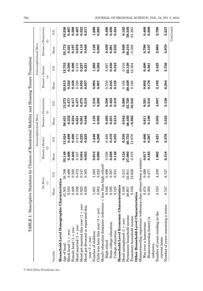
Figure 2 shows the flow of residential mobility and homeownership transition of thesample renter households in a given interview year. Between two consecutive interviewyears, about 53 percent of the sample households stay in the current house and about39 percent move only within the same MSA or county. This is consistent to Crowder andSouth (2008) using the geocoded PSID. Comparably, the 2000 Census shows that overthe period of five or more years, about 25 percent of renters have stayed in the samehouse and about 80 percent of all households have remained within the same MSA orcounty. While it is not surprising that most moves take place in the local context (Quigleyand Weinberg, 1977), what has been less known is whether these movers choose to movewithin the same neighborhood or move to another neighborhood within the MSA or county.According to Figure 2, about 36 percent of local moves take place within the same censustract of current residence. More than 23 percent of these intraneighborhood moves areaccompanied with the home purchases.
Table 1 displays variation in the attributes of sample renter households making dif-ferent residential mobility and housing tenure choices and indicates where the variationbetween the no-move choice group (column 1) and other choice groups (column 2–column
12As mentioned earlier, this analysis uses a lagged variable of neighborhood characteristics to avoidthe endogeneity issues (e.g., homeownership rates are endogenous to housing tenure transition of resi-dents).
13There are 29 waves for the main MNL model, including 1972–1996, 1997, 1999, 2001, and 2003.Note that the years of 1970–1971 are excluded since information associated with neighborhood change(i.e., the 1960 Census) is not available for these years and that the PSID has become biennial since 1997.
C© 2014 Wiley Periodicals, Inc.
764 JOURNAL OF REGIONAL SCIENCE, VOL. 54, NO. 5, 2014
TA
BL
E1:
Des
crip
tive
Sta
tist
ics
byC
hoi
ces
ofR
esid
enti
alM
obil
ity
and
Hou
sin
gT
enu
reT
ran
siti
on
Intr
anei
ghbo
rhoo
dM
ove
Inte
rnei
ghbo
rhoo
dM
ove
No
Mov
eR
emai
na
Ren
ter
Bec
ome
aH
omeo
wn
erR
emai
na
Ren
ter
Bec
ome
aH
omeo
wn
er(1
)(2
)(3
)(4
)(5
)
Var
iabl
eM
ean
S.D
.M
ean
S.D
.M
ean
S.D
.M
ean
S.D
.M
ean
S.D
.
Hou
seh
old
-Lev
elD
emog
rap
hic
Ch
arac
teri
stic
sA
geof
hea
d41
.501
16.7
0633
.148
13.5
2436
.451
13.2
7332
.615
12.7
5333
.773
10.3
36B
lack
hea
d(1
=ye
s)0.
533
0.49
90.
468
0.49
90.
332
0.47
10.
522
0.50
00.
321
0.46
7F
emal
eh
ead
(1=
yes)
0.48
80.
500
0.40
20.
490
0.22
40.
417
0.43
80.
496
0.19
70.
398
Hea
dm
arri
ed(1
=ye
s)0.
336
0.47
20.
337
0.47
30.
651
0.47
70.
329
0.47
00.
679
0.46
7H
ead
got
mar
ried
this
year
(1=
yes)
0.02
20.
147
0.05
40.
225
0.08
10.
273
0.05
50.
227
0.11
80.
322
Hea
dgo
tdi
vorc
edor
sepa
rate
dth
isye
ar(1
=ye
s)0.
028
0.16
50.
053
0.22
50.
046
0.21
00.
057
0.23
10.
049
0.21
7
Nu
mbe
rof
chil
dren
1.03
11.
383
0.91
31.
246
1.15
31.
316
0.99
41.
295
1.12
61.
296
Ch
ild
was
born
this
year
(1=
yes)
0.05
20.
222
0.09
00.
286
0.09
20.
289
0.08
70.
282
0.09
50.
293
Hea
d’s
edu
cati
ondu
mm
ies
(ref
eren
ce=
less
than
hig
hsc
hoo
l)H
igh
sch
ool
0.54
60.
498
0.53
90.
498
0.49
50.
500
0.55
00.
497
0.43
90.
496
Som
eco
lleg
eed
uca
tion
0.19
50.
397
0.22
80.
419
0.23
10.
422
0.24
50.
430
0.28
10.
450
Col
lege
edu
cati
on0.
125
0.33
10.
146
0.35
30.
213
0.41
00.
135
0.34
20.
235
0.42
4H
ouse
hol
d-L
evel
Eco
nom
icC
har
acte
rist
ics
Hea
du
nem
ploy
ed(1
=ye
s)0.
108
0.31
10.
124
0.33
00.
042
0.20
00.
108
0.31
00.
028
0.16
5P
erm
anen
th
ouse
hol
din
com
e28
.957
23.9
1127
.093
20.7
5348
.456
33.7
2029
.429
22.1
2058
.216
59.3
36T
ran
sito
ryh
ouse
hol
din
com
e0.
159
12.6
280.
370
12.9
76−0
.565
18.5
450.
180
12.3
64−0
.388
61.3
63O
ther
Hou
seh
old
-Lev
elC
har
acte
rist
ics
Hom
eow
ner
ship
expe
rien
ce(r
efer
ence
=has
alw
ays
been
are
nte
r)W
asev
era
hom
eow
ner
0.47
40.
499
0.61
70.
486
0.81
10.
391
0.60
20.
490
0.79
00.
408
Hom
eow
ner
ship
his
tory
isu
nkn
own
0.35
00.
477
0.18
30.
387
0.10
80.
310
0.17
60.
381
0.10
70.
309
Nu
mbe
rof
year
sre
sidi
ng
inth
ecu
rren
th
ome
4.15
34.
330
1.96
22.
421
3.05
54.
007
2.18
22.
425
2.68
32.
798
Nu
mbe
rof
year
sre
mai
nin
ga
ren
ter
8.74
76.
727
6.31
85.
379
5.52
35.
138
6.50
45.
736
5.97
05.
237
Con
tin
ued
C© 2014 Wiley Periodicals, Inc.

LEE: WHY DO RENTERS STAY IN OR LEAVE CERTAIN NEIGHBORHOODS? 765
TA
BL
E1:
Con
tin
ued
Intr
anei
ghbo
rhoo
dM
ove
Inte
rnei
ghbo
rhoo
dM
ove
No
Mov
eR
emai
na
Ren
ter
Bec
ome
aH
omeo
wn
erR
emai
na
Ren
ter
Bec
ome
aH
omeo
wn
er(1
)(2
)(3
)(4
)(5
)
Var
iabl
eM
ean
S.D
.M
ean
S.D
.M
ean
S.D
.M
ean
S.D
.M
ean
S.D
.
Nu
mbe
rof
room
spe
rpe
rson
2.15
21.
412
2.14
21.
447
2.36
71.
457
2.08
41.
580
2.45
41.
439
Res
idin
gin
sin
gle
fam
ily
un
it(1
=ye
s)0.
313
0.46
40.
341
0.47
40.
686
0.46
40.
305
0.46
10.
728
0.44
5
Sta
tic
Nei
ghb
orh
ood
Ch
arac
teri
stic
sat
Yea
rt
−1
Hom
eow
ner
ship
rate
0.46
20.
238
0.51
20.
232
0.63
90.
199
0.49
10.
231
0.56
90.
221
Rat
ioof
trac
t-to
-are
am
edia
nh
ouse
hol
din
com
e0.
762
0.35
40.
803
0.34
60.
940
0.40
50.
796
0.36
00.
929
0.42
6
Sh
are
ofbl
ack
popu
lati
on0.
438
0.39
70.
388
0.39
20.
279
0.35
60.
404
0.38
90.
249
0.33
4N
eigh
bor
hoo
dC
han
geov
erY
ear
t−
2to
t−
1�
Hom
eow
ner
ship
rate
−0.0
010.
017
−0.0
020.
016
−0.0
010.
014
−0.0
010.
016
−0.0
020.
014
�R
atio
oftr
act-
to-a
rea
med
ian
hou
seh
old
inco
me
−0.0
090.
037
−0.0
080.
035
−0.0
050.
046
−0.0
070.
039
−0.0
050.
050
�S
har
eof
blac
kpo
pula
tion
0.00
30.
014
0.00
40.
015
0.00
40.
014
0.00
40.
015
0.00
40.
013
Inte
ract
ion
s(H
ouse
hol
dC
har
acte
rist
ics*
Nei
ghb
orh
ood
Ch
arac
teri
stic
s)B
lack
hea
d*S
har
eof
blac
kpo
pula
tion
0.39
60.
420
0.34
90.
410
0.23
20.
365
0.36
20.
409
0.20
20.
343
Bla
ckh
ead*
�S
har
eof
blac
kpo
pula
tion
0.21
31.
285
0.26
71.
336
0.27
51.
194
0.30
01.
374
0.25
01.
086
Nu
mbe
rof
HH
-yea
rs41
,300
8,56
42,
673
16,4
452,
829
Not
es:1
.Nu
mbe
rsin
bold
indi
cate
the
valu
esth
atar
esi
gnif
ican
tly
diff
eren
tfr
omth
egr
oup
ofn
o-m
ove
(col
um
n1)
base
don
the
t-te
st.
2.W
hil
eth
esa
me
hou
seh
old
may
appe
arin
mor
eth
anon
egr
oup,
the
t-te
sttr
eats
each
grou
pas
anin
depe
nde
nt
sam
ple.
3.L
ong-
dist
ance
mov
esar
eex
clu
ded
for
the
mai
nan
alys
is,s
oth
esu
mof
obse
rvat
ion
sin
this
tabl
eis
smal
ler
than
the
tota
lnu
mbe
rin
Fig
ure
2.
C© 2014 Wiley Periodicals, Inc.

766 JOURNAL OF REGIONAL SCIENCE, VOL. 54, NO. 5, 2014
5) is statistically significant. Starting with household characteristics, nonmover house-holds are more likely to be older, black, and female-headed than mover households. Onthe contrary, movers tend to experience life-cycle transitions. A significantly higher pro-portion of household heads that leave the neighborhood (column 4 and column 5) getsmarried or divorced in the current year than nonmovers. Those who purchase homes(column 3 and column 5) have a higher probability of the birth of a child in the currentyear than nonmovers. As expected, these homebuyers display higher socioeconomic sta-tus than nonmovers: higher probability of being married, higher education level, lowerunemployment rate, and higher permanent income. Homebuyers are more likely to havepreviously owned a home; also, homebuyers are more likely to reside in single-familyunits than nonmovers. In terms of mobility tendency, nonmover households have likelyresided in the current home and neighborhood, as well as remained as renters, a lot longercompared to movers.
Also evidenced in Table 1 are substantial differences in the characteristics of theneighborhoods where these renters reside. Census tracts of intraneighborhood home-buyers (column 3) show a significantly higher homeownership rate than the tracts ofnonmovers (column 1). Homebuyers (column 3 and column 5) have more likely residedin neighborhoods with higher economic status than nonmovers. However, a neighbor-hood’s relative economic status is slightly higher in tracts where renters purchase homes(column 3) compared to neighborhoods of mover homebuyers (column 5). Tracts of home-buyers (column 3 and column 5) have a significantly smaller share of the black populationthan tracts of nonmovers. With respect to neighborhood change, tracts of nonmovers (col-umn 1) have likely experienced a smaller decrease in the homeownership rate than thosemoving within the neighborhood and continuing to rent (column 2) and those leavingthe neighborhood and purchasing homes elsewhere (column 5). Tracts that renters leave(column 4 and column 5) have likely experienced a smaller reduction in the neighborhoodincome level compared to tracts of nonmovers (column 1).
MNL Model Results
Table 2 presents results of the MNL model estimating the likelihood that renterhouseholds will make different residential mobility and housing tenure choices. Consis-tent with the above descriptive statistics, several household-level attributes appear tohave a significant association with these choices, including age, marital status and itschange, number of children, birth of a child, and permanent income. Mobility tendency(number of years residing in the current home) and unit characteristics (number of roomsand housing structure) also appear to matter for renters’ residential mobility and housingtenure transition.
Results then provide evidence that neighborhood characteristics are significantly as-sociated with renters’ residential mobility and housing tenure transition. First, rentersresiding in the neighborhood with a higher homeownership rate are more likely to movewithin the neighborhood regardless of their housing tenure transition (column 1 and col-umn 2). Presumably, neighborhoods with higher homeownership rates are likely to havehigher social capital generated by homeowners as well as higher (unobserved) neighbor-hood quality if homeowners have chosen higher quality neighborhoods (Rohe and Steward,1996; Haurin Dietz, and Weinberg, 2005; Rosenthal, 2008). Thus, both homebuyers andcontinuing renters would be more satisfied with these neighborhoods and would not wantto leave them. Results also support the stock effect of homeownership rates discussed inthe previous section. While an increase in homeownership rates is negatively associatedwith the probability that homebuyers leave the neighborhood (column 4), it also has a neg-ative relationship with the probability that households move to other rental units within
C© 2014 Wiley Periodicals, Inc.

LEE: WHY DO RENTERS STAY IN OR LEAVE CERTAIN NEIGHBORHOODS? 767
TA
BL
E2:
Res
ult
sof
the
Mu
ltin
omia
lLog
itM
odel
Intr
anei
ghbo
rhoo
dM
ove
Inte
rnei
ghbo
rhoo
dM
ove
Rem
ain
aR
ente
rB
ecom
ea
Hom
eow
ner
Rem
ain
aR
ente
rB
ecom
ea
Hom
eow
ner
Res
iden
tial
Mob
ilit
y(1
)(2
)(3
)(4
)
Hou
sin
gT
enu
reT
ran
siti
onC
oef.
S.E
Coe
f.S.
EC
oef.
S.E
Coe
f.S.
E
Hou
seh
old
-Lev
elD
emog
rap
hic
Ch
arac
teri
stic
sA
geof
hea
d−0
.024
0.00
2***
0.01
00.
003**
*−0
.033
0.00
2***
−0.0
160.
004**
*
Bla
ckh
ead
(1=
yes)
−0.3
230.
100**
*−0
.286
0.17
80.
013
0.08
80.
119
0.17
3F
emal
eh
ead
(1=
yes)
−0.2
260.
062**
*0.
170
0.12
4−0
.022
0.05
70.
066
0.12
5H
ead
mar
ried
(1=
yes)
−0.3
310.
070**
*1.
114
0.13
1***
−0.3
220.
060**
*0.
957
0.13
1***
Hea
dgo
tm
arri
edth
isye
ar(1
=ye
s)0.
619
0.10
6***
0.54
50.
125**
*0.
707
0.08
4***
0.79
50.
111**
*
Hea
dgo
tdi
vorc
edor
sepa
rate
dth
isye
ar(1
=ye
s)0.
480
0.10
6***
0.46
10.
165**
*0.
421
0.08
5***
0.47
20.
155**
*
Nu
mbe
rof
chil
dren
−0.0
910.
026**
*0.
104
0.03
8***
−0.0
810.
024**
*0.
052
0.04
0C
hil
dw
asbo
rnth
isye
ar(1
=ye
s)0.
228
0.08
2***
0.13
60.
112
0.20
60.
067**
*0.
253
0.11
3**
Hea
d’s
edu
cati
ondu
mm
ies
(ref
eren
ce=
less
than
hig
hsc
hoo
l)H
igh
sch
ool
−0.1
790.
114
0.27
40.
200
−0.1
760.
100*
−0.1
410.
195
Som
eco
lleg
eed
uca
tion
−0.1
140.
124
0.20
40.
209
−0.1
770.
109
−0.0
260.
202
Col
lege
edu
cati
on−0
.055
0.12
60.
297
0.21
3−0
.322
0.11
3***
−0.2
080.
205
Hou
seh
old
-Lev
elE
con
omic
Ch
arac
teri
stic
sH
ead
un
empl
oyed
(1=
yes)
0.06
00.
078
−0.6
280.
177**
*0.
033
0.06
8−0
.736
0.21
0***
Per
man
ent
hou
seh
old
inco
me
−0.0
120.
002**
*0.
014
0.00
1***
−0.0
030.
001**
*0.
016
0.00
1***
Tra
nsi
tory
hou
seh
old
inco
me
−0.0
010.
003
−0.0
020.
002
−0.0
020.
002
−0.0
030.
002*
Oth
erH
ouse
hol
d-L
evel
Ch
arac
teri
stic
sH
omeo
wn
ersh
ipex
peri
ence
(ref
eren
ce=
has
alw
ays
been
are
nte
r)W
asev
era
hom
eow
ner
0.02
50.
071
0.16
20.
121
0.19
50.
066**
*0.
458
0.12
0***
Hom
eow
ner
ship
his
tory
isu
nkn
own
−0.1
570.
095
−0.5
830.
174**
*−0
.109
0.08
5−0
.040
0.17
0
Nu
mbe
rof
year
sre
sidi
ng
inth
ecu
rren
th
ome
−0.2
430.
024**
*−0
.011
0.01
6−0
.159
0.01
2***
−0.0
600.
016**
*
Con
tin
ued
C© 2014 Wiley Periodicals, Inc.

768 JOURNAL OF REGIONAL SCIENCE, VOL. 54, NO. 5, 2014T
AB
LE
2:C
onti
nu
ed
Intr
anei
ghbo
rhoo
dM
ove
Inte
rnei
ghbo
rhoo
dM
ove
Rem
ain
aR
ente
rB
ecom
ea
Hom
eow
ner
Rem
ain
aR
ente
rB
ecom
ea
Hom
eow
ner
Res
iden
tial
Mob
ilit
y(1
)(2
)(3
)(4
)
Hou
sin
gT
enu
reT
ran
siti
onC
oef.
S.E
Coe
f.S.
EC
oef.
S.E
Coe
f.S.
E
Nu
mbe
rof
year
sre
mai
nin
ga
ren
ter
0.00
70.
006
−0.0
620.
010**
*0.
001
0.00
5−0
.034
0.00
8***
Nu
mbe
rof
room
spe
rpe
rson
−0.0
440.
020**
0.22
80.
043**
*−0
.062
0.02
6***
0.23
20.
044**
*
Res
idin
gin
sin
gle
fam
ily
un
it(1
=ye
s)0.
120
0.05
0**1.
552
0.08
4***
0.00
50.
044
1.70
70.
089**
*
Sta
tic
Nei
ghb
orh
ood
Ch
arac
teri
stic
sat
Yea
rt
−1
Hom
eow
ner
ship
rate
0.27
20.
113**
1.80
80.
196**
*−0
.070
0.09
9−0
.140
0.17
9R
atio
oftr
act-
to-a
rea
med
ian
hou
seh
old
inco
me
−0.0
900.
083
−0.0
990.
112
−0.0
130.
066
0.07
00.
096
Sh
are
ofbl
ack
popu
lati
on−0
.357
0.21
8*0.
176
0.31
50.
270
0.18
0−0
.388
0.32
0N
eigh
bor
hoo
dC
han
geov
erY
ear
t−
2to
t−
1�
Hom
eow
ner
ship
rate
−0.0
270.
015*
−0.0
250.
020
−0.0
150.
012
−0.0
480.
024**
�R
atio
oftr
act-
to-a
rea
med
ian
hou
seh
old
inco
me
−0.0
080.
006
0.01
20.
008
0.00
80.
005*
0.01
70.
007**
�S
har
eof
blac
kpo
pula
tion
−0.0
020.
029
0.01
40.
040
0.04
50.
021**
0.09
90.
038**
*
Inte
ract
ion
s(H
ouse
hol
dC
har
acte
rist
ics*
Nei
ghb
orh
ood
Ch
arac
teri
stic
s)B
lack
hea
d*S
har
eof
blac
kpo
pula
tion
0.27
30.
246
0.18
40.
391
−0.3
090.
208
−0.0
550.
409
Bla
ckh
ead*
�S
har
eof
blac
kpo
pula
tion
−0.0
300.
037
0.04
50.
059
−0.0
340.
030
−0.0
810.
054
Reg
ion
con
trol
sYe
sYe
arco
ntr
ols
Yes
Log
pseu
doli
keli
hoo
d−8
64,2
51.9
5W
ald
�2
4,98
7.60
Pse
udo
R2
0.15
Nu
mbe
rof
HH
-yea
rs55
,294
Not
es:1
.*P
<0.
10;*
*P<
0.05
;***
P<
0.01
.2.
Tim
epe
riod
for
the
anal
ysis
is19
72–2
003.
3.B
ase
outc
ome
isn
o-m
ove.
4.N
eigh
borh
ood
chan
geva
riab
les
are
mea
sure
das
chan
ges
inpe
rcen
tage
poin
ts.
5.R
esu
lts
are
wei
ghte
dw
ith
usi
ng
the
PS
IDfa
mil
yw
eigh
ts.
6.A
llst
anda
rder
rors
are
clu
ster
edat
the
hou
seh
old
leve
l.
C© 2014 Wiley Periodicals, Inc.

LEE: WHY DO RENTERS STAY IN OR LEAVE CERTAIN NEIGHBORHOODS? 769
the neighborhood (column 1). Those wanting to become homeowners would have a betterchance to find desirable housing within the neighborhood, so they would not want to leave.On the other hand, growing homeownership rates may involve rental units converted intoowner-occupied ones, which would decrease rental options within the neighborhood. Fi-nally, results do not provide direct evidence of peer effects associated with homeownershiprates. Higher homeownership rates have no significant association with the probabilitythat renters become homeowners outside the current neighborhood (column 4).
Second, Table 2 shows that while the neighborhood’s current economic status hasno relationship with residential mobility of renters, a recent rise in neighborhood incomelevel is positively associated with the probability that renters leave the neighborhood(column 3 and column 4). As Freeman and Braconi (2004) and Freeman (2005) suggest,however, rental inflation, not a rise in neighborhood’s economic status per se, could be amajor causal mechanism for residential mobility of renter residents. To test this, the ratioof tract-to-area rent and its change are added to the MNL model. Results presented inTable A2 demonstrate a significant, positive association between an increase in rents andthe probability that renters leave the neighborhood and rent elsewhere while a gain inneighborhood income status becomes insignificant.
Finally, Table 2 shows that nonblack renters are less likely to move within the neigh-borhood with a higher share of blacks if they remain renters (column 1).14 Nonblackrenters are also more likely to leave the neighborhood that experiences a larger growth inthe share of blacks (column 3 and column 4). To further investigate how white and blackrenters respond to change in racial composition, a MNL model is estimated separately forwhite and black renters. The results presented in Table 3 demonstrate substantial racialdifferences in residential mobility decisions. While white renters residing in a neighbor-hood that experiences growth in the percentage of the black population are more likely toleave the neighborhood (column 3 and column 4), blacks tend to purchase homes withinsuch neighborhood (column 6). While whites’ behavior is well expected in the context ofwhite flight (Crowder, 2000), blacks’ behavior is worth for further investigation. There aretwo potential explanations: lower mobility capacity and preference for self-segregation ofblack renters. On the one hand, black homebuyers may be shut out of alternative neigh-borhood options because they have limited financial resources or they face discriminationin the housing market (Massey and Denton, 1993; Turner et al., 2002). Indeed, minoritiestend to pay higher search costs (Yinger, 1995, 1998) and higher price premiums (Bayeret al., 2012) than whites in the housing market. On the other hand, some black house-holds may prefer to remain among blacks (Ihlanfeldt and Scafidi, 2001). Unlike whites,as Ellen (2000) suggests, blacks may not view the growth of black population as a sign ofneighborhood decline.
Discussion of Selection Bias Concerns and Fixed-Effect Logit Model Results
While the above results suggest a significant relationship between neighborhoodcharacteristics and residential mobility of renters, the previous MNL models may besubject to the potential selection/omitted variables bias (Ginther, Haveman, and Wolfe,2000; Ioannides and Topa, 2010).15 Specifically, one might be concerned that high and low
14Since these moving choices would be interrelated with their racial preferences, which tend to varyby their own race (South and Crowder 1997; Crowder 2000; van Ham and Clark 2009), this model iscontrolled for an interaction between household’s race and the share of the black population.
15In the presence of these concerns, one might only interpret the previous estimation results asstatistical correlations rather than causality. Another common statistical concern arising from researchon neighborhood effects is correlation between observed neighborhood characteristics and unobservedneighborhood characteristics. Several recent studies (e.g., Clapp, Nanda, and Ross, 2008) use census-tractfixed effects to control for neighborhood unobservables.
C© 2014 Wiley Periodicals, Inc.

770 JOURNAL OF REGIONAL SCIENCE, VOL. 54, NO. 5, 2014
TA
BL
E3:
Res
ult
sof
the
Rac
iall
yS
trat
ifie
dM
ult
inom
ialL
ogit
Mod
el
Su
bsam
ple
ofW
hit
eR
ente
rsS
ubs
ampl
eof
Bla
ckR
ente
rs
Intr
anei
ghbo
rhoo
dIn
tern
eigh
borh
ood
Intr
anei
ghbo
rhoo
dIn
tern
eigh
borh
ood
Mov
eM
ove
Mov
eM
ove
Rem
ain
aB
ecom
ea
Rem
ain
aB
ecom
ea
Rem
ain
aB
ecom
ea
Rem
ain
aB
ecom
ea
Res
iden
tial
Mob
ilit
yR
ente
r(1
)H
omeo
wn
er(2
)R
ente
r(3
)H
omeo
wn
er(4
)R
ente
r(5
)H
omeo
wn
er(6
)R
ente
r(7
)H
omeo
wn
er(8
)
Hou
sin
gT
enu
reT
ran
siti
onC
oef.
S.E
.C
oef.
S.E
.C
oef.
S.E
.C
oef.
S.E
.C
oef.
S.E
.C
oef.
S.E
.C
oef.
S.E
.C
oef.
S.E
.
Sta
tic
Nei
ghb
orh
ood
Ch
arac
teri
stic
sat
Yea
rt
−1
Hom
eow
ner
ship
rate
0.15
30.
132
1.70
40.
221**
*−0
.170
0.11
8−0
.094
0.20
00.
553
0.22
8**1.
956
0.42
3***
0.08
90.
191
−0.3
210.
473
Rat
ioof
trac
t-to
-are
am
edia
nh
ouse
hol
din
com
e
−0.1
230.
094
−0.1
070.
122
−0.0
070.
074
0.01
80.
105
−0.0
820.
196
0.07
90.
302
−0.0
800.
160
0.16
40.
298
Sh
are
ofbl
ack
popu
lati
on−0
.250
0.24
40.
296
0.34
80.
340
0.20
8−0
.504
0.36
4−0
.012
0.14
00.
511
0.28
4*−0
.112
0.12
3−0
.278
0.28
7N
eigh
bor
hoo
dC
han
geov
erY
ear
t−
2to
t−
1�
Hom
eow
ner
ship
rate
−0.0
280.
018
−0.0
310.
022
−0.0
090.
015
−0.0
490.
026*
−0.0
250.
024
0.07
50.
047
0.00
40.
018
0.01
90.
069
�R
atio
oftr
act-
to-a
rea
med
ian
hou
seh
old
inco
me
−0.0
070.
007
0.01
30.
009
0.00
70.
006
0.01
70.
008**
−0.0
200.
015
−0.0
010.
019
−0.0
100.
009
0.03
70.
022*
�S
har
eof
blac
kpo
pula
tion
−0.0
160.
030
−0.0
090.
040
0.03
80.
022*
0.09
80.
039**
−0.0
270.
025
0.11
90.
043**
*0.
028
0.02
10.
049
0.04
5H
ouse
hol
d-sp
ecif
icco
ntr
ols
Yes
Yes
Reg
ion
con
trol
sYe
sYe
sYe
arco
ntr
ols
Yes
Yes
Log
pseu
doli
keli
hoo
d−6
54,6
40.5
3−1
65,9
35.4
7W
ald
�2
3,65
5.83
2,16
9.29
Pse
udo
R2
0.15
0.14
Nu
mbe
rof
HH
-yea
rs19
,194
26,2
96
Not
es:1
.*P
<0.
10;*
*P<
0.05
;***
P<
0.01
.2.
Hou
seh
olds
wh
ose
hea
dsar
en
eith
erw
hit
en
orbl
ack
are
excl
ude
dfo
rth
isan
alys
is.
3.B
ase
outc
ome
isn
o-m
ove.
4.R
esu
lts
are
wei
ghte
dw
ith
usi
ng
the
PS
IDfa
mil
yw
eigh
ts.
5.A
llst
anda
rder
rors
are
clu
ster
edat
the
hou
seh
old
leve
l.6.
Rac
iali
nte
ract
ion
sar
eom
itte
dbe
cau
seth
em
odel
isra
cial
lyst
rati
fied
.
C© 2014 Wiley Periodicals, Inc.

LEE: WHY DO RENTERS STAY IN OR LEAVE CERTAIN NEIGHBORHOODS? 771
homeownership neighborhoods differ and socioeconomic characteristics of renters whohave selected to reside in these neighborhoods may also differ significantly. In order toassess these concerns, the extent of variation in household characteristics is observed forthe neighborhoods with high, middle, and low homeownership rates (Table A3). Renterhouseholds residing in higher homeownership neighborhoods tend to display a higher pro-portion of nonminorities, college graduates, higher income earners, and previous single-family homeownership than those residing in lower homeownership neighborhoods. Nev-ertheless, there is little variation in mobility tendency (measured by the number of yearsresiding in the current home) between households residing in high and low homeowner-ship neighborhoods.16
The recent literature suggests several methodological approaches to help reduce theselection bias in the context of neighborhood effect research (Weinberg, Reagan, andYankow, 2004; Galster et al., 2008; Galster, Andersson, and Musterd, 2010). Among them,this analysis applies a fixed-effect logit model in the context of panel data to control forunobserved, time-invariant characteristics of individual households.17 The binary choiceoutcome (M = 1 if a household moves out of the neighborhood)18 is conditional on unob-served heterogeneity of an individual renter household, ui:
Pr(Mit = Xitui) = exp(Xit�, ui)/[1 + exp(Xit�, ui)
].(2)
Following Chamberlain (1980), suppose that we look at an individual renter house-hold i for two periods with Mi1 � Mi2. Then,
Pr(Mi1= 1|Xi1,Xi2,Mi1 �= Mi2) = [Pr(Mi1= 1|Xi1,Xi2,Mi1 �= Mi2,ui|Xi1,Xi2,Mi1 �= Mi2)]
=[
Pr (Mi1 = 1, Mi2 = 0|Xi1, Xi2, ui)Pr (Mi1 = 1, Mi2 = 0|Xi1, Xi2, ui) + Pr (Mi1 = 0, Mi2 = 1|Xi1, Xi2, ui)
∣∣∣∣Xi1, Xi2
]
= exp(ß′ Xi1+ui)/[exp(ß′ Xi1+ui) + exp(ß′ Xi2+ui)]
= exp(ß′(Xi1 − Xi2))/[1 + exp(ß′(Xi1 − Xi2))],
(3)
which is the in the same spirit as the difference-in-difference model that Hilber (2005)used. For the full panel, since Mi = �t Mit = (Mi1, . . ., Mit) does not depend on ui, afixed-effect logit model can remove unobserved heterogeneity of the individual renterhouseholds, ui.19,20
16If one is concerned that unobserved socioeconomic characteristics of households drive movingdecisions differently in neighborhoods with different homeownership rates, it therefore may not be thecase.
17One should note that a fixed-effect logit model does not control for unobserved, time-varyingcharacteristics of individual households and neighborhoods. Therefore, if these changes are correlatedwith observed changes in explanatory variables, bias could still remain.
18The dependent variable is binary rather than the five choices of residential mobility used in theMNL context. As an additional check, the linear probability model was run with individual fixed effectsand the results were robust.
19One disadvantage of using a fixed-effect logit model is that it only uses the observations for which �tMit = 1, so it may lead losing some observations. In other words, the dependent variable needs variation, sothe model excludes household-years from renters that never left the neighborhood for their sample period(�t Mit = 0) and about 9 percent of the total household-years are dropped. For the cases that one panel ofrenter households has multiple residential moves (e.g., �t Mit = 3), this panel is reorganized into severalgroups with only one move for each group. Still, the standard errors are clustered at the household level.
20One might be concerned that fixed-effect logit models produce biased parameter estimates whenthe panel is short. However, this is more of an issue with the unconditional maximum likelihood estimator(i.e., including the dummy variable for each panel). In fact, Katz (2001) and Greene (2002) use the MonteCarlo simulation and report that the conditional ML estimator produces negligible bias when 2 � T � 16.
C© 2014 Wiley Periodicals, Inc.

772 JOURNAL OF REGIONAL SCIENCE, VOL. 54, NO. 5, 2014
TABLE 4: Results of the Fixed-Effect Logit Model
Leaving the Neighborhood
Coef. S.E.
Household-Level Demographic CharacteristicsAge of head −0.015 0.005***
Black head (1 = yes) 0.307 0.180*
Female head (1 = yes) −0.052 0.069Head married (1 = yes) −0.246 0.052***
Number of children −0.100 0.016***
Head’s education dummies (reference = less than high school)High school −0.400 0.123***
Some college education −0.366 0.136***
College education −0.346 0.162*
Household-Level Economic CharacteristicsHead unemployed (1 = yes) −0.016 0.043Permanent household income 0.006 0.001***
Other Household-Level CharacteristicsHomeownership experience (reference = has always been a renter)
Was ever a homeowner 0.260 0.162Homeownership history is unknown 0.507 0.215**
Number of years residing in the current home 0.079 0.006***
Number of years remaining a renter 0.011 0.005**
Number of rooms per person −0.014 0.012Residing in single-family unit (1 = yes) 0.142 0.029***
Static Neighborhood Characteristics at Year t − 1Homeownership rate −0.155 0.084*
Ratio of tract-to-area median household income 0.074 0.060Share of black population 0.623 0.170***
Interactions (Household Characteristics*Neighborhood Characteristics)Black head*Share of black population −0.706 0.180***
Region controls YesYear controls Yes
Log pseudolikelihood −17,008.64LR � 2 577.46Number of HH-years 49,765
Notes: 1. *P < 0.10; **P < 0.05; ***P < 0.01.2. Households that never left the neighborhood for their sample periods are excluded for this analysis.3. Results are weighted with using the PSID family weights.4. All standard errors are clustered at the household level.
Table 4 presents results for the fixed-effect logit model outlined in Equations (2)and (3), using the same list of household and neighborhood variables as the main MNLmodel shown in Table 2.21 The results regarding most household-specific variables areas expected. For example, being older, being in the married state, and an increase in the
21Variables that do not vary within individual households are omitted for the fixed-effect logit model.This analysis follows households rather than individuals to avoid the duplicate observations among house-hold members and better reflect familial events (e.g., the death of the spouse). Hence, the head of thehousehold could change over time in the PSID and race, gender, and education of the head are still in-cluded in the fixed-effect logit model. In addition, the analysis excludes independent variables associatedwith changes between year t−1 and year t because this model essentially estimates how changes in theindependent variables are associated with change in residential mobility outcomes between the waves.
C© 2014 Wiley Periodicals, Inc.

LEE: WHY DO RENTERS STAY IN OR LEAVE CERTAIN NEIGHBORHOODS? 773
number of children all have a negative association with the probability of moving out of theneighborhood; the longer the household had resided in the current home and been a renter,the more it leaves the neighborhood. More importantly, it suggests that the significantassociation of homeownership rates and racial composition with residential mobility existeven when controlling for unobserved heterogeneity of individual households. An increasein the homeownership rate is associated with a significant reduction in the probabilitythat renters leave the neighborhood, while a larger growth in black population is positivelyassociated with the probability that nonblack renters leave the neighborhood. Change ina neighborhood’s income status becomes insignificant in this model.22
To account for the fact that the decision to leave the neighborhood is interrelated withthe decision to purchase a home, the same model is estimated separately for subsamplesof renters who ever become homeowners at some point during the sample period andrenters who never become homeowners (Table 5). While the relationship between racialcomposition and moving decisions is consistent for continuing renters and homebuyers(column 1 and column 2), homeownership rates play a different role for them. Homebuy-ers are less likely to leave neighborhoods with a larger increase in homeownership rates(column 2), while continuing renters are more likely to leave (column 1). To analyze therelationship between neighborhood characteristics and the likelihood of intraneighbor-hood moves, the additional fixed-effect logit models are estimated with the dependentvariable of Mw (= 1 if a household moves within the neighborhood). Table 5 shows thathomeownership rates have a positive association with the probability of intraneighbor-hood moves only for homebuyer spells (column 4). This and previous results suggest thatin explaining the underlying mechanism through which homeownership rates influenceresidential mobility of renters, the stock effect may be more distinct than neighborhoodexternalities or unobserved neighborhood quality. An increase in the share of the blackpopulation is associated with the higher probability that black renters continue to rentwithin the current neighborhood (column 3).
Discussion of Further Issues
To begin with, one might be interested in knowing whether neighborhood character-istics influencing residential mobility also play an important role in determining the des-tination neighborhood. Table 6 compares the destination neighborhood of mover rentersand their neighborhood of origin.23,24 In general, sample mover renters, especially home-buyers, seem to move to neighborhoods with higher quality. This is consistent with Clark,Deurloo, and Dieleman (2006) suggesting upward mobility trends often in conjunctionwith upward housing career (i.e., from rentership to homeownership). More specifically,the results first reemphasize that homeownership rates have a significant associationwith residential location choices. Renters, particularly potential homebuyers, tend tomove to neighborhoods with higher homeownership rates and a larger growth in home-ownership rates. While destination neighborhoods of white mover renters are slightly
These variables include events in a given year such as marriage/divorce/childbirth, transitory income, andchange in neighborhood characteristics.
22In the results with another specification (not shown), rental inflation also appears to be insignifi-cant.
23As indicated earlier, these neighborhoods are located within the same metropolitan area or county.24In addition to this descriptive analysis, the fixed-effect logit model is estimated by restricting
the sample to renters who made interneighborhood moves and by observing the change in neighborhoodvariables between the original neighborhood and destination neighborhood. Results (not shown) suggestthat renter households are more likely to move into the neighborhood with higher homeownership ratesand a smaller share of the black population than their origin neighborhood.
C© 2014 Wiley Periodicals, Inc.

774 JOURNAL OF REGIONAL SCIENCE, VOL. 54, NO. 5, 2014
TA
BL
E5:
Sel
ecte
dR
esu
lts
ofF
ixed
-Eff
ect
Log
itM
odel
sw
ith
the
Su
bsam
ple
ofH
omeb
uye
rsan
dC
onti
nu
ing
Ren
ters
Lea
vin
gth
eN
eigh
borh
ood
Mov
ing
wit
hin
the
Nei
ghbo
rhoo
d
Su
bsam
ple
ofS
ubs
ampl
eof
Su
bsam
ple
ofS
ubs
ampl
eof
Con
tin
uin
gR
ente
rs(1
)H
omeb
uye
rs(2
)C
onti
nu
ing
Ren
ters
(3)
Hom
ebu
yers
(4)
Coe
f.S.
E.
Coe
f.S.
E.
Coe
f.S.
E.
Coe
f.S.
E.
Sta
tic
Nei
ghb
orh
ood
Ch
arac
teri
stic
sat
Yea
rt
−1
Hom
eow
ner
ship
rate
0.28
10.
158*
−0.3
400.
099**
*0.
303
0.21
31.
129
0.12
2***
Rat
ioof
trac
t-to
-are
am
edia
nh
ouse
hol
din
com
e0.
148
0.12
80.
042
0.06
9−0
.055
0.17
0−0
.161
0.08
2*
Sh
are
ofbl
ack
popu
lati
on0.
706
0.34
5**0.
559
0.19
6***
−0.9
000.
453**
−0.0
690.
236
Inte
ract
ion
s(H
ouse
hol
dC
har
acte
rist
ics*
Nei
ghb
orh
ood
Ch
arac
teri
stic
s)B
lack
hea
d*S
har
eof
blac
kpo
pula
tion
−0.7
970.
358**
−0.6
190.
212**
*1.
106
0.47
2**0.
251
0.25
9
Hou
seh
old-
spec
ific
con
trol
sYe
sYe
sYe
sYe
sR
egio
nco
ntr
ols
Yes
Yes
Yes
Yes
Year
con
trol
sYe
sYe
sYe
sYe
s
Log
pseu
doli
keli
hoo
d−5
,585
.44
−11,
351.
72−3
,542
.03
−8,2
73.1
9L
R�
219
0.20
530.
2125
5.51
565.
32
Nu
mbe
rof
HH
−yea
rs15
,983
29,2
2413
,400
23,6
68
Not
es:1
.*P
<0.
10;*
*P<
0.05
;***
P<
0.01
.2.
Hou
seh
olds
that
nev
erch
ange
dth
eir
hou
sin
gu
nit
sfo
rth
eir
sam
ple
peri
odar
eex
clu
ded
for
this
anal
ysis
.3.
Th
esu
bsam
ple
ofh
omeb
uye
rsis
rest
rict
edto
the
spel
lsof
hou
seh
olds
that
ever
beca
me
hom
eow
ner
sat
som
epo
int
duri
ng
the
sam
ple.
4.T
he
subs
ampl
eof
con
tin
uin
gre
nte
rsis
rest
rict
edto
the
spel
lsof
hou
seh
olds
that
nev
erbe
cam
eh
omeo
wn
ers
duri
ng
the
sam
ple
peri
od.
5.R
esu
lts
are
wei
ghte
dw
ith
usi
ng
the
PS
IDfa
mil
yw
eigh
ts.
6.A
llst
anda
rder
rors
are
clu
ster
edat
the
hou
seh
old
leve
l.
C© 2014 Wiley Periodicals, Inc.

LEE: WHY DO RENTERS STAY IN OR LEAVE CERTAIN NEIGHBORHOODS? 775
TA
BL
E6:
Com
pari
son
sbe
twee
nO
rigi
nan
dD
esti
nat
ion
Nei
ghbo
rhoo
ds
Fu
llS
ampl
eof
Inte
rnei
ghbo
rhoo
dM
over
sW
ho
Su
bsam
ple
ofIn
tern
eigh
borh
ood
Pu
rch
ase
Hom
esM
over
s
Sta
tic
Nei
ghb
orh
ood
Ch
arac
teri
stic
sat
Yea
rt
−1
Hom
eow
ner
ship
rate
0.03
1***
0.11
4***
Rat
ioof
trac
t-to
-are
am
edia
nh
ouse
hol
din
com
e0.
027**
*0.
074**
*
Wh
ites
Bla
cks
Wh
ites
Bla
cks
Sh
are
ofbl
ack
popu
lati
on−0
.005
***
−0.0
25**
*−0
.005
−0.0
50**
*
Nei
ghb
orh
ood
Ch
ange
over
Yea
rt
−2
tot
−1
�H
omeo
wn
ersh
ipra
te−0
.029
*0.
145**
*
�R
atio
oftr
act-
to-a
rea
med
ian
hou
seh
old
inco
me
0.00
30.
074
Wh
ites
Bla
cks
Wh
ites
Bla
cks
�S
har
eof
blac
kpo
pula
tion
−0.0
250.
207**
*−0
.050
0.49
3***
Not
es:1
.*P
<0.
10;*
*P<
0.05
;***
P<
0.01
.2.
Nei
ghbo
rhoo
dch
ange
vari
able
sar
em
easu
red
asch
ange
sin
perc
enta
gepo
ints
.
C© 2014 Wiley Periodicals, Inc.

776 JOURNAL OF REGIONAL SCIENCE, VOL. 54, NO. 5, 2014
less concentrated with black population compared to their neighborhoods of origin, blackrenters, but not whites, appear to relocate into the neighborhood that experiences growthin the percentage of the black population. Along with evidence shown in Table 3, thisresult raises the concern of further racial segregation. With respect to a neighborhood’seconomic status, renters appear to relocate into more affluent neighborhoods. However,they do not particularly move from the gentrifying to nongentrifying neighborhood.
A second concern is related to the precision of variables associated with neighbor-hood characteristics, given that neighborhood data used for the analysis are annuallyinterpolated. Hence, the MNL model is restricted to the waves that come right after eachdecennial Census (1981, 1991, and 2001) and uses static neighborhood characteristicscoming from the Census year and the decadal changes in these characteristics betweentwo adjacent Census years. The results (Table 7) are quite robust regarding homeowner-ship rates. Renters are more likely to move within their neighborhood in the current yearif the homeownership rate in their neighborhood was higher in the last year (column 1and column 2). Consistent with earlier results, a significant increase in homeownershiprates over the past 10 years has a significant, negative association with the probabilityof intraneighborhood moves if households remain renters (column 1). Results regardingthe share of blacks hold only for continuing renters. A rise in the share of the blackpopulation over the past 10 years still has a positive association with the probabilitythat nonblack renters leave the neighborhood and rent elsewhere (column 3). However,nonblack homebuyers are no more likely to leave the neighborhood that experienced a sig-nificant increase in the percentage of the black population (column 4). This suggests thatcontinuing renters may be more sensitive to change in racial composition than homebuy-ers. The association between economic gentrification and residential mobility decisionsbecomes insignificant.
Finally, one might be concerned that multiple aspects of neighborhood characteris-tics are correlated with each other (e.g., neighborhood income and homeownership rates).However, the collinearity test using a variance inflation factor (VIF) suggests that themean VIF value is smaller than 10 and it would be okay to include neighborhood vari-ables in one regression. In addition, previous analyses were not controlled for the wealth ofthe households because the wealth data are not available across the sample years. Whenadding wealth measures to the MNL model, major findings (not shown) are quite robustdespite the shorter time period of this model with wealth data available from 1984. A no-table difference is that homeownership rates have a stronger relationship with residentialmobility decisions. Now, homeownership rates have a significant, positive association withintraneighborhood home purchases as well as a significant, negative association with theprobability of leaving the neighborhood. This is probably because individual wealth canpick up unobserved heterogeneity of individual households and absorb some effects ofunobserved neighborhood characteristics.
Simulations
In order to translate coefficient estimates into the measures for which the magni-tude is meaningful, the data are simulated using the fixed-effect logit model presented inTable 4. Table 8 reports the changes in the probability of leaving the neighborhood associ-ated with one standard deviation changes in neighborhood characteristics. Increasing thehomeownership rate by one standard deviation is associated with a 0.8-percentage-pointlower probability of leaving the neighborhood. In other words, this is associated with a 6percent decrease in the probability that renters leave the current neighborhood, comparedto the base case outlined in the table. Change in the racial composition has a substantialassociation with moving decisions of renters. The probability that white renters leave
C© 2014 Wiley Periodicals, Inc.

LEE: WHY DO RENTERS STAY IN OR LEAVE CERTAIN NEIGHBORHOODS? 777
TA
BL
E7:
Sel
ecte
dR
esu
lts
ofth
eM
ult
inom
ialL
ogit
Mod
elfo
r19
81,1
991,
and
2001
Intr
anei
ghbo
rhoo
dM
ove
Inte
rnei
ghbo
rhoo
dM
ove
Rem
ain
aR
ente
rB
ecom
ea
Hom
eow
ner
Rem
ain
aR
ente
rB
ecom
ea
Hom
eow
ner
Res
iden
tial
Mob
ilit
y(1
)(2
)(3
)(4
)
Hou
sin
gT
enu
reT
ran
siti
onC
oef.
S.E
.C
oef.
S.E
.C
oef.
S.E
.C
oef.
S.E
.
Sta
tic
Nei
ghb
orh
ood
Ch
arac
teri
stic
sat
Yea
rt
−1
Hom
eow
ner
ship
rate
0.61
00.
355*
1.80
10.
556**
*0.
244
0.29
30.
096
0.58
0R
atio
oftr
act-
to-a
rea
med
ian
hou
seh
old
inco
me
0.24
00.
254
−0.1
860.
367
0.03
20.
225
0.09
00.
374
Sh
are
ofbl
ack
popu
lati
on−0
.512
0.70
60.
404
0.76
80.
400
0.47
7−0
.640
0.97
9N
eigh
bor
hoo
dC
han
geov
erth
eY
ear
t−
11to
t−
1�
Hom
eow
ner
ship
rate
−0.0
140.
005**
*−0
.003
0.00
9−0
.001
0.00
40.
000
0.00
8�
Rat
ioof
trac
t-to
-are
am
edia
nh
ouse
hol
din
com
e−0
.004
0.00
30.
002
0.00
40.
003
0.00
20.
001
0.00
4�
Sh
are
ofbl
ack
popu
lati
on−0
.002
0.00
9−0
.003
0.01
20.
004
0.00
8*−0
.003
0.01
1In
tera
ctio
ns
(Hou
seh
old
Ch
arac
teri
stic
s*N
eigh
bor
hoo
dC
har
acte
rist
ics)
Bla
ckh
ead*
Sh
are
ofbl
ack
popu
lati
on0.
800
0.79
6−0
.057
1.00
00.
119
0.56
1−0
.075
1.10
3B
lack
hea
d*�
Sh
are
ofbl
ack
popu
lati
on−0
.001
0.01
00.
015
0.15
7−0
.002
0.01
00.
012
0.01
4
Hou
seh
old-
spec
ific
con
trol
sYe
sR
egio
nco
ntr
ols
Yes
Year
con
trol
sYe
s
Log
pseu
doik
elih
ood
−89,
590.
75W
ald
�2
926.
37P
seu
doR
20.
21N
um
ber
ofH
H-y
ears
4,66
8
Not
es:1
.*P
<0.
10;*
*P<
0.05
;***
P<
0.01
.2.
Nei
ghbo
rhoo
dch
ange
vari
able
sar
em
easu
red
asde
cada
lch
ange
sbe
twee
ntw
oce
nsu
sye
ars.
3.N
eigh
borh
ood
chan
geva
riab
les
are
mea
sure
das
chan
ges
inpe
rcen
tage
poin
ts.
4.B
ase
outc
ome
isn
o-m
ove.
5.R
esu
lts
are
wei
ghte
dw
ith
usi
ng
the
PS
IDfa
mil
yw
eigh
ts.
6.A
llst
anda
rder
rors
are
clu
ster
edat
the
hou
seh
old
leve
l.
C© 2014 Wiley Periodicals, Inc.

778 JOURNAL OF REGIONAL SCIENCE, VOL. 54, NO. 5, 2014
TABLE 8: Selected Simulation Results Using the Fixed-Effect Logit Results from Table 4
Leaving the Neighborhood
Percent Change ComparedProbability (%) to Base Case (%)
Base case (probability %) 12.58Homeownership rate = + 0.237 (S.D.) 11.83 −5.93Ratio of tract-to-area median household
income = + 0.363 (S.D.)13.14 4.51
Share of black population = + 0.393 (S.D.) 18.35 45.94Age of head = + 8 (1/2 S.D.) 10.23 −18.69Black head (1 = yes) = 1 20.06 59.52Head married (1 = yes) = 0 18.39 46.26Head unemployed (1 = yes) = 1 12.25 −2.62Permanent household income = + 27.011 (S.D.) 16.13 28.29
Note: Base case: Age = 38, female = 0, Black = 0, married = 1; marriage/divorce/birth of child = 0, educa-tion = college; unemployed = 0; permanent income = $30.920; Was ever a homeowner/homeownership history isunknown = 0, single family = 0; region = eastsouthcentral; all others equal to their means.
the neighborhood is 5.8 percentage points higher if the share of the black population intheir neighborhood is one standard deviation higher. Finally, simulations show a smallerassociation between economic gentrification and the residential mobility of renters. Whena neighborhood’s relative economic status is one standard deviation higher, renters are0.5 percentage points less likely to leave.
By way of comparison, the estimates are also used to simulate changes in householdcharacteristics. Increasing the age of the head by a half standard deviation is associatedwith a 2.4-percentage-point lower probability of leaving the neighborhood. Black rentersare 7.5 percentage points more likely to leave the current neighborhood. Renters beingout of the married state are 5.8 percentage points more likely to leave the neighborhood.If their permanent income is one standard deviation higher, renters are 3.6 percentagepoints more likely to leave their current neighborhood.
In sum, recent changes in household-specific attributes such as race and maritalstatus are the important determinant of residential mobility of renters. However, neigh-borhood characteristics, especially racial composition, also have a significant relationshipwith renters’ moving decisions. Given the fact that there is substantial variation in thesecharacteristics between neighborhoods within the same metropolitan area, the model pre-dicts that this variation would substantially lead to cross-neighborhood variation in theturnover of resident renters.
5. CONCLUSIONS AND DISCUSSION
Given significant variation in population turnover and stability between neighbor-hoods, an important question arises: Why are households more likely to leave certainneighborhoods than others? This study has provided insights into the association be-tween neighborhood characteristics and residential mobility of renter households. First,it reports that controlling for household demographic and financial attributes, homeown-ership rates are a significant predictor of the probability that renters leave a neighbor-hood. While it is well known that the relative residential stability among homeownersis associated with neighborhood stability (e.g., Rohe and Stewart, 1996), what is new tothe literature is that homeownership rates have a significant, negative association with
C© 2014 Wiley Periodicals, Inc.

LEE: WHY DO RENTERS STAY IN OR LEAVE CERTAIN NEIGHBORHOODS? 779
the turnover of resident renters. Analysis results suggest that the stock effect (i.e., highershare of owner-occupied units) and higher neighborhood satisfaction are central in un-derstanding the underlying reason for this association. Second, a growth in the share ofthe black population is positively associated with the probability that nonblack rentersleave the neighborhood, and, as a result, this neighborhood may experience higher pop-ulation turnover. On the contrary, black renters tend to stay and purchase a home inthe neighborhood that experiences growth in the percentage of the black populationand this raises concerns that residential segregation is exacerbated. Finally, the asso-ciation between economic gentrification (i.e., increase in the ratio of tract-to-area medianhousehold income) and residential mobility is not consistent across different empiricalmodels.
These findings have an important implication for neighborhood stability. Predom-inantly rental neighborhoods are likely to experience higher population turnover andneighborhood instability. If neighborhoods are largely or entirely owner occupied, theywould be more stabilized but exclude renter households. This study suggests that afocus should be given to find ways to help the original residents, especially renters,remain in the neighborhood rather than simply increase the homeownership rate byconverting rental units to owner-occupied units.25 A mixed housing stock in terms oftenure status could potentially contribute to stabilizing neighborhoods in two ways.First, homebuyers would want to purchase homes within the current neighborhood ifowner-occupied units are readily available, maintaining social networks that they havebuilt with people living nearby.26 Not to mention, they could save other costs such aslonger commutes (if they have to move farther away from already-settled job locations) aswell as costs associated with house hunting and moving. Next, even continuing renterswould want to remain in these neighborhoods because they tend to be more stableand have better quality than predominantly rental neighborhoods (Rohe and Stewart,1996).
Future research could improve our understanding of why households stay in orleave certain neighborhoods in a number of possible ways. First, the findings in thisstudy provide hints for why households move within a neighborhood, but additionalresearch on their attachment to specific neighborhood characteristics and social inter-action with surrounding neighbors with specific attributes will prove valuable. Second,examining why homeowners stay in or leave certain neighborhoods will complete theunderstanding of variation in population turnover across neighborhoods. In fact, thereis evidence that homeowners are more sensitive to neighborhood change because it af-fects property values (Hilber, 2005) but they are also less mobile than renters (Clarkand Dieleman, 1996). Hence, it would be interesting to see if findings of this studycan be extended to homeowners’ mobility behavior and to compare homeowners’ andrenters’ responses to neighborhood change. Finally, to explain cross-neighborhood vari-ation in population turnover, this study has assumed that neighborhood factors differbetween census tracts. However, more research is needed to understand the distinctivegeography in a neighborhood and the perception of individual households about thisgeography.
25Many studies have argued that increasing the homeownership rate is one of the best ways tostabilize neighborhoods (see Rohe and Stewart, 1996).
26From the policy perspective, a desirable direction for homeownership programs is to focus onpotential homebuyers who are willing to purchase homes in the neighborhood where they have rented.
C© 2014 Wiley Periodicals, Inc.

780 JOURNAL OF REGIONAL SCIENCE, VOL. 54, NO. 5, 2014
AP
PE
ND
IX
TA
BL
EA
1:V
aria
bles
Use
din
the
Em
piri
calS
peci
fica
tion
Var
iabl
eD
efin
itio
nD
ata
Sou
rce
Hou
seh
old
-Lev
elD
emog
rap
hic
Ch
arac
teri
stic
sA
geof
hea
dA
geof
hea
dat
year
tP
SID
Bla
ckh
ead
(1=
yes)
Ifth
eh
ead
isbl
ack
atye
art
(1=
yes)
PS
IDF
emal
eh
ead
(1=
yes)
Ifth
eh
ead
isfe
mal
eat
year
t(1
=ye
s)P
SID
Hea
dm
arri
ed(1
=ye
s)If
the
hea
dis
mar
ried
atye
art
(1=
yes)
PS
IDH
ead
got
mar
ried
this
year
(1=
yes)
Ifth
eh
ead
got
mar
ried
sin
ceye
art−
1(1
=ye
s)P
SID
Hea
dgo
tdi
vorc
edor
sepa
rate
dth
isye
ar(1
=ye
s)If
the
hea
dgo
tdi
vorc
edor
sepa
rate
dsi
nce
year
t−
1(1
=ye
s)P
SID
Nu
mbe
rof
chil
dren
Nu
mbe
rof
chil
dren
atye
art
PS
IDC
hil
dw
asbo
rnth
isye
ar(1
=ye
s)If
ach
ild
has
been
born
inth
eh
ouse
hol
dsi
nce
year
t−
1(1
=ye
s)P
SID
Hea
dw
ith
hig
hsc
hoo
ledu
cati
on(1
=ye
s)If
the
hea
dh
olds
ah
igh
sch
oold
egre
eat
year
t(1
=ye
s)P
SID
Hea
dw
ith
som
eco
lleg
eed
uca
tion
(1=
yes)
Ifth
eh
ead
rece
ived
som
eco
lleg
eed
uca
tion
but
does
not
hol
da
coll
ege
degr
eeat
year
t(1
=ye
s)P
SID
Hea
dw
ith
coll
ege
edu
cati
on(1
=ye
s)If
the
hea
dh
olds
aco
lleg
ede
gree
atye
art
(1=
yes)
PS
IDH
ouse
hol
d-L
evel
Eco
nom
icC
har
acte
rist
ics
Hea
du
nem
ploy
ed(1
=ye
s)If
the
hea
dis
un
empl
oyed
atye
art
(1=
yes)
PS
IDP
erm
anen
th
ouse
hol
din
com
eF
ive-
year
mov
ing
aver
age
offa
mil
yin
com
eat
year
t(i
n$1
,000
)P
SID
Tra
nsi
tory
hou
seh
old
inco
me
Dif
fere
nce
betw
een
perm
anen
tin
com
ean
dcu
rren
tfa
mil
yin
com
eat
year
t(i
n$1
,000
)P
SID
Oth
erH
ouse
hol
d-L
evel
Ch
arac
teri
stic
sW
asev
era
hom
eow
ner
(1=
yes)
Ifth
eh
ouse
hol
dh
adbe
enan
own
erbe
fore
year
t(1
=ye
s)P
SID
Hom
eow
ner
ship
his
tory
isu
nkn
own
(1=
yes)
Un
able
toid
enti
fyh
omeo
wn
ersh
ipex
peri
ence
PS
IDN
um
ber
ofye
ars
resi
din
gin
the
curr
ent
hom
eN
um
ber
ofye
ars
duri
ng
wh
ich
the
hou
seh
old
has
live
din
the
curr
ent
hom
eP
SID
Nu
mbe
rof
year
sre
mai
nin
ga
ren
ter
Nu
mbe
rof
year
sdu
rin
gw
hic
hth
eh
ouse
hol
dh
asre
mai
ned
ren
ters
PS
IDN
um
ber
ofro
oms
per
pers
onN
um
ber
ofro
oms
inth
eh
ouse
atye
art−
1P
SID
Res
idin
gin
sin
gle
fam
ily
un
it(1
=ye
s)If
the
hou
seis
sin
gle
fam
ily
hou
sin
gat
year
t−
1(1
=ye
ar)
PS
IDS
tati
cN
eigh
bor
hoo
dC
har
acte
rist
ics
atY
ear
t−
1H
omeo
wn
ersh
ipra
teT
he
shar
eof
own
eroc
cupi
edu
nit
sin
the
trac
tof
resi
den
ceC
ensu
sR
atio
oftr
act-
to-a
rea
med
ian
hou
seh
old
inco
me
Th
era
tio
oftr
act-
to-a
rea
med
ian
hou
seh
old
inco
me
Cen
sus
Sh
are
ofbl
ack
popu
lati
onT
he
shar
eof
blac
kpo
pula
tion
inth
etr
act
ofre
side
nce
Cen
sus
Con
tin
ued
C© 2014 Wiley Periodicals, Inc.

LEE: WHY DO RENTERS STAY IN OR LEAVE CERTAIN NEIGHBORHOODS? 781
TA
BL
EA
1:C
onti
nu
ed
Var
iabl
eD
efin
itio
nD
ata
Sou
rce
Nei
ghb
orh
ood
Ch
ange
over
Yea
rt
−2
tot
−1
�H
omeo
wn
ersh
ipra
teC
han
gein
the
shar
eof
own
eroc
cupi
edu
nit
sin
the
trac
tof
resi
den
cefr
omye
art−
2to
t−
1C
ensu
s
�R
atio
oftr
act-
to-a
rea
med
ian
hou
seh
old
inco
me
Ch
ange
inth
era
tio
oftr
act-
to-a
rea
med
ian
hou
seh
old
inco
me
from
year
t−
2to
t−
1C
ensu
s
�S
har
eof
blac
kpo
pula
tion
Ch
ange
inth
esh
are
ofbl
ack
popu
lati
onin
the
trac
tof
resi
den
cefr
omye
art−
2to
t−
1C
ensu
s
Inte
ract
ion
s(H
ouse
hol
dC
har
acte
rist
ics*
Nei
ghb
orh
ood
Ch
arac
teri
stic
s)B
lack
hea
d*S
har
eof
blac
kpo
pula
tion
Ifth
eh
ead
isbl
ack
atye
art
(1=
yes)
*th
esh
are
ofbl
ack
popu
lati
onin
the
trac
tof
resi
den
ceP
SID
/Cen
sus
Bla
ckh
ead*
�S
har
eof
blac
kpo
pula
tion
Ifth
eh
ead
isbl
ack
atye
art
(1=
yes)
*th
ech
ange
inth
esh
are
ofbl
ack
popu
lati
onin
the
trac
tof
resi
den
ceP
SID
/Cen
sus
Reg
ion
and
Yea
rV
aria
ble
sN
ewE
ngl
and
(om
itte
d)If
the
hou
seh
old
live
sin
New
En
glan
dat
year
t(1
=ye
s)P
SID
Mid
dle
Atl
anti
cIf
the
hou
seh
old
live
sin
Mid
dle
Atl
anti
cat
year
t(1
=ye
s)P
SID
Eas
tN
orth
Cen
tral
Ifth
eh
ouse
hol
dli
ves
inE
ast
Nor
thC
entr
alat
year
t(1
=ye
s)P
SID
Wes
tN
orth
Cen
tral
Ifth
eh
ouse
hol
dli
ves
inW
est
Nor
thC
entr
alat
year
t(1
=ye
s)P
SID
Sou
thA
tlan
tic
Ifth
eh
ouse
hol
dli
ves
inS
outh
Atl
anti
cat
year
t(1
=ye
s)P
SID
Eas
tS
outh
Cen
tral
Ifth
eh
ouse
hol
dli
ves
inE
ast
Sou
thC
entr
alat
year
t(1
=ye
s)P
SID
Wes
tS
outh
Cen
tral
Ifth
eh
ouse
hol
dli
ves
inW
est
Sou
thC
entr
alat
year
t(1
=ye
s)P
SID
1971
–197
4(o
mit
ted)
Ift
isbe
twee
n19
71an
d19
75(1
=ye
s)P
SID
1975
–197
9If
tis
betw
een
1975
and
1979
(1=y
es)
PS
ID19
80–1
984
Ift
isbe
twee
n19
80an
d19
84(1
=ye
s)P
SID
1985
–198
9If
tis
betw
een
1985
and
1989
(1=
yes)
PS
ID19
90–1
994
Ift
isbe
twee
n19
90an
d19
94(1
=ye
s)P
SID
1995
–199
9If
tis
betw
een
1995
and
1999
(1=
yes)
PS
ID20
00–2
004
Ift
isbe
twee
n20
00an
d20
04(1
=ye
s)P
SID
C© 2014 Wiley Periodicals, Inc.
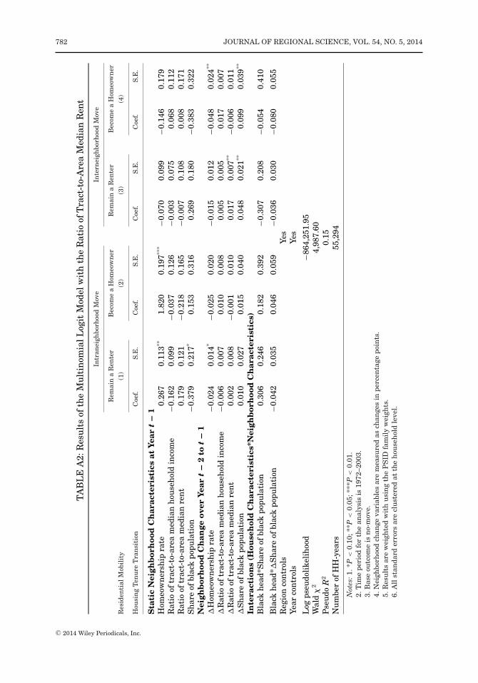
782 JOURNAL OF REGIONAL SCIENCE, VOL. 54, NO. 5, 2014
TA
BL
EA
2:R
esu
lts
ofth
eM
ult
inom
ialL
ogit
Mod
elw
ith
the
Rat
ioof
Tra
ct-t
o-A
rea
Med
ian
Ren
t
Intr
anei
ghbo
rhoo
dM
ove
Inte
rnei
ghbo
rhoo
dM
ove
Rem
ain
aR
ente
rB
ecom
ea
Hom
eow
ner
Rem
ain
aR
ente
rB
ecom
ea
Hom
eow
ner
Res
iden
tial
Mob
ilit
y(1
)(2
)(3
)(4
)
Hou
sin
gT
enu
reT
ran
siti
onC
oef.
S.E
.C
oef.
S.E
.C
oef.
S.E
.C
oef.
S.E
.
Sta
tic
Nei
ghb
orh
ood
Ch
arac
teri
stic
sat
Yea
rt
−1
Hom
eow
ner
ship
rate
0.26
70.
113**
1.82
00.
197**
*−0
.070
0.09
9−0
.146
0.17
9R
atio
oftr
act-
to-a
rea
med
ian
hou
seh
old
inco
me
−0.1
620.
099
−0.0
370.
126
−0.0
030.
075
0.06
80.
112
Rat
ioof
trac
t-to
-are
am
edia
nre
nt
0.17
90.
121
−0.2
180.
165
−0.0
070.
108
0.00
80.
171
Sh
are
ofbl
ack
popu
lati
on−0
.379
0.21
7*0.
153
0.31
60.
269
0.18
0−0
.383
0.32
2N
eigh
bor
hoo
dC
han
geov
erY
ear
t−
2to
t−
1�
Hom
eow
ner
ship
rate
−0.0
240.
014*
−0.0
250.
020
−0.0
150.
012
−0.0
480.
024**
�R
atio
oftr
act-
to-a
rea
med
ian
hou
seh
old
inco
me
−0.0
060.
007
0.01
00.
008
0.00
50.
005
0.01
70.
007
�R
atio
oftr
act-
to-a
rea
med
ian
ren
t0.
002
0.00
8−0
.001
0.01
00.
017
0.00
7**−0
.006
0.01
1�
Sh
are
ofbl
ack
popu
lati
on0.
010
0.02
70.
015
0.04
00.
048
0.02
1**0.
099
0.03
9**
Inte
ract
ion
s(H
ouse
hol
dC
har
acte
rist
ics*
Nei
ghb
orh
ood
Ch
arac
teri
stic
s)B
lack
hea
d*S
har
eof
blac
kpo
pula
tion
0.30
60.
246
0.18
20.
392
−0.3
070.
208
−0.0
540.
410
Bla
ckh
ead*
�S
har
eof
blac
kpo
pula
tion
−0.0
420.
035
0.04
60.
059
−0.0
360.
030
−0.0
800.
055
Reg
ion
con
trol
sYe
sYe
arco
ntr
ols
Yes
Log
pseu
doli
keli
hoo
d−8
64,2
51.9
5W
ald
�2
4,98
7.60
Pse
udo
R2
0.15
Nu
mbe
rof
HH
-yea
rs55
,294
Not
es:1
.*P
<0.
10;*
*P<
0.05
;***
P<
0.01
.2.
Tim
epe
riod
for
the
anal
ysis
is19
72–2
003.
3.B
ase
outc
ome
isn
o-m
ove.
4.N
eigh
borh
ood
chan
geva
riab
les
are
mea
sure
das
chan
ges
inpe
rcen
tage
poin
ts.
5.R
esu
lts
are
wei
ghte
dw
ith
usi
ng
the
PS
IDfa
mil
yw
eigh
ts.
6.A
llst
anda
rder
rors
are
clu
ster
edat
the
hou
seh
old
leve
l.
C© 2014 Wiley Periodicals, Inc.

LEE: WHY DO RENTERS STAY IN OR LEAVE CERTAIN NEIGHBORHOODS? 783
TA
BL
EA
3:C
ompa
riso
ns
ofth
eC
har
acte
rist
ics
ofR
ente
rsR
esid
ing
inH
igh
,Mid
dle,
and
Low
Hom
eow
ner
ship
Nei
ghbo
rhoo
ds
Su
bsam
ple
ofR
ente
rsS
ubs
ampl
eof
Ren
ters
Su
bsam
ple
ofR
ente
rsR
esid
ing
inN
eigh
borh
oods
Res
idin
gin
Nei
ghbo
rhoo
dsR
esid
ing
inN
eigh
borh
oods
wit
hH
igh
Hom
eow
ner
ship
wit
hM
iddl
eH
omeo
wn
ersh
ipw
ith
Low
Hom
eow
ner
ship
Rat
es(1
)R
ates
(2)
Rat
es(3
)
Var
iabl
eM
ean
S.D
.M
ean
S.D
.M
ean
S.D
.
Hou
seh
old
-Lev
elD
emog
rap
hic
Ch
arac
teri
stic
sA
geof
hea
d36
.231
15.3
4937
.361
15.6
9339
.385
15.9
37B
lack
hea
d(1
=ye
s)0.
326
0.46
90.
481
0.50
00.
631
0.48
2F
emal
eh
ead
(1=
yes)
0.35
80.
480
0.42
20.
494
0.52
60.
499
Hea
dm
arri
ed(1
=ye
s)0.
443
0.49
70.
375
0.48
40.
290
0.45
4H
ead
got
mar
ried
this
year
(1=
yes)
0.05
60.
231
0.04
10.
199
0.02
90.
169
Hea
dgo
tdi
vorc
edor
sepa
rate
dth
isye
ar(1
=ye
s)0.
046
0.21
00.
043
0.20
30.
032
0.17
6N
um
ber
ofch
ildr
en0.
920
1.24
11.
024
1.34
41.
038
1.39
0C
hil
dw
asbo
rnth
isye
ar(1
=ye
s)0.
081
0.27
30.
073
0.26
00.
057
0.23
2H
ead’
sed
uca
tion
dum
mie
s(r
efer
ence
=le
ssth
anh
igh
sch
ool)
Hig
hsc
hoo
l0.
497
0.50
00.
546
0.49
80.
546
0.49
8S
ome
coll
ege
edu
cati
on0.
247
0.43
10.
231
0.42
10.
204
0.40
3C
olle
geed
uca
tion
0.18
50.
389
0.13
30.
340
0.12
30.
329
Hou
seh
old
-Lev
elE
con
omic
Ch
arac
teri
stic
sH
ead
un
empl
oyed
(1=
yes)
0.06
40.
244
0.09
50.
293
0.13
70.
343
Per
man
ent
hou
seh
old
inco
me
37.9
2033
.372
31.4
5925
.197
27.8
7423
.633
Tra
nsi
tory
hou
seh
old
inco
me
0.52
323
.510
−0.0
2121
.072
0.18
710
.720
Oth
erH
ouse
hol
d-L
evel
Ch
arac
teri
stic
sH
omeo
wn
ersh
ipex
peri
ence
(ref
eren
ce=
has
alw
ays
been
are
nte
r)W
asev
era
hom
eow
ner
0.72
40.
447
0.59
70.
490
0.40
10.
490
Hom
eow
ner
ship
his
tory
isu
nkn
own
0.16
80.
374
0.23
30.
423
0.36
90.
482
Nu
mbe
rof
year
sre
sidi
ng
inth
ecu
rren
th
ome
2.92
03.
458
3.22
23.
761
3.67
24.
037
Nu
mbe
rof
year
sre
mai
nin
ga
ren
ter
6.74
05.
868
7.51
86.
282
8.33
66.
582
Nu
mbe
rof
room
spe
rpe
rson
2.29
01.
788
2.19
11.
421
2.10
61.
340
Res
idin
gin
sin
gle
fam
ily
un
it(1
=ye
s)0.
469
0.49
90.
398
0.48
90.
235
0.42
4
Con
tin
ued
C© 2014 Wiley Periodicals, Inc.

784 JOURNAL OF REGIONAL SCIENCE, VOL. 54, NO. 5, 2014
TA
BL
EA
3:C
onti
nu
ed
Su
bsam
ple
ofR
ente
rsS
ubs
ampl
eof
Ren
ters
Su
bsam
ple
ofR
ente
rsR
esid
ing
inN
eigh
borh
oods
Res
idin
gin
Nei
ghbo
rhoo
dsR
esid
ing
inN
eigh
borh
oods
wit
hH
igh
Hom
eow
ner
ship
wit
hM
iddl
eH
omeo
wn
ersh
ipw
ith
Low
Hom
eow
ner
ship
Rat
es(1
)R
ates
(2)
Rat
es(3
)
Var
iabl
eM
ean
S.D
.M
ean
S.D
.M
ean
S.D
.
Sta
tic
Nei
ghb
orh
ood
Ch
arac
teri
stic
sat
Yea
rt
−1
Hom
eow
ner
ship
rate
0.82
70.
066
0.62
30.
061
0.29
80.
142
Rat
ioof
trac
t-to
-are
am
edia
nh
ouse
hol
din
com
e1.
097
0.42
60.
879
0.30
70.
640
0.28
4S
har
eof
blac
kpo
pula
tion
0.20
50.
319
0.34
70.
376
0.51
20.
392
Nei
ghb
orh
ood
Ch
ange
over
Yea
rt
−2
tot
−1
�H
omeo
wn
ersh
ipra
te−0
.001
0.02
0−0
.002
0.01
6−0
.001
0.01
5�
Rat
ioof
trac
t-to
-are
am
edia
nh
ouse
hol
din
com
e−0
.002
0.05
3−0
.007
0.04
0−0
.011
0.03
0�
Sh
are
ofbl
ack
popu
lati
on0.
004
0.01
40.
005
0.01
40.
003
0.01
4In
tera
ctio
ns
(Hou
seh
old
Ch
arac
teri
stic
s*N
eigh
bor
hoo
dC
har
acte
rist
ics)
Bla
ckh
ead*
Sh
are
ofbl
ack
popu
lati
on0.
179
0.32
40.
308
0.39
00.
463
0.42
5B
lack
hea
d*�
Sh
are
ofbl
ack
popu
lati
on0.
003
0.01
30.
004
0.01
30.
002
0.01
3
Nu
mbe
rof
HH
-yea
rs9,
178
16,8
6429
,252
Not
e:G
rou
psar
ede
term
ined
byth
eor
der
ofqu
anti
le.T
wo
poin
tsu
sed
are
51.9
and
73.4
perc
ent.
C© 2014 Wiley Periodicals, Inc.

LEE: WHY DO RENTERS STAY IN OR LEAVE CERTAIN NEIGHBORHOODS? 785
REFERENCESAdams, Terry K. 1991. Documentation for 1970 and 1980 Census Extract Datasets. Ann Arbor, MI: Institute for
Social Research, University of Michigan.Bailey, Nick and Mark Livingston. 2007. Population Turnover and Area Deprivation. Bristol: Policy Press.Bayer, Patrick, Marcus D. Casey, Fernando Ferreira, and Robert McMillan. 2012. “Estimating Racial Price
Differentials in the Housing Market,” NBER Working Paper No. 18069.Briggs, Xavier de Souza. 2005. “More Pluribus, Less Unum? The Changing Geography of Race and Opportu-
nity,” In The Geography of Opportunity: Race and Housing Choice in Metropolitan America. Washington, DC,Brookings Institution Press.
Card, David, Alexandre Mas, and Jesse Rothstein. 2008. “Tipping and the Dynamics of Segregation,” QuarterlyJournal of Economics, 123(1), 177–218.
Chamberlain, Gary. 1980. “Analysis of Covariance with Qualitative Data,” Review of Economic Studies, 47,225–238.
Clapp, John M., Anupam Nanda, and Stephen L. Ross. 2008. “Which School Attributes Matter? The Influence ofSchool District Performance and Demographic Composition on Property Values,” Journal of Urban Economics,63(2), 451–466.
Clark, William A.V. 1992. “Residential Preferences and Residential Choices in a Multiethnic Context,” Demogra-phy, 29(3), 451–466.
Clark, William A.V., Marinus Deurloo, and Frans M. Dieleman. 2006. “Residential Mobility and NeighbourhoodOutcomes,” Housing Studies, 21(3), 232–342.
Clark, William A.V. and Frans M. Dieleman. 1996. Households and Housing: Choice and Outcomes in the HousingMarket. New Brunswick, NJ: Center for Urban Policy Research.
Coleman, James S. 1988. “Social Capital in the Creation of Human Capital,” American Journal of Sociology, 94,S95–S120.
———. 1990. Foundations of Social Theory. Cambridge, MA: Harvard University Press.Crowder, Kyle. 2000. “The Racial Context of White Mobility: An Individual-Level Assessment of the White Flight
Hypothesis,” Social Science Research, 29, 223–257.Crowder, Kyle and Scott J. South. 2008. “Spatial Dynamics of White Flight: The Effects of Local and Extralocal
Racial Conditions on Neighborhood Out-Migration,” American Sociological Review, 73, 792–812.David, Quentin, Alexandre Janiak, and Etienne Wasmer. 2008. “Local Social Capital and Geographical Mobility:
A Theory,” IZA Discussion Paper No. 3668.Dawkins, Casey J. 2005. “Racial Gaps in the Transition to First-Time Homeownership: The Role of Residential
Location,” Journal of Urban Economics, 58, 537–554.Deng, Yongheng, Stephen L. Ross, and Susan M. Wachter. 2003. “Racial Differences in Homeownership: The
Effect of Residential Location,” Regional Science and Urban Economics, 33, 517–556.Dieleman, Frans M. 2001. “Modelling Residential Mobility; A Review of Recent Trends in Research,” Journal of
Housing and the Built Environment, 16(3-4), 249–265.Dieleman, Frans M., William A.V. Clark, and Marinus C. Deurloo. 2000. “The Geography of Residential Turnover
in 27 large US Metropolitan Housing Markets, 1985–1995,” Urban Studies, 37(2), 223–245.Ellen, Ingrid Gould. 2000. “Race-Based Neighbourhood Projection: A Proposed Framework for Understanding
New Data on Racial Integration,” Urban Studies, 37(9), 1513–1533.Ellen, Ingrid Gould and Katherine M. O’Regan. 2011. “How Low Income Neighborhoods Change: Entry, Exit, and
Enhancement,” Regional Science and Urban Economics, 41(2), 89–97.Feijten, Peteke and Maarten van Ham. 2009. “Neighbourhood Change . . . Reason to Leave?” Urban Studies,
46(10), 2103–2122.Fitzgerald, John, Peter Gottschalk, and Robert A. Moffitt. 1998. “The Impact of Attrition in the Panel Study Of
Income Dynamics On Intergenerational Analysis,” Journal of Human Resources, 33(2), 300–344.Freeman, Lance. 2005. “Displacement or Succession? Residential Mobility in Gentrifying Neighborhoods,” Urban
Affairs Review, 40(4), 463–491.Freeman, Lance and Frank Braconi. 2004. “Gentrification and Displacement: New York City in the 1990s,”
Journal of the American Planning Association, 70(1), 39–52.Gabriel, Stuart A. and Gary Painter. 2008. “Mobility, Residential Location and the American Dream: The In-
trametropolitan Geography of Minority Homeownership,” Real Estate Economics, 36(3), 499–531.Galster, George C. 1987. Homeowners and Neighbourhood Reinvestment. Durham, NC: Duke University Press.Galster, George C., Roger Andersson, and Sako Musterd. 2010. “Who Is Affected by Neighbourhood Income Mix?
Gender, Age, Family, Employment and Income Differences,” Urban Studies, 47(14), 2915–2944.Galster, George C., Roger Andersson, Sako Musterd, and Timo M. Kauppinen. 2008. “Does Neighborhood Income
Mix Affect Earnings of Adults? New Evidence from Sweden,” Journal of Urban Economics, 63(3), 858–870.Ginther, Donna, Robert Haveman, and Barbara Wolfe. 2000. “Neighborhood Attributes as Determinants of Chil-
dren’s Outcomes: How Robust Are the Relationships?” Journal of Human Resources, 35, 603–642.Greene, William. 2002. “The Behavior of the Fixed Effects Estimator in Nonlinear Models,” From archive.nyu.edu.
C© 2014 Wiley Periodicals, Inc.

786 JOURNAL OF REGIONAL SCIENCE, VOL. 54, NO. 5, 2014
Hagan, John, Ross MacMillan, and Blair Wheaton. 1996. “New Kid in Town: Social Capital and the Life CourseEffects of Family Migration on Children,” American Sociological Review, 61(3), 368–385.
Harris, David R. 1999. “Property Values Drop When Blacks Move in, because . . . : Racial and SocioeconomicDeterminants of Neighbourhood Desirability,” American Sociological Review, 64(3), 461–479.
Hartman, Chester. 1979. “Comment on Neighborhood Revitalization and Displacement: A Review of the Evi-dence,” Journal of the American Planning Association, 45(4), 488–492.
Haurin, Donald R., Robert D. Dietz, and Bruce A. Weinberg. 2005. “The Impact of Neighborhood HomeownershipRates: A Review of the Theoretical and Empirical Literature,” Economics of Innovation and New Technology,14(5), 119–152.
Hilber, Christian A.L. 2005. “Neighbourhood Externality Risk and the Homeownership Status of Properties,”Journal of Urban Economics, 57(2), 213–241.
Ihlanfeldt, Keith R. and Benjamin Scafidi. 2001. “Black Self-segregation as a Cause of Housing Segregation:Evidence from the Multi-City Study of Urban Inequality,” Journal of Urban Economics, 51, 366–390.
Ioannides, Yannis M. and Kamhon Kan. 1996. “Structural Estimation of Residential Mobility and Housing TenureChoice,” Journal of Regional Science, 36(3), 335–363.
Ioannides, Yannis M. and Giorgio Topa. 2010. “Neighborhood Effects: Accomplishments and Looking BeyondThem,” Journal of Regional Science, 50(1), 343–362.
Ioannides, Yannis M. and Jeffrey E. Zabel. 2003. “Neighborhood Effects and Housing Demand,” Journal of AppliedEconometrics, 18(5), 563–584.
Kan, Kamhon. 2000. “Dynamic Modeling of Housing Tenure Choice,” Journal of Urban Economics, 48(1), 46–69.———. 2007. “Residential Mobility and Social Capital,” Journal of Urban Economics, 61(3), 436–457.Katz, Ethan. 2001. “Bias in Conditional and Unconditional Fixed Effects Logit Estimation,” Political Analysis,
9(4), 379–384.Lee, Barrett A., R. Salvador Oropresa, and James W. Kanan. 1994. “Neighborhood Context and Residential
Mobility,” Demography, 31(2), 249–270.Manski, Charles F. 1993. “Identification of Endogenous Social Effects: The Reflection Problem,” The Review of
Economic Studies, 60(3), 531–542.Massey, Douglas S. and Nancy Denton. 1993. American Apartheid: Segregation and the Making of the Underclass.
Cambridge, MA: Harvard University Press.Massey, Douglas S., Andrew B. Gross, and Kumiko Shibuya. 1994. “Migration, segregation, and the geographic
concentration of poverty,” American Sociological Review, 59(3), 425–445.McKinnish, Terra, Randall Walsh, and T. Kirk White. 2010. “Who Gentrifies Low-Income Neighborhoods?” Journal
of Urban Economics, 67(2), 180–193.Parkes, Alison and Ade Kearns. 2003. “Residential Perceptions and Housing Mobility in Scotland: An Analysis of
the Longitudinal Scottish House Condition Survey 1991–96,” Housing Studies, 18, 673–701.Quigley, John M. and Daniel H. Weinberg. 1977. “Intra-Urban Residential Mobility: A Review and Synthesis,”
International Regional Science Review, 2, 41–66.Quillian, Lincoln. 1999. “Migration Patterns and the Growth of High-Poverty Neighbourhoods, 1970–1999,”
American Journal of Sociology, 105, 1–37.———. 2002. “Why Is Black-White Residential Segregation So Persistent? Evidence on Three Theories from
Migration Data,” Social Science Research, 31, 197–229.———. 2003. “How Long Are Exposures to Poor Neighbourhoods? The Long-Term Dynamics of Entry and Exit
from Poor Neighbourhoods,” Population Research and Policy Review, 22, 221–249.Rohe, William M. and Leslie S. Stewart. 1996. “Home Ownership and Neighborhood Stability,” Housing Policy
Debate, 7(1), 37–81.Rosenthal, Stuart S. 2008. “Old Homes, Externalities, and Poor Neighborhoods. A Model of Urban Decline and
Renewal,” Journal of Urban Economics, 63(3), 816–840.Sampson, Robert J., Stephen W. Raudenbush, and Felton Earls. 1997. “Neighbourhoods and Violent Crime: A
Multilevel Study of Collective Efficacy,” Science, 277, 918–924.Schelling, Thomas C. 1969. “Models of Segregation,” The American Economic Review, 59, 488–493.Seko, Miki and Kazuto Sumita. 2007. “Effects of Government Policies on Residential Mobility in Japan: Income
Tax Deduction System and the Rental Act,” Journal of Housing Economics, 16(2), 167–188.Shaw, Clifford Robe and Henry Donald McKay. 1969. Juvenile Delinquency and Urban Areas: A Study of Rates
of Delinquency in Relation to Differential Characteristics of Local Communities in American Cities, revisededition. Chicago, IL: University of Chicago Press.
Simmons, Roberta G., Richard Burgeson, Steven Carlton-Ford, and Dale A. Blyth. 1987. “The Impact of Cumula-tive Change in Early Adolescence,” Child Development, 58(5), 1120–1134.
Smith, Neil. 1996. New Urban Frontier: Gentrification and the Revanchist City. London: Routledge.South, Scott J. and Kyle D. Crowder. 1997. “Residential Mobility Between Cities and Suburbs: Race, Suburban-
ization and Back-to-the-City Moves,” Demography, 34(4), 525–538.
C© 2014 Wiley Periodicals, Inc.

LEE: WHY DO RENTERS STAY IN OR LEAVE CERTAIN NEIGHBORHOODS? 787
Speare, Alden, Sidney Goldstein, and William H. Frey. 1975. Residential Mobility, Migration and MetropolitanChange. Cambridge, MA: Ballinger Publishing Company.
Taub, Richard P., D. Garth Taylor, and Jan D. Dunham. 1984. Paths of Neighborhood Change. Chicago, IL:University of Chicago Press.
Turner, Margery A., Stephen Ross, George C. Galster, and John Yinger. 2002. Discrimination in metropolitanhousing markets: national results from phase 1 of the housing discrimination study (HDS). Washington, DC:U.S. Department of Housing and Urban Development.
van Ham, Maarten and William A.V. Clark. 2009. “Neighbourhood Mobility in Context: Household Moves andChanging Neighbourhoods in the Netherlands,” Environment and Planning A, 41, 1442–1459.
Vigdor, Jacob L., Douglas S. Massey, and Alice M. Rivlin. 2002. “Does Gentrification Harm the Poor? [withComments],” Brookings-Wharton Papers on Urban Affairs, 133–182.
Weinberg, Bruce A., Patricia B. Reagan, and Jeffrey J. Yankow. 2004. “Do Neighborhoods Affect Hours Worked?Evidence from Longitudinal Data,” Journal of Labor Economics, 22(4), 891–924.
Yinger, John. 1995. Closed Doors, Opportunities Lost: The Continuing Costs of Housing Discrimination. New York,NY: Russell Sage Foundation.
Yinger, John. 1998. “Evidence on Discrimination in Consumer Markets,” Journal of Economic Perspectives, 12(Spring), 23–40.
C© 2014 Wiley Periodicals, Inc.


