Download - William M. W I

Statistical Object Recognition
William M. Wells III
Copyright c Massachusetts Insti tute of Technology, 1993

Statistical Object Recognition
by
William Mercer Wells III
Submitted to the Department of Electrical Engineering andComputer Science
onNovember 24, 1992, in partial ful�l lment of therequirements for the degree of
Doctor of Phi losophy
Abstract
To be practical , recognition systems must deal with uncertainty. Positions of imagefeatures inscenes vary. Features sometimes fai l to appear because of unfavorable i l lu-
mination. In this work, methods of statistical inference are combinedwith empiricalmodels of uncertaintyinorder to evaluate andre�ne hypotheses about the occurrenceof a knownobject in a scene.
Probabi l i stic models are used to characterize image features and their correspon-dences. A statistical approach is taken for the acquisi tion of object models from
observations in images: Mean Edge Images are used to capture object features thatare reasonably stable with respect to variations in i l lumination.
The Al ignment approachto recognition, that has beendescribedbyHuttenlocher
andUl lman, is used. The mechanisms that are employedto generate initial hypothe-ses are distinct fromthose that are used to veri fy (and re�ne) them. In this work,posterior probabi l i ty and MaximumLikel ihood are the cri teria for evaluating and
re�ning hypotheses. The recognition strategy advocated in this work may be sum-marizedas Align Re�ne Veri fy, whereby local searchinpose space is uti l izedto re�ne
hypotheses fromthe al ignment stage before veri�cation is carried out.Two formulations of model -based object recognition are described. MAPModel
Matching evaluates joint hypotheses of match and pose, whi le Posterior Marginal
Pose Estimation evaluates the pose only. Local search in pose space is carried out
with the Expectation{Maximization (EM) algorithm.Recognition experiments are describedwhere the EMalgorithmis used to re�ne
andevaluate pose hypotheses in2Dand3D. Initial hypotheses for the 2Dexperimentswere generated by a simple indexing method: Angle Pair Indexing. The Linear
Combination of Views method of Ul lman and Basri i s employed as the projection
model in the 3Dexperiments.
Thesis Supervisor: W. Eric L. Grimson
Title: Associate Professor of Electrical Engineering andComputer Science
2

3
Acknowledgments
I feel fortunate tohavehadProfessor W. Eric L. Grimsonas mythesis advisor, mentor
and friend. His deep knowledge was a tremendous asset. His sharp instincts and
thoughtful guidance helpedme to stay focussedonthe problemof object recognition,
whi le his support and generous advising style provided me the freedomto �nd and
solve my ownproblems.
I appreciate the helpo�eredbymyreading committee, Professors Tomas Lozano-
P�erez, Je�rey Shapiro and Shimon Ullman. Their insights and critici smimproved
mywork. Inparticular, I thankProfessor Shapiro for o�ering his time and statistical
experti se. His contribution to my researchwent wel l beyondhis close reading of my
thesis. Among his valuable suggestions was use of the EMalgorithm. In thanking
the above committee, however, I claimany errors or inconsistencies as my own.
I feel lucky for my years at MIT. I have enjoyed Professor Grimson's research
group. I learnedmuchabout recognitionfrom: TaoAlter, ToddCass, DavidClemens,
David Jacobs, Karen Sarachick, Tanveer Syeda and Steve White as wel l as Amnon
Shashua. Inmoving on, I shal l miss working with such a critical mass of talent, and
beyond this, I knowI shal l miss themas friends.
My early days at the AI Lab were spent in Professor Rodney Brook's robotics
group. There, I learneda lot working onSquirt the robot fromhimandAnita Flynn.
I appreciate their continuedfriendship. I foundmuchto admire inthemas col leagues.
I also thank Flynn for her assi stance with some experimental work in this thesis.
In the AI Labas a whole, I enjoyedmycontacts withPaul Viola, Professors Tom
Knight andBertholdHorn, andothers toonumerous tomention. Sundar Narasimhan,
Jose Robles andPat O'Donnel l provided invaluable assi stance with the Puma robot.
Grimson's administrative assi stant, Jeanne Speckman, was terri�c. I thankProfessor
PatrickWinston, director of the AI Lab, for providing the unique environment that
the AI Lab is. My stay has been a happy one.
I spent three summers as a student at MITLincoln Laboratory in Group 53.

4
Groupleader Al Gschwendtner providedsupport andagoodenvironment for pursuing
some of the research found in this thesis. There, I enjoyedcol laborating withMural i
Menon on image restoration, and learned some things about the EMalgorithmfrom
TomGreen. Steve Rak helped prepare the range images used inChapter 7.
Prior to MIT, I worked with Stan Rosenschein at SRI International and Teleos
Research. The earl iest incarnation of this research originated during those years.
Rosenschein led a mobi le robot group comprised of Lesl ie Kaelbl ing, Stanley Rei fel ,
mysel f andmore looselyof Stuart Shieber andFernandoPereira. Workingwiththem,
I learned howenjoyable researchcan be.
Professor Thomas O. Binford at StanfordUniversi ty introducedme to computer
vision. There, I foundstimulatingcontacts inDavidLowe, DavidMarimont, Professor
BrianWandel l andChristopher Goad. After Stanford, my �rst opportunity to work
on computerized object recognition was withGoad at Si lma Incorporated.
I owe much to myparents who have always been there to support and encourage
me. My time at the AI Labwouldnot have been possible without them.
And �nal ly, this work depended dai ly upon the love and support of my wife,
Col leenGi l lard, and daughters, Georgia andWhitney, who wi l l soon be seeing more
of me.
This researchwas supported in part by the AdvancedResearchProjects Agency
of the Department of Defense under Armycontract number DACA76-85-C-0010 and
under O�ce of Naval Researchcontracts N00014-85-K-0124 andN00014-91-0J-4038.

5
To Col leen, Georgia andWhitney

6

Content s
1 Introduction 11
1.1 The Problem : : : : : : : : : : : : : : : : : : : : : : : : : : : : : : : 11
1.2 The Approach : : : : : : : : : : : : : : : : : : : : : : : : : : : : : : : 13
1.2.1 Statistical Approach : : : : : : : : : : : : : : : : : : : : : : : 13
1.2.2 Feature-BasedRecognition : : : : : : : : : : : : : : : : : : : : 14
1.2.3 Al ignment : : : : : : : : : : : : : : : : : : : : : : : : : : : : : 15
1.3 Guide to Thesis : : : : : : : : : : : : : : : : : : : : : : : : : : : : : : 18
2 Modeling Feature Correspondence 21
2.1 Features andCorrespondences : : : : : : : : : : : : : : : : : : : : : : 21
2.2 An Independent Correspondence Model : : : : : : : : : : : : : : : : : 24
2.3 AMarkovCorrespondence Model : : : : : : : : : : : : : : : : : : : : 25
2.4 Incorporating Sal iency : : : : : : : : : : : : : : : : : : : : : : : : : : 27
2.5 Conclusions : : : : : : : : : : : : : : : : : : : : : : : : : : : : : : : : 28
3 Model ing Image Features 29
3.1 AUniformModel for BackgroundFeatures : : : : : : : : : : : : : : : 30
3.2 ANormal Model for MatchedFeatures : : : : : : : : : : : : : : : : : 30
3.2.1 Empirical Evidence for the Normal Model : : : : : : : : : : : 31
3.3 OrientedStationary Statistics : : : : : : : : : : : : : : : : : : : : : : 40
3.3.1 Estimating the Parameters : : : : : : : : : : : : : : : : : : : : 40
7
8 CONTENTS
3.3.2 Special izing the Covariance : : : : : : : : : : : : : : : : : : : 42
4 Model ing Objects 43
4.1 Monol i thic 3DObject Models : : : : : : : : : : : : : : : : : : : : : : 43
4.2 Interpolation of Views : : : : : : : : : : : : : : : : : : : : : : : : : : 45
4.3 Object Models fromObservation : : : : : : : : : : : : : : : : : : : : 46
4.4 MeanEdge Images : : : : : : : : : : : : : : : : : : : : : : : : : : : : 47
4.5 Automatic 3DObject Model Acquisi tion : : : : : : : : : : : : : : : : 50
5 Model ing Projection 57
5.1 Linear ProjectionModels : : : : : : : : : : : : : : : : : : : : : : : : : 57
5.2 2DPoint Feature Model : : : : : : : : : : : : : : : : : : : : : : : : : 58
5.3 2DPoint-Radius Feature Model : : : : : : : : : : : : : : : : : : : : : 59
5.4 2DOriented-Range Feature Model : : : : : : : : : : : : : : : : : : : 61
5.5 Linear Combinationof Views : : : : : : : : : : : : : : : : : : : : : : 61
6 MAPModel Matching 65
6.1 Objective Function for Pose andCorrespondences : : : : : : : : : : : 66
6.1.1 Using the MarkovCorrespondence Model : : : : : : : : : : : : 72
6.2 Experimental Implementation : : : : : : : : : : : : : : : : : : : : : : 72
6.2.1 Search inCorrespondence Space : : : : : : : : : : : : : : : : : 73
6.2.2 Example SearchResults : : : : : : : : : : : : : : : : : : : : : 75
6.3 Search inPose Space : : : : : : : : : : : : : : : : : : : : : : : : : : : 79
6.4 Extensions : : : : : : : : : : : : : : : : : : : : : : : : : : : : : : : : : 84
6.5 RelatedWork : : : : : : : : : : : : : : : : : : : : : : : : : : : : : : : 84
6.6 Summary : : : : : : : : : : : : : : : : : : : : : : : : : : : : : : : : : 86
7 Posterior Marginal Pose Estimation 87
7.1 Objective Function for Pose : : : : : : : : : : : : : : : : : : : : : : : 88
7.2 Using the MarkovCorrespondence Model : : : : : : : : : : : : : : : : 91

CONTENTS 9
7.3 Range Image Experiment : : : : : : : : : : : : : : : : : : : : : : : : : 95
7.3.1 Preparation of Features : : : : : : : : : : : : : : : : : : : : : : 95
7.3.2 Sampl ing The Objective Function : : : : : : : : : : : : : : : : 99
7.4 Video Image Experiment : : : : : : : : : : : : : : : : : : : : : : : : : 105
7.4.1 Preparation of Features : : : : : : : : : : : : : : : : : : : : : : 105
7.4.2 Search inPose Space : : : : : : : : : : : : : : : : : : : : : : : 105
7.4.3 Sampl ing The Objective Function : : : : : : : : : : : : : : : : 105
7.5 Relation to Robust Estimation : : : : : : : : : : : : : : : : : : : : : : 108
7.5.1 Connection to Neural Network Sigmoid Function : : : : : : : 112
7.6 PMPEE�ciency Bound : : : : : : : : : : : : : : : : : : : : : : : : : 115
7.7 RelatedWork : : : : : : : : : : : : : : : : : : : : : : : : : : : : : : : 119
7.8 Summary : : : : : : : : : : : : : : : : : : : : : : : : : : : : : : : : : 122
8 Expectation { MaximizationAlgorithm 123
8.1 De�nition of EMIteration : : : : : : : : : : : : : : : : : : : : : : : : 123
8.2 Convergence : : : : : : : : : : : : : : : : : : : : : : : : : : : : : : : : 127
8.3 Implementation Issues : : : : : : : : : : : : : : : : : : : : : : : : : : 127
8.4 RelatedWork : : : : : : : : : : : : : : : : : : : : : : : : : : : : : : : 128
9 Angle Pair Indexing 129
9.1 Description of Method : : : : : : : : : : : : : : : : : : : : : : : : : : 129
9.2 Sparsi�cation : : : : : : : : : : : : : : : : : : : : : : : : : : : : : : : 132
9.3 RelatedWork : : : : : : : : : : : : : : : : : : : : : : : : : : : : : : : 132
10 Recognition Experiments 135
10.1 2DRecognitionExperiments : : : : : : : : : : : : : : : : : : : : : : : 135
10.1.1 Generating Al ignments : : : : : : : : : : : : : : : : : : : : : : 139
10.1.2 Scoring Indexer Al ignments : : : : : : : : : : : : : : : : : : : 140
10.1.3 Re�ning Indexer Al ignments : : : : : : : : : : : : : : : : : : : 140
10.1.4 Final EMWeights : : : : : : : : : : : : : : : : : : : : : : : : 144

10 CONTENTS
10.2 Evaluating RandomAlignments : : : : : : : : : : : : : : : : : : : : : 145
10.3 Convergence withOcclusion : : : : : : : : : : : : : : : : : : : : : : : 148
10.4 3DRecognitionExperiments : : : : : : : : : : : : : : : : : : : : : : : 148
10.4.1 Re�ning 3DAlignments : : : : : : : : : : : : : : : : : : : : : 148
10.4.2 Re�ning PerturbedPoses : : : : : : : : : : : : : : : : : : : : : 157
11 Conclusions 163
ANotation 165
References 168

Chapt er 1
Int r oduct ion
Visual object recognition is the focus of the researchreported inthis thesis. Recogni -
tionmust deal withuncertaintyto be practical . Positions of image features belonging
to objects in scenes vary. Features sometimes fai l to appear because of unfavorable
i l lumination. In this work, methods of statistical inference are combinedwith empir-
ical models of uncertainty in order to evaluate hypotheses about the occurrence of a
knownobject ina scene. Other problems, suchas the generationof initial hypotheses
and the acquisi tion of object model features are also addressed.
1.1 The Problem
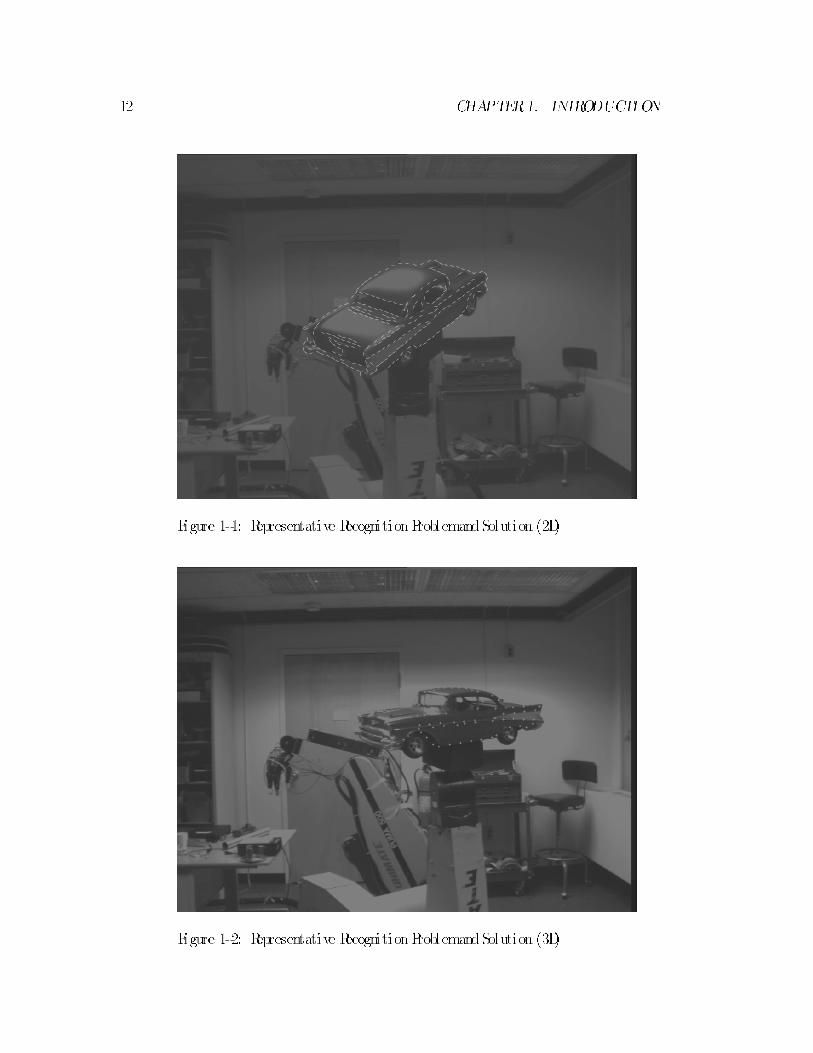
Representative recognitionproblems and their solutions are i l lustrated inFigures 1-1
and1-2. The problemis to detect and locate the car indigitized video images, using
previouslyavai lable detai ledinformationabout the car. Inthese �gures, object model
features are superimposedover the video images at the positionandorientationwhere
the car was found. Figure 1-1 shows the results of 2Drecognition, whi le Figure 1-2
i l lustrates the results of 3Drecognition. These images are fromexperiments that are
described in Chapter 10. Practical solutions to problems l ike these wi l l improve the
exibi l i ty of robotic systems.
11
12 CHAPTER1. INTRODUCTION
Figure 1-1: Representative RecognitionProblemandSolution (2D)
Figure 1-2: Representative RecognitionProblemandSolution (3D)

1. 2. THEAPPROACH 13
Inthis work, the recognitionproblemis restrictedto�ndingoccurrences of a single
object in scenes that may containother unknownobjects. Despite the simpl i�cation
and years of research, the problemremains largely unsolved. Robust systems that
canrecognize smoothobjects having sixdegrees of freedomof position, under varying
conditions of i l lumination, occlusion, andbackground, are not commercial lyavai lable.
Much e�ort has been expended on this problemas is evident in the comprehensive
reviews of research in computer-based object recognition by Besl and Jain [5], who
cited 203 references, and Chin and Dyer [18] , who cited 155 references. The goal of
this thesis i s to characterize, as wel l as to describe howto �nd, robust solutions to
visual object recognition problems.
1.2 The Approach
In this work, statistical methods are used to evaluate and re�ne hypotheses inobject
recognition. Angle Pair Indexing, a means of generating hypotheses, i s introduced.
These mechanisms are used inanextensionof the Al ignment method that includes a
pose re�nement step. Eachof these components are ampl i�ed below.
1.2.1 Statistical Approach
Inthis research, visual object recognitionis approachedviathe principles of Maximum
Likel ihood (ML) and MaximumA-Posteriori probabi l i ty (MAP). These principles,
along with speci�c probabi l i stic models of aspects of object recognition, are used to
derive objective functions for evaluatingandre�ning recognitionhypotheses. TheML
andMAPcriteriahave alonghistoryof successful appl icationinformulatingdecisions
and in making estimates fromobserved data. They have attractive properties of
optimal i ty and are often useful whenmeasurement errors are signi�cant.
In other areas of computer vision, statistics has proven useful as a theoretical
framework. The work of Yui l le, Geiger and B�ultho� on stereo [78] i s one example,
14 CHAPTER1. I NTRODUCTION
whi le in image restoration the work of Geman andGeman [28] , Marroquin [54] , and
Marroquin, Mitter and Poggio [55] are others. The statistical approach that is used
in this thesis converts the recognition probleminto a wel l de�ned (althoughnot nec-
essari ly easy) optimization problem. This has the advantage of providing an expl ici t
characterizationof the problem, whi le separating it fromthe description of the algo-
ri thms used to solve it. Adhoc objective functions have beenpro�tablyused insome
areas of computer vision. Such an approach is used by Barnard in stereo matching
[2] , Blake andZisserman [7] in image restoration andBeveridge, Weiss andRiseman
[6] in l ine segment based model matching. With this approach, plausible forms for
components of the objective function are often combinedusing trade-o�parameters.
Such trade-o�parameters are determined empirical ly. An advantage of deriving ob-
jective functions fromstatistical theories i s that assumptions become expl ici t { the
forms of the objective functioncomponents are clearly relatedto speci�c probabi l i stic
models. If these models �t the domainthenthere is some assurance that the resulting
cri teria wi l l performwel l . Asecondadvantage is that the trade-o�parameters in the
objective function can be derived frommeasurable statistics of the domain.
1.2.2 Feature-Based Recognition
This workuses a feature-based approachto object recognition. Features are abstrac-
tions l ike points or curves that summarize some structure of the patterns inanimage.
There are several reasons for using feature based approaches to object recognition.
� Features can concisely represent objects and images. Features derived from
brightness edges cansummarize the important events of an image inawaythat
is reasonably stable with respect to scene i l lumination.
� In the al ignment approach to recognition (to be described shortly), hypotheses
are veri�edby projecting the object model into the image, then comparing the
prediction against the image. By using compact, feature-based representations

1. 2. THEAPPROACH 15
of the object, projection costs may be kept low.
� Features also faci l i tate hypothesis generation. Indexing methods are attractive
mechanisms for hypothesis generation. Such methods use tables indexed by
properties of smal l groups of image features to quickly locate corresponding
model features.
Object Features fromObservation
Amajor issue that must be faced in model -based object recognition concerns the
origin of the object model i tsel f. The object features that are used in this work are
derivedfromactual image observations. This methodof feature acquisi tionautomat-
ical ly favors those features that are l ikely to be detected in images. The potential ly
di�cult problemof predicting image features fromabstract geometric models i s by-
passed. This prediction problemis manageable in some constrained domains (with
polyhedral objects, for instance) but it i s often di�cult, especial ly with smooth ob-
jects, lowresolution images and l ighting variations.
For robustness, simple local image features are used in this work. Features of this
sort are easi ly detected in contrast to extended features l ike l ine segments. Extended
features have been used in some systems for hypothesis generation because their ad-
ditional structure provides more constraint thanthat o�eredbysimple local features.
Extended features, nonetheless, have drawbacks in being di�cult to detect due to
occlusions and local ized fai lures of image contrast. Because of this, systems that rely
on distinguished features can lose robustness.
1.2.3 Alignment
Hypothesize-and-test, or alignment methods have proven e�ective in visual object
recognition. Huttenlocher and Ul lman [43] used search over minimal sets of corre-
sponding features to establ i sh candidate hypotheses. In their work these hypotheses,

16 CHAPTER1. I NTRODUCTION
or al i gnments, are tested by projecting the object model into the image using the
pose (position and orientation) impl ied by the hypothesis, and then by performing a
detai led comparison with the image. The basic strategy of the al ignment method is
to use separate mechanisms for generating and testing hypotheses.
Recently, indexing methods have become avai lable for e�ciently generating hy-
potheses in recognition. These methods avoida signi�cant amount of searchbyusing
pre-computed tables for looking up the object features that might correspond to a
groupof image features. The geometric hashingmethodof LamdanandWolfson[49]
uses invariant properties of smal l groups of features under a�ne transformations as
the look-up key. Clemens and Jacobs [19] [20] , and Jacobs [45] described indexing
methods that gain e�ciency by using a feature grouping process to select smal l sets
of image features that are l ikely to belong to one object in the scene.
Inthis work, asimple formof 2Dindexing, Angl e Pai r I ndexi ng, i s usedtogenerate
initial hypotheses. It uses an invariant property of pairs of image features under
translation, rotation and scale. This i s described inChapter 9.
The Hough transform[40] [44] i s another commonly used method for generating
hypotheses in object recognition. In the Houghmethod, feature-based clustering is
performed in pose space, the space of the transformations describing the possible
motion of the object. This method was used by Grimson and Lozano-P�erez [36] to
local ize the search in recognition.
These fast methods of hypothesis generationprovide ongoing reasons for using the
al ignment approach. They are often most e�ective when used in conjunction with
veri�cation. Veri�cation is important because indexing methods can be susceptible
to table col l i sions, whi le Hough methods sometimes generate false positives due to
their aggregationof inconsistent evidence inpose space bins. This last point has been
argued byGrimson andHuttenlocher [35] .
The usual al ignment strategymaybe summarizedas al i gn veri fy. Al ignment and
veri�cation place di�ering pressures on the choice of features for recognition. Mech-

1. 2. THEAPPROACH 17
anisms used for generating hypotheses typical ly have computational complexity that
is polynomial in the number of features involved. Because of this, there is signi�cant
advantage to using lowresolution features { there are fewer of them. Unfortunately,
pose estimates basedon coarse features tend to be less accurate than those based on
high resolution features.
Likewise, veri�cation is usual ly more rel iable with high resolution features. This
approachyields more detai led comparisons. These di�ering pressures maybe accom-
modated by employing coarse-�ne approaches. The coarse-�ne strategy was uti l ized
successful ly in stereo by Grimson [33] . In the coarse-�ne strategy, hypotheses de-
rived fromlow-resolution features l imit the search for hypotheses derived fromhigh-
resolution features. There are some potential di�culties that arise when applying
coarse-�ne methods in conjunction with 3Dobject models. These may be avoided
by using view-based alternatives to 3Dobject model ing. These issues are discussed
more ful ly inChapter 4.
AlignRe�ne Veri fy
The recognition strategy advocated in this work may be summarized as al i gn re�ne
veri f y. This approach has been used by Lipson [50] in re�ning al ignments. The key
observation is that local search in pose space may be used to re�ne the hypothesis
fromthe al ignment stage before veri�cation is carried out. In hypothesize and test
methods, the pose estimates of the initial hypotheses tendtobe somewhat inaccurate,
since theyare basedonminimal sets of corresponding features. Better pose estimates
(hence, better veri�cations) are l ikelyto result fromusingal l supporting image feature
data, rather thana smal l subset. Chapter 8 describes a method that re�nes the pose
estimate whi le simultaneously identi fying and incorporating the constraints of al l
supporting image features.

18 CHAPTER1. I NTRODUCTION
1.3 Guide to Thesis
Brie y, the presentation of the material in this thesis i s essential ly bottom-up. The
early chapters are concernedwith bui lding the components of the formulation, whi le
the main contributions, the statistical formulations of object recognition, are de-
scribed in Chapters 6 and 7. After that, related algorithms are described, fol lowed
by experiments and conclusions.
In more detai l , Chapter 2 describes the probabi l i stic models of the correspon-
dences, or mapping between image features and features belonging to either the ob-
ject or to the background. These models use the principle of maximum-entropywhere
l i ttle information is avai lable before the image is observed. In Chapter 3, probabi l i s-
tic models are developed that characterize the feature detection process. Empirical
evidence is described to support the choice of model .
Chapter 4 discusses a way of obtaining average object edge features froma se-
quence of observations of the object inimages. Deterministic models of the projection
of features into the image are discussed in Chapter 5. The projectionmethods used
in this workare l inear in the parameters of the transformations. Methods for 2Dand
3Dare discussed, including the Linear Combinationof Views method of Ul lmanand
Basri [71] .
InChapter 6 the abovemodels are combinedinaBayesianframeworkto construct
a cri terion, MAP Model Matchi ng, for evaluating hypotheses in object recognition.
In this formulation, complete hypotheses consist of a description of the correspon-
dences between image and object features, as wel l as the pose of the object. These
hypotheses are evaluatedby their posterior (after the image is observed) probabi l i ty.
Arecognitionexperiment is describedthat uses the cri teria to guide a heuristic search
over correspondences. AconnectionbetweenMAPModel Matching andamethodof
robust chamfer matching [47] i s described.
Bui lding on the above, a second criterion is described in Chapter 7: Pos t er i or
Mar gi nal Pos e Es t i mat i on (PMPE). Here, the solution being sought is simply the

1. 3. GUI DETOTHESI S 19
pose of the object. The posterior probabi l i ty of poses is obtained by taking the
formal marginal , over al l possible matches, of the posterior probabi l i ty of the joint
hypotheses of MAPModel Matching. This results in a smooth, non-l inear objective
function for evaluating poses. The smoothness of the objective function faci l i tates
local search in pose space as a mechanismfor re�ning hypotheses in recognition.
Some experimental explorations of the objective function inpose space are described.
These characterizations are carriedout in two domains: video imagery and synthetic
radar range imagery.
Chapter 8 describes use of the the Expectat i on-Maximi zat i on (EM) algorithm[21]
for �nding local maxima of the PMPEobjective function. This algorithmalternates
between the Mstep { a weighted least squares pose estimate, and the Estep { re-
calculation of the weights based on a saturating non-l inear function of the residuals.
This algorithmis used to re�ne and evaluate poses in 2Dand 3Drecognition ex-
periments that are describedinChapter 10. Initial hypotheses for the 2Dexperiments
were generated by a simple indexing method, Angl e Pai r Indexi ng, that is described
inChapter 9 . The Linear Combinationof Views methodof Ul lmanandBasri [71] i s
employed as the projectionmodel in the 3Dexperiments reported there.
Final ly, some conclusions are drawninChapter 11. The notationusedthroughout
is summarized inAppendix A.

20 CHAPTER1. I NTRODUCTION

Chapt er 2
Modeli ng Feat ur e Cor r es pondence
This chapter is concernedwithprobabi l i stic models of feature correspondences. These
models wi l l serve as priors in the statistical theories of object recognition that are
described inChapters 6 and 7, andare important components of those formulations.
Theyare usedtoassess the probabi l i tythat features correspondbefore the image data
is compared to the object model . They capture the expectation that some features
in an image are anticipated to be due to the object
Three di�erent models of feature correspondence are described, one of which is
used in the recognition experiments described inChapters 6, 7, and 10.
2.1 Features andCorrespondences
This research focuses on feature-based object recognition. The object being sought
and the image being analyzed consist of discrete features.
Let the image that is to be analyzed be represented by a set of v-dimensional
point features
Y = fY1; Y2; : : : ; Yng ; Yi 2 Rv:
Image features are discussed inmore detai l inChapters 3 and 5.
21

22 CHAPTER2. MODELI NGFEATURECORRESPONDENCE
The object to be recognized is also described by a set of features,
M =fM 1;M2; : : : ;Mmg :
The features wi l l usual lybe representedbyreal matrices. Additional detai l s onobject
features appears inChapters 4 and 5.
In this work, the interpretation of the features in an image is represented by the
variable �, whichdescribes the mapping fromimage features to object features or the
scene background. This i s also referred to as the cor r es pondences .
�=f� 1;�2; : : : ;�ng ; �i 2M[ f?g :
Inan interpretation, eachimage feature, Y i, wi l l be assignedeither to some object
feature M j, or to the background, which is denoted by the symbol ?. This symbol
plays a role simi lar to that of the nul l character inthe interpretationtrees of Grimson
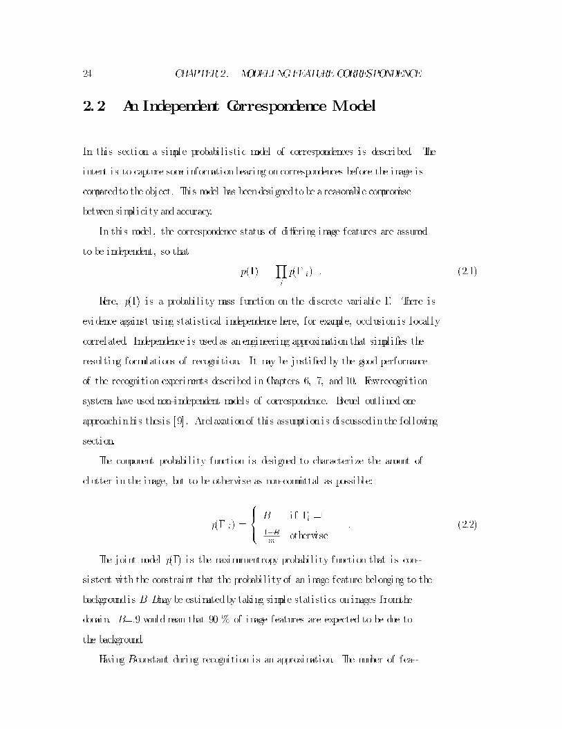
andLozano-P�erez [36] . Aninterpretationis i l lustrated inFigure 2-1. �is a col lection
of variables that is indexed in paral lel with the image features. Each variable � i
represents the assignment of the corresponding image feature Y i. It may take on as
value anyof the object features M j, or the background, ?. Thus, the meaning of the
expression� 5 =M 6 i s that image feature �ve is assignedto object feature six, l ikewise
�7 =?means that image feature seven has been assigned to the background. In an
interpretationeach image feature is assigned, whi le some object features maynot be.
Additional ly, several image features maybe assignedto the same object feature. This
representational lows image interpretations that are implausible { other mechanisms
are used to encourage metrical consistency.

2. 1. FEATURES ANDCORRESPONDENCES 23
Γ⊥
Μ
Μ
Μ
Μ
Μ
Μ
Μ
Μ
Μ
Μ
Μ
Μ
Μ1
2
3
4
5
6
7
8
9
10
11
12
13
Υ1
Υ
Υ
Υ
Υ
Υ
Υ
Υ
Υ
Υ
Υ
2
3
4
5
6
7
8
9
10
11
Figure 2-1: Image Features, Object Features, andCorrespondences
24 CHAPTER2. MODELI NGFEATURECORRESPONDENCE
2.2 An Independent Correspondence Model
In this section a simple probabi l i stic model of correspondences is described. The
intent is to capture some informationbearing oncorrespondences before the image is
comparedto the object. This model has beendesignedtobe a reasonable compromise
between simpl ici ty and accuracy.
In this model , the correspondence status of di�ering image features are assumed
to be independent, so that
p(�) =Yi
p(� i) : (2:1)
Here, p(�) is a probabi l i ty mass function on the discrete variable �. There is
evidence against using statistical independence here, for example, occlusion is local ly
correlated. Independence is used as anengineering approximation that simpl i�es the
resulting formulations of recognition. It may be justi�ed by the good performance
of the recognition experiments described in Chapters 6, 7, and 10. Fewrecognition
systems have used non-independent models of correspondence. Breuel outl ined one
approachinhis thesis [9] . Arelaxationof this assumptionis discussedinthe fol lowing
section.
The component probabi l i ty function is designed to characterize the amount of
clutter in the image, but to be otherwise as non-committal as possible:
p(� i) =
8><>:B i f �i =?1�Bm
otherwise: (2:2)
The joint model p(�) is the maximumentropy probabi l i ty function that is con-
si stent with the constraint that the probabi l i ty of an image feature belonging to the
backgroundis B. Bmaybe estimatedby taking simple statistics on images fromthe
domain. B=:9 wouldmean that 90 % of image features are expected to be due to
the background.
Having Bconstant during recognition is an approximation. The number of fea-
2. 3. AMARKOVCORRESPONDENCEMODEL 25
tures due to the object wi l l l ikelyvaryaccording to the size of the object inthe scene.
Bcouldbe estimatedat recognitiontime bypre-processingmechanisms that evaluate
image clutter, and factor in expectations about the size of the object. In practice,
the approximationworks wel l in control led situations.
The independent correspondence model i s used in the experiments reported in
this research.
2.3 AMarkov Correspondence Model
As indicatedabove, one inaccuracy of the independent correspondence model i s that
sample real izations of � drawn fromthe probabi l i ty function of Equations 2.1 and
2.2 wi l l tend to be overly fragmented in their model ing of occlusion. This section
describes a compromise model that relaxes the independence assumption somewhat
by al lowing the correspondence status of an image feature (� i) to depend on that of
i ts neighbors. In the domain of this research, image features are fragments of image
edge curves. These features have a natural neighbor relation, adjacency along the
image edge curve, that may be used for constructing a 1DMarkov RandomField
(MRF) model of correspondences. MRF's are col lections of randomvariables whose
conditional dependence is restricted to l imited size neighborhoods. MRFmodels are
discussed by Geman and Geman [28] . The fol lowing describes an MRFmodel of
correspondences intended to provide a more accurate model of occlusion.
p(�) =q(� 1)q(� 2) : : : q(� n) r1(�1;�2)r2(�2;�3) : : : rn�1(�n�1;�n) ; (2:3)
where
q(� i) =
8><>:e1 i f �i =?
e2 otherwise(2:4)

26 CHAPTER2. MODELI NGFEATURECORRESPONDENCE
and
ri(a; b) =
8>>>>>>>><>>>>>>>>:
8>>>>><>>>>>:e3 i f a=?andb=?
e4 i f a 6=?andb 6 =?
e5 otherwise
9>>>>>=>>>>>;i f features i and i+ 1 are neighbors
1 otherwise :
(2:5)
The assignment of indices to image features should be done in such a way that
neighboring features have adjacent indices. The functions r i(�; � ) model the interac-
tion of neighboring features. The parameters e 1 : : : e5 may be adjusted so that the
probabi l i ty function p(�) is consistent with observed statistics on clutter and fre-
quency of adjacent occlusions. Additional ly, the parameters must be constrained so
that Equation 2.3 actual ly describes a probabi l i ty function. When these constraints
are met, the model wi l l be the maximumentropyprobabi l i tyfunctionconsistent with
the constraints. Satisfying the constraints i s a non-trivial selectionproblemthat may
be approachediteratively. Fortunately, this calculationdoesn't needto be carriedout
at recognitiontime. Goldman[30] discusses methods of calculating these parameters.
The model outl ined in Equations 2.3 { 2.5 is a general ization of the Ising spin
model . Ising models are used in statistical physics to model ferromagnetism[73] .
Samples drawn fromIsing models exhibit spatial clumping whose scale depends on
the parameters. In object recognition, this clumping behavior may provide a more
accurate model of occlusion.
The standard Isingmodel i s shownfor reference inthe fol lowing equations. It has
been restricted to 1D, and has been adapted to the notation of this section.
�i 2f�1; 1g
p(� 1�2 : : : �n) =1
Z
q(� 1)q(� 2) � � � q(�n) r(� 1; �2)r(� 2; �3) � � � r(�n�1; �n)

2. 4. I NCORPORATI NGSALI ENCY 27
q(a) =
8><>: exp( �H
kT) i f a=1
exp(� �H
kT) otherwise
r(a; b) =
8><>: exp( J
kT) i f a=b
exp(� J
kT) otherwise :
Here, Z i s a normal ization constant, � i s the moment of the magnetic dipoles,
H i s the strength of the appl ied magnetic �eld, k i s Boltzmann's constant, T i s
temperature, andJ i s a neighbor interaction constant cal led the exchange energy.
The approach to model ing correspondences that is described in this section was
outl ined inWel ls [74] [75] . Subsequently, Breuel [9] described a simi lar local interac-
tionmodel of occlusioninconjunctionwithasimpl i�edstatistical model of recognition
that used boolean features in a classi�cation based scheme.
The Markovcorrespondence model i s not used inthe experiments reported inthis
research.
2.4 Incorporating Sal iency
Another route tomore accurate model ing of correspondences is to exploit bottom-up
sal iency processes to suggest which image features are most l ikely to correspond to
the object. One suchprocess in described byUl lman and Shashua [66] .
For concreteness, assume that the sal iency process provide a per-feature measure
of sal iency, S i. To incorporate this information, we construct p(� i =?j S i). This may
be conveniently calculated via Bayes' rule as fol lows:
p(� i =?j S i) =p(S i j �i =?)p(� i =?)
p(S i):
p(S i j �i =?) and p(S i) are probabi l i ty densities that may be estimated from
observed frequencies in training data. As in Section 2.2, we set p(� i =?) =B.

28 CHAPTER2. MODELI NGFEATURECORRESPONDENCE
Afeature speci�c backgroundprobabi l i tymay then be de�ned as fol lows:
Bi � p(� i =?j S i) =p(S i j �i =?)
p(S i)B:
In this case the complete probabi l i ty function on � i wil l be
p(� i) =
8><>: Bi i f �i =?1�Bi
motherwise
: (2:6)
This model i s not used in the experiments described in this research.
2.5 Conclusions
The simplest of the three models described, the independent correspondence model ,
has beenusedtogoode�ect inthe recognitionexperiments describedinChapters 6, 7,
and10. Insome domains additional robustness inrecognitionmight result fromusing
either the Markov correspondence model , or by incorporating sal iency information.

Chapt er 3
Model i ng Image Feat ur es
Probabi l i stic models of image features are the topic of this chapter. These are an-
other important component of the statistical theories of object recognition that are
described inChapters 6 and 7.
The probabi l i tydensityfunctionfor the coordinates of image features, conditioned
oncorrespondences andpose, i s de�ned. The PDFhas two important cases, depend-
ing on whether the image feature is assigned to the object, or to the background.
Features matched to the object are modeled with normal densities, whi le uni form
densities are usedfor backgroundfeatures. Empirical evidence is providedto support
the use of normal densities for matchedfeatures. Aformof stationarity is described.
Many recognition systems impl ici tly use uni formdensities (rather than normal
densities) to model matched image features (bounded er r or models). The empirical
evidence of Section 3.2.1 indicates that the normal model may sometimes be better.
Because of this, use of normal models mayprovide better performance inrecognition.
29

30 CHAPTER3. MODELI NGIMAGEFEATURES
3.1 AUniformModel for BackgroundFeatures
The image features, Y i, are vdimensional vectors. Whenassignedto the background,
they are assumed to be uni formly distributed,
p(Y i j �; �) =1
W1 � � � Wvi f �i =? : (3:1)
(The PDFis de�ned to be zero outside the coordinate space of the image features,
whichhas extentW i along dimension i. ) �describes the correspondences fromimage
features to object features, and �describes the position and orientation, or pos e of
the object. For example, i f the image features are 2Dpoints in a 640 by 480 image,
thenp(Y i j ?; �) = 1640�480
, withinthe image. For Y i, this probabi l i ty functiondepends
only on the i' th component of �.
Providinga satisfyingprobabi l i tydensityfunctionfor backgroundfeatures is prob-
lematical . Equation 3.1 describes the maximumentropy PDF consistent with the
constraint that the coordinates of image features are always expected to l ie within
the coordinate space of the image features. E.T. Jaynes [46] has argued that maxi-
mumentropydistributions are themost honest representationof a state of incomplete
knowledge.
3.2 ANormal Model for MatchedFeatures
Image features that are matched to object features are assumed to be normal ly dis-
tributed about their predicted position in the image,
p(Y i j �; �) =G ij(Yi �P(M j; �)) i f � i =M j : (3:2)
Here Y i, �, and�are de�ned as above.
G iji s the v-dimensional Gaussian probabi l i ty density function with covariance
3. 2. ANORMAL MODEL FORMATCHEDFEATURES 31
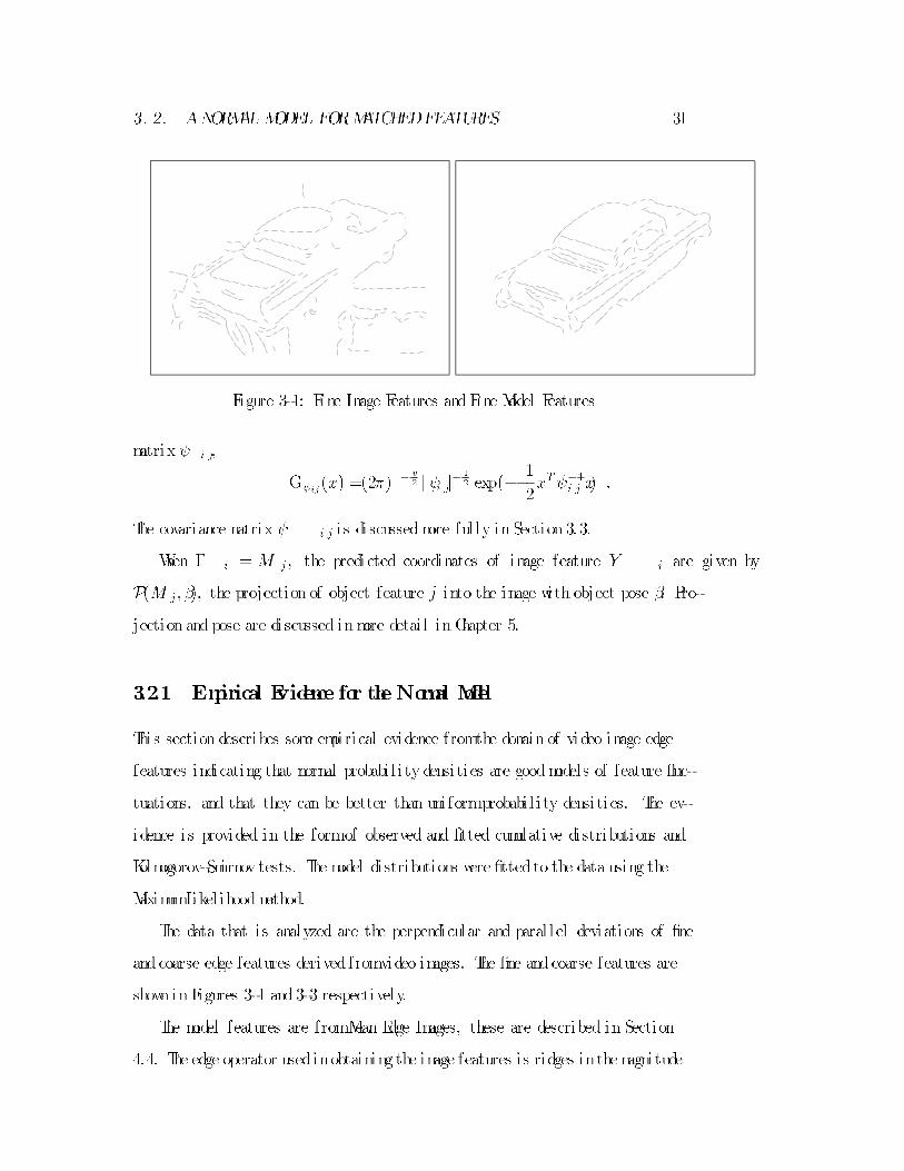
Figure 3-1: Fine Image Features andFine Model Features
matrix i j,
G ij(x) =(2�) �
v2 j i jj�
1
2 exp(� 1
2xT �1i jx) :
The covariance matrix i j i s discussedmore ful ly in Section 3.3.
When � i =M j, the predicted coordinates of image feature Y i are given by
P(M j; �), the projection of object feature j into the image with object pose �. Pro-
jection and pose are discussed inmore detai l in Chapter 5.
3.2.1 Empirical Evidence for theNormal Model
This section describes some empirical evidence fromthe domain of video image edge
features indicating that normal probabi l i tydensities are goodmodels of feature uc-
tuations, and that they can be better than uni formprobabi l i ty densities. The ev-
idence is provided in the formof observed and �tted cumulative distributions and
Kolmogorov-Smirnovtests. The model distributions were �ttedto the data using the
MaximumLikel ihoodmethod.
The data that is analyzed are the perpendicular and paral lel deviations of �ne
andcoarse edge features derivedfromvideo images. The �ne andcoarse features are
shown inFigures 3-1 and 3-3 respectively.
The model features are fromMean Edge Images, these are described in Section
4.4. The edge operator usedinobtaining the image features is ridges inthemagnitude

32 CHAPTER3. MODELI NGIMAGEFEATURES
Figure 3-2: Fine Feature Correspondences
Figure 3-3: Coarse Image Features andCoarse Model Features

3. 2. ANORMAL MODEL FORMATCHEDFEATURES 33
Figure 3-4: Coarse Feature Correspondences

34 CHAPTER3. MODELI NGIMAGEFEATURES
of the image gradient, as discussed inSection4.4. The smoothing standarddeviation
used in the edge detectionwas 2.0 and 4.0 pixels respectively, for the �ne and coarse
features. These features were also used in the experiments reported in Section 10.1,
and the correspondences were used there as training data.
For the analysis in this section, the feature data consists of the average of the
x and y coordinates of the pixels fromedge curve fragments { they are 2Dpoint
features. The features are displayed as circular arc fragments for clari ty. The edge
curves were brokenarbitrari ly into 10 and 20 pixel fragments for the �ne and coarse
features respectively.
Correspondences fromimage features to model features were establ i shed by a
neutral subject using a mouse. These correspondences are indicated by heavy l ines
in Figures 3-2 and 3-4. Perpendicular and paral lel deviations of the corresponding
features were calculated with respect to the normals to edge curves at the image
features.
Figure 3-5 shows the cumulative distributions of the perpendicular and paral lel
deviations of the �ne features. The cumulative distributions of �ttednormal densities
are plottedas heavydots over the observeddistributions. The distributions were�tted
to the data using the MaximumLikel ihoodmethod { the mean and variance of the
normal densityare set to the meanandvariance of the data. These �gures showgood
agreement between the observed distributions, and the �tted normal distributions.
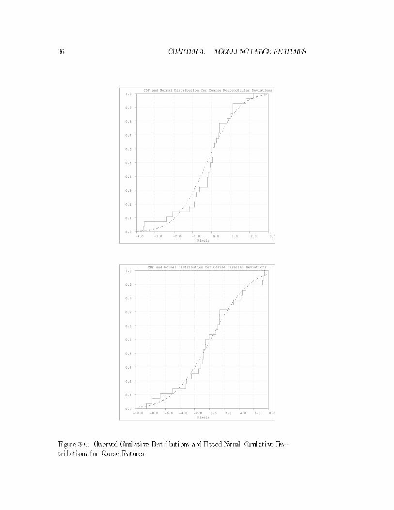
Simi lar observedand�tteddistributions for the coarse deviations are showninFigure
3-6, again with good agreement.
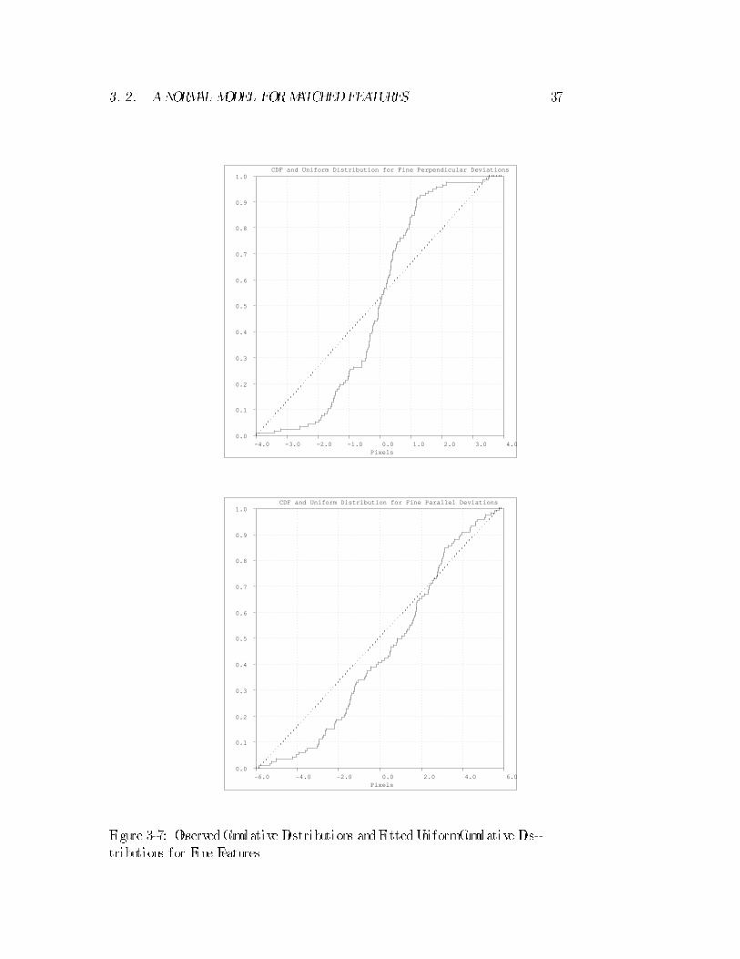
The observed cumulative distributions are shown again in Figures 3-7 and 3-8,
this time with the cumulative distributions of �tted uni formdensities over-plotted
in heavy dots. As before, the uni formdensities were �tted to the data using the
MaximumLikel ihoodmethod{ inthis case the uni formdensities are adjustedto just
include the extreme data. These �gures showrelatively poor agreement between the
observedand�tted distributions, in comparison to normal densities.

3. 2. ANORMAL MODEL FORMATCHEDFEATURES 35
CDF and Normal Distribution for Fine Perpendicular Deviations
-4.0 -3.0 -2.0 -1.0 0.0 1.0 2.0 3.0 4.0Pixels
0.0
0.1
0.2
0.3
0.4
0.5
0.6
0.7
0.8
0.9
1.0
CDF and Normal Distribution for Fine Parallel Deviations
-6.0 -4.0 -2.0 0.0 2.0 4.0 6.0Pixels
0.0
0.1
0.2
0.3
0.4
0.5
0.6
0.7
0.8
0.9
1.0
Figure 3-5: ObservedCumulative Distributions and Fitted Normal Cumulative Dis-
tributions for Fine Features
36 CHAPTER3. MODELI NGIMAGEFEATURES
CDF and Normal Distribution for Coarse Perpendicular Deviations
-4.0 -3.0 -2.0 -1.0 0.0 1.0 2.0 3.0Pixels
0.0
0.1
0.2
0.3
0.4
0.5
0.6
0.7
0.8
0.9
1.0
CDF and Normal Distribution for Coarse Parallel Deviations
-10.0 -8.0 -6.0 -4.0 -2.0 0.0 2.0 4.0 6.0 8.0Pixels
0.0
0.1
0.2
0.3
0.4
0.5
0.6
0.7
0.8
0.9
1.0
Figure 3-6: ObservedCumulative Distributions and Fitted Normal Cumulative Dis-
tributions for Coarse Features
3. 2. ANORMAL MODEL FORMATCHEDFEATURES 37
CDF and Uniform Distribution for Fine Perpendicular Deviations
-4.0 -3.0 -2.0 -1.0 0.0 1.0 2.0 3.0 4.0Pixels
0.0
0.1
0.2
0.3
0.4
0.5
0.6
0.7
0.8
0.9
1.0
CDF and Uniform Distribution for Fine Parallel Deviations
-6.0 -4.0 -2.0 0.0 2.0 4.0 6.0Pixels
0.0
0.1
0.2
0.3
0.4
0.5
0.6
0.7
0.8
0.9
1.0
Figure 3-7: ObservedCumulative Distributions andFittedUni formCumulative Dis-
tributions for Fine Features

38 CHAPTER3. MODELI NGIMAGEFEATURES
CDF and Uniform Distribution for Coarse Perpendicular Deviations
-4.0 -3.0 -2.0 -1.0 0.0 1.0 2.0 3.0Pixels
0.0
0.1
0.2
0.3
0.4
0.5
0.6
0.7
0.8
0.9
1.0
CDF and Uniform Distribution for Coarse Parallel Deviations
-10.0 -8.0 -6.0 -4.0 -2.0 0.0 2.0 4.0 6.0 8.0Pixels
0.0
0.1
0.2
0.3
0.4
0.5
0.6
0.7
0.8
0.9
1.0
Figure 3-8: ObservedCumulative Distributions andFittedUni formCumulative Dis-
tributions for Coarse Features

3. 2. ANORMAL MODEL FORMATCHEDFEATURES 39
Normal Hypothesis Uni formHypothesis
Deviate N Do P (D� D o) Do P(D�D o)
Fine Perpendicular 118 .0824 .3996 .2244 .000014
Fine Paral lel 118 .0771 .4845 .1596 .0049Coarse Perpendicular 28 .1526 .5317 .2518 .0574
Coarse Paral lel 28 .0948 .9628 .1543 .5172
Table 3.1: Kolmogorov-SmirnovTests
Kolmogorov-Smirnov Tests
The Kolmogorov-Smirnov (KS) test [59] i s one way of analyzing the agreement be-
tween observed and �tted cumulative distributions, such as the ones in Figures 3-5
to 3-8. The KS test i s computed on the magnitude of the largest di�erence between
the observed and hypothesized (�tted) distributions. This wi l l be referred to as D.
The probabi l i tydistributiononthis distance, under the hypothesis that the datawere
drawnfromthe hypothesizeddistribution, canbe calculated. Anasymptotic formula
is givenby
P(D�D o) =Q(pNDo)
where
Q(x) =21Xj =1
(�1) j �1exp(�2j 2x
2) ;
andD o i s the observedvalue of D.
The results of KS tests of the consistency of the data with �tted normal and
uni formdistributions are shown in Table 3.1. Lowvalues of P(D�D o) suggest
incompatibi l i ty between the data and the hypothesized distribution. In the cases
of �ne perpendicular and paral lel deviations, and coarse perpendicular deviations,
refutation of the uni formmodel i s strongly indicated. Strong contradictions of the
�tted normal models are not indicated in any of the cases.

40 CHAPTER3. MODELI NGIMAGEFEATURES
3.3 Oriented Stationary Statistics
The covariance matrix i j that appears in the model of matched image features in
Equation 3.2 is al lowed to depend on both the image feature and the object feature
involvedinthe correspondence. Indexing oni al lows dependence onthe image feature
detectionprocess, whi le indexing in j al lows dependence on the identity of the model
feature. This i s useful when some model features are knowto be noisier thanothers.
This exibi l i ty is carriedthroughthe formal ismof later chapters. Althoughsuch ex-
ibi l i ty can be useful , substantial simpl i�cation results by assuming that the features
statistics are stationary in the image, i .e. i j= , for al l ij. This could be reason-
able i f the feature uctuations were isotropic in the image, for example. In its strict
formthis assumptionmay be too l imiting, however. This section outl ines a compro-
mise approach, oriented stationary statistics, that was used in the implementations
described inChapters 6, 7, and 8.
This method involves attaching a coordinate systemto each image feature. The
coordinate systemhas its origin at the point location of the feature, and is oriented
with respect to the direction of the underlying curve at the feature point. When
(stationary) statistics on feature deviations are measured, they are taken relative to
these coordinate systems.
3.3.1 EstimatingtheParameters
The experiments reported inSections 6.2, 7.1, andChapter 10 use the normal model
and oriented stationary statistics for matched image features. After this choice of
model , i t i s sti l l necessary to supply the speci�c parameters for the model , namely,
the covariance matrices, i j, of the normal densities.
The parameters were estimated fromobservations on matches done by hand on
sample images fromthe domain. Because of the stationarityassumption it i s possible
to estimate the common covariance, , by observing match data on one image. For

3. 3. ORI ENTEDSTATIONARYSTATI STI CS 41
this purpose, amatchwas done withamouse betweenfeatures fromaMeanEdge Im-
age (these are described inSection4.4) anda representative image fromthe domain.
During this process, the pose of the object was the same in the two images. This
produced a set of corresponding edge features. For the sake of example, the process
wi l l be described for 2Dpoint features (described inSection5.2). The procedure has
also beenusedwith2Dpoint-radius features and2Doriented-range features, that are
described in Sections 5.3 and 5.4 respectively.
Let the observed image features be described by Y i, and the corresponding mean
model features by Yi. The observedresiduals betweenthe \data" image features, and
the \mean" features are � i =Y i � Yi.
The features are derived fromedge data, and the underlying edge curve has an
orientation angle in the image. These angles are used to de�ne coordinate systems
speci�c to each image feature Y i. These coordinate systems de�ne rotationmatrices
Ri that are usedto transformthe residuals intothe coordinate systems of the features,
in the fol lowing way: � 0
i=R i�i.
The stationary covariance matrix of the matched feature uctuations observed
in the feature coordinate systems is then estimated using the MaximumLikel ihood
method, as fol lows,
=1
n
Xi
�0
i�0 T
i:
Here T denotes the matrix transpose operation. This technique has some bias, but
for the reasonably large sample sizes involved (n� 100) the e�ect is minor.
The resulting covariance matrices typical ly indicate larger variance for deviations
along the edge curve than perpendicular to it, as suggested by the data in Figures
3-5 and 3-6.

42 CHAPTER3. MODELI NGIMAGEFEATURES
3.3.2 SpecializingtheCovariance
At recognitiontime, i t i s necessaryto special ize the constant covariance to eachimage
feature. This i s done by rotating it to orient it with respect to the image feature.
Acovariance matrix transforms l ike the fol lowing product of residuals:
�0
i�0 T
i:
This is transformedback to the image systemas fol lows,
RT
i�0
i�0 T
iRi :
Thus the constant covariance is special izedto the image features inthe fol lowingway,
i j=RT
i R i :

Chapt er 4
Model i ng Object s
What is neededfromobject models? For recognition, the main issue l ies inpredicting
the image features that wi l l appear inanimage of the object. Shouldthe object model
be a monol i thic 3Ddata structure? After al l , the object i tsel f i s 3D. In this chapter,
some pros and cons of monol i thic 3Dmodels are outl ined. An alternative approach,
interpolation of views, i s proposed. The related problemof obtaining the object
model data is discussed, and it i s proposed that the object model data be obtained
by taking pictures of the object. An automatic method for this purpose is described.
Additional ly, a means of edge detection that captures the average edges of anobject
i s described.
4.1 Monol i thic 3D Object Models
One motivation for using 3Dobject models in recognition systems is the observation
that computer graphics techniques can be used to synthesize convincing images from
3Dmodels in any pose desired.
For some objects, havinga single 3Dmodel seems anatural choice for arecognition
system. If the object i s polygonal , andis representedbya l i st of 3Dl ine segments and
vertices, thenpredicting the features that wi l l appear ina givenhigh resolution view
43
44 CHAPTER4. MODELI NGOBJECTS
i s a simple matter. Al l that is needed is to apply a pose dependent transformation to
each feature, and to performa visibi l i ty test.
For other objects, suchas smoothly curvedobjects, the si tuation is di�erent. Pre-
dicting features becomes more elaborate. Invideo imagery, occluding edges (or l imbs)
are often important features. Calculating the l imbof a smooth 3Dsurface is usual ly
compl icated. Ponce and Kriegman [58] describe an approach for objects modeled
by parametric surface patches. Algebraic el imination theory is used to relate image
l imbs to the model surfaces that generated them. Brooks' vision system, Acronym
[10] , also recognized curved objects fromimage l imbs. It used general ized cyl inders
to model objects. Adrawback of this approach is that it i s awkward to real i stical ly
model ing typical objects, l ike telephones or automobi les, with general ized cyl inders.
Predicting reduced resolution image features is another di�cultywithmonol i thic
3Dmodels. This i s a drawback because doing recognition with reduced resolution
features is anattractive strategy: with fewer features less searchwi l l be needed. One
solution would be to devise a way of smoothing 3Dobject models such that simple
projection operations would accurately predict reduced resolution edge features. No
suchmethod is known to the author.
Detecting reduced resolution image features is straightforward. Good edge fea-
tures of this sort may be obtained by smoothing the grayscale image before using an
edge operator. This method is commonly used with the Canny edge operator [13] ,
andwith the Marr-Hi ldreth operator [53] .
Analternative approachis to doprojections of the object model at ful l resolution,
and then to do some kind of smoothing of the image. It i sn't clear what sort of
smoothing wouldbe needed. One possibi l i ty is to do photometrical ly real i stic projec-
tions (for example by ray tracing rendering), performsmoothing in the image, and
then use the same feature detection scheme as is used on the images presented for
recognition. This methodis l ikelyto be tooexpensive for practical recognitionsystem
that need to performlarge amounts of prediction. Perhaps better ways of doing this

4. 2. I NTERPOLATIONOF VI EWS 45
wi l l be found.
Sel f occlusion is an additional complexity of the monol i thic 3Dmodel approach.
In computer graphics there are several ways of deal ing with this i ssue, among them
hidden l ine and z-bu�er methods. These methods are fairly expensive, at least in
comparison to sparse point projections.
In summary, monol i thic 3Dobject models address some of the requirements for
predicting images for recognition, but the computational cost may be high.
4.2 Interpolation of Views
One approachto avoiding the di�culties discussed inthe previous section is to use an
image-basedapproachto object model ing. Ul lmanandBasri [71] have discussedsuch
approaches. There is some biological evidence that animal visionsystems have recog-
nition subsystems that are attuned to speci�c views of faces [25] . This may provide
some assurance that image-based approaches to recognition aren't unreasonable.
An important issue with image-based object model ing concerns howto predict
image features in a way that covers the space of poses that the object may assume.
Bodies undergoing rigid motion in space have six degrees of freedom, three in
translation, andthree inrotation. This sixparameter pose spacemaybe spl i t intotwo
parts { the �rst part being translationandinimage-plane rotations (four parameters)
{ the second part being out of image-plane rotations (two parameters: the \view
sphere").
Synthesizing views of an object that span the �rst part of pose space can often
be done using simple and e�cient l inear methods of translation, rotation, and scale
in the plane. This approach can be precise under orthographic projection with scal -
ing, and accurate enough in some domains with perspective projection. Perspective
projection is often approximated in recognition systems by 3Drotation combined
with orthographic projection and scal ing. This has been cal led the weak perspect i ve

46 CHAPTER4. MODELI NGOBJECTS
approximation [70] .
The second part of pose space, out of plane rotation, i s more compl icated. The
approach advocated in this research involves tesselating the viewsphere around the
object, and storing a viewof the object for each vertex of the tesselation. Arbitrary
views wi l l thenentai l , at most, smal l out of plane rotations fromstoredviews. These
views may be synthesized using interpolation. The Linear Combination of Views
method of Ul lman andBasri [71] , works wel l for interpolating betweennearby views
(andmore distant ones, as wel l ).
Conceptual ly, the interpolationof views methodcaches pre-computedpredictions
of images, saving the expense of repeatedly computing themduring recognition. If
the tesselation is dense enough, di�culties owing to large changes in aspect may be
avoided.
Breuel [9] advocates a view-based approach to model ing, without interpolation.
4.3 Object Models fromObservation
Howcan object model features be acquired for use in the interpolation of views
framework? If a detai led CADmodel of the object i s avai lable, then views might be
synthesizedusinggraphical rendering programs (this approachwas usedinthe (single
view) laser radar experiment described in Section 7.3).
Another method is to use the object i tsel f as i ts ownmodel , and to acquire views
by taking pictures of the object. This process canmake use of the feature extraction
method that is used on images at recognition time. An advantage of this scheme is
that anaccurate CADstylemodel i sn't needed. Using the run-time feature extraction
mechanismof the recognition systemautomatical ly selects the features that wi l l be
sal ient at recognition time, which is otherwise a potential ly di�cult problem.
One di�culty with the models fromobservation approach is that image features
tendtobe somewhat unstable. For example, the presence andlocationof edge features
4. 4. MEANEDGE IMAGES 47
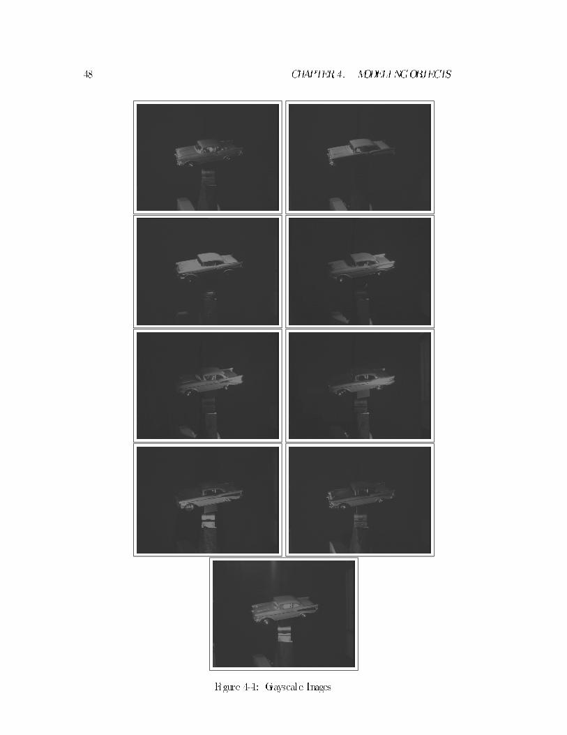
is in uencedby i l luminationconditions, as i l lustrated inthe fol lowing �gures. Figure
4-1 shows a series of nine grayscale images where the only variation is in l ighting. A
corresponding set of edge images is shownin4-2. The edge operator usedinpreparing
the images is described in Section 4.4. The standard deviation of the smoothing
operator was 2 pixels.
4.4 MeanEdge Images
It was pointedout above that the instabi l i ty of edge features is a potential di�culty
of acquiring object model features fromobservation. The MeanEdge Image method
solves this problemby making edge maps that are averaged over variations due to
i l lumination changes.
Brightness edges may be characterized as the ridges of a measure of brightness
variation. This i s consistent with the common notion that edges are the 1Dloci of
maxima of changes inbrightness. The edge operator used inFigure 4-2 is anexample
of this style of edge detector. It i s a ridge operator appl ied to the squared discrete
gradient of smoothed images. Here, the squared discrete gradient is the measure of
brightness variation. This style of edge detectionwas described byMercer [57] . The
mathematical de�nitionof the ridge predicate is that the gradient is perpendicular to
the directionhaving the most negative seconddirectional derivative. Another simi lar
de�nitionof edges was proposedHaral ick [37] . For a general surveyof edge detection
methods, see Robot Vi si on, byHorn [39] .
The precedingcharacterizationof image edges general izes natural lytomeanedges.
Meanedges are de�nedto be ridges in the average measure of brightness uctuation.
In this work, average brightness uctuation over a set of pictures is obtained by
averaging the squared discrete gradient of the (smoothed) images.
Figure 4-3 shows the averagedsquaredgradient of smoothedversions of the images
that appear inFigure 4-1. Recal l that onlythe l ightingchangedbetweenthese images.
48 CHAPTER4. MODELI NGOBJECTS
Figure 4-1: Grayscale Images

4. 4. MEANEDGE IMAGES 49
Figure 4-2: Edge Images

50 CHAPTER4. MODELI NGOBJECTS
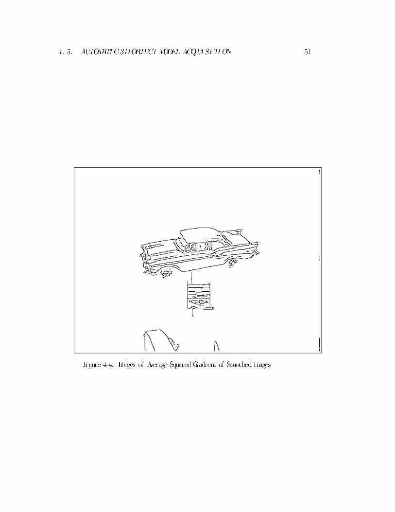
Figure 4-3: AveragedSquaredGradient of Smoothed Images
Figure 4-4 shows the ridges fromthe image of Figure 4-3. Hysteresi s thresholding
based on the magnitude of the averaged squared gradient has been used to suppress
weakedges. Suchhysteresi s thresholding is usedwiththe Cannyedge operator. Note
that this edge image is relatively immune to specular highl ights, incomparisonto the
individual edge images of Figure 4-4.
4.5 Automatic 3DObject Model Acquisi tion
This section outl ines a method for automatic 3Dobject model acquisi tion that com-
bines interpolationof views andMeanEdge Images. The method involves automati -
cal ly acquiring (many) pictures of the object under various combinations of pose and
i l lumination. Aprel iminary implementationof themethodwas usedto acquire object
model features for the 3Drecognition experiment discussed in Section 10.4.
4. 5. AUTOMATI C3DOBJECTMODEL ACQUI SI TI ON 51
Figure 4-4: Ridges of Average SquaredGradient of Smoothed Images

52 CHAPTER4. MODELI NGOBJECTS
Figure 4-5: APentakis Dodecahedron
The object, a plastic car model , was mounted on the tool ange of a PUMA560
robot. Avideo camera connected to a Sun Microsystems VFCvideo digitizer was
mountednear the robot.
For the purpose of Interpolation of Views object model construction, the view
sphere aroundthe object was tesselated into32 viewpoints, the vertices of a pentakis
dodecahedron(one is i l lustratedinFigure 4-5). At eachviewpoint a\canonical pose"
for the object was constructedthat orientedthe viewpoint towards the camera, whi le
keeping the center of the object in a �xed position.
Nine di�erent con�gurations of l ighting were arranged for the purpose of con-
structing Mean Edge Images. The l ighting con�gurations were made by moving a
spotl ight to nine di�erent position that i l luminated the object. The lamp positions
roughly covered the viewhemisphere centeredon the camera.
The object was moved to the canonical poses corresponding to the 21 vertices in

4. 5. AUTOMATI C3DOBJECTMODEL ACQUI SI TI ON 53
the upper part (roughly 2/3) of the object' s viewsphere. At each of these poses,
pictures were takenwith eachof the nine lamppositions.
Mean Edge Images at various scales of smoothing were constructed for each of
the canonical poses. Object model features for recognition experiments described in
Chapter 8 were derived fromthese Mean Edge Images. Twenty of the images from
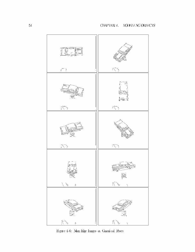
one such set of MeanEdge Images are displayed in Figures 4-6 and 4-7.
Two of these Mean Edge Images were used in an experiment in 3Drecognition
using a two-viewLinear Combinationof Views method. This method requires corre-
spondences amongfeatures at di�eringviews. These correspondences were establ i shed
by hand, using a mouse.
It i s l ikely that such feature correspondence could be derived fromthe results
of a motion program. Shashua's motion program[65] , which combines geometry
and optical ow, was tested on images fromthe experimental setup and was able
to establ i sh good correspondences at the pixel level , for views separated by 4.75
degrees. This range could be increased by a sequential bootstrapping process. If
correspondences canbe automatical ly determined, thenthe entire process of bui lding
view-basedmodels for 3Dobjects can be made ful ly automatic.
After performing the experiments reportedinChapter 10, i t became apparent that
the views were separatedby too large of anangle (about 38 degrees) for establ i shing
a goodamount of feature correspondence betweensome views. This problemmaybe
rel ievedbyusingmore views. Usingmore views also makes automatic determination
of correspondences easier. If the process of model construction is ful ly automatic,
having a relatively large number of views is potential lyworkable.
The work of Taylor and Reeves [69] provides some evidence for the feasibi l i ty of
multiple-view-based recognition. They describe a classi�cation-based vision system
that uses a l ibrary of views froma 252 vertex icosahedron-based tesselation of the
viewsphere. Their views were separated by 6.0 to 8.7 degrees. They report good
classi�cation of aircraft si lhouettes using this approach.
54 CHAPTER4. MODELI NGOBJECTS
Figure 4-6: MeanEdge Images at Canonical Poses

4. 5. AUTOMATI C3DOBJECTMODEL ACQUI SI TI ON 55
Figure 4-7: MeanEdge Images at Canonical Poses

56 CHAPTER4. MODELI NGOBJECTS
Chapt er 5
Model i ng Proj ect i on
This chapter is concernedwith the representations of image andobject features, and
with the projection of object features into the image, given the pose of the object.
Four di�erent formulations are described, three of which are used in experiments
reported in other chapters.
The �rst three models described in this chapter are essential ly 2D, the trans-
formations comprise translation, rotation, and scal ing in the plane. Such methods
may be used for single views of 3Dobjects via the weak perspective approximation,
as described in [70] . In this scheme, perspective projection is approximated by or-
thographic projection with scal ing. Within this approximation, these methods can
handle four of the six parameters of rigid bodymotion { everything but out of plane
rotations.
The method described in Section 5.5, i s based on Linear Combination of Views,
a view-based 3Dmethod that was developed byUl lman andBasri [71] .
5.1 Linear ProjectionModels
Pose determination is often a component of model -based object recognition systems,
includingthe systems describedinthis thesis. Posedeterminationis frequentlyframed
57
58 CHAPTER5. MODELI NGPROJECTION
as an optimization problem. The pose determination problemmay be signi�cantly
simpl i�ed i f the feature projectionmodel i s l inear inthe pose vector. The systems de-
scribed in this thesis use projectionmodels having this property, this enables solving
the embedded optimization problemusing least squares. Least squares is advanta-
geous because unique solutions may be obtained easi ly in closed form. This i s a
signi�cant advantage, since the embeddedoptimizationproblemis solvedmanytimes
during the course of a search for an object in a scene.
Al l of the formulations of projectiondescribedbeloware l inear in the parameters
of the transformation. Because of this theymay be written in the fol lowing form:
�i =P(M i; �) =M i� : (5:1)
The pose of the object i s represented by �, a column vector, the object model
feature byM i, a matrix. � i, the projection of the model feature into the image by
pose �, i s a columnvector.
Although this particular formmay seemodd, i t a natural one i f the focus is on
solving for the pose and the object model features are constants.
5.2 2DPoint Feature Model
The �rst, and simplest, method to be describedwas usedbyFaugeras andAyache in
their vision systemHYPER[1] . It i s de�ned as fol lows: � i =M i�, where
�i =
264 p0
i x
p0
i y
375 Mi =
264 pi x �p i y 1 0
pi y pi x 0 1
375 and �=
2666666664
�
�
tx
ty
3777777775:
The coordinates of object model point i are p i x and p i y. The coordinates of the

5. 3. 2DPOI NT-RADI US FEATUREMODEL 59
model point i, projectedintothe image bypose �, are p 0
i xandp 0
i y. This transformation
is equivalent to rotation by �, scal ing by s, and translation byT, where
T=
264 tx
ty
375 s=q�2 +� 2
�=arctan
�
�
!:
This representation has an un-symmetrical way of representing the two classes
of features, which seems odd due to their essential equivalence, however the trick
faci l i tates the l inear formulation of projection given inEquation 5.1.
In this model , rotation and scale are e�ected by analogy to the multipl ication of
complexnumbers, whichinduces transformations of rotationandscale inthe complex
plane. This analogy may be made complete by noting that the algebra of complex
numbers a+ib i s i somorphic with that of matrices of the form
264 a b
�b a
375.
5.3 2DPoint-Radius Feature Model
This section describes an extension of the previous feature model that incorporates
informationabout the normal andcurvature at a point ona curve (inadditionto the
coordinate information).
There are advantages in using richer features in recognition { they provide more
constraints, and can lead to space and time e�ciencies. These potential advantages
must be weighedagainst the practical i tyof detecting the richer features. For example,
there is incentive to construct features incorporating higher derivative informationat
apoint onacurve; however, measuringhigher derivatives of curves derivedfromvideo
imagery is probably impractical , because eachderivative magni�es the noise present

60 CHAPTER5. MODELI NGPROJECTION
P
Ci
i
Figure 5-1: Edge Curve, Osculating Circle, andRadius Vector
in the data.
The feature describedhere is a compromise betweenrichness anddetectabi l i ty. It
i s de�ned as fol lows � i =M i�, where
�i =
2666666664
p0
i x
p0
i y
c0
i x
c0
i y
3777777775Mi =
2666666664
pi x �p i y 1 0
pi y pi x 0 1
ci x �c i y 0 0
ci y ci x 0 0
3777777775and �=
2666666664
�
�
tx
ty
3777777775:
The point coordinates and�are as above. c i x and c i y represent the radius vector
of the curve's osculating circle that touches the point on the curve, as i l lustrated
in Figure 5-1. This vector is normal to the curve. Its length is the inverse of the
curvature at the point. The counterparts in the image are givenby c 0
i xand c 0
i y. With
this model , the radius vector c rotates and scales as do the coordinates p, but it does
not translate. Thus, the aggregate feature translates, rotates and scales correctly.
This feature model i s used in the experiments described in Sections 6.2, 7.4, and
5. 4. 2DORI ENTED- RANGEFEATUREMODEL 61
10.1 When the underlying curvature goes to zero, the length of the radius vector
diverges, and the direction becomes unstable. This has been accommodated in the
experiments by truncating c. Although this violates the \transforms correctly" cri te-
rion, the model sti l l works wel l .
5.4 2DOriented-Range Feature Model
This feature projectionmodel i s very simi lar to the one described previously. It was
designedfor use inrange imagery insteadof video imagery. Like the previous feature,
i t i s �tted to fragments of image edge curves. In this case, the edges label discon-
tinuities in range. It i s de�ned just as above in Section 5.3, but the interpretation
of c i s di�erent. The point coordinates and � are as above. As above, c i x and c i y
are a vector whose direction is perpendicular to the (range discontinuity) curve frag-
ment. The di�erence is that rather than encoding the inverse of the curvature, the
lengthof the vector encodes insteadthe inverse of the range at the discontinuity. The
counterparts in the image are given by c 0
i xand c 0
i y. The aggregate feature translates,
rotates andscales correctlywhenusedwithimagingmodels where the object features
scale according to the inverse of the distance to the object. This holds under per-
spective projectionwith attached range labels when the object i s smal l compared to
the distance to the object.
This model was used in the experiments described in Section 7.3.
5.5 Linear Combinationof Views
The technique used inthe abovemethods for synthesizing rotationandscale amounts
to making l inear combinations of the object model with a copy of i t that has been
rotated 90 degrees in the plane.
In their paper, \RecognitionbyLinear Combinationof Models" [71] , Ul lman and
Basri describe a scheme for synthesizing views under 3Dorthography with rotation

62 CHAPTER5. MODELI NGPROJECTION
and scale that has a l inear parameterization. They showthat the space of images of
an object i s a subspace of a l inear space that is spannedby the components of a few
images of anobject. Theydiscuss variants of their formulationthat are basedontwo
views, and on three andmore views. Recovering conventional pose parameters from
the l inear combination coe�cients is described in [60] .
The fol lowingis abrief explanationof the two-viewmethod. The reader is referred
to [71] for a ful ler description. Point projectionfrom3Dto 2Dunder orthography, ro-
tation, andscale i s a l inear transformation. If two(2D) views are avai lable, alongwith
the transformations that produced them(as in stereo vision), then there is enough
data to invert the transformations and solve for the 3Dcoordinates (three equations
are needed, four are avai lable). The resulting expression for the 3Dcoordinates wi l l
be a l inear equation in the components of the two views. New2Dviews may then
be synthesized fromthe 3Dcoordinates by yet another l inear transformation. Com-
pounding these l inear operations yields anexpression for new2Dviews that is l inear
in the components of the original two views. There is a quadratic constraint on the
3Dto2Dtransformations, due to the constraints onrotationmatrices. The usual Lin-
ear Combination of Views approachmakes use of the above l inearity property whi le
synthesizing newviews withgeneral l inear transformations (without the constraints).
This practice leads to two extra parameters that control stretching transformations
in the synthesized image. It also reduces the need to deal with camera cal ibrations {
the pixel aspect ratio may be accommodated in the stretching transformations.
The fol lowingprojectionmodel uses a twoviewvariant of the Linear Combination
of Views methodto synthesize views withl imited3Drotationandscale. Additional ly,
translation has been added in a straightforwardway. � i =M i�, where
�i =
264 �i x
�i y
375 Mi =
264 pi x 0 q i x 0 p i y 0 1 0
0 p i y 0 q i y 0 p i x 0 1
375

5. 5. LI NEARCOMBINATIONOF VI EWS 63
and
�=
��0�1�2�3�4�5�6�7
�T
:
The coordinates of the i ' th point in one vieware p i x and p i y; in the other view
they are q i x and q i y.
When this projectionmodel i s used, �does not in general describe rigid transfor-
mation, but it i s nevertheless cal led the pose vector for notational consistency.
This method is used in the experiment described in Section 10.4.

64 CHAPTER5. MODELI NGPROJECTION
Chapt er 6
MAPModel Mat chi ng
MAPModel Matching 1 (MMM) is the �rst of two statistical formulations of object
recognition to be discussed in this thesis. It bui lds on the models of features and
correspondences, objects, andprojection that are described in the previous chapters.
MMMevaluates joint hypotheses of matchandpose in terms of their posterior prob-
abi l i ty, given an image. MMMis the starting point for the second formulation of
object recognition, Posterior Marginal Pose Estimation (PMPE), which is described
inChapter 7.
The MMMobjective function is amenable to search in correspondence space,
the space of al l possible assignments fromimage features to model and background
features. This style of search has been used in many recognition systems, and it i s
used here in a recognition experiment involving lowresolution edge features.
It i s shown that under certain conditions, searching in pose space for maxima of
the MMMobjective function is equivalent to robust methods of chamfer matching
[47] .
1Early versions of thi s work appeared in [74] and [75] .
65

66 CHAPTER6. MAPMODEL MATCHING
6.1 Objective Function for Pose and Correspon-
dences
In this section an objective function for evaluating joint hypotheses of match and
pose using the MAPcriterion wi l l be derived.
Brie y, probabi l i ty densities of image features, conditioned on the parameters of
match and pose (\the parameters"), are combined with prior probabi l i ties on the
parameters using Bayes' rule. The result i s a posterior probabi l i tydensity on the pa-
rameters, givenanobservedimage. Anestimate of the parameters i s thenformulated
by choosing themso as to maximize their a-posteriori probabi l i ty. (Hence the term
MAP. See BeckandArnold's textbook [4] for a discussionof MAPestimation.) MAP
estimators are especial ly practical when usedwith normal probabi l i ty densities.
This research focuses on feature based recognition. The probabi l i stic models of
image features described inChapter 3 are used. Initial ly, image features are assumed
to be mutual ly independent (this i s relaxed in Section 6.1.1). Additional ly, matched
image features are assumedtobe normal lydistributedabout their predictedpositions
in the image, and unmatched (background) features are assumed to be uni formly
distributed in the image. These densities are combined with a prior model of the
parameters. When a l inear projectionmodel i s used, a simple objective function for
matchandpose results.
As described in Chapter 2, the image that is to be analyzed is represented by a
set of v-dimensional columnvectors.
Y=fY 1; Y2; : : : ; Yng ; Yi 2R v:
The object model i s denoted byM,
M=fM 1;M2; : : : ;Mmg :
6. 1. OBJECTI VE FUNCTIONFORPOSE ANDCORRESPONDENCES 67
Whenl inear projectionmodels are used, as discussedinChapter 5, the object features
wi l l be representedby real matrices: M j 2R v�z (z i s de�nedbelow).
The parameters to be estimated in matching are the correspondences between
image and object features, and the pose of the object in the image. As discussed in
Section 2.1, the state of match, or correspondences, i s described by the variable �:
�=f� 1;�2; : : : ;�ng ; �i 2M[f?g :
Here � i =M j means that image feature i corresponds to object model feature j, and
�i =?means that image feature i i s due to the background.
The pose of the object i s a real vector: �2R z. Aprojection function, P(), maps
object model features into the v-dimensional image coordinate space according to the
pose,
P(M i; �) 2R v:
The probabi l i stic models of image features described inChapter 3maybe written
as fol lows:
p(Y i j �; �) =
8><>:1
W1W2�� � Wvi f �i =?
G ij(Yi �P(M j; �)) i f � i =M j
(6:1)
where
G ij(x) =(2�) �
v2 j ij�
1
2 exp(� 1
2x
T
�1ix) :
Here i j i s the covariancematrixassociatedwithimage feature i andobject model
feature j. Thus image features arising fromthe backgroundare uni formlydistributed
over the image feature coordinate space (the extent of the image feature coordinate
space along dimension i i s given byW i), and matched image features are normal ly
distributedabout their predictedlocations inthe image. Insome appl ications could
be independent i f i and j { an assumption that the feature statistics are stationary
in the image, or may depend only on i, the image feature index. The latter i s the
case when the oriented stationary statistics model i s used (see Section 3.3).

68 CHAPTER6. MAPMODEL MATCHING
Assuming independent features, the joint probabi l i ty density on image feature
coordinates may be written as fol lows
p(Y j �; �) =Yi
p(Y i j �; �) =Y
i :�i=?
1
W1W2 � � � WvY
i j : �i=M j
G ij(Yi �P(M j; �)) :
(6:2)
This assumption often holds when sensor noise dominates in feature uctuations.
The next step in the derivation is the construction of a joint prior on correspon-
dences andpose. InChapter 2, probabi l i stic models of feature correspondences were
discussed. The independent correspondence model i s used here for simpl ici ty. Use of
the Markov correspondence model i s discussed in the fol lowing section. The proba-
bi l i tythat image feature i belongs to the backgroundis B i, whi le the remainingprob-
abi l i ty is uni formly distributed for correspondences to the m object model features.
In some situations, B i maybe a constant, independent of i. Recal l ing Equations 2.1
and 2.6,
p(�) =Yi
p(� i) and p(� i) =
8><>: Bi i f �i =?1�Bi
motherwise :
(6:3)
Prior information on the pose is assumed to be suppl ied as a normal density,
p(�) =G �(��� 0)
where
G �(x) =(2�)
�z2 j �j�
1
2 exp(� 1
2x
T
�1�x) :
Here � i s the covariance matrix of the pose prior and z i s the dimensional i ty of
the pose vector, �. With the combinationof normal pose priors and l inear projection
models the systemis closed in the sense that the resulting pose estimate wi l l al so
be normal . This i s convenient for coarse-�ne, as discussed in Section 6.4. If l i ttle i s
knownabout the pose a-priori , the prior maybe made quite broad. This i s expected
to be often the case. If nothing is knownabout the pose beforehand, the pose prior
6. 1. OBJECTI VE FUNCTIONFORPOSE ANDCORRESPONDENCES 69
maybe left out. In that case the resulting cri terion for evaluating hypotheses wi l l be
based onMaximumLikel ihood for pose, and onMAPfor correspondences.
Assuming independence of the correspondences and the pose (before the image is
compared to the object model), a mixed joint probabi l i ty functionmaybe writtenas
fol lows,
p(�; �) =G �(��� 0)
Yi : �i=?
Bi
Yi : �i 6=?
1�B i
m
:
This a good assumption when view-based approaches to object model ing are used
(these are discussed in Chapter 4 and used in the experiments described in Chapter
10). (With general 3Drotation it i s inaccurate, as the visibi l i ty of features depends
onthe orientationof the object. ) This probabi l i ty functiononmatchandpose is now
usedwith Bayes' rule as a prior for obtaining the posterior probabi l i ty of �and�:
p(�; �j Y) = p(Y j �; �)p(�; �)p(Y)
; (6:4)
where p(Y) =P
�
Rd� p(Y j �; �)p(�; �) i s a normal ization factor that is formal ly
the probabi l i tyof the image. It i s a constant withrespect to �and�, the parameters
being estimated.
The MAPstrategy is used to obtain estimates of the correspondences and pose
bymaximizing their posterior probabi l i tywith respect to �and �, as fol lows
d�; �=argmax�;�
p(�; �j Y) :
For convenience, anobjective function, L, i s introduced that is a scaled logarithm
of p(�; �j Y). The same estimates wi l l result i f the maximization is instead carried
out over L. d�; �=argmax�; �
L(�; �)
where
L(�; �) �ln p(�; �j Y)
C
!: (6:5)
70 CHAPTER6. MAPMODEL MATCHING
The denominator in Equation 6.5 is a constant that has been chosen to cancel con-
stants fromthe numerator. Its value, which is independent of �and � i s
C=B1B2 � � � Bn
(W1W2 � � � Wv)n(2�)
�z2 j �j
�1
2
1
p(Y):
After some manipulation the objective functionmay be expressed as
L(�; �) =� 1
2(��� o)
T �1�(��� 0)+
Xi j : �i=M j
[�i j�1
2(Yi�P(M j; �))
T �1i j(Yi�P(M j; �))]
(6:6)
, where
�i j=ln
1
(2�)v2m
(1�B i)
Bi
W1W2 � � � Wvj i jj
1
2
!: (6:7)
When a l inear projection model i s used, P(M j; �) =M j�. (Linear projection
models were discussed in Chapter 5.) In this case, the objective function takes the
fol lowing simple form
L(�; �) =� 1
2(��� o)
T
�1�(��� 0)+
Xi j : �i=M j
[�i j�1
2(Yi�M j�)
T
�1i j(Yi�M j�)] : (6:8)
When the background probabi l i ty is constant, and when the feature covariance
matrix determinant is constant (as when oriented stationary statistics are used), the
formulas simpl i fy further {
�=ln
1
(2�)v2m
(1�B)B
W1W2 � � � Wvj j 1
2
!; (6:9)
and
L(�; �) =� 1
2(��� o)
T �1�(��� 0)+
Xi j : �i=M j
[�� 1
2(Yi�M j�)
T �1i(Yi�M j�)] : (6:10)
Here, i s the stationary feature covariance matrix, and i i s the special ized
feature covariance matrix. These were discussed in Section 3.3.

6. 1. OBJECTI VE FUNCTIONFORPOSE ANDCORRESPONDENCES 71
The �rst termof the objective function of Equation 6.8 expresses the in uence of
the prior on the pose. As discussed above, when a useful pose prior i sn't avai lable,
this termmaybe dropped.
The second termhas a simple interpretation. It i s a sumtaken over those image
features that are matched to object model features. The � i j are �xed rewards for
making correspondences, whi le the quadratic forms are penalties for deviations of ob-
served image features fromtheir expectedpositions in the image. Thus the objective
function evaluates the amount of the image explained in terms of the object, with
penalties for mismatch. This objective function is particularly simple in terms of �.
When�is constant, �and its (posterior) covariance are estimatedbyweighted least
squares. When using an algorithmbased on search in correspondence space, the es-
timate of �can be cheaply updated by using the techniques of sequential parameter
estimation. (See BeckandArnold [4] . ) The � i j describe the relative value of amatch
component or extension in a way that al lows direct comparison to the entai ledmis-
matchpenalty. The values of these trade-o�parameter(s) are suppl ied by the theory
(inEquation 6.7) and are given in terms of measurable domain statistics.
The formof the objective function suggests an optimization strategy: make cor-
respondences to object features inorder to accumulate correspondence rewards whi le
avoiding penalties for mismatch. It i s important that the � i j be positive, otherwise a
winning strategy is be tomake nomatches to the object at al l . This conditionde�nes
a cri tical level of image clutter, beyondwhichthe MAPcriteria assigns the feature to
the background. � i j describes the dependence of the value of matches on the amount
of background clutter. If background features are scarce, then correspondences to
object features become more important.
This objective function provides a simple and uni formway to evaluate match
and pose hypotheses. It captures important aspects of recognition: the amount of
image explained in terms of the object, as wel l as the metrical consistency of the
hypothesis; and it trades themo�ina rational waybasedondomainstatistics. Most
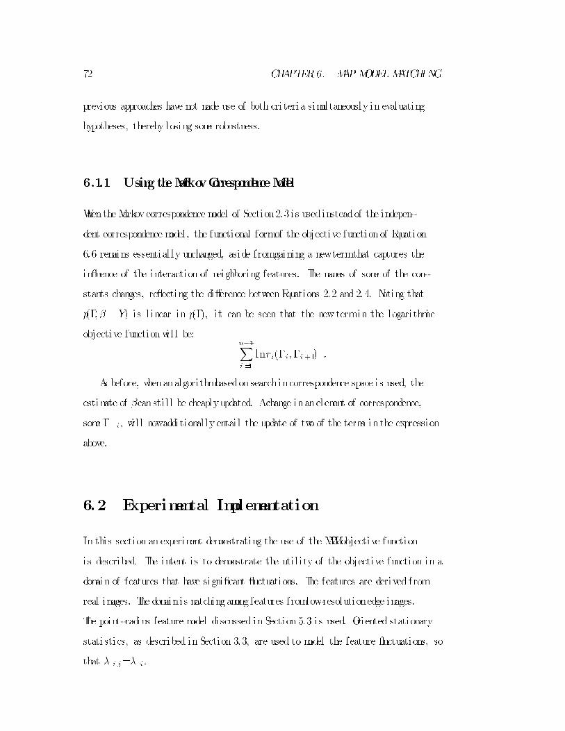
72 CHAPTER6. MAPMODEL MATCHING
previous approaches have not made use of both criteria simultaneously in evaluating
hypotheses, thereby losing some robustness.
6.1.1 UsingtheMarkovCorrespondenceModel
Whenthe Markovcorrespondence model of Section2.3 is usedinsteadof the indepen-
dent correspondence model , the functional formof the objective functionof Equation
6.6 remains essential ly unchanged, aside fromgaining a newtermthat captures the
in uence of the interaction of neighboring features. The names of some of the con-
stants changes, re ecting the di�erence betweenEquations 2.2 and 2.4. Noting that
p(�; � j Y) i s l inear in p(�), i t can be seen that the newtermin the logarithmic
objective functionwi l l be:n�1Xi =1
lnri(�i;�i +1) :
As before, whenanalgorithmbasedonsearchincorrespondence space is used, the
estimate of �cansti l l be cheaplyupdated. Achange inanelement of correspondence,
some � i, wi l l nowadditional ly entai l the update of two of the terms inthe expression
above.
6.2 Experimental Implementation
In this section an experiment demonstrating the use of the MMMobjective function
is described. The intent is to demonstrate the uti l i ty of the objective function in a
domain of features that have signi�cant uctuations. The features are derived from
real images. The domainis matchingamongfeatures fromlow-resolutionedge images.
The point-radius feature model discussed in Section 5.3 is used. Oriented stationary
statistics, as described in Section 3.3, are used to model the feature uctuations, so
that � i j=� i.

6. 2. EXPERIMENTAL IMPLEMENTATION 73
6.2.1 SearchinCorrespondenceSpace
Good solutions of the objective function of Equation 6.8 are sought by a search in
correspondence space. Searchover the whole exponential space is avoidedbyheuristic
pruning.
Anobjective functionthat evaluates a con�gurationof correspondences, or match
(described by �), may be obtained as fol lows:
L(�) =max�
L(�; �) :
This optimization is quadratic in�andis carriedout by least squares. Sequential
techniques are used so that the cost of extending a partial match by one correspon-
dence is O(1) .
The space of correspondences maybe organizedas adirected-acycl ic-graph(DAG)
by the fol lowing parent-chi ld relation onmatches. Apoint in correspondence space,
or match i s a chi ldof another match i f there is some i suchthat � i =?in the parent,
and � i =M j , for some j, in the chi ld, and they are otherwise the same. Thus, the
chi ldhas onemore assignment to themodel thanthe parent does. This DAGis rooted
in the matchwhere al l assignments are to the background. Al l possible matches are
reachable fromthe root. Afragment of an example DAGof this kind is i l lustrated
inFigure 6-1. Components of matches that are not expl ici t in the �gure are assigned
to the background.
Heuristic beamsearch, as describedin[64] , i s usedto searchover matches for good
solutions of L. Success depends on the heuristic that there aren't many impostors in
the image. An impostor is a set of image features that scores wel l but isn't a subset
of the optimummatch impl iedby the objective function. Another wayof stating the
heuristic i s that the best match to n+1 object features is l ikely to contain the best
match to nobject features.
The searchmethod used in the experiments employs a bootstrapping mechanism
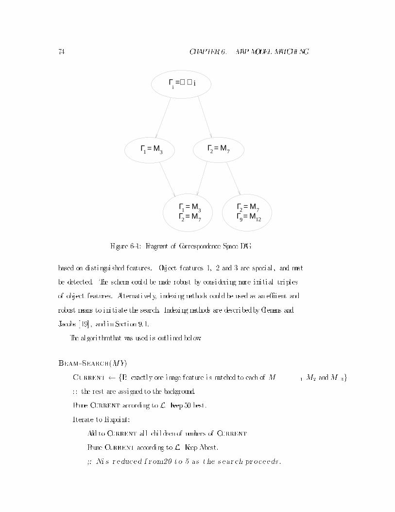
74 CHAPTER6. MAPMODEL MATCHING
Γ =⊥ ∀i
i
Γ = Μ 1 3Γ = Μ 2 7Γ = Μ 9 12
Γ = Μ 1 3Γ = Μ 2 7
Γ = Μ 2 7
Figure 6-1: Fragment of Correspondence Space DAG
based on distinguished features. Object features 1, 2 and 3 are special , and must
be detected. The scheme could be made robust by considering more initial triples
of object features. Alternatively, indexing methods could be used as an e�cient and
robust means to initiate the search. Indexingmethods are describedbyClemens and
Jacobs [19] , and in Section 9.1.
The algorithmthat was used is outl ined below.
Beam-Search(M, Y)
Current f�: exactly one image feature is matched to each of M 1 M2 andM 3g
; ; the rest are assigned to the background.
Prune Current according to L. Keep 50 best.
Iterate to Fixpoint:
Add toCurrent al l chi ldrenof members of Current
Prune Current according to L. KeepNbest.
;; Ni s r educed f r om20 t o 5 as t he s ear ch pr oceeds .

6. 2. EXPERIMENTAL IMPLEMENTATION 75
Figure 6-2: Images used for Matching
Return(Current)
Sometimes an extension of a match wi l l produce one that is already in Cur-
rent, that was reached in a di�erent sequence of extensions. When this happens,
the matches are coalesced. This condition is e�ciently detected by testing for near
equal i tyof the scores of the items inCurrent. Because the features are derivedfrom
observations containing some randomnoise, i t i s very unl ikely that two hypotheses
having di�ering matches wi l l achieve the same score, since the score is partly based
on summed squared errors.
6.2.2 Example SearchResults
The searchmethoddescribedinthe previous sectionwas usedto obtaingoodmatches
in a domain of features that have signi�cant uctuations. The features were derived
fromreal images. Al inear projectionmodel was used.
Images used for matching are showninFigure 6-2. The object model was derived
froma set of 16 images, of whichthe image onthe left i s anexample. Inthis set, only
the l ight source position varied. The image features used in the searchwere derived
fromthe image on the right.
The features used for matchingwere derivedfromthe edge maps showninFigure

76 CHAPTER6. MAPMODEL MATCHING
Figure 6-3: Edge Maps used for Matching
6-3. The image on the left shows the object model edges and the image on the right
shows the image edges. These edges are fromthe Canny edge detector [13] . The
smoothing standard deviation is eight pixels { these are lowresolution edge maps.
The object model edges were derivedfromaset of 16 edgemaps, corresponding to the
16 images described above. The object model edges are essential ly the mean edges
with respect to uctuations induced by variations in l ighting. (Lowresolution edges
are sensitive to l ighting.) They are simi lar to the Mean Edge Images described in
Section 4.4.
The features used in matching are shown in Figure 6-4. These are point-radius
features, as described in Section 5.3. The point coordinates of the features are indi -
catedbydots, whi le the normal vector andcurvature are i l lustratedbyarc fragments.
Each feature represents 30 edge pixels. The 40 object features appear in the upper
picture, the 125 image features lower picture. The distinguished features used in the
bootstrap of the search are indicated with circles. The object features have been
transformed to a newpose to insure general i ty.
The parameters that appear in the objective function are: B, the background
probabi l i ty and , the stationary feature covariance. These were derived froma
matchdone byhandinthe example domain. The orientedstationarystatistics model
of Section 3.3 was used here. (Anormal model of feature uctuations is impl ici t in

6. 2. EXPERIMENTAL IMPLEMENTATION 77
Figure 6-4: Point-Radius Features used for Matching
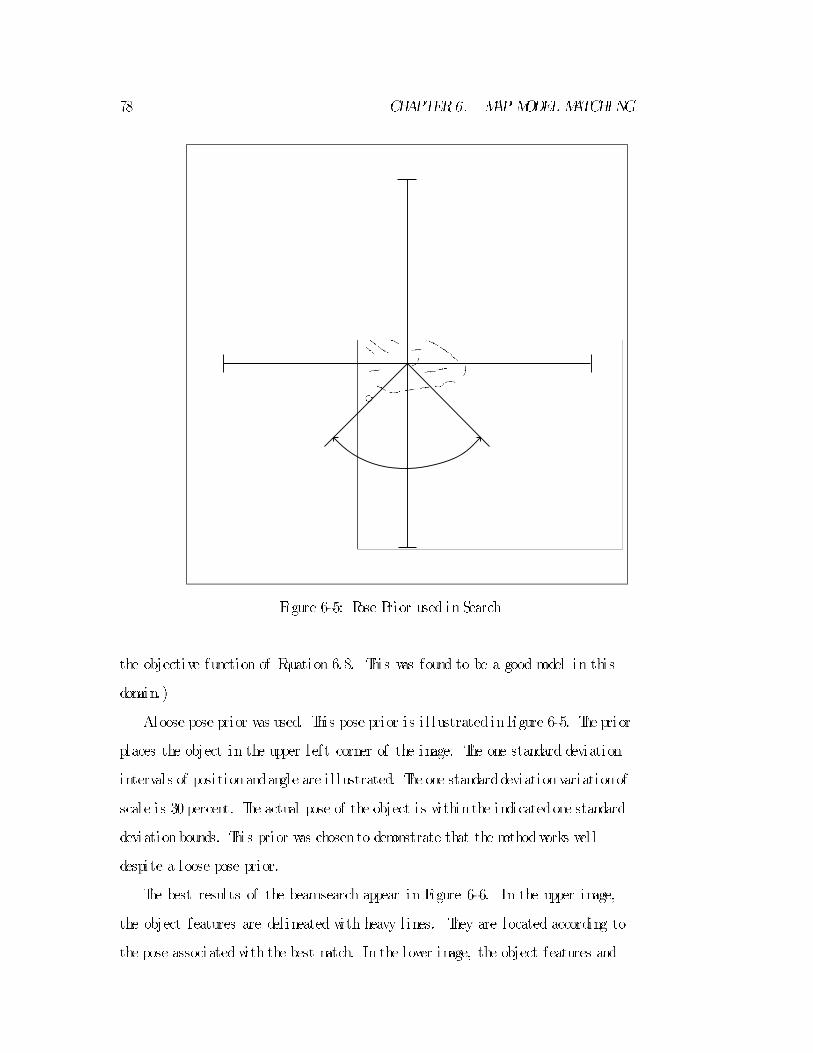
78 CHAPTER6. MAPMODEL MATCHING
Figure 6-5: Pose Prior used in Search
the objective function of Equation 6.8. This was found to be a good model in this
domain.)
Aloose pose prior was used. This pose prior i s i l lustrated inFigure 6-5. The prior
places the object in the upper left corner of the image. The one standard deviation
intervals of positionandangle are i l lustrated. The one standarddeviationvariationof
scale i s 30 percent. The actual pose of the object i s withinthe indicatedone standard
deviationbounds. This prior was chosento demonstrate that the methodworks wel l
despite a loose pose prior.
The best results of the beamsearch appear in Figure 6-6. In the upper image,
the object features are del ineated with heavy l ines. They are located according to
the pose associatedwith the best match. In the lower image, the object features and

6. 3. SEARCHI NPOSE SPACE 79
image features are i l lustrated, whi le the 18 correspondences associatedwith the best
matchappear as heavy l ines anddots.
The object features located according to the poses associated with the �ve best
matches are seen in Figure 6-7. The results are di�cult to distinguish because the
poses are very simi lar.
6.3 Search inPose Space
This sectionwi l l explore searching the MMMobjective function in pose space. Con-
nections to robust chamfer matching wi l l be described.
Apose estimate is sought byorderingthe searchfor maximaof theMMMobjective
function as fol lows,
�=argmax�
max�
L(�; �) :
Substituting the objective function fromEquation 6.6 yields
�=argmax�
max�
Xi j : �i=M j
[�i j�1
2(Yi �P(M j; �))
T �1i j(Yi �P(M j ; �))] :
The pose prior termhas been dropped in the interest of clari ty. It would be easi ly
retained as an additional quadratic term.
This equationmay be simpl i�edwith the fol lowing de�nition,
Di j(x) �1
2x
T
�1i jx :
Di j(x) may be thought of as a general ized squared distance between observed and
predicted features. It has been cal led the squaredMahalonobis distance [22] .
The pose estimator may nowbe written as
�=argmax�
max�
Xi j : �i=M j
[�i j�D i j(Yi �P(M j; �))] ;
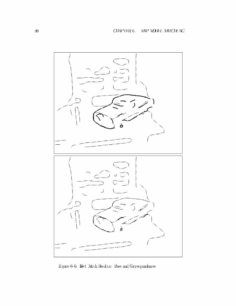
80 CHAPTER6. MAPMODEL MATCHING
Figure 6-6: Best MatchResults: Pose andCorrespondences

6. 3. SEARCHI NPOSE SPACE 81
Figure 6-7: Best Five MatchResults
or equivalently, as a minimization rather that maximization,
�=argmin�
min�
Xi j : �i=M j
[Di j(Yi �P(M j; �))�� i j] :
The sumis taken over those image features that are assigned to model features
(not the background) in the match. It may be re-written in the fol lowing way,
�=argmin�
Xi
min�i
8><>: 0 i f �i =?
Di j(Yi �P(M j; �))�� i j i f �i =M j
;
or as
�=argmin�
Xi
min(0; minj
Di j(Yi �P(M j; �))�� i j) :
If the correspondence rewardis independent of the model feature (this holds when
oriented stationary statistics are used), � i j =� i. In this case, � i may be added to

82 CHAPTER6. MAPMODEL MATCHING
each termin the sumwithout a�ecting the minimizing pose, yielding the fol lowing
formfor the pose estimator,
�=argmin�
Xi
min(� i; minj
Di j(Yi �P(M j; �))) : (6:11)
This objective function is easi ly interpreted { it i s the sum, taken over image
features of a saturated penalty. The penalty (before saturation) is the smal lest gen-
eral ized squared distance fromthe observed image feature to some projected model
feature. The penalty min j Di j(x�P(M j; �)) has the formof a Voronoi surface, as
described by Huttenlocher et. al . [42] . They describe a measure of simi lari ty on
image patterns, the Hausdor� distance, that is the upper envelope (maximum) of
Voronoi surfaces. The measure usedhere di�ers inbeing saturated, andbyusing the
sumof Voronoi surfaces, rather than the upper envelope. In their work, the upper
envelope o�ers some reduction in the complexity of the measure, and faci l i tates the
use of methods of computational geometry for expl ici tly computing the measure in 2
and 3 dimensional spaces.
Computational geometry methods might be useful for computing the objective
function of Equation 6.11. In higher dimensional pose spaces (4 or 6, for example)
KD-tree methods may be the only such techniques currently avai lable. Breuel has
usedKD-tree searchalgorithms in feature matching.
Next aconnectionwi l l be shownbetweenMMMsearchinpose space andamethod
of robust chamfer matching. First, the domainof MMMis simpl i�ed in the fol lowing
way. Ful l stationarity of feature uctuations is assumed (as covered in Section 3.3).
Further, the feature covariance is assumed to be isotropic. With these assumptions
we have i j=�2I, andD i j=
12�2j xj2. Additional ly, assuming constant background
probabi l i ty, we have � i j =�. The pose estimator of Equation 6.11 may nowbe

6. 3. SEARCHI NPOSE SPACE 83
written in the fol lowing simpl i�ed form,
�=argmin�
Xi
min(�; minj
(1
2� 2j Yi �P(M j; �)j 2)) :
When the projection function is l inear, invertible, and distance preserving, (2D
and3Drigidtransformations satisfythese properties), the estimator maybe expressed
as fol lows,
�=argmin�
Xi
min(�; minj
(1
2� 2j P�1(Yi; �)�M jj2)) :
This may be further simpl i�ed to
�=argmin�
Xi
min(�; d 2(P�1(Yi; �))) ; (6:12)
by using the fol lowing de�nition of a minimumdistance function.
d(x) � 1p2�
minj
j x�M j j : (6:13)
Chamferingmethods maybe usedtotabulate approximations of d 2(x) inanimage-
l ike array that is indexed by pixel coordinates. Chamfer-based approaches to image
registration problems use the array to faci l i tate fast evaluation of pose objective
functions. Barrowet al . [3] describe an early method where the objective function
is the sumover model features of the distance fromthe projected model feature to
the nearest image feature. Borgefors [8] recommends the use of RMSdistance rather
than summed distance in the objective function.
Recently, Jiang et al . [47] described a method of robust chamfer matching. In
order to make the method less susceptible to disturbance by outl iers and occlusions,
they added saturation to the RMS objective function of Borgefors. Their objective

84 CHAPTER6. MAPMODEL MATCHING
function has the fol lowing form
1
3(1
n
Xj
min(t 2; d
2j))
1
2 ;
where d 2ji s the squared distance fromthe j' th projected model point to the near-
est image point. Aside fromthe constants and square root, which don't a�ect the
minimizing pose, this objective function is equivalent to Equation 6.12 i f the role of
image andmodel features is reversed, and the sense of the projection function is in-
verted. Jiang et al . showimpressive results using robust chamfer matching to register
multi -modal 3Dmedical imagery.
6.4 Extensions
MAPModel Matching performs wel l on low resolution imagery in which feature
uncertainty is signi�cant. It could be used to bootstrap a coarse-�ne approach to
model matching, yielding good results with reasonable running times. Coarse-�ne
approaches have proven successful in stereo matching appl ications. (See Grimson
[33] and Barnard [2] . ) Acoarse-�ne strategy is straightforward in the framework
described here. In a hierarchy, the pose estimate fromsolving the objective function
at one scale i s used as a prior for the estimation at the next. Having a goodprior on
the pose wi l l greatly reduce the amount of searching required at high resolution.
Finding a tractable model that incorporates pose dependent visibi l i ty conditions
wouldbe useful for applying MMMinnon view-based recognition.
6.5 RelatedWork
The HYPERvision systemof Ayache and Faugeras [1] uses sequential l inear-least-
squares pose estimation as wel l as the l inear 2Dpoint feature and projectionmodel
describedinSection5.2. HYPERis describedas a searchalgorithm. Di�erent cri teria

6. 5. RELATEDWORK 85
are used to evaluate candidate matches and to evaluate competing \whole" hypothe-
ses. An ad hoc threshold is used for testing a continuous measure of the metrical
consistency of candidate match extensions. Whole match hypotheses are evaluated
according to the amount of image feature accounted for { although not according to
overal l metrical consistency. HYPERworks wel l on real images of industrial parts.
Goad outl ined a Bayesian strategy of match evaluation based on feature and
backgroundstatistics inhis paper onautomatic programming for model -basedvision
[29] . In his system, searchwas control led by thresholds on probabi l i stic measures of
the rel iabi l i ty andplausibi l i ty of matches.
Lowe describes ingeneral terms the appl icationof Bayesiantechniques inhis book
on Visual Recognition [51] . He treats the minimization of expected running time of
recognition. In addition he discusses selection among numerous objects.
Object recognitionmatching systems oftenuse a strategythat canbe summarized
as a search for the maximal matching that is consistent. Consistency is frequently
de�nedtomeanthat thematchingimage feature is within�nite bounds of i ts expected
position(boundederror models). Cass' system[14] i s one example. Suchanapproach
may be cast in the framework de�ned here by assuming uni formprobabi l i ty density
functions for the feature deviations. Pose solution with this approach is l ikely to be
more compl icated than the sequential l inear-least-squares method that can be used
when feature deviations have normal models. Cass' approach e�ectively �nds the
global optimumof its objective function. It performs wel l onoccludedor fragmented
real images.
Beveridge, Weiss andRiseman[6] use anobjective function for l ine segment based
recognition that is simi lar to the one described here. In their work, the penalty for
deviations is quadratic, whi le the reward for correspondence is non-l inear (exponen-
tial ) in the amount of missing segment length. (By contrast, the rewarddescribed in
this paper is, for stationary models, l inear in the length of aggregate features. ) The
trade-o� parameters in their objective function were determined empirical ly. Their
86 CHAPTER6. MAPMODEL MATCHING
systemgives goodperformance in a domain of real images.
Burns andRiseman [12] andBurns [11] describe a classi�cationbasedrecognition
system. They focus onthe use of descriptionnetworks for e�ciently searching among
multiple objects with a recursive indexing scheme.
HansonandFua [27] [26] describe a general objective functionapproach to image
understanding. They use a minimumdescription length (MDL) criterion that is
designedtoworkwithgeneric object models. The approachpresentedhere is tai lored
for speci�c object models.
6.6 Summary
AMAPmodel matching technique for visual object recognition has been described.
The resulting objective function has a simple formwhen normal feature deviation
models and l inear projection models are used. Experimental results were shown
indicating that MAPModel Matching works wel l in lowresolutionmatching, where
feature deviations are signi�cant. Relatedworkwas discussed.

Chapt er 7
Pos t er i or Margi nal Pos e
Es t i mat i on
Inthe previous chapter onMAPModel Matching the object recognitionproblemwas
posed as an optimization problemresulting froma statistical theory. In that formu-
lation, complete hypotheses consist of a description of the correspondences between
image and object features, as wel l as the pose of the object. The methodwas shown
to provide e�ective evaluations of matchandpose.
The formulationof recognitionthat is describedinthis chapter, Posterior Marginal
Pose Estimation 1 (PMPE), bui lds onMAPModel Matching. It provides a smooth
objective function for evaluating the pose of the object { without commitment to a
particular match. The pose is the most important aspect of the problem, inthe sense
that knowing the pose enables grasping or other interactionwith the object.
In this chapter, the objective function is explored by probing in selected parts of
pose space. The domain of these experiments is features derivedfromsynthetic laser
radar range imagery, and grayscale video imagery. Al imited pose space search is
performed in the video experiment.
In Chapter 8 the Expectation { Maximization (EM) algorithmis discussed as a
1An early version of thi s work appeared in [76]
87
88 CHAPTER7. POSTERIORMARGINAL POSE ESTIMATION
means of searching for local maxima of the objective function in pose space.
Additional experiments in object recognition using the PMPEobjective function
are described in Chapter 10. There, the EMalgorithmis used in conjunction with
an indexing method that generates initial hypotheses.
7.1 Objective Function for Pose
The fol lowingmethodwas motivatedbythe observationthat inheuristic searches over
correspondences with the objective function of MAPModel Matching, hypotheses
having implausible matches scored poorly in the objective function. The impl ication
was that summingposterior probabi l i tyover al l thematches (at a speci�c pose) might
provide a goodpose evaluator. This has proven to be the case. Although intuitively,
this might seeml ike an oddway to evaluate a pose, i t i s at least democratic in that
al l poses are evaluated in the same way. The resulting pose estimator is smooth,
and is amenable to local search in pose space. It i s not tied to speci�c matches {
it i s perhaps in keeping withMarr's recommendation that computational theories of
vision should try to satisfy a principle of least commitment [52] .
Additional motivation was provided by the work by Yui l le, Geiger and B�ultho�
on stereo [78] . They discussed computing disparities in a statistical theory of stereo
where a marginal i s computed over matches.
InMAPModel Matching, joint hypotheses of match andpose were evaluatedby
their posterior probabi l i ty, given an image { p(�; � j Y). � and � stand for cor-
respondences and pose, respectively, and Y for the image features. The posterior
probabi l i ty was bui l t fromspeci�c models of features and correspondences, objects,
and projection that were described in the previous chapters. The present formula-
tion wi l l �rst be described using the independent correspondence model . Use of the
Markov correspondence model wi l l be described in the fol lowing section.
Here we use the same strategy for evaluating object poses: they are evaluated

7. 1. OBJECTI VE FUNCTIONFORPOSE 89
by their posterior probabi l i ty, given an image: p(� j Y). The posterior probabi l i ty
densityof the pose maybe computedfromthe joint posterior probabi l i tyonpose and
match, by formal ly taking the marginal over possible matches:
p(�j Y) =X�
p(�; �j Y) :
In Section 6.1, Equation 6.4, p(�; �j Y) was obtained via Bayes' rule fromprob-
abi l i stic models of image features, correspondences, and the pose. Substi tuting for
p(�; �j Y), the posterior marginal may be written as
p(�j Y) =X�
p(Y j �; �)p(�; �)p(Y)
: (7:1)
Using equations 2.1 (the independent feature model) and6.2, we mayexpress the
posterior marginal of � in terms of the component densities:
p(�j Y) = 1
p(Y)
X�1
X�2
� � �X�n
Yi
p(Y i j �; �)Yi
p(� i)p(�)
or
p(�j Y) = p(�)
p(Y)
X�1
X�2
� � �X�n
Yi
[p(Y i j �i; �)p(� i)] :
Breaking one factor out of the product gives
p(�j Y) = p(�)
p(Y)
X�1
X�2
� � �X�n
"n�1Yi =1
[ p(Y i j �i; �)p(� i)]
#p(Y n j �n; �)p(� n) ;
or
p(�j Y) = p(�)
p(Y)
X�1
X�2
� � �X�n�1
"n�1Yi =1
[ p(Y i j �i; �)p(� i)]
# 24X�n
p(Y n j �n; �)p(� n)
35:
90 CHAPTER7. POSTERIORMARGINAL POSE ESTIMATION
Continuing in simi lar fashion yields
p(�j Y) = p(�)
p(Y)
Yi
24X�i
p(Y i j �i; �)p(� i)
35:
This may be written as
p(�j Y) = p(�)
p(Y)
Yi
p(Y i j �) ; (7:2)
since
p(Y i j �) =X�i
p(Y i j �i; �)p(� i) : (7:3)
Spl i tting the � i suminto its cases gives,
p(Y i j �) =p(Y i j �i =?; �)p(� i =?) +XMj
p(Y i j �i =M j; �)p(� i =M j) :
Substituting the densities assumed in the model of Section 6.1 in Equations 6.1 and
2.2 then yields
p(Y i j �) =1
W1 � � � WvBi +
XMj
G ij(Yi �P(M j ; �))
1�B i
m
: (7:4)
Instal l ing this into Equation 7.2 leads to
p(�j Y) = B1B2 � � � Bn(W1W2 � � � Wv)n
p(�)
p(Y)
Yi
241+ XMj
W1 � � � Wvm
1�B i
Bi
G ij(Yi �P(M j; �))
35.
As inSection6.1 the objective function for Posterior Marginal Pose Estimation is
de�ned as the scaled logarithmof the posterior marginal probabi l i ty of the pose,
L(�) �ln"p(�j Y)
C
#;

7. 2. USI NGTHEMARKOVCORRESPONDENCEMODEL 91
where, as before,
C=B1B2 � � � Bn
(W1W2 � � � Wv)n(2�)
�z2 j �j
�1
2
1
p(Y):
This leads to the fol lowing expression for the objective function(use of a normal pose
prior i s assumed)
L(�) =� 1
2(��� o)
T
�1�(��� 0)+
Xi
ln
241+ XMj
W1 � � � Wvm
1�B i
Bi
G ij(Yi �P(M j; �))
35(7:5)
.
This objective function for evaluating pose hypotheses is a smoothfunctionof the
pose. Methods of continuous optimization may be used to search for local maxima,
although starting values are an issue.
The �rst termin the PMPEobjective function (Equation 7.5) is due to the pose
prior. It i s a quadratic penalty for deviations fromthe nominal pose. The second
termessential lymeasures the degree of al ignment of the object model withthe image.
It i s a sumtakenover image features of a smooth non-l inear function that peaks up
positivelywhenthe pose brings object features intoal ignment withthe image feature
in question. The logarithmic termwil l be near zero i f there are no model features
close to the image feature in question.
In a straightforward implementation of the objective function, the cost of evalu-
ating a pose is O(mn), since it i s essential ly a non-l inear double sumover image and
model features.
7.2 Using the MarkovCorrespondence Model
When the Markov Correspondence model of Section 2.3 is used instead of the in-
dependent correspondence model , the summing techniques of the previous section
no longer apply. Because of this, a computational ly attractive closed formformula
92 CHAPTER7. POSTERIORMARGINAL POSE ESTIMATION
for the posterior probabi l i ty no longer obtains. Nevertheless, i t wi l l be shown that
the posterior probabi l i ty at a pose can sti l l be e�ciently evaluated using dynamic
programming.
Referring to Equation 7.1, and using the independence of match and pose in the
prior (discussed in Section 6.1), the posterior marginal probabi l i ty of a pose may be
written as fol lows,
p(�j Y) =X�
p(Y j �; �)p(�)p(�)p(Y)
:
Using Equations 2.3 and 6.1,
p(�j Y) = p(�)
p(Y)
X�
p(Y 1 j �1; �)p(Y 2 j �2; �) � � � p(Yn j �n; �) q(� 1)q(� 2) � � � q(�n)
r1(�1;�2)r2(�2;�3) � � � rn�1(�n�1;�n)
This may be re-written as fol lows,
p(�j Y) = p(�)
p(Y)
X�1�2:: : �n
"nYi =1
ci(�i)n�1Yi =1
ri(�i;�i +1)
#; (7:6)
where
ci �p(Y i j �i; �)q(� i) :
Here, the dependence of c on�has been suppressed for notational brevity.
Next it wi l l be shownthat p(�j Y) may be written using a recurrence relation:
p(�j Y) = p(�)
p(Y)
X�n
hn�1(�n)cn(�n) ; (7:7)
where
h1(a) �Xb
c1(b)r 1(b; a) (7:8)
and
hn+1 (a) �Xb
hn(b)c n+1 (b)r n+1 (b; a) : (7:9)

7. 2. USI NGTHEMARKOVCORRESPONDENCEMODEL 93
Expanding Equation 7.7 in terms of the recurrence relation,
p(�j Y) = p(�)
p(Y)
X�n
24X�n�1
hn�2(�n�1)cn�1(�n�1)rn�1(�n�1;�n)
35cn(�n) ;
or
p(�j Y) = p(�)
p(Y)
X�n�1 �n
hn�2(�n�1)nY
i =n�1
ci(�i) rn�1(�n�1;�n) :
Again using the recurrence relation,
p(�j Y) = p(�)
p(Y)
X�n�1 �n
24X�n�2
hn�3(�n�2)cn�2(�n�2)rn�2(�n�2;�n�1)
35
�nY
i =n�1
ci(�i) rn�1(�n�1;�n) ;
or
p(�j Y) = p(�)
p(Y)
X�n�2 �n�1 �n
hn�3(�n�2)nY
i =n�2
ci(�i)n�1Yi =n�2
ri(�i;�i +1) :
Continuing in simi lar fashion leads to
p(�j Y) = p(�)
p(Y)
X�2�3: : : �n
h1(�2)nYi =2
ci(�i)n�1Yi =2
ri(�i;�i +1) ;
andnowusing the base expression for h 1(� ),
p(�j Y) = p(�)
p(Y)
X�2�3: : : �n
24X�1
c1(�1)r1(�1;�2)
35 nYi =2
ci(�i)n�1Yi =2
ri(�i;�i +1) ;
or �nal ly,
p(�j Y) = p(�)
p(Y)
X�1�2: : : �n
"nYi =1
ci(�i)n�1Yi =1
ri(�i;�i +1)
#;
which is the same as Equation 7.6. This completes the veri�cation of Equation 7.7.
Next, a dynamic programming algorithmwil l be described that e�ciently evalu-
ates an objective function that is proportional to the posterior marginal probabi l i ty
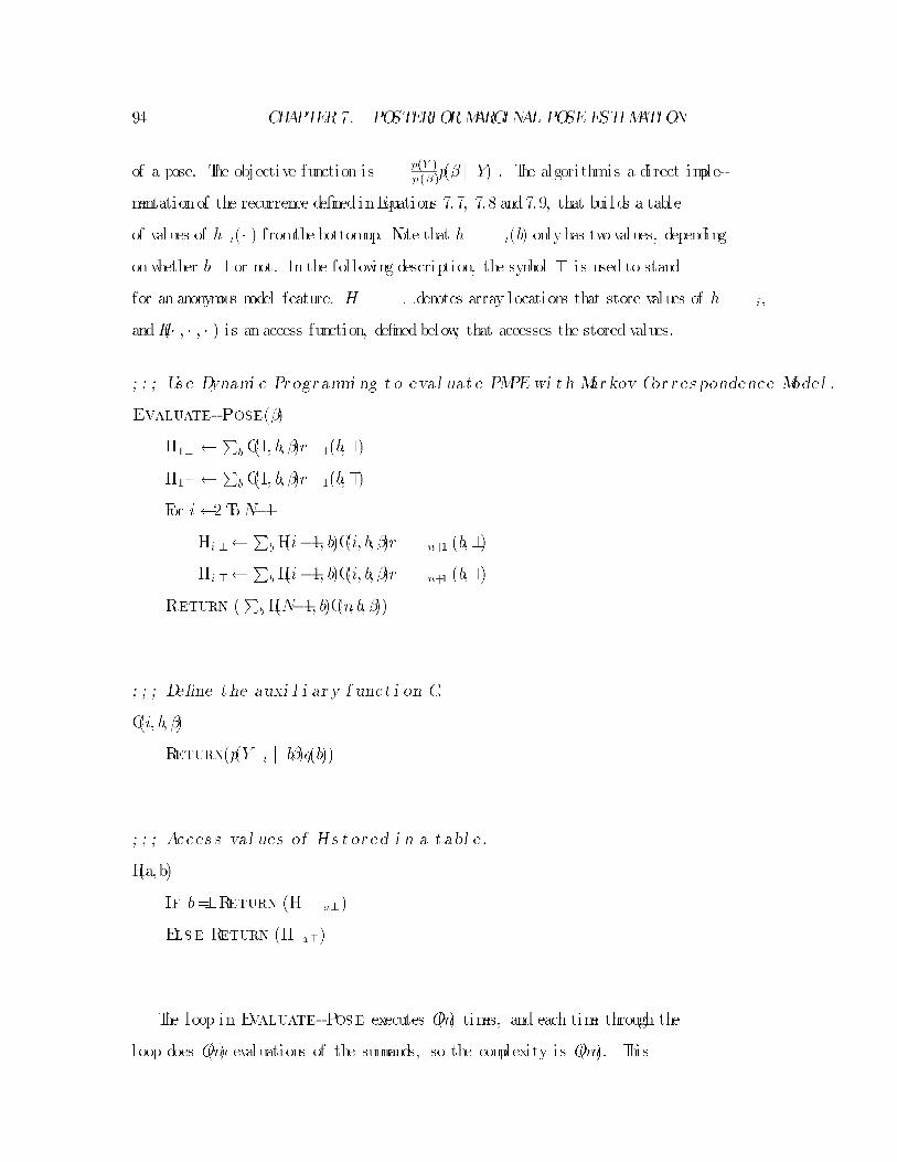
94 CHAPTER7. POSTERIORMARGINAL POSE ESTIMATION
of a pose. The objective function isp(Y )
p(�)p(� j Y) . The algorithmis a direct imple-
mentationof the recurrence de�ned inEquations 7.7, 7.8 and7.9, that bui lds a table
of values of h i(� ) fromthe bottomup. Note that h i(b) onlyhas twovalues, depending
onwhether b=?or not. In the fol lowing description, the symbol > i s used to stand
for an anonymous model feature. H � �denotes array locations that store values of h i,
andH(� ; � ; � ) i s an access function, de�nedbelow, that accesses the stored values.
; ; ; Us e Dynami c Pr ogr ammi ng t o eval uat e PMPEwi t h Mar kov Cor r es pondence Model .
Evaluate-Pose(�)
H1? PbC(1; b; �)r 1(b;?)
H1> PbC(1; b; �)r 1(b;>)
For i 2 ToN�1
Hi ? PbH(i�1; b)C(i; b; �)r n+1 (b;?)
Hi > PbH(i�1; b)C(i; b; �)r n+1 (b;>)
Return (PbH(N�1; b)C(n; b; �))
; ; ; De�ne t he auxi l i ar y f unct i on C.
C(i; b; �)
Return(p(Y i j b�)q(b))
; ; ; Acces s val ues of H s t or ed i n a t abl e .
H(a,b)
If b=?Return (H a?)
Else Return (H a>)
The loop in Evaluate-Pose executes O(n) times, and each time through the
loop does O(m) evaluations of the summands, so the complexity is O(mn). This
7. 3. RANGE IMAGEEXPERIMENT 95
has the same complexityas a straightforwardimplementationof the PMPEobjective
functionwhen the Markovmodel i s not used (Equation 7.5).
The summing technique used here was described by Cheeseman [17] in a paper
about using maximum-entropymethods in expert systems.
7.3 Range Image Experiment
Anexperiment investigating the uti l i ty of Posterior Marginal Pose Estimation is de-
scribed in this section. Additional experiments are described inChapter 10.
The objective functionof Equation7.5was sampledinadomainof synthetic range
imagery. The feasibi l i ty of coarse-�ne searchmethods was investigated by sampl ing
smoothed variants of the objective function.
7.3.1 Preparationof Features
The preparation of the features used in the experiment is summarized inFigure 7-1.
The features were oriented-range features, as described in Section 5.4. Two sets of
features were prepared, the \model features", and the \image features".
The object model features were derived froma synthetic range image of anM35
truck that was created using the ray tracing programassociatedwith the BRLCAD
Package [23] . The raytracer was modi�edto produce range images insteadof shaded
images. The synthetic range image appears in the upper left of Figure 7-2.
In order to simulate a laser radar, the synthetic range image describedabove was
corrupted with simulated laser radar sensor noise, using a sensor noise model that
is described by Shapiro, Reinhold, and Park [62] . In this noise model , measured
ranges are either val id or anomalous. Val idmeasurements are normal ly distributed,
and anomalous measurements are uni formly distributed. The corrupted range image
appears inFigure 7-2 on the right. To simulate post sensor processing, the corrupted
image was \restored" via a statistical restoration method of Menon andWel ls [56] .

96 CHAPTER7. POSTERIORMARGINAL POSE ESTIMATION
CAD MODEL
RAY TRACER
EXTRACTFEATURES
MODELFEATURES
ADDSENSORNOISE
RESTOREIMAGE
EXTRACT FEATURES
IMAGE FEATURES
TRANSFORMBY TEST POSE
DELETEHALF OFFEATURES
ADD EXTRAFEATURES
NOISYFEATURES
SYNTHETICRANGEIMAGE
NOISYRANGEIMAGE
RESTOREDRANGEIMAGE
Figure 7-1: Preparation of Features

7. 3. RANGE IMAGEEXPERIMENT 97
Figure 7-2: Synthetic Range Image, Noisy Range Image, andRestoredRange Image
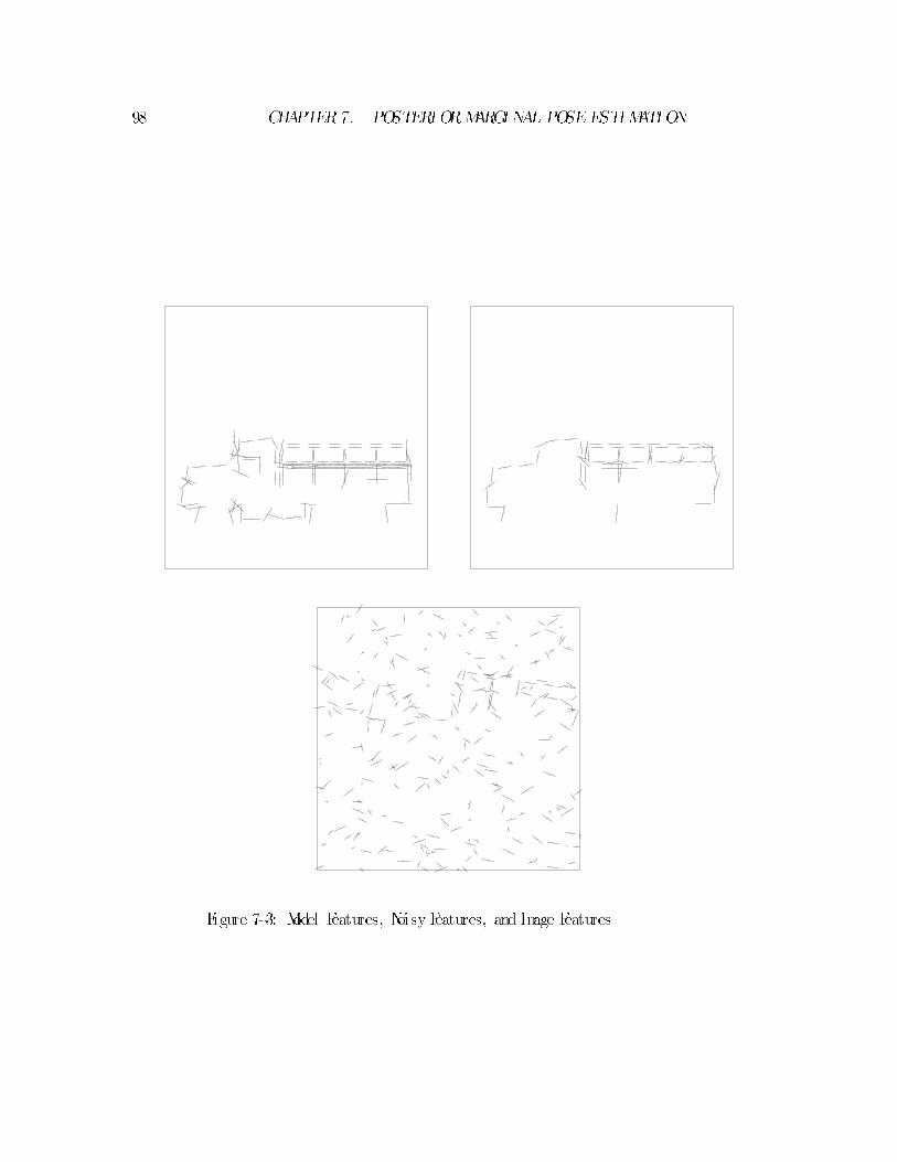
98 CHAPTER7. POSTERIORMARGINAL POSE ESTIMATION
Figure 7-3: Model Features, Noisy Features, and Image Features

7. 3. RANGE IMAGEEXPERIMENT 99
The restored range image appears in the lower position of Figure 7-2.
Orientedrange features, as described inSection5.4, were extracted fromthe syn-
thetic range image, for use as model features { and fromthe restored range image,
these are cal ledthe noisyfeatures. The features were extractedfromthe range images
in the fol lowing manner. Range discontinuities were located by thresholding neigh-
boring pixels, yielding range discontinuity curves. These curves were then segmented
into approximately 20-pixel -long segments via a process of l ine segment approxima-
tion. The l ine segments (eachrepresenting a fragment of a range discontinuitycurve)
were thenconvertedinto orientedrange features inthe fol lowingmanner. TheX and
Y coordinates of the feature were obtained fromthe mean of the pixel coordinates.
The normal vector to the pixels was gotten via least-squares l ine �tting. The range
to the feature was estimated by taking the mean of the pixel ranges on the near side
of the discontinuity. This information was packaged into an oriented-range feature,
as described in Section 5.4. The model features are shown in the �rst image of Fig-
ure 7-3. Each l ine segment represents one oriented-range feature, the ticks on the
segments indicate the near side of the range discontinuity. There are 113 suchobject
features.
The noisy features, derived fromthe restored range image, appear in the second
image of Figure 7-3. There are 62 noisy features. Some features have been lost due
to the corruption and restoration of the range image. The set of image features was
preparedfromthe noisy features byrandomlydeleting hal f of the features, transform-
ing the survivors according to a test pose, and adding su�cient randomly generated
features so that 18of the features are due to the object. The 248 image features appear
in the third image of Figure 7-3.
7.3.2 SamplingTheObjectiveFunction
The objective function of Equation7.5 was sampledalong four straight l ines passing
through the (known) location in pose space of the test pose. Oriented stationary

100 CHAPTER7. POSTERIORMARGINAL POSE ESTIMATION
statistics were used, as described in Section 3.3. The stationary feature covariance
was estimatedfroma handmatchdone withamouse betweenthe model features and
the noisy features. The background rate parameter Bwas set to 78.
Samples taken along a l ine through the location of the true pose in pose space,
paral lel to theXaxis are showninFigure 7-4. This corresponds tomoving the object
along the Xaxis. The �rst graph shows samples takenalong a 100 pixel length (the
image is 256 pixels square). The second graph of Figure 7-4 shows samples taken
along a 10 pixel length, and the third graph shows samples taken along a 1 pixel
length. The Xcoordinate of the test pose is 55.5, the third graph shows the peak of
the objective function to be in error by about one twentiethpixel .
Samples takenalong a l ine paral lel to the �axis of pose space are showninFigure
7-5. This corresponds to a simultaneous change in scale and angular orientation of
the object.
Eachof the above graphs represents 50 equal ly spaced samples. The samples are
joinedwith straight l ine segments for clari ty. Sampl ing was also done paral lel to the
Y and � axes with simi lar results.
The sampl ing described inthis sectionshows that inthe experimental domainthe
objective functionhas a prominent, sharppeak near the correct location. Some local
maxima are also apparent. The observed peak may not be the dominant peak { no
global searching was performed.
Coarse-Fine Sampl ing
Additional sampl ing of the objective of Equation7.5 was performedto investigate the
feasibi l i ty of coarse-�ne search techniques. Acoarse-�ne search method for �nding
maxima of the pose-space objective function would proceed as fol lows. Peaks are
initial ly located at a coarse scale. At each stage, the peak fromthe previous scale i s
used as the starting value for a searchat the next (less smooth) scale.
The objective function was smoothed by replacing the stationary feature covari -

7. 3. RANGE IMAGEEXPERIMENT 101
X Probes of Objective Function
0.0 10.0 20.0 30.0 40.0 50.0 60.0 70.0 80.0 90.0 100.0 110.0 0.0
5.0
10.0
15.0
20.0
25.0
30.0
35.0
40.0
45.0X Probes of Objective Function
50.0 51.0 52.0 53.0 54.0 55.0 56.0 57.0 58.0 59.0 60.0 61.0 0.0
5.0
10.0
15.0
20.0
25.0
30.0
35.0
40.0
45.0
X Probes of Objective Function
55.0 55.1 55.2 55.3 55.4 55.5 55.6 55.7 55.8 55.9 24.0
26.0
28.0
30.0
32.0
34.0
36.0
38.0
40.0
42.0
44.0
Figure 7-4: Objective Function Samples Along X-OrientedLine ThroughTest Pose,
Lengths: 100 Pixels, 10 Pixels, 1 Pixel
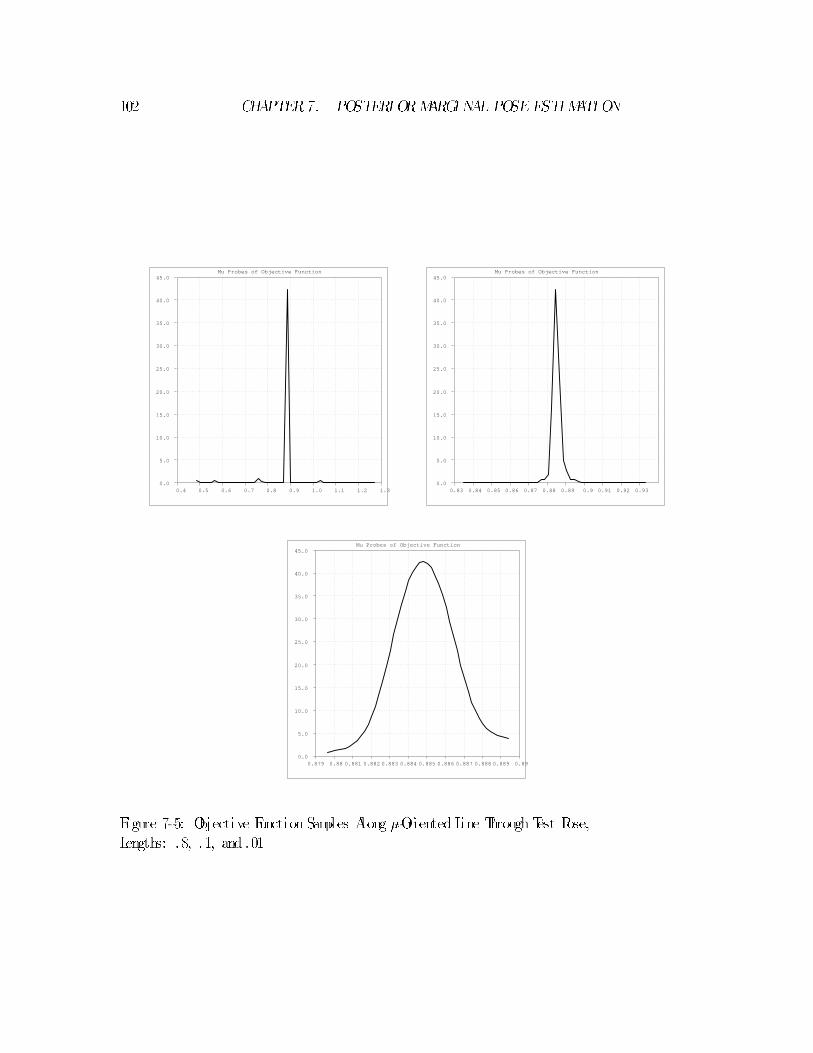
102 CHAPTER7. POSTERIORMARGINAL POSE ESTIMATION
Mu Probes of Objective Function
0.4 0.5 0.6 0.7 0.8 0.9 1.0 1.1 1.2 1.3 0.0
5.0
10.0
15.0
20.0
25.0
30.0
35.0
40.0
45.0Mu Probes of Objective Function
0.83 0.84 0.85 0.86 0.87 0.88 0.89 0.9 0.91 0.92 0.93 0.0
5.0
10.0
15.0
20.0
25.0
30.0
35.0
40.0
45.0
Mu Probes of Objective Function
0.879 0.88 0.881 0.882 0.883 0.884 0.885 0.886 0.887 0.888 0.889 0.89 0.0
5.0
10.0
15.0
20.0
25.0
30.0
35.0
40.0
45.0
Figure 7-5: Objective Function Samples Along �-OrientedLine ThroughTest Pose,
Lengths: .8, .1, and .01
7. 3. RANGE IMAGEEXPERIMENT 103
ance matrix in the fol lowingmanner:
+ s :
The e�ect of the smoothing matrix s i s to increase the spatial scale of the co-
variance matrices that appear in the objective function.
Probes along theXaxis throughthe knownlocationof the test pose, withvarious
amounts of smoothing are shown in Figure 7-6. The smoothing matrices used in the
probing were as fol lows, in the same order as the �gures.
DIAG((:1) 2; (:1)2; (10:0) 2
; (10:0) 2) ;
DIAG((:025) 2; (:025) 2
; (2:5) 2; (2:5) 2) ;
and
DIAG((:01) 2; (:01) 2
; 1:0; 1:0) :
where DIAG(� ) constructs diagonal matrices fromits arguments. These smoothing
matrices were determined empirical ly. (No smoothing was performed in the fourth
�gure.)
These smoothed sampl ing experiments indicate that coarse-�ne search may be
feasible in this domain. In Figure 7-6 it i s apparent that the peak at one scale may
be used as a starting value for local search in the next scale. This indicates that a
�nal l ine searchalong theXaxis coulduse the coarse �ne strategy. It i s not su�cient
evidence that such a strategy wi l l work in general . As before, there is no guarantee
that the locatedmaximumis the global maximum.

104 CHAPTER7. POSTERIORMARGINAL POSE ESTIMATION
X Probes of Objective Function
-60.0 -40.0 -20.0 0.0 20.0 40.0 60.0 80.0 100.0 120.0 140.0 160.0 0.0
20.0
40.0
60.0
80.0
100.0
120.0X Probes of Objective Function
0.0 10.0 20.0 30.0 40.0 50.0 60.0 70.0 80.0 90.0 100.0 110.0 0.0
10.0
20.0
30.0
40.0
50.0
60.0
X Probes of Objective Function
0.0 10.0 20.0 30.0 40.0 50.0 60.0 70.0 80.0 90.0 100.0 110.0 0.0
10.0
20.0
30.0
40.0
50.0
60.0X Probes of Objective Function
0.0 10.0 20.0 30.0 40.0 50.0 60.0 70.0 80.0 90.0 100.0 110.0 0.0
5.0
10.0
15.0
20.0
25.0
30.0
35.0
40.0
45.0
Figure 7-6: XProbes in SmoothedObjective Function

7. 4. VI DEOIMAGEEXPERIMENT 105
7.4 Video Image Experiment
In this section, another experiment with the PMPEobjective function is described.
The features are point-radius features derived fromvideo images. Alocal search in
pose space is carried out, and the objective function, and a smoothed variant, are
probed in the vicinity of the peak.
7.4.1 Preparationof Features
The features used in this experiment are the same as those used in the MAPModel
Matching correspondence searchexperiment reported inSection6.2. They are point-
radius features, as described in Section 5.3. The features appear inFigure 6-4.
7.4.2 SearchinPoseSpace
Asearchwas carried out in pose space froma starting value that was determinedby
hand. The search was implemented with Powel l ' s method [59] of multidimensional
non-l inear optimization. Powel l ' s methodis simi lar to the conjugate-gradient method,
but derivatives are not used. The l ine minimizations were carried out with Brent's
method [59] , which uses successive parabol ic approximations. The pose resulting
fromthe search is i l lustrated in Figure 7-7. This result i s close to the best result
fromthe MAPModel Matching correspondence search experiment. That result i s
reproduced here inFigure 7-8. It i s comforting that these two substantial ly di�erent
searchmethods (combinatorial versus continuous) provide simi lar answers in, at least,
one experiment.
7.4.3 SamplingTheObjectiveFunction
Samples were taken along four straight l ines passing through the peak in the objec-
tive function resulting fromthe search in pose space reported above. (In the range
experiment, sampl ing was done through the known true pose.) The results are i l lus-

106 CHAPTER7. POSTERIORMARGINAL POSE ESTIMATION
Figure 7-7: Results of Search inPose Space
Figure 7-8: Best Results fromMAPModel Matching Correspondence Search

7. 4. VI DEOIMAGEEXPERIMENT 107
X Probes of Objective Function
-50.0 -40.0 -30.0 -20.0 -10.0 0.0 10.0 20.0 30.0 40.0 50.0 60.0X
0.0
5.0
10.0
15.0
20.0
25.0
30.0
35.0
40.0
45.0
50.0
Objective Function
Y Probes of Objective Function
-60.0 -50.0 -40.0 -30.0 -20.0 -10.0 0.0 10.0 20.0 30.0 40.0 50.0Y
0.0
5.0
10.0
15.0
20.0
25.0
30.0
35.0
40.0
45.0
50.0
Objective Function
Mu Probes of Objective Function
0.9 0.92 0.94 0.96 0.98 1.0 1.02 1.04 1.06 1.08 1.1 1.12Mu
0.0
5.0
10.0
15.0
20.0
25.0
30.0
35.0
40.0
45.0
50.0
Objective Function
Nu Probes of Objective Function
-0.14 -0.12 -0.1 -0.08 -0.06 -0.04 -0.02 0.0 0.02 0.04 0.06 0.08Nu
0.0
5.0
10.0
15.0
20.0
25.0
30.0
35.0
40.0
45.0
50.0Objective Function
Figure 7-9: Probes of Objective FunctionPeak
trated in Figure 7-9. The peak in this data is not as sharp as the peak in the range
experiment reported in the previous section. This i s l ikely due to the fact that the
features used in the video experiment are substantial ly less constraining that those
used in the range experiment { whichhave good range information in them.
Sampl ing of the objective function with smoothing was also performed, as in
Section 7.3.2.

108 CHAPTER7. POSTERIORMARGINAL POSE ESTIMATION
Smoothing was performed at one scale. The smoothing matrix was
DIAG((:03) 2; (:03) 2
; (3:0) 2; (3:0) 2) :
Probing, performed in the same manner as in Figure 7-9 was performed on the
smoothed objective function. The results are shown in Figure 7-10. In comparison
to the range image experiment, local maxima are more of an issue here. This maybe
partly due to the backgroundfeatures here havingmore structure than the randomly
generated background features used in the range image experiment. Because of this,
anomalous pose estimates (where the pose corresponding to the global maximumof
the objective function is seriously in error) may be more l ikely in this domain than
in the range experiment.
7.5 Relation to Robust Estimation
This section describes a relationship between PMPE and robust estimation. By
simpl i fying the domain a robust estimator of position is obtained. Aconnection
between the simpl i�ed robust estimator andneural networks is discussed.
Consider the fol lowing simpl i�cations of the domain:
� drop the pose prior
� the object has one feature
� the image is one-dimensional withwidthW
� the pose is a scalar
� the projection function translates: P(� ; �) =�
.
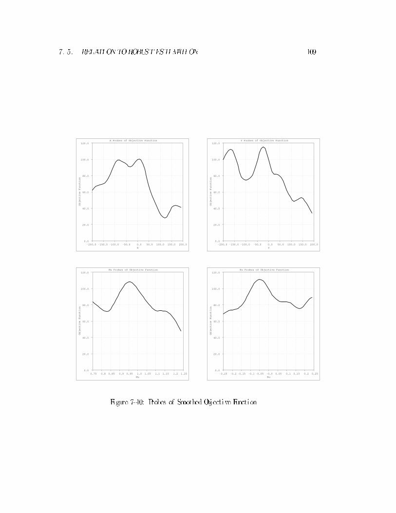
7. 5. RELATIONTOROBUSTESTIMATION 109
X Probes of Objective Function
-200.0 -150.0 -100.0 -50.0 0.0 50.0 100.0 150.0 200.0X
0.0
20.0
40.0
60.0
80.0
100.0
120.0
Objective Function
Y Probes of Objective Function
-200.0 -150.0 -100.0 -50.0 0.0 50.0 100.0 150.0 200.0Y
0.0
20.0
40.0
60.0
80.0
100.0
120.0
Objective Function
Mu Probes of Objective Function
0.75 0.8 0.85 0.9 0.95 1.0 1.05 1.1 1.15 1.2 1.25Mu
0.0
20.0
40.0
60.0
80.0
100.0
120.0
Objective Function
Nu Probes of Objective Function
-0.25 -0.2 -0.15 -0.1 -0.05 -0.0 0.05 0.1 0.15 0.2 0.25Nu
0.0
20.0
40.0
60.0
80.0
100.0
120.0
Objective Function
Figure 7-10: Probes of SmoothedObjective Function
110 CHAPTER7. POSTERIORMARGINAL POSE ESTIMATION
With these simpl i�cations, the observationmodel of Equation 6.1 becomes
p(Y i j �; �) =
8><>:1W
i f �i =?
G�(Yi ��) otherwise;
where
G�(x) =1p2��
exp
� x
2
2� 2
!:
In this simpl i�ed domain �may be interpreted as a col lection of variables that de-
scribe the val idity of their corresponding measurements in Y. Thus, � i 6 =?may be
interpretedas meaning that Y i i s val id, and� i =?as Y i being inval id. p(Y i) i s de�ned
to be zero outside of the range [ �W
2;W
2] .
The prior on correspondences of Equation 2.2 takes the fol lowing form
p(� i) =
8><>: B i f � i =?
1�B otherwise:
UsingBayes' rule andthe independence of � i and�al lows the fol lowingprobabi l i ty
of a sample and its val idity,
p(Y i;�i j �) =p(Y i j �i; �)p(� i) =
8><>:B
Wi f �i =?
(1�B)G �(Yi ��) otherwise: (7:10)
The probabi l i ty of a sample maynowbe expressed by taking a marginal over the
probabi l i ty inEquation 7.10, as fol lows,
p(Y i j �) =X�i
p(Y i;�i j �) =B
W
+(1�B)G �(Yi ��) :
De�ning an objective function as a log l ikel ihood of �
L(�) =ln
"Yi
p(Y i j �)#;
7. 5. RELATIONTOROBUSTESTIMATION 111
leads to the analog of the PMPEobjective function for this simpl i�ed domain,
L(�) =Xi
ln
�B
W
+(1�B)G �(Yi ��)�: (7:11)
This may also be written
L(�) =Xi
S(Y i ��) (7:12)
where
S(x) =ln�B
W
+(1�B)G �(x)�;
This is the MaximumLikel ihood objective function for estimating the mean of a
normal populationof variance � 2, that is contaminatedwitha uni formpopulationof
widthW, where the fraction of the mixture due to the uni formpopulation is B.
The function S(x) i s approximately quadratic when the residual i s smal l , and
approaches a constant whenthe residual i s large. WhenBgoes to zero, S(x) becomes
quadratic, and the estimator becomes least squares, for the case of a pure normal
population. When �S(x) i s viewed as a penalty function, i t i s seen to provide a
quadratic penalty for smal l residuals, as least squares does, but the penalty saturates
when residuals become large. Robust estimation is concerned with estimators that
are, l ike this one, less sensitive to outl iers that least squares. As with many robust
estimators, the resulting optimization problemis more di�cult than least squares,
since the objective function is non-convex. This estimator fal l s into the class of re-
descending M-estimators as discussed byHuber [41] .
PMPEis somewhat di�erent fromrobust estimation inthat the saturating aspect
of the objective function not only decreases the in uence of \outl iers" (by analogy,
the background features), i t also reduces the in uence of image features that don't
correspond to (are not close to) a givenobject feature.

112 CHAPTER7. POSTERIORMARGINAL POSE ESTIMATION
7.5.1 ConnectiontoNeural NetworkSigmoidFunction
There is an important connection between the estimator of Equation 7.12 and the
sigmoid function of neural networks,
�(x) =1
1+exp(�x) :
The sigmoid function is a smooth variant of a logical switching function that has
been used for model ing neurons. It has been used extensively by the neural network
community in the construction of networks that classi fy and exhibit some forms of
learning behavior. The NETtalk neural network of Sejnowski and Rosenberg [61] i s
a wel l knowexample.
It turns out that, under some conditions on the parameters, the sigmoid function
of x2 i s approximatelyequal toS(x), ignoring shi fting andscal ing. This near equal i ty
is i l lustrated inFigure 7-11.
The two functions that are plotted in the �gure are
f(x) =2:0[�(x 2)�:5] and g(x) =ln[ :25+:75exp(�x 2)]
ln[ :25]:
The upper graphshows f(x)andg(x) plottedtogether, whi le the lower graphshows
their di�erence. It can be seen that they agree to better than one percent.
Because of this near equal i ty, for a special case of the parameters, a network that
evaluates the MLestimator of Equation 7.12 for a contaminated normal population
wi l l have the formi l lustrated inFigure 7-12.
This network, with its arrangement of sigmoid and sumunits seems to �t the
de�nition of a neural network.
The robust estimator of Equation7.12, andits neural networkapproximation, are
(approximately) optimal for locating a Gaussian cluster in uni formnoise.
Asimi lar neural network real ization of the PMPEobjective functionwould l ike-
wise be near optimal for locating an object against a uni formbackground.

7. 5. RELATIONTOROBUSTESTIMATION 113
f(x) and g(x)
-4.0 -3.0 -2.0 -1.0 0.0 1.0 2.0 3.0 4.0X
0.0
0.1
0.2
0.3
0.4
0.5
0.6
0.7
0.8
0.9
1.0
f(x) - g(x)
-4.0 -3.0 -2.0 -1.0 0.0 1.0 2.0 3.0 4.0
-0.008
-0.006
-0.004
-0.002
0.0
0.002
0.004
0.006
0.008
Figure 7-11: f(x) and g(x), and f(x)�g(x)
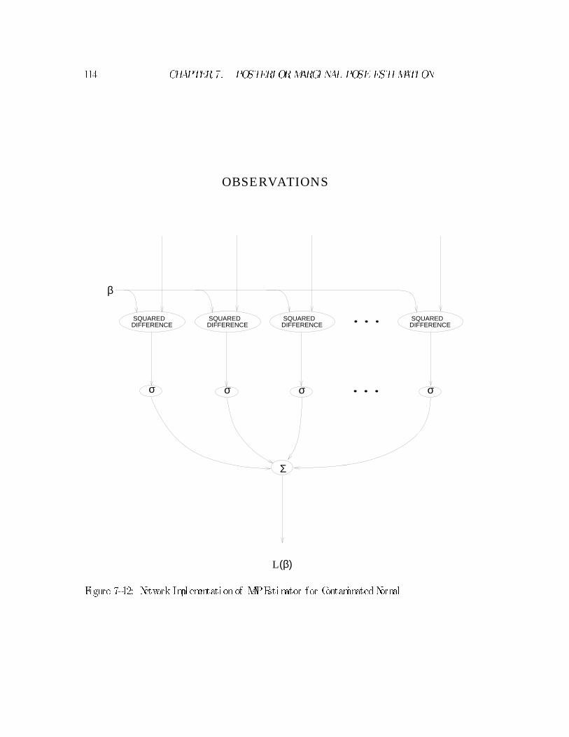
114 CHAPTER7. POSTERIORMARGINAL POSE ESTIMATION
SQUARED DIFFERENCE
SQUARED DIFFERENCE
SQUARED DIFFERENCE
SQUARED DIFFERENCE
σ σ σ σ
Σ
L(β)
β
OBSERVATIONS
Figure 7-12: Network Implementationof MAPEstimator for ContaminatedNormal

7. 6. PMPEEFFI CI ENCYBOUND 115
7.6 PMPEE�ciency Bound
This sectionprovides a lower boundonthe covariancematrixof the PMPEestimator.
Estimators of vector parameters (l ike pose) may be characterized by the covariance
matrix of the estimates they produce. The Cramer-Rao bound provides a lower
l imit for the covariance matrix of unbiased estimators. Unbiased estimators that
achieve this bound are cal l e�ci ent estimators. Discussions of estimator e�ciency
andCramer-Rao bounds appear in [63] and [72] .
The Cramer-Rao bound on the covariance matrix of estimators of � based on
observations of Xi s givenby the inverse of the Fisher informationmatrix,
COV( �) �I �1F(�) :
Here, COV(� ) denotes the covariance matrix of the randomvector argument. This
matrix inequal i tymeans that COV( �)�I �1F(�) i s positive semi-de�nite.
The Fisher informationmatrix is de�ned as fol lows,
IF (�) �E X([r� lnp(Xj �)] [r � lnp(Xj �)] T )
where r � i s the gradient with respect to �, whichyields a column-vector, andE X(� )
stands for the expected value of the argument with respect to p(X).
The covariance matrix, and the Cramer-Rao bound, of the PMPEestimator are
di�cult to calculate. Instead, the Cramer-Rao bound and e�ciency wi l l be deter-
mined for estimators that have access to both observed features Y i, and the corre-
spondences � i. The Cramer-Rao bound for these \complete-data" estimators wi l l be
found, and it wi l l be shownthat there are no e�cient complete-data estimators. Be-
cause of this, the PMPEestimator is subject to the same boundas the complete-data
estimators, and the PMPEestimator cannot be e�cient. This fol lows, because the
PMPEestimator can be considered to be technical ly a complete-data estimator that

116 CHAPTER7. POSTERIORMARGINAL POSE ESTIMATION
ignores the correspondence data.
In terms of the complete-data estimator, the Fisher informationhas the fol lowing
form,
IF (�) �E Y; �([r� lnp(Y;�j �)] [r � lnp(Y;�j �)] T ) : (7:13)
Assuming independence of feature coordinates and of correspondences, the prob-
abi l i ty of the complete-data is
p(Y;�j �) =Yi
p(Y i;�i j �) :
Using Bayes rule and the independence of �and�,
p(Y i;�i j �) =p(Y i j �i; �)p(� i) : (7:14)
Referring to Equations 6.1 and6.3, andusing constant backgroundprobabi l i tyB,
and l inear projection, the complete-data component probabi l i ty may be written as
fol lows,
p(Y i;�i j �) =
8><>:B
W1W2: : : Wvi f �i =?
1�Bm
G ij(Yi �M j�) i f � i =M j :
Workingtowards anexpressionfor the Fisher information, wedi�erentiate the complete-
data probabi l i ty to obtain
r� lnp(Y;�j �) =r � lnYi
p(Y i;�i j �) =Xi
r�p(Y i;�i j �)p(Y i;�i j �)
:
When� i =?, r �p(Y i;�i j �) =0, otherwise, in the case � i =M j,
r�p(Y i;�i j �) =r �
1�Bm
G ij(Yi �M j�) :

7. 6. PMPEEFFI CI ENCYBOUND 117
Di�erentiating the normal density (a formula for this appears in 8.3), gives
r�p(Y i;�i j �) =(�)1�Bm
G ij(Yi �M j�)M
T
j �1i j(Yi �M j�) ;
so that
r�p(Y i;�i j �)p(Y i;�i j �)
=�M T
j
�1i j(Yi �M j�) when � i =M j :
Then the gradient of the complete-data probabi l i tymay be expressed as
r� lnp(Y;�j �) =�X
i j : �i=M j
MT
j �1i j(Yi �M j�) :
Note that setting this expression to zero de�nes the MaximumLikel ihood estimator
for � in the complete-data case, as fol lows:
Xi j : �i=M j
MT
j �1i jYi =
Xi j : �i=M j
MT
j �1i jMj � ;
or
�=
0@ Xi j : �i=M j
M
T
j
�1i jMj
1A�1 Xi j : �i=M j
M
T
j
�1i jYi : (7:15)
This estimator is l inear in Y. The inverse has been assumed to exist { it wi l l exist,
providedcertainl inear independence conditions aremet, andenoughcorrespondences
tomodel features appear inthe match. This typical ly requires two to four correspon-
dences in the appl ications described here.
Returning to the Fisher information, we need to evaluate the expectation:
IF =E Y; �
0B@24 Xi j : �i=M j
M
T
j
�1i j�i j
35 24 Xi j : �i=M j
M
T
j
�1i j�i j
35T1CA ;

118 CHAPTER7. POSTERIORMARGINAL POSE ESTIMATION
where the ij' th residual has beenwritten as fol lows,
�i j�Y i �M j� :
Re-naming indices andpul l ing out the sums gives
IF =E Y; �
0@ Xi j : �i=M j
Xi0
j0: �i0=M j0
M
T
j
�1i j�i j�
T
i0j0
�1i0
j0Mj0
1A:
Referring to Equation 7.14, the expectationmay be spl i t andmovedas fol lows,
IF =E �
0@ Xi j : �i=M j
Xi0j0: �i0=M j0
M
T
j
�1i jEY j�(�i j�
T
i0j0) �1
i0j0Mj0
1A:
The inner expectation is over mutual ly independent Gaussian randomvectors, and
equals their covariance matrix when the indices agree, and is zero otherwise, so
IF =E �
0@ Xi j : �i=M j
Xi0j0: �i0=M j0
M
T
j
�1i j i j�i i0�j j0
�1i0j0Mj0
1A:
This expression simpl i�es to the fol lowing:
IF =E �
0@ Xi j : �i=M j
MT
j �1i jMj
1A:
The summaybe re-written in the fol lowingwaybyusing a delta function comparing
�i andM j,
IF =Xi j
E�
���iMj
�M
T
j �1i jMj =
Xi j
E�i
���iMj
�M
T
j �1i jMj :
The expectation is just the probabi l i ty that an image feature is matched to some
model feature. This i s 1�Bm
, so the Fisher informationmaybe written inthe fol lowing
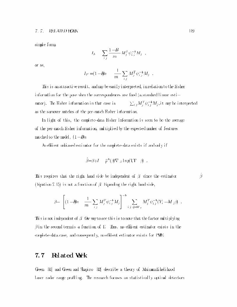
7. 7. RELATEDWORK 119
simple form,
IF =Xi j
1�Bm
MT
j �1i jMj ;
or as,
IF =(1�B)n 1
mn
Xi j
MT
j �1i jMj :
This is anattractive result, andmaybe easi ly interpreted, inrelationto the Fisher
information for the pose when the correspondences are �xed (a standard l inear esti -
mator). The Fisher information in that case isPi jM
T
j �1i jMj, i t may be interpreted
as the sumover matches of the per-matchFisher information.
In l ight of this, the complete-data Fisher information is seen to be the average
of the per-match Fisher information, multipl ied by the expected number of features
matched to the model , (1�B)n.
An e�cient unbiasedestimator for the complete-data exists i f and only i f
�=�+I �1F(�)r � lnp(Y;�j �) :
This requires that the right hand side be independent of �, since the estimator �
(Equation 7.15) is not a function of �. Expanding the right hand side,
�+
24(1�B)n 1
mn
Xi j
M
T
j
�1i jMj
35�1 Xi j : �i=M j
M
T
j
�1i j(Yi �M j�) :
This is not independent of �. One wayto see this i s tonote that the factor multiplying
� in the second termis a function of �. Thus, no e�cient estimator exists in the
complete-data case, and consequently, no e�cient estimator exists for PMPE.
7.7 RelatedWork
Green [31] and Green and Shapiro [32] describe a theory of MaximumLikel ihood
laser radar range pro�l ing. The research focuses on statistical ly optimal detectors
120 CHAPTER7. POSTERIORMARGINAL POSE ESTIMATION
and recognizers. The single pixel statistics are described by a mixture of uni form
and normal components. Range pro�l ing is implemented using the EMalgorithm.
Under some circumstances, least squares provides an adequate starting value. A
continuation-style variant is described, where a range accuracy parameter is varied
betweenEMconvergences froma coarse value to its true value. Green [31] computes
Cramer-Rao bounds for the complete-data case of MaximumLikel ihoodrange pro�le
estimator, and compares simulated and real -data performance to the l imits.
Cass [16] [15] describes an approach to visual object recognition that searches
in pose space for maximal al ignments under the bounded-error model . The pose-
space objective function used there is piecewise constant, and is thus not amenable
to continuous searchmethods. The search is based on geometric formulation of the
constraints on feasible transformations.
There are some connections betweenPMPEandstandardmethods of robust pose
estimation, l ike those described byHaral ick [38] , andKumar andHanson [48] . Both
can provide robust estimates of the pose of an object, based on an observed image.
The maindi�erence is that the standardmethods require speci�cationof the feature
correspondences, whi le PMPEdoes not { byconsidering al l possible correspondences.
PMPErequires a starting value for the pose (as do standardmethods of robust pose
estimation that use non-convex objective functions).
As mentioned above, Yui l le, Geiger and B�ultho� [78] discussed computing dis-
parities in a statistical theory of stereo where a marginal i s computed over matches.
Yui l le extends this technique [79] to other domains of vision and neural networks,
among themwinner-take-al l networks, stereo, long-range motion, the travel ing sales-
man problem, deformable template matching, learning, content addressable memo-
ries, andmodels of brain development. Inaddition to computing marginals over dis-
crete �elds, the Gibbs probabi l i ty distribution is used. This faci l i tates continuation-
style optimization methods by variation of the temperature parameter. There are
some simi lari ties betweenthis approachandusing coarse-�ne with the PMPEobjec-

7. 7. RELATEDWORK 121
tive function.
EdelmanandPoggio [24] describe a methodof 3Drecognition that uses a trained
General izedRadial Basis Function network. Their method requires correspondences
to be known during training and recognition. One simi lari ty between their scheme
andPMPEis that both are essential ly arrangements of smooth unimodal functions.
There is a simi lari ty between Posterior Marginal Pose Estimation and Hough
transform(HT) methods. Roughly speaking, HTmethods evaluate parameters by
accumulating votes in a discrete parameter space, based on observed features. (See
the survey paper by Il l ingworthandKittler [44] for a discussion of Houghmethods.)
In a recognition appl ication, as described here, the HTmethodwould evaluate a
discrete pose by counting the number of feature pairings that are exactly consistent
somewhere within the cel l of pose space. As stated, the HTmethod has di�culties
with noisy features. This i s usual ly addressed by counting feature pairings that are
exactly consistent somewhere nearby the cel l in pose space.
The uti l i ty of the HTas a stand-alone method for recognition in the presence of
noise is a topic of some controversy. This i s discussed by Grimson in [34] , pp. 220.
Perhaps this i s due to an unsuitable noise model impl ici t in the HoughTransform.
Posterior Marginal Pose Estimation evaluates a pose by accumulating the loga-
ri thmof posterior marginal probabi l i ty of the pose over image features.
The connectionbetweenHTmethods andparameter evaluationvia the logarithm
of posterior probabi l i tyhas beendescribedbyStephens [67] . Stephens proposes to cal l
the posterior probabi l i ty of parameters given image observations \The Probabi l i stic
Hough Transform". He provided an example of estimating l ine parameters from
image point features whose probabi l i ty densities were described as having uni form
and normal components. He also states that the method has been used to track 3D
objects, referring to his thesis [68] for de�nition of the methodused.

122 CHAPTER7. POSTERIORMARGINAL POSE ESTIMATION
7.8 Summary
Amethodof evaluating poses inobject recognition, Posterior Marginal Pose Estima-
tion, has been described. The resulting objective functionwas seen to have a simple
formwhen normal feature deviationmodels and l inear projectionmodels are used.
Limited experimental results were shownindicating that ina domainof synthetic
range discontinuityfeatures, the objective functionmayhave aprominent sharppeak
near the correct pose. Some local maxima were also apparent. Another experiment,
inwhichthe features were derived fromvideo images, was described. Connections to
robust estimationandneural networks were examined. Bounds onthe performance of
simpl i�edPMPEestimators were indicated, andrelationto other workwas discussed.
Chapt er 8
Expect at i on { Maxi mi zat i on
Al gor i t hm
The Expectation{ Maximization (EM) algorithmwas introduced in its general form
byDempster, RubinandLaird in1978 [21] . It i s oftenuseful for computing estimates
indomains having two sample spaces, where the events inone are unions over events
in the other. This si tuation holds among the sample spaces of Posterior Marginal
Pose Estimation(PMPE) andMAPModel Matching. Inthe original paper, the wide
general i ty of the EMalgorithmis discussed, along with several previous appearances
in special cases, and convergence results are described.
In this chapter, a speci�c formof the EMalgorithmis described for use with
PMPE. It i s used for hypothesis re�nement in the recognition experiments that are
described inChapter 10. Issues of convergence and implementationare discussed.
8.1 De�nition of EMIteration
In this section a variant of the EMalgorithmis presented for use with Posterior
Marginal Pose Estimation, whichwas describedinChapter 7. The fol lowingmodel ing
assumptions were used. Normal models are used for matched image features, whi le
123

124 CHAPTER8. EXPECTATION{ MAXIMI ZATIONALGORI THM
uni formmodels are usedfor unmatched(background) features. If aprior onthe pose is
avai lable, i t i s normal . The independent correspondence model i s used. Additional ly,
a l inear model i s used for feature projection.
In PMPE, the pose of an object, �, i s estimated by maximizing its posterior
probabi l i ty, given an image.
�=argmax�
p(�j Y) :
Anecessary condition for the maximumis that the gradient of the posterior prob-
abi l i ty with respect to the pose be zero, or equivalently, that the gradient of the
logarithmof the posterior probabi l i ty be zero:
0=r � lnp( �j Y) : (8:1)
InSection7.1, Equation7.2 the fol lowingformulawas givenfor the posterior prob-
abi l i tyof the pose of anobject, givenan image. This assumes use of the independent
correspondence model .
p(�j Y) = p(�)
p(Y)
Yi
p(Y i j �) :
Imposing the condition of Equation 8.1 yields the fol lowing,
0=r �
"ln
1
p(Y)+lnp( �) +
Xi
lnp(Y i j �)#
or
0=r�p( �)
p( �)+Xi
r�p(Y i j �)p(Y i j �)
: (8:2)
As in Equation 7.3, we may write the feature PDFconditioned on pose in the
fol lowing way,
p(Y i j �) =X�i
p(Y i j �i�)p(� i) ;
or, using the speci�c models assumedinSection7.1, as re ected inEquation7.4, and
8. 1. DEFI NI TI ONOF EMITERATION 125
using a l inear projectionmodel ,
p(Y i j �) =Bi
W1W2 � � � Wv+1�B i
m
Xj
G ij(Yi �M j�) :
The zero gradient condition of Equation 8.2 may nowbe expressed as fol lows,
0=r�p( �)
p( �)+Xi
1�Bi
m
Pjr�G ij
(Yi �M j�)Bi
W1W2� � � Wv+ 1�Bi
m
Pj G ij
(Yi �M j�):
With a normal pose prior,
p(�) =G �(��� 0) ; and r �p(�) =�p(�) �1
�(��� 0) :
The gradient of the other normal density is
r�G ij(Yi �M j�) =�G ij
(Yi �M j�)MT
j
�1i j(Yi �M j�) : (8:3)
Returning to the gradient condition, andusing these expressions (negated),
0= �1�(��� 0) +
Xi
1�Bi
m
PjG ij
(Yi �M j �)MT
j �1i j(Yi �M j�)
Bi
W1W2� � � Wv+ 1�Bi
m
PjG ij
(Yi �M j�):
Final ly, the zero gradient conditionmay be expressed compactly as fol lows,
0= �1�(��� 0) +
Xi j
Wi jMT
j
�1i j(Yi �M j �) ; (8:4)
with the fol lowing de�nition:
Wi j=G ij
(Yi �M j�)Bi
1�Bi
m
W1W2� � � Wv+PjG ij
(Yi �M j �): (8:5)
Equation8.4 has the appearance of being a l inear equationfor the pose estimate �
that satis�es the zero gradient conditionfor being amaximum. Unfortunately, i t i sn't

126 CHAPTER8. EXPECTATION{ MAXIMI ZATIONALGORI THM
a l inear equation, because W i j (the \weights") are not constants, they are functions
of �. To �nd solutions to Equation 8.4, the EMalgorithmiterates the fol lowing two
steps:
� Treating the weights, W i j as constants, solve Equation 8.4 as a l inear equation
for a newpose estimate �. This i s referred to as the Mstep.
� Using the most recent pose estimate �, re-evaluate the weights, W i j, according
to Equation 8.5. This i s referred to as the Estep.
The Mstep is so named because, in the exposition of the algorithmin [21] , i t
corresponds to a MaximumLikel ihood estimate. As discussed there, the algorithm
is also amenable to use inMAPformulations (l ike this one). Here the Mstep corre-
sponds to aMAPestimate of the pose, giventhat the current estimate of the weights
is correct.
The Estep is so named because calculating the W i j corresponds to taking the
expectationof some randomvariables, giventhe image data, andthat the most recent
pose estimate is correct. These randomvariables have value 1 i f the i' thimage feature
corresponds to the j' th object feature, and 0 otherwise. Thus, after the iteration
converges, the weights provide continuous-valued estimates of the correspondences,
that vary between 0 and 1.
It seems somewhat ironic that, having abandoned the correspondences as being
part of the hypothesis in the formulation of PMPE, a good estimate of themhas
re-appeared as a byproduct of a method for search in pose space. This estimate, the
posterior expectation, i s the minimumvariance estimator.
Being essential ly a local method of non-l inear optimization, the EMalgorithm
needs good starting values in order to converge to the right local maximum. It may
be started on either step. If i t i s started on the Estep, an initial pose estimate is
required. When started on the Mstep, an initial set of weights is needed.
An initial set of weights can be obtained froma partial hypothesis of correspon-
8. 2. CONVERGENCE 127
dences in a simple manner. The weights associated with each set of corresponding
features inthe hypothesis are set to 1, the rest to 0. Indexingmethods are one source
of suchhypotheses. InChapter 10, Angle Pair Indexing is usedto generate candidate
hypotheses. In this scenario, indexing provides initial al ignments, these are re�ned
using the EMalgorithm, then they are veri�edby examining the value of the peak of
the PMPEobjective function that the re�nement step found.
8.2 Convergence
In the original reference [21] , the EMalgorithmwas shownto have goodconvergence
properties under fairlygeneral ci rcumstances. It i s shownthat the l ikel ihoodsequence
produced by the algorithmis monotonic, i . e. , the algorithmnever reduces the value
of the objective function (or in this case, the posterior probabi l i ty) fromone step to
the next. Wu [77] claims that the convergence proof in the original EMreference is
awed, and provides another proof, as wel l as a thorough discussion. It i s possible
that it wi l l wander along a ridge, or become stuck in a saddle point.
In the recognition experiments reported in Chapter 10 the algorithmtypical ly
converges in 10 { 40 iterations.
8.3 Implementation Issues
Some thresholding methods were used speed up the computation of the Eand M
steps.
The weights W i j provide a measure of feature correspondence. As the algorithm
operates, most of the weights have values close to zero, since most pairs of image and
object feature don't al ign wel l for a given pose. In the computation of the Mstep,
most terms were left out of the sum, basedonathresholdforW i j. Some representative
weights froman experiment are displayed inTable 10.1 inChapter 10.
Inthe Estep, most of the workis inevaluatingthe Gaussianfunctions, whichhave

128 CHAPTER8. EXPECTATION{ MAXIMI ZATIONALGORI THM
quadratic forms in them. For the reasonstatedabove, most of these expressions have
values very close to zero. The evaluation of these expressions was made conditional
on a threshold test appl ied to the residuals Y i �M j�. When the (x,y) part of the
residual exceededa certain length, zero was substi tuted for the value of the Gaussian
expression. Tables indexedby image coordinates might provide another e�ective way
of implementing the thresholding here.
The value of the PMPEobjective function is computed as a byproduct of the E
step for l i ttle additional cost.
8.4 RelatedWork
The work of Green [31] and Green and Shapiro [32] that is discussed in Section 7.7
describes use of the EMalgorithmin a theory of laser radar range pro�l ing.
Lipson [50] describes a non-statistical methodfor re�ning al ignments that iterates
solving l inear systems. It matches model features to the nearest image feature under
the current pose hypothesis, whi le the method described here entertains matches to
al l of the image features, weighted by their probabi l i ty. Lipson's methodwas shown
to be e�ective and robust in an implementationthat re�nes al ignments under Linear
Combinationof Views.

Chapt er 9
Angl e Pai r I ndexi ng
9.1 Description of Method
Angle Pair Indexing is a simple method that is designed to reduce the amount of
searchneededin�ndingmatches for image features in2Drecognition. It uses features
having location and orientation.
An invariant property of feature pairs i s used to index a table that is constructed
aheadof time. The propertyusedis the pair of angles betweenthe feature orientations
and the l ine joining the feature's locations. These angles are � 1 and � 2 inFigure 9-1.
The pair of angles i s clearly invariant under translation, rotation, and scal ing in the
plane.
Using orientations as wel l as point locations provides more constraint than point
features. Because of this, indexing may be performed on pairs of simple features,
rather than groups of three or more.
The table is constructed fromthe object features in a pre-processing step. It i s
indexed by the angle pair, and stores the pairs of object features that are consistent
with the value of the angles, within the resolution of the table. The algorithmfor
constructing the table appears below.
Adistance threshold is used to suppress entries for features that are very close.
129

130 CHAPTER9. ANGLEPAI RI NDEXI NG
F1
F2
θ 1
2θ
Figure 9-1: Angles for Indexing
Suchfeatures pairs yieldsloppy initial pose estimates andare poor initial hypotheses
for recognition.
; ; ; Gi ven an ar r ay model -features and a t abl e s i ze , n
; ; ; �l l s i n t he 2 i ndex ar r ay Angle-Pair-Table by s i de- e�ect .
Bui ld-Angle-Table(model -features, n, distance-threshold)
m Length(model -features)
; ; Fi r s t c l ear t he t abl e .
For i 0 Tom
For j 0 To m
Angle-Pai r-Table[ i , j] ;
; ; Now�l l i n t he t abl e ent r i es .
For i 0 Tom
For j 0 To m
If i 6 =j
f1 model -features[ i ]
f2 model -features[ j]

9. 1. DESCRI PTI ONOFMETHOD 131
If Di stance(f1, f2) > distance-threshold
< q r > Calculate- Indi ces(f1, f2, n)
Angle-Pai r-Table[q, r] Angle-Pai r-Table[q, r] [<i j >
The fol lowing function is used to calculate the table indices for a pair of features.
Note that the indexing wraps around when the angles are increased by �. This
was done because the features used in the recognition experiments described in this
researchare oftenstraight edge segments, and their orientations are ambiguous by�.
; ; ; Cal cul at e i ndi ces i nt o Angle-Pai r-Table f or a pai r of f eat ur es .
Calculate- Indi ces(f1, f2, n)
�� �
n
i (b �1
��cmod n)
j (b �2
� �cmod n)
return(<i j >)
The fol lowing algorithmis used at recognition-time to generate a set of pairs of
correspondences fromimage features to object features that have consistent values of
the angle pair invariant. The indexing operation saves the expense of searching for
pairs of object model features that are consistent withpairs of image features. Table
entries fromadjacent cel l s are included among the candidates to accommodate angle
values that are \on the edge" of a cel l boundary.
; ; ; Map over t he pai r s of f eat ur es i n an i mage and gener at e
; ; ; candi dat e pai r s of f eat ur e cor r es pondences
Generate-Candi dates(image-features, n)
candidates ;
m Length(image-features)

132 CHAPTER9. ANGLEPAI RI NDEXI NG
For i 0 Tom
For j i +1 to m
<q r > Calculate- Indi ces (image-features[ i ] , image-features[ j] , n)
For �q -1 to 1
For �r -1 to 1
For <k l >2Angle-Pai r-Table[ ((q+�q) modn); ((r+�r) modn)]
candidates candidates [<<i k><j l >>
Return(candidates)
9.2 Sparsi�cation
In the recognition experiments described belowand in Section 10.1, an additional
technique was used to speed up recognition-time processing, and reduce the size of
the table. As the table was bui l t, a substantial fraction of the entries were left out
of the table. These entries were selected at random. This strategy is based on the
fol lowing observation: For the purpose of recognizing the object, i t i s only necessary
for some feature pair fromthe object tobe bothinthe table andvisible inthe image. If
a reasonable fractionof the object i s visible, a substantial number of feature pairs wi l l
be avai lable as potential partners in a candidate correspondence pair. It i s unl ikely
that the corresponding pairs of object model features wi l l al l have been randomly
el iminatedwhen the table was bui l t, even for fairly large amounts of sparsi�cation.
9.3 RelatedWork
Indexing based on invariant properties of sets of image features has been used by
Lamdan andWolfson, in their work on geometric hashing [49] , and by Clemens and
Jacobs [19] [20] , Jacobs [45] , and Thompson and Mundy [70] . In those cases the

9. 3. RELATEDWORK 133
invariance is with respect to a�ne transformations that have eight parameters. In
this work the invariance is with respect to translation, rotation, and scale in 2D,
where there are four parameters. ThompsonandMundy describe an invariant cal led
ver t ex pai r s . These are based on angles relating to pairs of vertices of 3Dpolyhedra,
andtheir projections into2D. Angle Pair Indexing is somewhat simi lar, but is simpler
{ being designed for 2Dfrom2Drecognition.
Clemens and Jacobs [19] [20] , and Jacobs [45] use grouping mechanisms to select
smal l sets of image features that are l ikely to belong to the same object in the scene.

134 CHAPTER9. ANGLEPAI RI NDEXI NG

Chapt er 10
Recogni t i on Exper i ment s
This chapter describes several recognition experiments that use Posterior Marginal
Pose Estimation with the EMAlgorithm. The �rst i s a complete 2Drecognition
systemthat uses Angle Pair Indexing as the �rst stage. In another experiment, the
PMPEobjective function is evaluated on numerous randomal ignments. Addition-
al ly, the e�ect of occlusions on PMPEare investigated. Final ly, re�nement of 3D
al ignments is demonstrated.
In the fol lowing experiments, image edge curves were arbitrari ly subdivided into
fragments for feature extraction. The recognitionexperiments basedonthese features
showgood performance, but the performance might be improved i f a more stable
subdivision technique were used.
10.1 2DRecognitionExperiments
The experiments described in this section use the EMalgorithmto carry out local
searches in pose space of the PMPEobjective function. This i s used for evaluating
and re�ning al ignments that are generated by Angle Pair Indexing. Acoarse { �ne
approachis used inre�ning the al ignments producedbyAngle Pair Indexing. To this
end, two sets of features are used, coarse features and�ne features.
135

136 CHAPTER10. RECOGNI TI ONEXPERIMENTS
Figure 10-1: Grayscale Image

10. 1. 2DRECOGNI TI ONEXPERIMENTS 137
Figure 10-2: Coarse Model and Image Features

138 CHAPTER10. RECOGNI TI ONEXPERIMENTS
Figure 10-3: Fine Model and Image Features
10. 1. 2DRECOGNI TI ONEXPERIMENTS 139
The video image used for the recognition experiment appears inFigure 10-1. The
model features were derived fromMean Edge Images, as described in Section 4.4.
The standard deviation of the smoothing that was used in preparing the model and
image edge maps was 3.97 for the coarse features, and1.93 for the �ne features. The
edge curves were brokenarbitrari ly every 20 pixels for the coarse features, and every
10 pixels for the �ne features. Point-radius features were �tted to the edge curve
fragments, as described in Section 5.3. The coarse model and image features appear
inFigure 10-2, the �ne model andimage features appear inFigure 10-3. There are 81
coarse model features, 334 coarse image features, 246 �ne model features, and 1063
�ne image features.
The oriented stationary statistics model of feature uctuations was used (this
i s described in Section 3.3). The parameters (statistics) that appear in the PMPE
objective function, the background probabi l i ty and the covariance matrix for the
oriented stationary statistics, were derived frommatches that were done by hand.
These training matches were also used in the empirical study of the goodness of
the normal model for feature uctuations discussed in Section 3.2.1, and they are
described there.
10.1.1 GeneratingAlignments
Initial al ignments were generatedusingAngle Pair Indexing (described inChapter 9)
on the coarse features. The angle pair table was constructedwith 80 by 80 cel l s, and
sparsi�cationwas used { 5 percent of the entries were randomly kept. The distance
threshold was set at 50 pixels (the image size is 640 by 480). The resulting table
contained 234 entries. With these values, uni formly generated randomangle pairs
have .0365 probabi l i ty of \hitting" in the table.
Whenthe image feature pairs were indexedintothe table, 20574 candidate feature
correspondence pairs were generated. This i s considerably fewer that the 732 mil l ion
possible pairs of correspondences in this si tuation. Figure 10-4 i l lustrates three of

140 CHAPTER10. RECOGNI TI ONEXPERIMENTS
the candidate al ignments by superimposing the object in the images at the pose
associatedwith the initial al ignment impl iedby the pairs of feature correspondences.
The indicatedscores are the negative of the PMPEobjective functioncomputedwith
the coarse features.
10.1.2 ScoringIndexer Alignments
The initial al ignments were evaluated in the fol lowing way. The indexing process
produces hypotheses consisting of a pair of correspondences fromimage features to
object features. These pairs of correspondences were converted into an initial weight
matrix for the EMalgorithm. The Mstep of the algorithmwas run, producing a
rough al ignment pose. The pose was then evaluated using the E step of the EM
algorithm, which computes the value of the objective function as a side e�ect (in
addition to a newestimate of the weights). Thus, running one cycle of the EM
algorithm, initial ized by the pair of correspondences, generates a rough al ignment,
and evaluates the PMPEobjective function for that al ignment.
10.1.3 Re�ningIndexer Alignments
This section i l lustrates the method used to re�ne indexer al ignments.
Figure 10-5 shows a closer viewof the best scoring initial al ignment fromAngle
Pair Indexing. The initial al ignment was re�nedbyrunning the EMalgorithmto con-
vergence using the coarse features and statistics. The result of this coarse re�nement
is displayed inFigure 10-6. The coarse re�nement was re�nedfurther by running the
EMalgorithmto convergence with the �ne features and statistics. The result of this
�ne re�nement is shown in Figure 10-7, and over the video image inFigure 10-8.
Ground truth for the pose is avai lable in this experiment, as the true pose is the
nul l pose. The pose before re�nement is
[ :99595;�0:0084747;�0:37902; 5:0048] T;
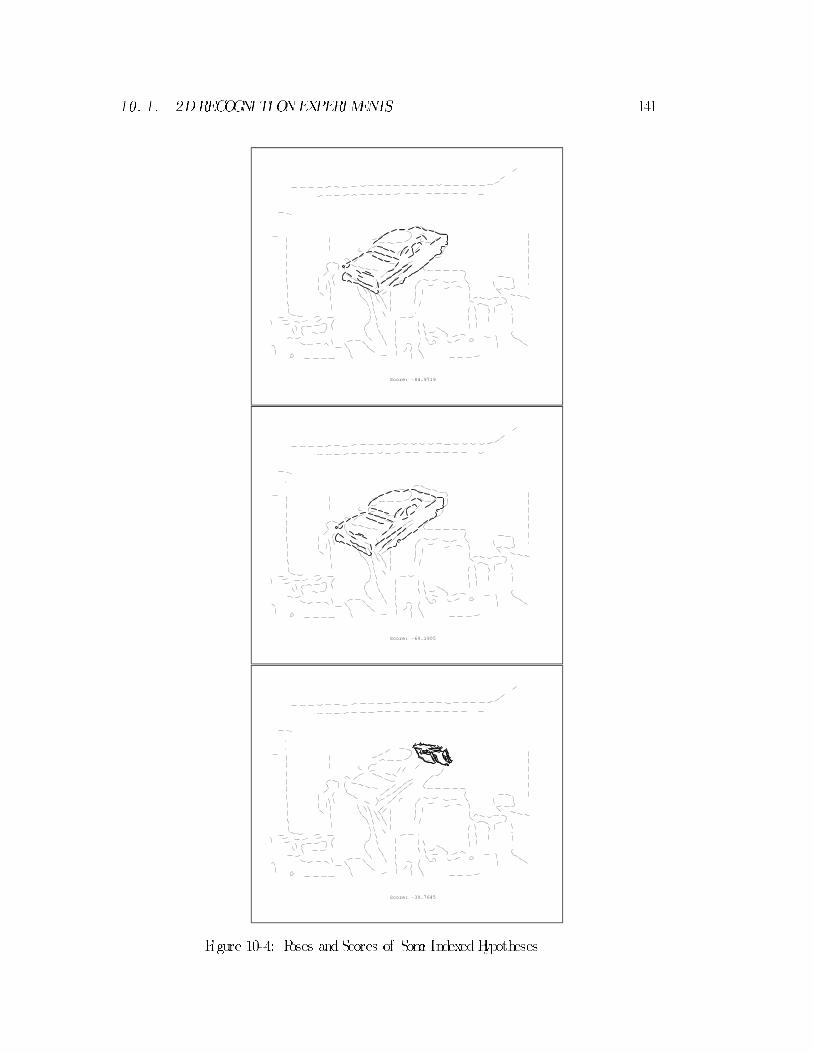
10. 1. 2DRECOGNI TI ONEXPERIMENTS 141
Score: -84.9719
Score: -69.1905
Score: -39.7645
Figure 10-4: Poses andScores of Some IndexedHypotheses

142 CHAPTER10. RECOGNI TI ONEXPERIMENTS
Score: -84.9719
Figure 10-5: Best Al ignment fromIndexer, withCoarse Score
Score: -91.2349
Figure 10-6: Coarse Re�nement, withCoarse Score

10. 1. 2DRECOGNI TI ONEXPERIMENTS 143
Score: -355.069
Figure 10-7: Fine Re�nement, withFine Score
Figure 10-8: Fine Re�nement withVideo Image

144 CHAPTER10. RECOGNI TI ONEXPERIMENTS
Figure 10-9: Correspondences withWeight Larger than .5
and after the re�nement it i s
[1:00166; 0:0051108; 0:68621;�1:7817] T:
The encodingof these poses is describedinSection5.3 (the nul l pose is [1; 0; 0; 0] T . )
The initial pose is in error by about .01 in scale and 5 pixels in position. The �nal
pose errs by about .005 in scale and 1.8 pixels in position. Thus scale accuracy is
improved by a factor of about two, and position accuracy is improved by factor of
about three. Anexperiment showingmore dramatic improvement is describedbelow,
in Section 10.4.1.
In these experiments, less that 15 iterations of the EMalgorithmwere needed for
convergence.
10.1.4 Final EMWeights
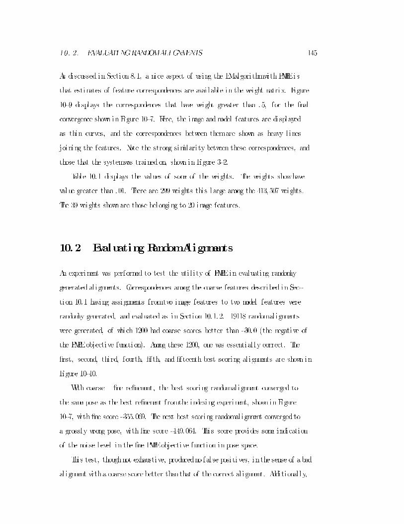
10. 2. EVALUATI NGRANDOMALIGNMENTS 145
As discussed in Section 8.1, a nice aspect of using the EMalgorithmwith PMPEis
that estimates of feature correspondences are avai lable in the weight matrix. Figure
10-9 displays the correspondences that have weight greater than .5, for the �nal
convergence showninFigure 10-7. Here, the image andmodel features are displayed
as thin curves, and the correspondences between themare shown as heavy l ines
joining the features. Note the strong simi lari ty between these correspondences, and
those that the systemwas trained on, shown in Figure 3-2.
Table 10.1 displays the values of some of the weights. The weights showhave
value greater than .01. There are 299 weights this large among the 413,507 weights.
The 39 weights shownare those belonging to 20 image features.
10.2 Evaluating RandomAlignments
An experiment was performed to test the uti l i ty of PMPEin evaluating randomly
generated al ignments. Correspondences among the coarse features described in Sec-
tion 10.1 having assignments fromtwo image features to two model features were
randomly generated, and evaluated as in Section 10.1.2. 19118 randomal ignments
were generated, of which 1200 had coarse scores better than -30.0 (the negative of
the PMPEobjective function). Among these 1200, one was essential ly correct. The
�rst, second, third, fourth, �fth, and �fteenth best scoring al ignments are shown in
Figure 10-10.
With coarse { �ne re�nement, the best scoring randomal ignment converged to
the same pose as the best re�nement fromthe indexing experiment, showninFigure
10-7, with �ne score -355.069. The next best scoring randomal ignment convergedto
a grossly wrong pose, with �ne score -149.064. This score provides some indication
of the noise level in the �ne PMPEobjective function in pose space.
This test, thoughnot exhaustive, producedno false positives, inthe sense of a bad
al ignment witha coarse score better thanthat of the correct al ignment. Additional ly,

146 CHAPTER10. RECOGNI TI ONEXPERIMENTS
Image Index Model Index Weight
90 86 0.022738026840027032
90 101 0.014615921646994348
90 102 0.80796669344409690 103 0.09581539482455806
91 103 0.963344130192666392 85 0.24166197059125494
92 103 0.1977827484742501593 87 0.02784697957543993
93 88 0.37419218245379466
94 87 0.747866772352014295 87 0.4403041327521548696 86 0.6127902576993082
97 85 0.9293665165549775
98 85 0.862176344386899999 84 0.9634827438267516
100 5 0.6499527214931725100 84 0.19705210016850308101 0 0.011400725934573982
101 67 0.9559675939354566102 66 0.9194110795990801102 67 0.0541643593533511103 64 0.04765362703894284
103 65 0.8454128520499249
103 66 0.05787873660955701104 63 0.05270908685541295
104 64 0.8854088356653954104 65 0.014744194821866506
105 62 0.06158503222464117
105 63 0.9139939556525918
106 61 0.09270729594689026106 62 0.8635739185353283
106 63 0.010447389024937672
107 61 0.9108899984969661107 62 0.021204649868405194
108 60 0.861831671427887108 61 0.049220125250993084
109 58 0.018077232316743887
109 59 0.9257311183042934109 60 0.015434004217119308
Table 10.1: Some EMWeights

10. 2. EVALUATI NGRANDOMALIGNMENTS 147
Score: -71.079 Score: -55.6623
Score: -54.6592 Score: -53.6342
Score: -49.4516
Figure 10-10: RandomAlignments

148 CHAPTER10. RECOGNI TI ONEXPERIMENTS
the �ne score of the re�nement of the most promising incorrect randomal ignment
was signi�cantly lower than the �ne score of the (correct) re�ned best al ignment.
10.3 Convergence withOcclusion
The convergence behavior under occlusionof the EMalgorithmwithPMPEwas eval -
uatedusing the coarse features described inSection10.1. Images features simulating
varyingamounts of occlusionwere preparedbyshi ftingavaryingportionof the image.
These images, along with results of coarse { �ne re�nement using the EMalgorithm
are shown inFigure 10-11.
The starting value for the pose was the correct (nul l ) pose. The re�nements
converged to good poses in al l cases, demonstrating that the method can converge
fromgood al ignments withmoderate amounts of occlusion.
The �nal �ne score in the most occluded example is lower than the noise level
observed in the experiment of Section 10.2. This indicates that as the amount of
occlusion increases, a point wi l l be reachedwhere the method wi l l fai l to produce a
goodpose having a score above the noise level . In this experiment it happens before
the method fai l s to converge properly.
10.4 3DRecognitionExperiments
10.4.1 Re�ning3D Alignments
This sectiondemonstrates use of the EMalgorithmwithPMPEto re�ne al ignments
in 3Drecognition. The l inear combinationof views method is used to accommodate
a l imited amount of out of plane rotation. Atwo-viewvariant of LCV, described in
Section 5.5, i s used.
Acoarse { �ne approach was used. Coarse PMPE scores were computed by
smoothingthePMPEobjective function, as describedinSection7.3.2. The smoothing

10. 4. 3DRECOGNI TI ONEXPERIMENTS 149
Score: -338.03 Score: -326.13
Score: -203.142 Score: -163.979
Score: -136.814
Figure 10-11: Fine Convergences withOcclusion

150 CHAPTER10. RECOGNI TI ONEXPERIMENTS
Figure 10-12: Grayscale Image
matrix was
DIAG((7:07) 2; (3:0) 2) :
These numbers are the amounts of additional (arti�cial) variance added for paral lel
andperpendicular deviations, respectively, inthe orientedstationarystatistics model .
The video test image is shown in Figure 10-12. It di�ers fromthe model images
by a signi�cant 3Dtranslation and out of plane rotation. The test image edges are
shown inFigure 10-13.
The object model was derived fromthe twoMeanEdge Images shown in Figure
10-14. These were constructed as described in Section 4.4.
The smoothing used in preparation of the edge maps had 1.93 pixels standard
deviation, and the edge curves were broken arbitrari ly every 10 pixels. Point-radius
features were �tted to the edge curve fragments, as described in Section 5.3, for
purposes of displayandfor computing the orientedstationary statistics, al thoughthe
features usedwithPMPEandthe EMalgorithmwere simplytheXandY coordinates
of the centroids of the curve fragments. Both views of the model features are shown
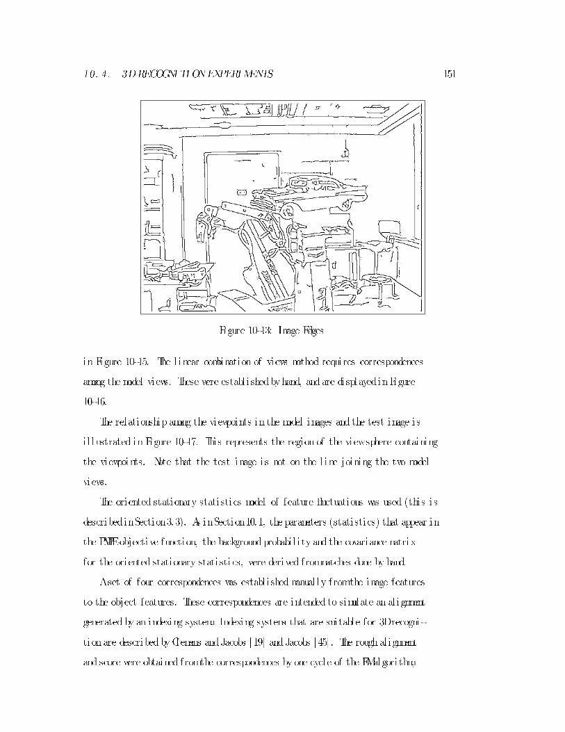
10. 4. 3DRECOGNI TI ONEXPERIMENTS 151
Figure 10-13: Image Edges
in Figure 10-15. The l inear combination of views method requires correspondences
among the model views. These were establ i shedbyhand, andare displayedinFigure
10-16.
The relationshipamong the viewpoints in the model images and the test image is
i l lustrated in Figure 10-17. This represents the region of the viewsphere containing
the viewpoints. Note that the test image is not on the l ine joining the two model
views.
The oriented stationary statistics model of feature uctuations was used (this i s
describedinSection3.3). As inSection10.1, the parameters (statistics) that appear in
the PMPEobjective function, the backgroundprobabi l i ty and the covariance matrix
for the oriented stationary statistics, were derived frommatches done by hand.
Aset of four correspondences was establ i shed manual ly fromthe image features
to the object features. These correspondences are intended to simulate an al ignment
generated by an indexing system. Indexing systems that are suitable for 3Drecogni -
tionare describedbyClemens andJacobs [19] andJacobs [45] . The roughal ignment
and score were obtained fromthe correspondences byone cycle of the EMalgorithm,

152 CHAPTER10. RECOGNI TI ONEXPERIMENTS
Figure 10-14: Model MeanEdge Images

10. 4. 3DRECOGNI TI ONEXPERIMENTS 153
Figure 10-15: Model Features (BothViews)
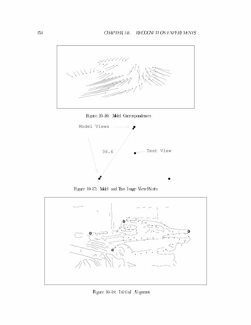
154 CHAPTER10. RECOGNI TI ONEXPERIMENTS
Figure 10-16: Model Correspondences
36.6 Test View
Model Views
Figure 10-17: Model andTest Image ViewPoints
Figure 10-18: Initial Al ignment

10. 4. 3DRECOGNI TI ONEXPERIMENTS 155
Score: -10.8428
Figure 10-19: Coarse Re�nedAl ignment andCoarse Score
Score: -17.2661
Figure 10-20: Fine Re�nedAl ignment andFine Score

156 CHAPTER10. RECOGNI TI ONEXPERIMENTS
Figure 10-21: Fine Re�nedAl ignment withVideo Image
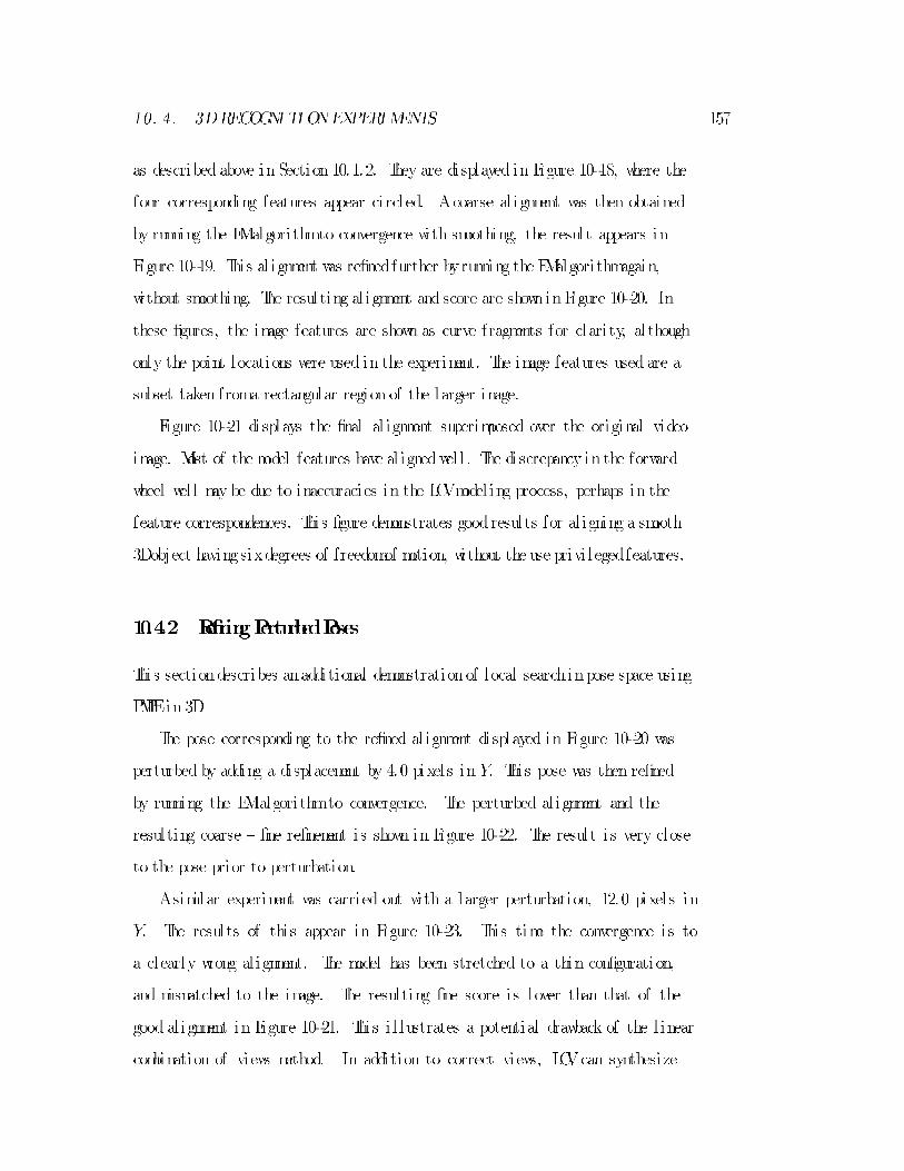
10. 4. 3DRECOGNI TI ONEXPERIMENTS 157
as described above in Section 10.1.2. They are displayed in Figure 10-18, where the
four corresponding features appear circled. Acoarse al ignment was then obtained
by running the EMalgorithmto convergence with smoothing, the result appears in
Figure 10-19. This al ignment was re�nedfurther byrunning the EMalgorithmagain,
without smoothing. The resulting al ignment and score are showninFigure 10-20. In
these �gures, the image features are shown as curve fragments for clari ty, although
only the point locations were used in the experiment. The image features used are a
subset taken froma rectangular region of the larger image.
Figure 10-21 displays the �nal al ignment superimposed over the original video
image. Most of the model features have al ignedwel l . The discrepancy in the forward
wheel wel l may be due to inaccuracies in the LCVmodel ing process, perhaps in the
feature correspondences. This �gure demonstrates goodresults for al igning a smooth
3Dobject havingsixdegrees of freedomof motion, without the use privi legedfeatures.
10.4.2 Re�ningPerturbedPoses
This sectiondescribes anadditional demonstrationof local searchinpose space using
PMPEin 3D.
The pose corresponding to the re�ned al ignment displayed in Figure 10-20 was
perturbed by adding a displacement by 4.0 pixels in Y. This pose was then re�ned
by running the EMalgorithmto convergence. The perturbed al ignment and the
resulting coarse { �ne re�nement is shown in Figure 10-22. The result i s very close
to the pose prior to perturbation.
Asimi lar experiment was carried out with a larger perturbation, 12.0 pixels in
Y. The results of this appear in Figure 10-23. This time the convergence is to
a clearly wrong al ignment. The model has been stretched to a thin con�guration,
and mismatched to the image. The resulting �ne score is lower than that of the
good al ignment in Figure 10-21. This i l lustrates a potential drawback of the l inear
combination of views method. In addition to correct views, LCVcan synthesize
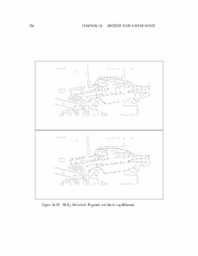
158 CHAPTER10. RECOGNI TI ONEXPERIMENTS
Figure 10-22: Mi ldly PerturbedAl ignment andResulting Re�nement

10. 4. 3DRECOGNI TI ONEXPERIMENTS 159
Score: -15.4685
Figure 10-23: PerturbedAl ignment andResulting Re�nement withFine Score

160 CHAPTER10. RECOGNI TI ONEXPERIMENTS
Score: -11.3126
Figure 10-24: BadAl ignment andResulting Re�nement with Fine Score

10. 4. 3DRECOGNI TI ONEXPERIMENTS 161
views where the model i s stretched. LCV, as used here, has 8 parameters, rather
than the 6 of rigidmotion. The two extra parameters determine the stretching part
of the transformation. This problemcan be addressed by checking, or enforcing, a
quadratic constraint on the parameters. This i s discussed in [71] .
Another simi lar experiment was performed starting with a very bad al ignment.
The results appear in Figure 10-24. The algorithmwas able to bring some features
into al ignment, but the score remained low.

162 CHAPTER10. RECOGNI TI ONEXPERIMENTS

Chapt er 11
Concl us i ons
Visual object recognition { �nding a known object in scenes, where the object i s
smooth, i s viewedunder varying i l lumination conditions, has six degrees of freedom
of position, i s subject to occlusions and appears against varying backgrounds { sti l l
presents problems. In this thesis, progress has been made by applying methods of
statistical inference to recognition. Ever-present uncertainties are accommodated
by statistical characterizations of the recognition problem: MAPModel Matching
(MMM) and Posterior Marginal Pose Estimation (PMPE). MMMwas shown to be
e�ective for searchingamong feature correspondences andPMPEwas showne�ective
for searches inpose space. The issue of acquiring sal ient object features under varying
i l luminationwas addressed by using MeanEdge Images.
The al ignment approach, which leverages fast indexing methods of hypothesis
generation, i s uti l i zed. Angle Pair Indexing is introduced as an e�cient 2Dindexing
method that does not depend on extended or special features that can be hard to
detect. An extension to the al ignment approach that may be summarized as al i gn
re�ne veri f y i s advocated. The EMalgorithmis employedfor re�ning the estimate of
the object' s pose whi le simultaneously identi fying and incorporating the constraints
of al l supporting image features.
Areas for future research include the fol lowing:
163

164 CHAPTER11. CONCLUSI ONS
� Indexingwas not usedinthe 3Drecognitionexperiments. Identi fying a suitable
mechanismfor this purpose that meshes wel l withthe type of features usedhere,
wouldbe an improvement.
� Too fewviews were used in model construction. Ful ly automating the model
acquisi tionprocess, as described inChapter 4, andacquiring models frommore
views wouldhelp.
� Extending the formulations of recognitiontohandle multiple objects i s straight-
forward, but identi fying suitable search strategies i s an important and non-
trivial task.
� Incorporating non-l inear models of projection into the formulationwouldal low
robust performance in domains having serious perspective distortions.
� Using image-l ike tables couldspeedthe evaluationof the PMPEobjective func-
tion.
� Investigating the use of PMPEin object tracking or in other active vision do-
mains might prove fruitful .
More work in these areas wi l l lead to practical and robust object recognition
systems.

Appendi x A
165

166 APPENDIXA. NOTATION
Not at i on
Symbol Meani ng De�ni ng Sect i on
Y=fY 1; Y2; : : : ; Yng the image 2.1
n number of image features
Yi 2R v image feature 2.1
M=fM 1;M2; : : : ;Mmg the object model 2.1
m number of object features
Mj model feature, frequentlyM j 2R v�z 2.1
? the background feature 2.1
�=f� 1;�2; : : : ;�ng correspondences 2.1
�i 2M[f?g assignment of image feature i 2.1
�2R z pose of object 5.1
P(M j; �) projection into image 5.1
G (x) Gaussian probabi l i ty density 3.2 6.1
i j covariance matrix of feature pair 3.3
stationary feature covariance matrix 3.3
� covariance matrix of pose prior 6.1
B; B i backgroundprobabi l i ty 2.2 2.4
Wk extent of image feature dimension k 3.1
�i j; � correspondence reward 6.1
x estimate of x
p(� ) probabi l i ty (see below)
Probabi l i ty notation is somewhat abused in this work, in the interest of brevity.
p(x) maystandfor either a probabi l i tymass functionof a discrete variable x, or for a
probabi l i tydensity function of a continuous variable x. The meaning wi l l be clear in

167
context basedonthe type of the variable argument. Additional ly, mixedprobabi l i ties
are describedwith the same notation. For example p(�; �j Y) stands for the mixed
probabi l i ty function that is a probabi l i ty mass function of � (the discrete variable
describing correspondences), anda probabi l i tydensity functionof �(the pose vector)
{ both conditioned onY (the image feature coordinates).

168 APPENDIXA. NOTATION

Bi bl i ogr aphy
[1] N. Ayache and O.D. Faugeras. HYPER: ANewApproach for the Recognition
andPositioning of Two-Dimensional Objects. IEEETransact i ons PAMI, PAMI-
8(1):44{54, January 1986.
[2] S.T. Barnard. Stereo Matching by Hierarchical , Microcanonical Anneal ing. In
Proceedi ngs of the Tenth Internat i onal Joi nt Conf erence onArt i �ci al Intel l i gence,
pages 832{835, August 1987.
[3] H.G. Barrow, J.M. Tenenbaum, R.C. Bol les, andH.C. Wolf. Parametric Corre-
spondence and Chamfer Matching: Two NewTechniques for Image Matching.
InProc. 5th Int . Joi nt Conf . Art i �ci al Intel l i gence, pages 659{663, 1977.
[4] J.V. Beck andK.J. Arnold. Parameter Est imat i on i n Sci ence and Engi neeri ng.
JohnWiley & Sons, 1977.
[5] P.J. Besl and R.C. Jain. Three-Dimensional Object Recognition. Comput i ng
Surveys, 17:75{145, 1985.
[6] J. Beveridge, R. Weiss, and E. Riseman. Optimization of 2-Dimensional Model
Matching. InProceedi ngs: Image Understandi ng Workshop, pages 815{830. Mor-
ganKaufmann, 1989.
[7] A. Blake andA. Zisserman. Vi sual Reconst ruct i on. MITPress, 1987.
169
170 BI BLI OGRAPHY
[8] G. Borgefors. Hierarchical Chamfer Matching: AParametric Edge Matching
Algorithm. IEEETransact i ons PAMI, 10(6):849{865, November 1988.
[9] T.M. Breuel . Geometri c Aspect s of Vi sual Object Recogni t i on. PhDthesis, MIT
Department of Brain andCognitive Sciences, 1992.
[10] R.A. Brooks. Model -Based Three-Dimensional Interpretations of Two-
Dimensional Images. IEEE Transact i ons PAMI, PAMI-5(2):140 { 150, March
1983.
[11] J.B. Burns. Matchi ng 2DImages to Mul t i pl e 3DObj ect s Usi ng Vi ew Descri p-
t i on Networks. PhDthesis, Universi ty of Massachusetts at Amherst, Dept. of
Computer and Information Science, 1992.
[12] J.B. Burns and E.M. Riseman. Matching Complex Images to Multiple 3DOb-
jects Using ViewDescription Networks. In Proceedi ngs: Image Understandi ng
Workshop, pages 675{682. MorganKaufmann, January 1992.
[13] J.F. Canny. AComputational Approachto Edge Detection. IEEETransact i ons
PAMI, PAMI-8(6):679{698, November 1986.
[14] T.A. Cass. ARobust Paral lel Implementation of 2DModel -BasedRecognition.
In Proceedi ngs of the Computer Soci ety Conf erence on Computer Vi si on and
Pat t ern Recogni t i on, pages 879{884. IEEE, June 1988.
[15] T.A. Cass. Pol ynomi al -Time Geometri c Matchi ng f or Obj ect Recogni t i on. PhD
thesis, MITDepartment Electrical Engineering andComputer Science, 1992.
[16] T.A. Cass. Polynomial -Time Object Recognition in the Presence of Clutter,
Occlusion, and Uncertainty. In G. Sandini , editor, Computer Vi si on { ECCV
'92, pages 834{851. Springer Verlag, 1992.

BI BLI OGRAPHY 171
[17] P. Cheeseman. AMethodof ComputingGeneral izedBayesianProbabi l i tyValues
for Expert Systems. InProc. Ei ghth Int . Joi nt Conf . Art i �ci al Intel l i gence, pages
198{202, 1983.
[18] R.T. ChinandC.R. Dyer. Model -BasedRecognitioninRobot Vision. Comput i ng
Surveys, 18:67{108, 1986.
[19] D.T. Clemens and D.W. Jacobs. Model Group Indexing for Recognition. In
Symposi umon Advances i n Intel l i gent Syst ems. SPIE, 1990.
[20] D.T. Clemens andD.W. Jacobs. Space andTimeBounds onIndexing3-DModels
from2-DImages. IEEETransact i ons PAMI, 13(10):1007{1017, October 1991.
[21] A.P. Dempster, N.M. Laird, andD.B. Rubin. MaximumLikel ihoodfromIncom-
plete Data via the EMAlgorithm. J. Roy. Stat i st . Soc. , 39:1 { 38, 1977.
[22] R.O. Duda and P.E. Hart. Pat tern Cl assi �cat i on and Scene Anal ysi s. John
Wiley andSons, 1973.
[23] P. Dykstra and M.J. Muuss. The BRLCADPackage: an Overview. In Pro-
ceedi ngs of the Fourth USENIX Computer Graphi cs Workshop, pages 73{80,
Cambridge MA, 1987.
[24] S. Edelman and T. Poggio. Bringing the Grandmother Back Into the Picture:
a Memory-Based Viewof Object Recognition. A.I. Memo 1181, Massachusetts
Insti tute of Technology, Apri l 1990.
[25] D.I. Perrett et al . Visual Cel l s in the Temporal Cortex Sensitive to Face View
andGaze Control . Proc. Roy. Soc. London B, 223:293 { 317, 1985.
[26] P. FuaandA.J. Hanson. Objective Functions for Feature Discrimination: Appl i -
cations to Semiautomated and Automated Feature Extraction. InProceedi ngs:
Image Understandi ng Workshop, pages 676{694. MorganKaufmann, 1989.
172 BI BLI OGRAPHY
[27] P. Fua andA.J. Hanson. Objective Functions for Feature Discrimination: The-
ory. In Proceedi ngs: Image Understandi ng Workshop, pages 443{459. Morgan
Kaufmann, 1989.
[28] S. Geman and D. Geman. Stochastic Relaxation, Gibbs Distributions, and the
BayesianRestorationof Images. IEEETransact i ons PAMI, PAMI-6(6):721{741,
November 1984.
[29] C. Goad. Fast 3-DModel BasedVision. InAlexP. Pentland, editor, FromPi xel s
to Predi cates, pages 371{391. Ablex Publ ishing Co. , 1986.
[30] S. A. Goldman. E�cient Methods for Calculating MaximumEntropyDistribu-
tions. Technical Report TR-391, MITLaboratory for Computer Science, 1987.
[31] T.J. Green, Jr. Three-Dimensi onal Obj ect Recogni t i on Usi ng Laser Radar. PhD
thesis, MITDepartment Electrical Engineering andComputer Science, 1992.
[32] T.J. Green, Jr. and J.H. Shapiro. Maximum-Likel ihood Laser Radar Range
Pro�l ingwiththe Expectation{MaximizationAlgorithm. Opt . Eng. , November
1992.
[33] W.E.L. Grimson. Computational Experiments with a Feature Based Stereo Al-
gorithm. IEEETransact i ons PAMI, PAMI-7(1):17{34, January 1985.
[34] W.E.L. Grimson. Obj ect Recogni t i on by Computer: The Rol e of Geometri c Con-
st rai nt s. MITPress, 1990.
[35] W.E.L. Grimson and D.P. Huttenlocher. On the Veri�cation of Hypothesized
Matches inModel -BasedRecognition. InFi rst Europ. Conf . Comp. Vi si on, pages
489{498, 1990.
[36] W.E.L. GrimsonandT. Lozano-P�erez. Local izing OverlappingParts bySearch-
ing the InterpretationTree. IEEETransact i ons PAMI, PAMI-9(4):469{482, July
1987.

BI BLI OGRAPHY 173
[37] R.M. Haral ick. Digital Step Edges fromZero Crossing of Second Directional
Derivatives. IEEETransact i ons PAMI, PAMI-6(1):58 { 129, January 1984.
[38] R.M. Haral ick, H.Joo, C.N.Lee, X.Zhuang, V.G.Vaidya, and M.B.Kim. Pose
Estimation fromCorresponding Point Data. IEEETrans. on Systems Man and
Cybernet i cs, 19(6):1426 { 1445, December 1989.
[39] B.K.P. Horn. Robot Vi si on. McGraw-Hi l l , NewYork, 1986.
[40] P.V.C. Hough. Methods and Means for Recognizing Complex Patterns. U.S.
Patent 3069654, 1962.
[41] P.J. Huber. Robust Stat i st i cs. J. Wiley &Sons, 1981.
[42] D.P. Huttenlocher, K. Kedem, K. Sharir, and M. Sharir. The Upper Envelope
of Voronoi Surfaces and its Appl ications. In Proceedi ngs of the Seventh ACM
Symposi umon Computat i onal Geometry, pages 194{293, 1991.
[43] D.P. Huttenlocher and S. Ul lman. Recognizing Sol idObjects by Al ignment. In
Proceedi ngs: Image Understandi ng Workshop, pages 1114{1124. Morgan Kauf-
mann, Apri l 1988.
[44] J. Il l ingworth and J. Kittler. ASurvey of the Hough Transform. Computer
Vi si on, Graphi cs, and Image Processi ng, 44:87{116, 1988.
[45] D.W. Jacobs. Recogni zi ng 3DObj ect s Usi ng 2DImages. PhDthesis, MITDe-
partment Electrical Engineering andComputer Science, 1992.
[46] E. T. Jaynes. Where Do We Go FromHere? In C. R. Smith and W. T.
Grandy, Jr. , editors, Maximum-Entropy and Bayesi an Methods i n Inverse Prob-
l ems, pages 21 { 58. MITPress, 1982.
[47] H. Jiang, R.A. Robb, andK.S. Holton. ANewApproach to 3-DRegistrationof
Multimodal i tyMedical Images bySurfaceMatching. InVi sual i zat i on i n Bi omed-
i cal Comput i ng, pages 196{213. SPIE, 1992.

174 BI BLI OGRAPHY
[48] R. Kumar and A.R. Hanson. Robust Estimation of Camera Location and Ori -
entation fromNoisy Data Having Outl iers. InProc. of the Workshop on Inter-
pretat i on of 3DScenes, pages 52{60. IEEEComputer Society, 1989.
[49] Y. Lamdan and H.J. Wolfson. Geometric Hashing: AGeneral and E�cient
Model -BasedRecognition Scheme. In Second Int . Conf . Comp. Vi si on, 1988.
[50] P. Lipson. Model Guided Correspondence. Master' s thesis, MITDepartment
Electrical Engineering andComputer Science, 1992.
[51] D.G. Lowe. Perceptual Organi zat i on and Vi sual Recogni t i on. Kluwer Academic
Publ ishers, 1985.
[52] D. Marr. Vi si on. Freeman, 1982.
[53] D. Marr andE. Hi ldreth. Theory of Edge Detection. Proc. Roy. Soc. London B,
207:187 { 217, 1980.
[54] J.L. Marroquin. Probabi l i st i c Sol ut i on of Inverse Probl ems. PhDthesis, MIT
Department Electrical Engineering andComputer Science, 1985.
[55] J.L. Marroquin, S. Mitter, and T. Poggio. Probabi l i stic Solution of Il l -posed
Problems inComputational Vision. Journal of the Am. Stat . Assoc. , 82(397):76{
89, 1987.
[56] M. Menon andW.M. Wel ls III. Massively Paral lel Image Restoration. InPro-
ceedi ngs of the Internat i onal Joi nt Conf erence on Neural Networks, San Diego,
CA., 1990. IEEE.
[57] D. Mercer. Opt imi zat i on of a Curvature-Gradi ent Dot -Product Li ne and Edge
Detector. Bachelor' s Thesis, MITDepartment of Electrical Engineering and
Computer Science, 1991.

BI BLI OGRAPHY 175
[58] J. Ponce andD.J. Kriegman. OnRecognizingandPositioningCurved3DObjects
FromImage Contours. In Image Understandi ng Workshop (Pal o Al to, CA, May
23-26, 1989), pages 461{470, 1989.
[59] W.H. Press, B.P. Flannery, S.A. Teukolsky, and W.T. Vetterl ing. Numeri cal
Reci pes: the Art of Sci ent i �c Comput i ng. Cambridge Universi ty Press, 1986.
[60] E. Rivl in and R. Basri . Local ization and Positioning Using Combinations of
Model Views. Technical Report CAR-TR-631, Center for AutomationResearch,
Universi ty of Maryland, 1992.
[61] T.J. Sejnowski andC.R. Rosenberg. Paral lel Networks that Learnto Pronounce
Engl i sh Text. Compl ex Systems, 1:145{168, 1987.
[62] J.H. Shapiro, R.W. Reinhold, and D. Park. Performance Analyses for Peak-
Detecting Laser Radars. Proceedi ngs of the SPIE, 663:38{56, 1986.
[63] J.H. Shapiro andA.L. Wil l sky. Stochastic Processes, Detection, andEstimation.
MITCourse 6.432 SupplementaryNotes.
[64] S.C. Shapiro, editor. Encycl opedi a of Art i �ci al Intel l i gence. JohnWiley&Sons,
1987.
[65] A. Shashua. Correspondence and A�ne Shape fromtwo Orthographic Views:
MotionandRecognition. A.I. Memo1327, Massachusetts Insti tute of Technology,
December 1991.
[66] A. Shashua and S. Ul lman. Structural Sal iency: The Detection of Global ly
Sal ient Structures Using a Local ly Connected Network. In Proceedi ngs of the
2nd Internat i onal Conf erence on Computer Vi si on, pages 321{327, 1988.
[67] R.S. Stephens. AProbabi l i stic Approach to the Hough Transform. InProceed-
i ngs of the Bri t i sh Machi ne Vi si on Conf erence, pages 55{60, Univ. of Oxford,
September 1990.
176 BI BLI OGRAPHY
[68] R.S. Stephens. The Hough Transf orm: AProbabi l i st i c Approach. PhDthesis,
Cambridge Universi ty, Department of Engineering, 1990.
[69] R.W. Taylor andA.P. Reeves. Classi�cationQual i ty Assessment for a General -
izedModel -BasedObject Identi�cationSystem. IEEETransact i ons on Systems,
Man, and Cybernet i cs, 19:861{866, 1989.
[70] D.W. Thompson and J.L. Mundy. Three Dimensional Model Matching From
anUnconstrainedViewpoint. InProceedi ngs IEEEInternat i onal Conf erence on
Robot i cs and Automat i on, pages 208 { 219. IEEE, 1987.
[71] S. Ul lman and R. Basri . Recognition by Linear Combinations of Models. A.I.
Memo 1152, Massachusetts Insti tute of Technology, August 1989.
[72] H.L. Van Trees. Detect i on, Est imat i on, and Modul at i on Theory, part 1. John
Wiley andSons, 1968.
[73] G.H. Wannier. El ements of Sol i d State Theory. Cambridge Universi ty Press,
1959.
[74] W.M. Wel ls III. AStatistical Approach to Model Matching. In Symposi umon
Advances i n Intel l i gent Syst ems. SPIE, 1990.
[75] W.M. Wel ls III. MAPModel Matching. In Proceedi ngs of the Computer So-
ci ety Conf erence on Computer Vi si on and Pat t ern Recogni t i on, pages 486{492,
Lahaina, Maui , Hawai i , June 1991. IEEE.
[76] W.M. Wel ls III. Posterior Marginal Pose Estimation. In Proceedi ngs: Image
Understandi ng Workshop, pages 745 { 751. MorganKaufmann, January 1992.
[77] C.F.J. Wu. On the Convergence Properties of the EMAlgorighm. The Annal s
of Stat i st i cs, 11(1):95 { 103, 1983.

BI BLI OGRAPHY 177
[78] A. Yui l le, D. Geiger, andH. B�ultho�. Stereo Integration, MeanFieldTheoryand
Psychophysics. InComputer Vi si on { ECCV90, pages 73{82. Springer Verlag,
1990.
[79] A.L. Yui l le. General izedDeformable Models, Statistical Physics, andMatching
Problems. Neural Computat i on, 2:1 { 24, 1990.


