Wireless Communication Technologies (16:332:546)
Taught by Professor Narayan Mandayam
Lecture 7 : Co-Channel
Interference
Slides prepared by : Shuangyu Luo

Co-channel interference
4 Examples of CCI, and channel reuse
Mobile channel fading effects
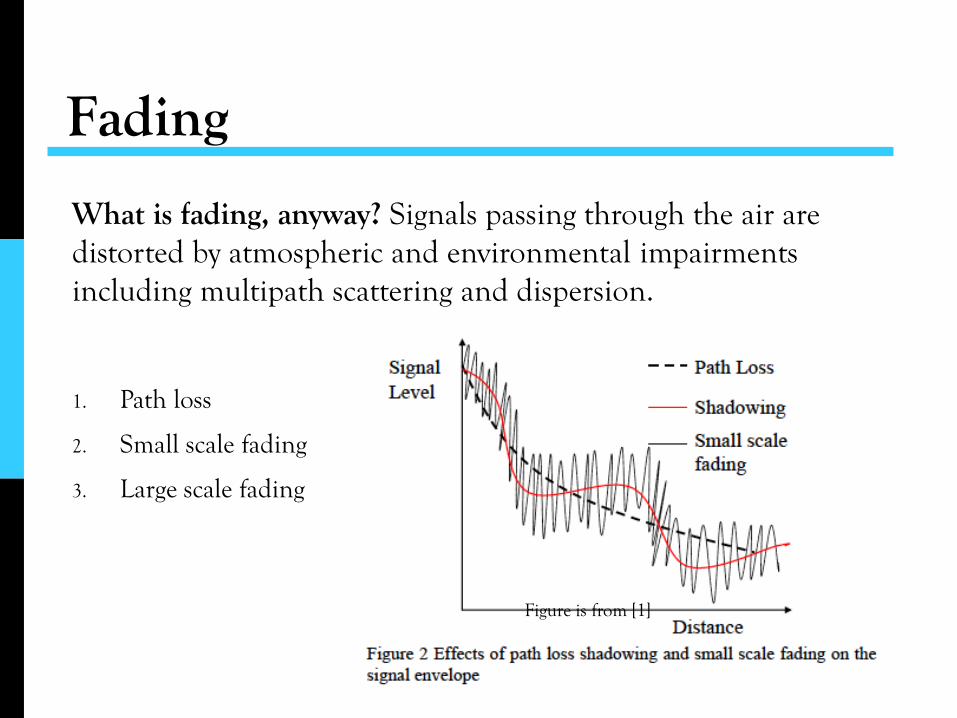
1. Path Loss
2. Small Scale Fading
3. Large Scale Fading (Shadowing)
4. Rayleigh, Rician, Suzuki fading model
Multiple lognormal interference
Three approximation methods
Probability of outage
Outline
What is co-channel interference? 1. Co-channel interference is one channel
creates an undesired effect in another
channel
2. Co-channel interference is cross talk
from two different radio transmitters
using the same frequency.
Example1 of co-channel interference
Why we need to use the same frequency?
That’s because in wireless communication
systems, we only have limited spectrum
resource, the same frequency channels are
used many times, this is called “channel re-
use”.

Example1 of co-channel interference 1. In cellular mobile communication system, available
frequency spectrum is limited, they are divided into non-
overlapping spectrum bands and assigned to different cells.
2. A cell is a hexagonal area around the base station antenna,
it will share the same frequency with different cells.
3. These cells transmit signals using the same frequency
4. Signals at the same frequencies arrive at the receiver from
the undesired transmitters located far away in some other
cells
5. Co-channel interference will deteriorate the receiver
performance. [6]
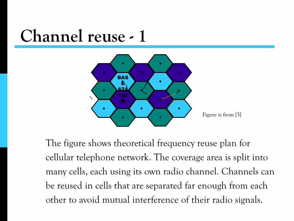
The figure shows theoretical frequency reuse plan for
cellular telephone network. The coverage area is split into
many cells, each using its own radio channel. Channels can
be reused in cells that are separated far enough from each
other to avoid mutual interference of their radio signals.
Channel reuse - 1
BAS
E
STA
TIO
N
Figure is from [3]
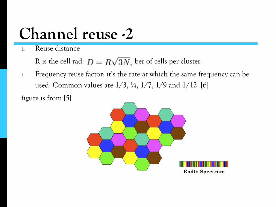
Channel reuse -2 1. Reuse distance
R is the cell radius, N is the number of cells per cluster.
1. Frequency reuse factor: it’s the rate at which the same frequency can be
used. Common values are 1/3, ¼, 1/7, 1/9 and 1/12. [6]
figure is from [5]
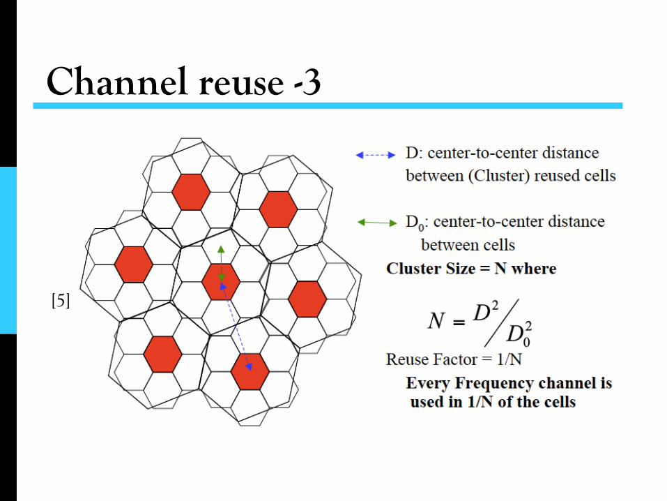
Channel reuse -3
[5]
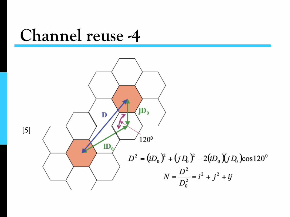
Channel reuse -4
[5]

Channel reuse -5
[5]
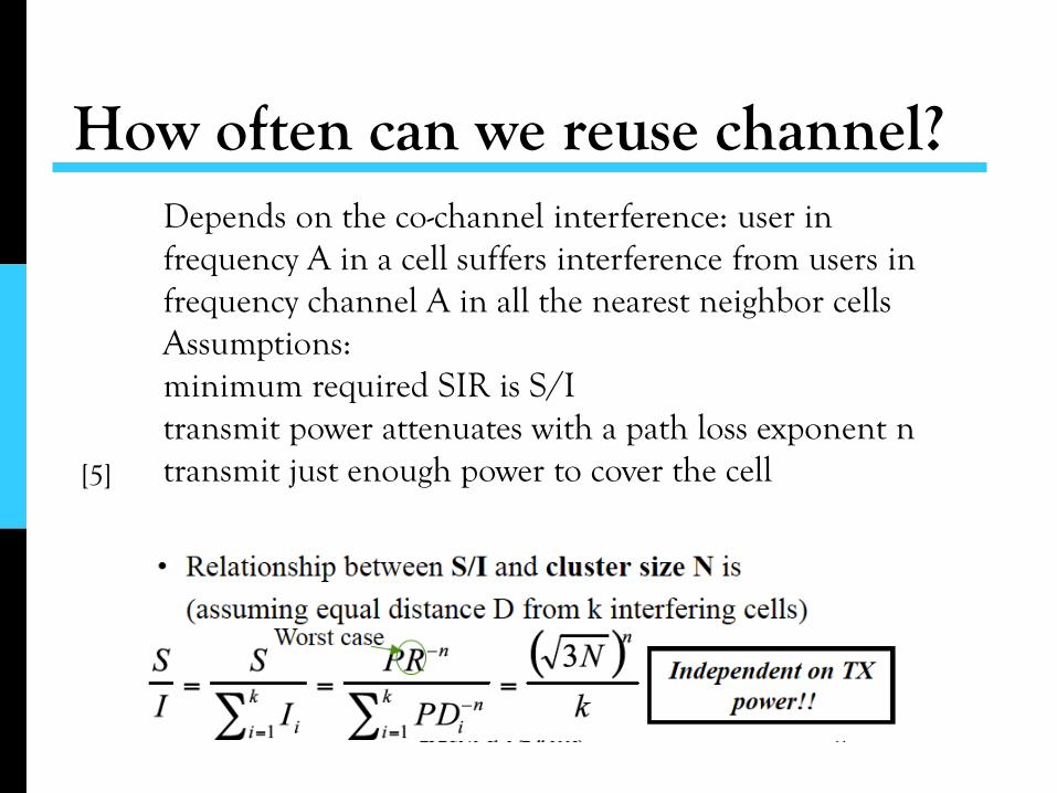
How often can we reuse channel?
[5]
Depends on the co-channel interference: user in frequency A in a cell suffers interference from users in frequency channel A in all the nearest neighbor cells Assumptions: minimum required SIR is S/I transmit power attenuates with a path loss exponent n transmit just enough power to cover the cell
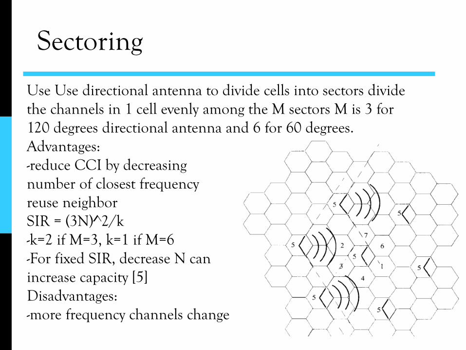
Sectoring
Use Use directional antenna to divide cells into sectors divide the channels in 1 cell evenly among the M sectors M is 3 for 120 degrees directional antenna and 6 for 60 degrees. Advantages: -reduce CCI by decreasing number of closest frequency reuse neighbor SIR = (3N)^2/k -k=2 if M=3, k=1 if M=6 -For fixed SIR, decrease N can increase capacity [5] Disadvantages: -more frequency channels change
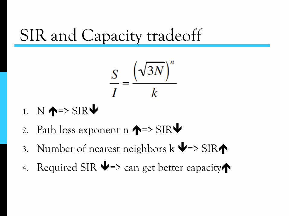
SIR and Capacity tradeoff
1. N => SIR
2. Path loss exponent n => SIR
3. Number of nearest neighbors k => SIR
4. Required SIR => can get better capacity
Example2 of co-channel interference
1. Adverse weather condition: During periods of
abnormally high-pressure weather, VHF signals
which would normally exit through the atmosphere
can instead be reflected by the troposphere. This
tropospheric ducting will cause the signal to travel
much further than intended; often causing
interference to local transmitters in the areas
affected by the increased range of the distant
transmitter. [6]
1. Poor frequency planning: Poor planning of
frequencies by broadcasters can cause CCI. Once
in a town, its television transmitter system use the
same frequencies as the town next to it, but with
opposite polarization. Both transmitters can be
picked up causing heavy CCI. The problem forces
residents to use alternative transmitters to receive
TV programming. [6]
Example3 of co-channel interference
Overly-crowded radio spectrum
1. In many populated areas, there is just no enough
room in the radio spectrum. The stations will
receive two, three or more stations on the same
frequency at once. [6]
Example4 of co-channel interference

Adjacent-channel interference
Adjacent-channel interference or ACI is interference caused by extraneous power from a signal in an adjacent channel. ACI may be caused by inadequate filtering, such as incomplete filtering of unwanted modulation products in frequency modulation (FM) systems, improper tuning, or poor frequency control, in either the reference channel or the interfering channel, or both. ACI is distinguished from crosstalk.[6]
1. Path loss
2. Small scale fading
3. Large scale fading
Fading
Figure is from [1]
What is fading, anyway? Signals passing through the air are distorted by atmospheric and environmental impairments including multipath scattering and dispersion.
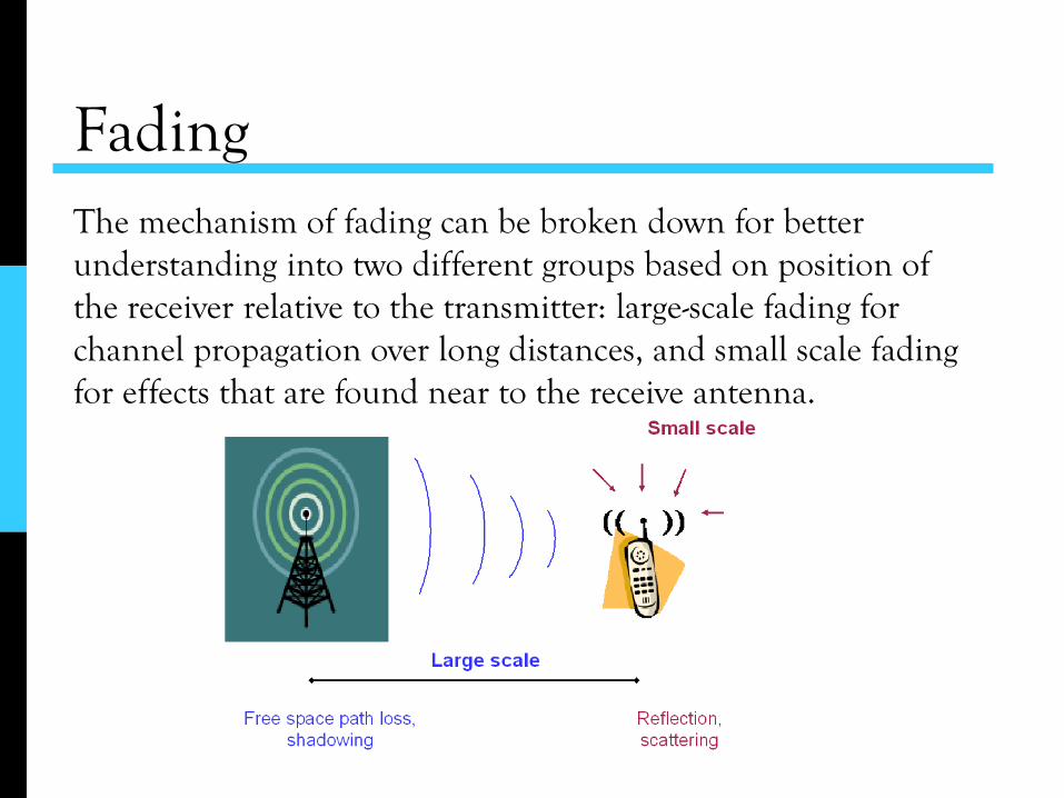
Fading The mechanism of fading can be broken down for better understanding into two different groups based on position of the receiver relative to the transmitter: large-scale fading for channel propagation over long distances, and small scale fading for effects that are found near to the receive antenna.

Path Loss Path loss: attenuation of wave as it propagates through space. Path loss may be due to many effects, such as free-space loss, refraction, diffraction, reflection, aperture-medium coupling loss, and absorption. Path loss is also influenced by terrain contours, environment (urban or rural, vegetation and foliage), propagation medium (dry or moist air), the distance between the transmitter and the receiver, and the height and location of antennas.
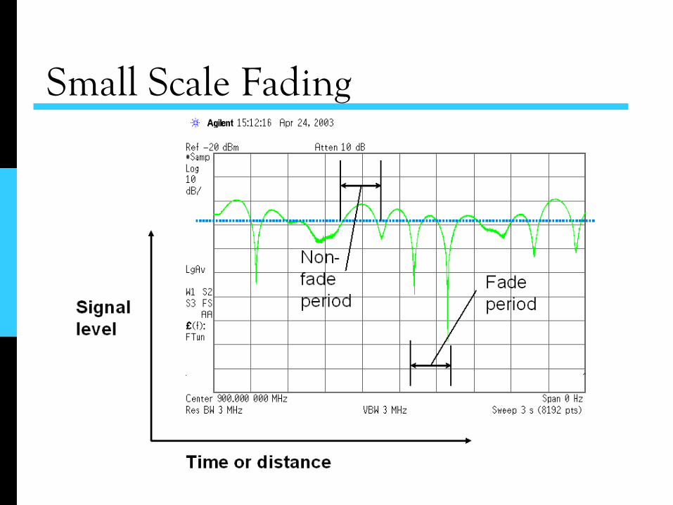
Small Scale Fading

Large Scale Fading 1. Large scale fading is an average path loss with wide peaks and troughs
caused by shadowing
Rayleigh fading The Rayleigh distribution is a good model for channel
propagation when there is no strong line of sight path from
transmitter to receiver. This can represent the channel
conditions seen on a busy street in a city, where the base
station is hidden behind a building several blocks away and
the arriving signal is bouncing off many scattering objects in
the local area.

Rician Fading Rayleigh fading is considered a worst case scenario. In rural environments, where the multipath profile includes a few reflected paths combined with a strong line of sight path, the spectral power follows a Rician distribution. The angle of arrival of the direct ray, as well as the ratio of the power between the direct ray and the mulipath rays, determine how much effect the energy from the direct path has on the normal Rayleigh model.[7]
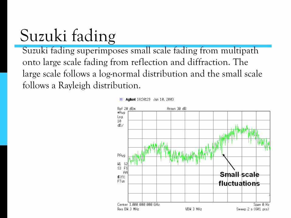
Suzuki fading Suzuki fading superimposes small scale fading from multipath onto large scale fading from reflection and diffraction. The large scale follows a log-normal distribution and the small scale follows a Rayleigh distribution.

Lognormal random variable In probability and statistics, the log-normal distribution is the single-tailed probability distribution of any random variable whose logarithm is normally distributed. If X is a random variable with a normal distribution, then Y = exp(X) has a log-normal distribution; likewise, if Y is log-normally distributed, then ln(Y ) is normally distributed. [2]
Given X, a Gaussian random variable with mean and variance , is a lognormal random variable (RV) with probability density function (PDF):
Figure is from [2]
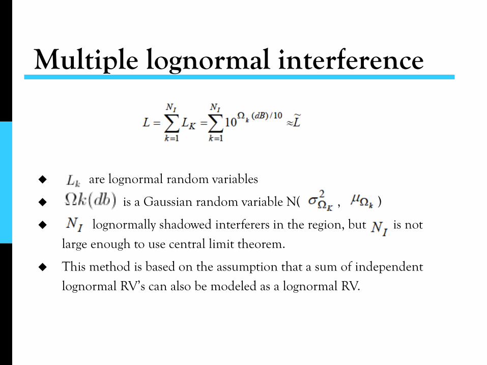
are lognormal random variables
is a Gaussian random variable N( , )
lognormally shadowed interferers in the region, but is not
large enough to use central limit theorem.
This method is based on the assumption that a sum of independent
lognormal RV’s can also be modeled as a lognormal RV.
Multiple lognormal interference
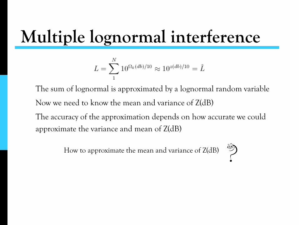
The sum of lognormal is approximated by a lognormal random variable
Now we need to know the mean and variance of Z(dB)
The accuracy of the approximation depends on how accurate we could
approximate the variance and mean of Z(dB)
Multiple lognormal interference
How to approximate the mean and variance of Z(dB)

Three approximation methods How to approximate the mean and variance of Z(dB)
Next we introduce the most well known approaches:
1. Fenton-Wilkinson method
2. Schwartz Yeh’s method
3. Farley’s method
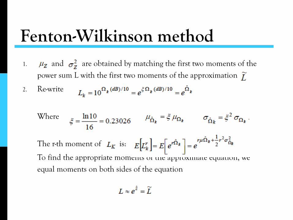
1. and are obtained by matching the first two moments of the
power sum L with the first two moments of the approximation
2. Re-write
Where
The r-th moment of is:
To find the appropriate moments of the approximate equation, we
equal moments on both sides of the equation
Fenton-Wilkinson method

Fenton-Wilkinson method
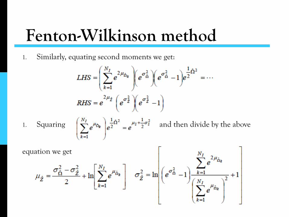
1. Similarly, equating second moments we get:
1. Squaring and then divide by the above
equation we get
Fenton-Wilkinson method

Fenton-Wilkinson method
Note:
The moments itself may not match exactly, but the approximation
works well evaluating the probability

1. Equates LHS and RHS in Fenton Wilknson method by evaluating the
exact expression for the first two moments of the sum of two lognormal
RVs. [1]
2. Recursion is then used to evaluate for general number of interferers.
Schwarz Yeh’s method

The exact expressions for 1st and 2nd moments of the RV Z were derived. By again assuming that the sum of two lognormal RV's is a lognormal RV.
A recursive technique was developed for computing the 1st two moments of a sum M > 2 independent lognormal RVs.
In [4], it is proved that Wilkinson's approach is preferred over Schwartz-Yeh 's approach.
Wilkinsons approach is easier to use than Schwartz and Yehs approach, especially for M > 2 cases, since to use the latter method one has to recursively use relatively complex expressions to compute the 1st two moments of , and for values of the CDF less than 0.1, Wilkinsons approach gives more accurate results.[2]
Schwarz Yeh’s method

Farley’s method
1. Let X1, …, XM be M independent and identically distributed Gaussian
RVs. The Farley’s approximation is:
2. Farley’s method is valid for large variances. It is a strict lower bound on
the CDF for any variance.[2]
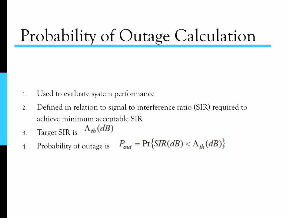
Probability of Outage Calculation
1. Used to evaluate system performance
2. Defined in relation to signal to interference ratio (SIR) required to
achieve minimum acceptable SIR
3. Target SIR is
4. Probability of outage is

Signal to Interference Ratio:
is the desired signal’s power. The signal has LOS components and
therefore affected by Ricean fading. is the interfering signal power
of the BS. The co-channel BS signal undergo Raleigh Fading
because of non-LOS components. has non-central chi-square
distribution and has exponential distribution.
SIR
S0
Sk
K th
S0
Sk
Probability of outage
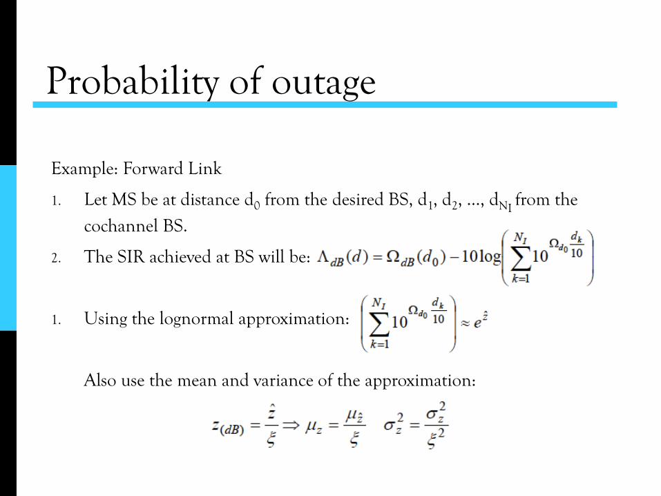
Example: Forward Link
1. Let MS be at distance d0 from the desired BS, d1, d2, …, dNI from the
cochannel BS.
2. The SIR achieved at BS will be:
1. Using the lognormal approximation:
Also use the mean and variance of the approximation:
Probability of outage
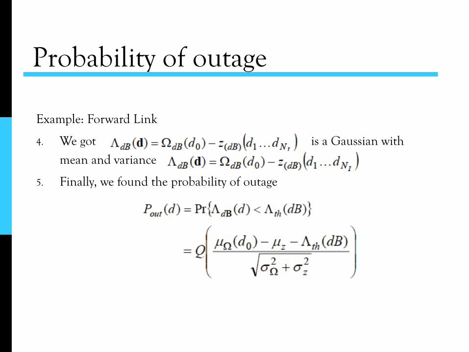
Example: Forward Link
4. We got is a Gaussian with
mean and variance
5. Finally, we found the probability of outage
References [1] http://www.winlab.rutgers.edu/~narayan/Course/Wless/559_5.html [2] http://etd.ohiolink.edu/view.cgi/Li%20Xue.pdf?wright1229358144 [3] http://www.cs.jhu.edu/~baruch
[4] Beaulieu, N.C., Abu-Dayya, A.A. and McLane, P.J., \Comparison of methods of computing lognormal sum distributions and outages for digital wireless applications", Communications,1994. ICC '94, SUPERCOMM/ICC '94, Conference Record, vol.3, pp. 1270-1275, May 1994.
[5] Lecture notes from ECE course taught by Prof. Shu-Kwan Cheng in Hong Kong University of science and technology, http://www.ece.ust.hk/~eecheng/
[6] http://en.wikipedia.org/wiki/